Multiple Partition Structures and Harmonic Functions on Branching Graphs

Abstract.

We introduce and study multiple partition structures which are sequences of probability measures on families of Young diagrams subjected to a consistency condition. The multiple partition structures are generalizations of Kingman’s partition structures, and are motivated by a problem of population genetics. They are related to harmonic functions and coherent systems of probability measures on a certain branching graph. The vertices of this graph are multiple Young diagrams (or multiple partitions), and the edges depend on the Jack parameter. If the value of the Jack parameter is equal to one the branching graph under considerations reflects the branching rule for the irreducible representations of the wreath product of a finite group with the symmetric group. If the value of the Jack parameter is zero then the coherent systems of probability measures are precisely the multiple partition structures. Our main result establishes a bijective correspondence between the set of harmonic functions on the graph and probability measures on the generalized Thoma set. The correspondence is determined by a canonical integral representation of harmonic functions. As a consequence we obtain a representation theorem for multiple partition structures.

We give an example of a multiple partition structure which is expected to be relevant for a model of population genetics for the genetic variation of a sample of gametes from a large population. Namely, we construct a probability measure on the wreath product of a finite group with the symmetric group. If the finite group contains the identity element only then it coincides with the well-known Ewens probability measure on the symmetric group. The constructed probability measure defines a multiple partition structure which is a generalization of the Ewens partition structure studied by Kingman. We show that this multiple partition structure can be represented in terms of a multiple analogue of the Poisson-Dirichlet distribution called the multiple Poisson-Dirichlet distribution in the paper.

1. Introduction

In this paper we study some sequences of probability measures on combinatorial objects and related harmonic functions on branching graphs. Interest in constructions of this kind is due to a number of reasons. For example, such sequences of probability measures and harmonic functions are important in representation theory of big groups, the simplest of which is the infinite symmetric group formed by finite permutations of the set $\left\{1,2,\ldots\right\}$. In addition, the works devoted to probabilistic models in population genetics led to sequences of probability measures on Young diagrams (or partitions) related by natural consistency conditions. These consistency conditions are dictated by the experimental situation.

Namely, the modern representation theory of big groups starts from the work by Thoma [27]. Thoma’s work used complex-analytic tools to describe extreme characters of the infinite symmetric group (Thoma’s theorem). The Thoma theorem and its extensions attracted attention of many researches. In particular, different proofs of the Thoma theorem can be found in the works by Vershik and Kerov [28], Okounkov [21], Kerov, Okounkov, and Olshanski [16], Bufetov and Gorin [4], Vershik ant Tsilevich [29]. The works by Hora, Hirai, and Hirai [11], Hirai, Hirai, and Hora [10], Hora and Hirai [12] describe the characters of the infinite analogues of the wreath products of a compact group with the symmetric group. The papers by Gorin, Kerov, and Vershik [8], Cuenca and Olshanski [5] are devoted to characters and representations of the group of infinite matrices over a finite field. The works mentioned above (and other works on the representation theory of big groups and related subjects) reveal that many problems related to characters of the infinite symmetric group and its analogues can be formulated in pure analytic terms: as the description of harmonic functions on branching graphs. This observation led to the development of the theory of such harmonic functions, see Kerov [14], Borodin and Olshanski [2], Kerov, Okounkov, and Olshanski [16], Hora and Hirai [12], the books by Kerov [15] and Borodin and Olshansi [3], and references therein. One of the main purposes of this theory is to establish a bijective correspondence between the set of harmonic functions defined on the edges of a given branching graph, and the set of probability measures on its boundary. The correspondence is obtained via Poisson-like integral representations of harmonic functions under considerations where the integrals are defined using probability measures on the boundaries of branching graphs. The integral representations of harmonic functions are interpreted as those for general characters, and the results like the Thoma theorem follow as corollaries.

Apart from its connection with representation theory, interest in harmonic functions on branching graphs is due to remarkable works by Kingman [18, 19] in the field of population genetics. In his works Kingman introduced partition structures, i.e. sequences of probability measures on partitions subjected to consistency conditions, and derived an integral representation for such sequences. It was later noticed (see Kerov [15], Chapter 1) that Kingman’s partition structures can be defined in terms of harmonic functions on a certain branching graph called in the modern literature the Kingman graph, see Kerov [15], Borodin and Olshanski [2], Kerov, Okounkov, and Olshanski [16]. Remarkably, Kingman’s graph is nothing else but the Jack graph with the Jack parameter equal to zero (in other words, the Kingman graph can be obtained from the Young graph by adding the Jack multiplicities to the edges, and by setting the Jack parameter equal to zero). Harmonic functions on the Jack graph were investigated in Kerov, Okounkov, and Olshanski [16]. In particular, the Kingman representation theorem for partition structures from Ref. [19] follows from a much more general Theorem B in Ref. [16].

In this paper we consider sequences of probability measures defined on families of Young diagrams (or multiple partitions), and subjected to a certain consistency condition. Throughout this work we will refer to such sequences as multiple partition structures. In the simplest case the multiple partition structures under considerations are reduced to the Kingman partition structures of Ref. [18, 19]. Similar to the Kingman partition structures, the multiple partition structures introduced and studied in this paper are motivated by models of population genetics. We show that the multiple partition structures can be understood in terms of harmonic functions on branching graphs. This leads us to investigate harmonic functions on a branching graph $\Gamma_{\theta}(G)$ defined as follows. Let $G$ be a finite group, and consider the graph reflecting the branching rule for irreducible representations of the wreath products $G\sim S(n)$ of $G$ with the symmetric groups $S(n)$. To each edge of this graph we assign multiplicities depending on the Jack parameter $\theta\geq 0$. If $G$ has only the identity element, the graph $\Gamma_{\theta}(G)$ turns into the Young graph with the Jack multiplicities considered in Kerov, Okounkov, and Olshanski [16]. In the case $\theta=0$ the graph $\Gamma_{\theta}\left(G\right)$ is a generalization of the Kingman branching graph. It is in this case that the relation with multiple partition structures arises.

Our main result is Theorem 3.4 which establishes a bijective correspondence between the set of normalized nonnegative harmonic functions on $\Gamma_{\theta}(G)$ and probability measures on the generalized Thoma set $\Omega(G)$. This correspondence is determined by a canonical integral representation of harmonic functions. For particular choices of the finite group $G$ and the Jack parameter $\theta$ our Theorem 3.4 specializes to known results. If $G$ contains only the identity element, the Theorem 3.4 is reduced to Theorem B in Kerov, Okounkov, and Olshanski [16] describing the harmonic functions on the Young graph with Jack edge multiplicities. If $G$ is an arbitrary finite group, and the Jack parameter $\theta$ is equal to one, Theorem 3.4 can be understood as an analogue of the Thoma theorem describing the characters of the wreath product of $G$ with the infinite symmetric group. In this case the result was obtained in Hora and Hirai [12] by a different method, see Theorem 3.1 of Ref. [12].

Theorem 2.2 of our paper is a representation theorem for multiple partition structures. It establishes a bijective correspondence between such structures and probability measures on a certain subset of $\Omega(G)$. Theorem 2.2 is a corollary of our Theorem 3.4, and can be understood as a generalization of the well-known Kingman representation theorem (see Kingman [18, 19]).

In the present paper we construct a specific example of a multiple partition structure starting from a probability measure on the wreath product $G\sim S(n)$. This probability measure is a generalization of the well-known Ewens probability measure on the symmetric group. We show that the constructed multiple partition structure can be represented in terms of a generalization of the Poisson-Dirichlet distribution, see Theorem 4.3. This new distribution (called the multiple Poisson-Dirichlet distribution) is explicitly described. In particular, Section 4 provides formulae for correlation functions of the point process associated with the multiple Poisson-Dirichlet distribution.

The paper is organized as follows. In Section 2 we introduce multiple partition structures, discuss them in different contexts, indicate their relevance for models of population genetics, and formulate Theorem 2.2. Section 3 is devoted to harmonic functions on the branching graph $\Gamma_{\theta}\left(G\right)$, and Theorem 3.4 of Section 3 is the main result of the present work. A specific example of multiple partition structures is constructed and investigated in Section 4. The subsequent sections are devoted to proofs of the results stated in Sections 2-4.
Acknowledgements. I thank Alexei Borodin for discussions, and Ofer Zeitouni for bringing to my attention the paper by Tavar$\acute{\mbox{e}}$ [26].

2. Multiple partition structures

Multiple partition structures introduced and studied in this paper are sequences $\left(\mathcal{M}^{(k)}_{n}\right)_{n=1}^{\infty}$ of probability measures on families of Young diagrams (multiple partitions) such that for each $n$, $\mathcal{M}_{n}^{(k)}$ and $\mathcal{M}_{n+1}^{(k)}$ are subjected to a certain consistency condition. Multiple partition structures can be understood as generalizations of the Kingman partition structures, see Kingman [18]. To define these sequences we start with multiple partitions.

We use Macdonald [20] as a basic reference for terminology related to partitions, Young diagrams, symmetric functions, representation theory of the symmetric groups and wreath products. In particular, $|\lambda|$ denotes the number of boxes in the Young diagram $\lambda$, $l(\lambda)$ is the number of rows in $\lambda$, the symbol $\operatorname{\mathbb{Y}}_{n}$ denotes the set of all Young diagrams with $n$ boxes, and $\operatorname{\mathbb{Y}}$ is the set of all Young diagrams.

Fix a positive integer $k$, and let $\lambda^{(1)}$, $\ldots$, $\lambda^{(k)}$ be Young diagrams such that the condition

$$\left|\lambda^{(1)}\right|+\ldots+\left|\lambda^{(k)}\right|=n$$

is satisfied. Throughout this paper the family $\Lambda_{n}^{(k)}=\left(\lambda^{(1)},\ldots,\lambda^{(k)}\right)$ is called a multiple partition of $n$ with $k$ components, or simply a multiple partition. Such objects arise in the representation theory of wreath products of finite groups with symmetric groups, see, for example, Macdonald [20], Appendix B, page 169. In particular, let $G$ be a finite group with $k$ conjugacy classes and $k$ irreducible complex characters. It is known that both the conjugacy classes of the wreath product $G\sim S(n)$ and the irreducible characters of this group are parameterized by multiple partitions of $n$ with $k$ components, i.e. by families $\Lambda_{n}^{(k)}$.

In applications it is convenient to identify multiple partitions with configuration of balls partitioned into boxes of different types. Namely, suppose that a sample of $n$ identical balls is partitioned into boxes of $k$ different types. Denote by $A_{i}^{(l)}$ the number of boxes of type $l$ containing precisely $i$ balls, where $l\in\{1,\ldots,k\}$ and $i\in\{1,\ldots,n\}$. Each list $\left(A_{1}^{(l)},\ldots,A_{n}^{(l)}\right)$ can be identified with a Young diagram $\lambda^{(l)}$ according to the rule

$$A_{i}^{(l)}=\sharp\;\mbox{of rows of size}\;i\;\;\mbox{in}\;\;\lambda^{(l)}.$$

We write

(2.1) $$\lambda^{(l)}=\left(1^{A_{1}^{(l)}}2^{A_{2}^{(l)}}\ldots n^{A_{n}^{(l)}}\right),\;\;1\leq l\leq k,$$

and form the family $\Lambda_{n}^{(k)}=\left(\lambda^{(1)},\ldots,\lambda^{(k)}\right)$. It is easy to check that $|\lambda^{(1)}|+\ldots+|\lambda^{(k)}|=n$, i.e. $\Lambda_{n}^{(k)}$ is a multiple partition of $n$ into $k$ components. Conversely, let $\Lambda_{n}^{(k)}=\left(\lambda^{(1)},\ldots,\lambda^{(k)}\right)$ be a multiple partition. Given $\lambda^{(l)}$ define $A_{1}^{(l)}$, $A_{2}^{(l)}$, $\ldots$, $A_{n}^{(l)}$ by formula (2.1) which means that exactly $A_{i}^{(l)}$ of the rows of $\lambda^{(l)}$ are equal to $i$. Then refer to $A_{i}^{(l)}$ as to the number of those boxes of type $l$ that contain precisely $i$ balls.

Thus each $\Lambda_{n}^{(k)}$ corresponds to a configuration of $n$ balls partitioned into boxes of $k$ different types and vice versa, see Fig. 1 for an example of this correspondence.

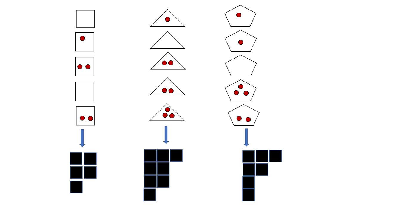
Figure 1. A configuration of $n=20$ identical balls as a multiple partition $\Lambda_{20}^{(3)}=\left(\lambda^{(1)},\lambda^{(2)},\lambda^{(3)}\right)$, where $\lambda^{(1)}=(2,2,1)$, $\lambda^{(2)}=\left(3,2,2,1\right)$, and $\lambda^{(3)}=(3,2,1,1)$.

A random multiple partition of $n$ with $k$ components is a random variable $\Lambda_{n}^{(k)}$ with values in the set $\operatorname{\mathbb{Y}}_{n}^{(k)}=\left\{\left(\lambda^{(1)},\ldots,\lambda^{(k)}\right):\;|\lambda^{(1)}|+\ldots+|\lambda^{(k)}|=n\right\}.$

Definition 2.1.

A multiple partition structure is a sequence $\mathcal{M}_{1}^{(k)}$, $\mathcal{M}_{2}^{(k)}$, $\ldots$ of distributions for $\Lambda_{1}^{(k)}$, $\Lambda_{2}^{(k)}$, $\ldots$ which is consistent in the following sense: if $n$ balls are partitioned into boxes of $k$ different types such that their configuration is $\Lambda_{n}^{(k)}$, and a ball is deleted uniformly at random (see Fig. 2), independently of $\Lambda_{n}^{(k)}$, then the multiple partition $\Lambda_{n-1}^{(k)}$ describing the configuration of the remaining balls is distributed according to $\mathcal{M}^{(k)}_{n-1}$.

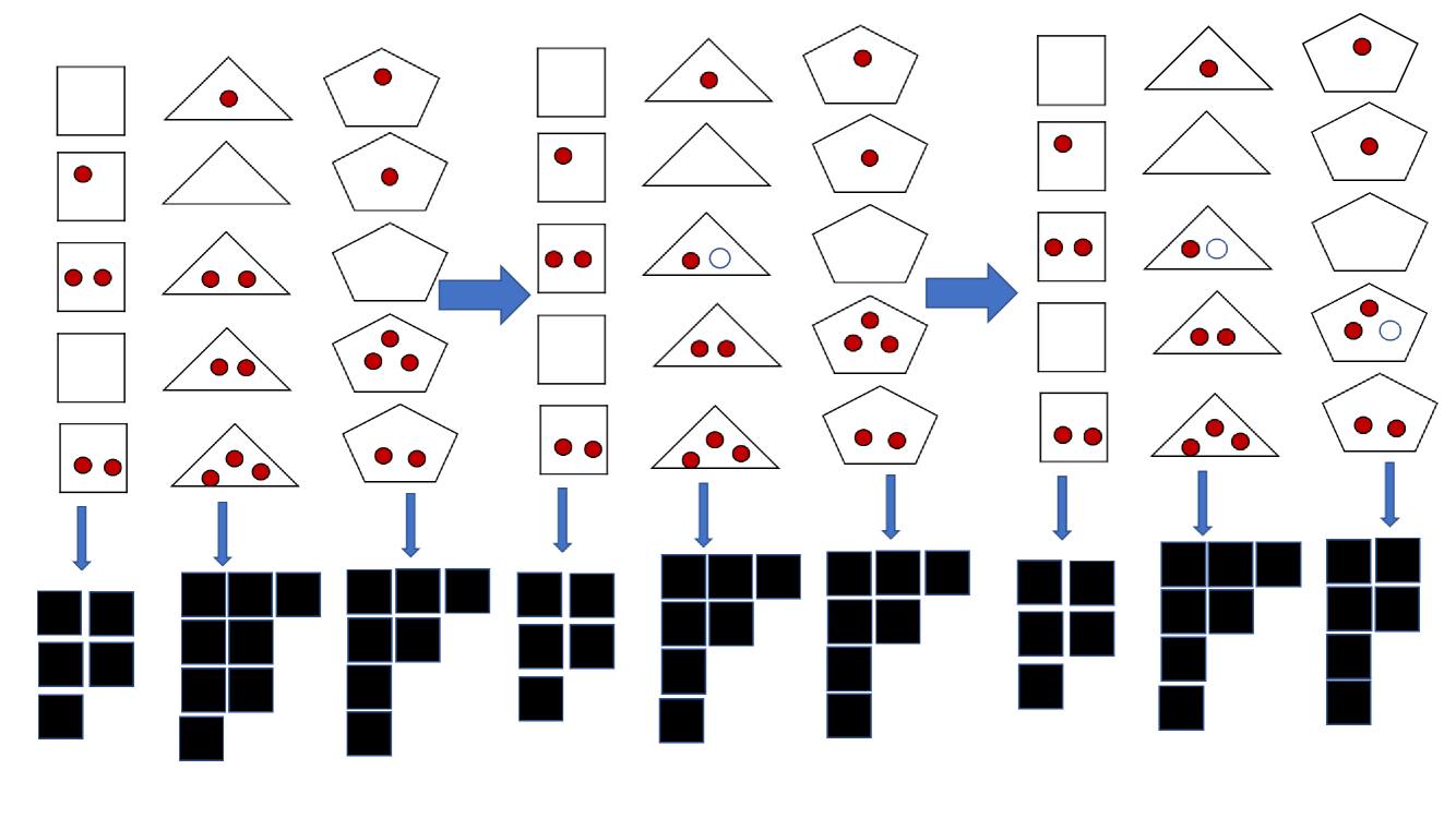
Figure 2. Each time a ball is deleted uniformly at random from a box.

If $k=1$ then a multiple partition structure is a partition structure in the sense of Kingman [18]. In the context of population genetics, Kingman considers a sample of $n$ representatives from a population, and studies the probability that there $A_{1}^{(1)}$ alleles (versions of a specific gene appeared due to mutations) represented once in the sample, $A_{2}^{(1)}$ alleles represented twice, and so on.

For an arbitrary $k$, a model of population genetics leading to investigation of multiple partition structures can be formulated as well. A gamete is a reproductive cell of an animal or plant. Assume that $n$ gametes in a sample from a very large population are classified according to the $k$ particular genes. Namely, the experiment is such that each individual from the sample is described by precisely one element from the set $S$,

$$S=S_{1}\cup\ldots\cup S_{k},\;\;S_{j}\cup S_{l}=\emptyset,\;\;1\leq j\neq l\leq k,$$

where $S_{1}$ is the set of all possible alleles of the first gene, $\ldots$, $S_{k}$ is the set of all possible alleles of the $k$-th gene. The model is of “infinite alleles type” so each $S_{l}$ contains an infinite number of elements. Denote by $A_{j}^{(l)}$ (where $1\leq j\leq n$ and $1\leq l\leq k$) the number of alleles of the $l$-th gene represented $j$ times in the sample. Then we have

$$\sum\limits_{l=1}^{k}\sum\limits_{j=1}^{n}jA_{j}^{(l)}=n,$$

and each set $\left\{A_{j}^{(l)}\right\}_{\underset{l=1,\ldots,k}{j=1,\ldots,n}}$ can be identified with a multiple partition $\Lambda_{n}^{(k)}$ of $n$ into $k$ components. A model for the allelic partition is then a probability distribution $\mathcal{M}_{n}^{(k)}$ over the set $\operatorname{\mathbb{Y}}_{n}^{(k)}$ of all multiple partitions $\Lambda_{n}^{(k)}$ of the integer $n$ into $k$ components. Since $n$ may be chosen at the experimenter’s convenience, the consistency condition as in Definition 2.1 should be satisfied. Therefore, the sequence of distributions $\left(\mathcal{M}_{n}\right)_{n=1}^{\infty}$ is a multiple partition structure in the sense of Definition 2.1.

The problem is to describe all such distributions. The representation theorem for multiple partition structures below solves this problem.

Theorem 2.2.

There is a bijective correspondence between multiple partition structures $\left(\mathcal{M}_{n}^{(k)}\right)_{n=1}^{\infty}$ and probability measures $P$ on the space

(2.2) $$\begin{split}\overline{\nabla}^{(k)}=&\biggl{\{}(x,\delta)\biggr{|}x=\left(x^{(1)},\ldots,x^{(k)}\right),\;\delta=\left(\delta^{(1)},\ldots,\delta^{(k)}\right);\\ &x^{(l)}=\left(x^{(l)}_{1}\geq x^{(l)}_{2}\geq\ldots\geq 0\right),\;\delta^{(l)}\geq 0,\;1\leq l\leq k,\\ &\mbox{where}\;\;\sum\limits_{i=1}^{\infty}x_{i}^{(l)}\leq\delta^{(l)},\;1\leq l\leq k,\;\mbox{and}\;\sum\limits_{l=1}^{k}\delta^{(l)}=1\biggl{\}}.\end{split}$$

The correspondence is determined by

(2.3) $$\mathcal{M}_{n}^{(k)}\left(\Lambda_{n}^{(k)}\right)=\int_{\overline{\nabla}^{(k)}}\mathbb{K}\left(\Lambda_{n}^{(k)},\omega\right)P(d\omega),\;\;\forall\Lambda_{n}^{(k)}\in\operatorname{\mathbb{Y}}_{n}^{(k)},$$

where $\mathbb{K}:\;\operatorname{\mathbb{Y}}_{n}^{(k)}\times\overline{\nabla}^{(k)}\rightarrow\operatorname{\mathbb{R}}$ is a kernel function. The kernel function $\mathbb{K}\left(\Lambda^{(k)}_{n},\omega\right)$ is given by

(2.4) $$\begin{split}&\mathbb{K}\left(\Lambda^{(k)}_{n},\omega\right)=\frac{n!}{\prod\limits_{l=1}^{k}|\lambda^{(l)}_{1}|!\ldots|\lambda^{(l)}_{n}|!}M_{\lambda^{(1)}}\left(x^{(1)},\delta^{(1)}\right)\ldots M_{\lambda^{(k)}}\left(x^{(k)},\delta^{(k)}\right),\end{split}$$

where $\Lambda_{n}^{(k)}=\left(\lambda^{(1)},\ldots,\lambda^{(k)}\right)$, and $M_{\lambda^{(l)}}\left(x^{(l)},\delta^{(l)}\right)$ are the extended monomial symmetric functions defined in terms of the usual monomial symmetric functions $m_{\lambda^{(l)}}(x_{1},x_{2},\ldots)$ as

(2.5) $$M_{\lambda^{(l)}}\left(x^{(l)},\delta^{(l)}\right)=\sum\limits_{p=0}^{\varrho_{1}^{(l)}}\;\frac{\left[\delta^{(l)}-\sum\limits_{j=1}^{\infty}x^{(l)}_{j}\right]^{p}}{p!}\;m_{\left(1^{\varrho_{1}^{(l)}-p}\;2^{\varrho_{2}^{(l)}}\ldots\right)}\left(x^{(l)}_{1},x^{(l)}_{2},\ldots\right).$$

In equation (2.5) the parameter $\varrho_{j}^{(l)}$ is equal to the number of rows of length $j$ in $\lambda^{(l)}$, i.e. $\lambda^{(l)}=\left(1^{\varrho_{1}^{(l)}}\;2^{\varrho_{2}^{(l)}}\ldots\right)$.

Theorem 2.2 is a corollary of a much more general Theorem 3.4, and of Proposition 3.3 stated in Section 3. Proofs of Theorem 2.2, of Theorem 3.4, and of Proposition 3.3 can be found in Section 7, and Section 8.

Remark 2.3.

If $k=1$ then $\delta^{(1)}=1$, and

(2.6) $$\overline{\nabla}^{(1)}=\left\{x=\left(x_{1}^{(1)}\geq x_{2}^{(1)}\geq\ldots\geq 0\right),\;\sum\limits_{i=1}^{\infty}x_{i}^{(1)}\leq 1\right\}.$$

In this case we obtain a bijective correspondence between the sequence $\left(\mathcal{M}_{n}^{(1)}\right)_{n=1}^{\infty}$ of measures on partitions satisfying the consistency condition of Definition 2.1 (with $k=1$), and probability measures $P$ on the space $\overline{\nabla}^{(1)}$. The correspondence is determined by

(2.7) $$\mathcal{M}_{n}^{(1)}\left(\lambda\right)=\int_{\overline{\nabla}^{(1)}}\mathbb{K}\left(\lambda,\omega\right)P(d\omega),\;\;\forall\lambda\in\operatorname{\mathbb{Y}}_{n},$$

where

$$\mathbb{K}\left(\lambda,\omega\right)=\sum\limits_{p=0}^{\varrho_{1}}\frac{\left[1-\sum\limits_{j=1}^{\infty}x_{j}\right]^{p}}{p!}m_{\left(1^{\varrho_{1}-p}2^{\varrho_{2}}\ldots\right)}\left(x_{1},x_{2},\ldots\right).$$

Formula (2.7) was first obtained by Kingman [19]. We refer the reader to the works by Kerov [14], Kerov [15], Okounkov, and Olshanski [16] for a different derivation of this formula, and for its relation to the theory of harmonic functions on branching graphs.

3. The branching graph $\Gamma_{\theta}\left(G\right)$. Representation of harmonic functions on $\Gamma_{\theta}\left(G\right))$

3.1. Multiple partition structures as coherent systems of measures on a branching graph

The description of multiple partition structures (Theorem 2.2) is a particular case of a more general general result obtained in this paper, see Theorem 3.4 below. Namely, we consider a certain branching graph $\Gamma_{\theta}\left(G\right)$, where $G$ is an arbitrary finite group, and $\theta\geq 0$ is a parameter called the Jack parameter. Our aim is to derive a canonical integral representation for harmonic functions on $\Gamma_{\theta}\left(G\right)$.

3.1.1. The branching graph $\Gamma_{\theta}(G)$

In order to define the branching graph $\Gamma_{\theta}\left(G\right)$ explicitly we use the algebra $\operatorname{Sym}\left(G\right)$ discussed in Macdonald [20], Appendix B, §5, which is a generalization of the algebra of symmetric functions $\operatorname{Sym}$ over the field of real numbers. Let $G$ be a finite group, $G_{*}=\left\{c_{1},\ldots,c_{k}\right\}$ be the set of conjugacy classes in $G$, and $G^{*}=\left\{\gamma^{1},\ldots,\gamma^{k}\right\}$ be the set of irreducible characters of $G$. We agree that $c_{1}$ contains the identity element of $G$. The algebra $\operatorname{Sym}(G)$ is defined by

$$\operatorname{Sym}\left(G\right)=\operatorname{\mathbb{R}}\left[p_{r_{1}}(c_{1}),\ldots,p_{r_{k}}(c_{k}):\;r_{1}\geq 1,\ldots,r_{k}\geq 1\right],$$

where $p_{r_{l}}\left(c_{l}\right)$ is $r_{l}$-th power sum in variables $x_{1c_{l}}$, $x_{2c_{l}}$, $\ldots$. Here $p_{r}\left(c_{l}\right)$ denotes the power symmetric function, i.e. the sequence

$$p_{r}\left(c_{l}\right)=\left(p_{r}\left(x_{1c_{l}};\right),p_{r}\left(x_{1c_{l}},x_{2c_{l}};\right),\ldots\right),$$

where for each $N=1,2,\ldots$, and each $l=1,\ldots,k$

$$p_{r}\left(x_{1c_{l}},\ldots,x_{Nc_{l}}\right)=\sum\limits_{i=1}^{N}x_{ic_{l}}^{r}.$$

The degree $r$ is assigned to $p_{r}\left(c_{l}\right)$, and the $\operatorname{Sym}(G)$ is the graded algebra.

There is an analogue of the Jack symmetric functions in $\operatorname{Sym}(G)$. Namely, for each multiple partition $\Lambda_{n}^{(k)}=\left(\lambda^{(1)},\ldots,\lambda^{(k)}\right)$ define

(3.1) $$\mathbb{P}_{\Lambda_{n}^{(k)}}\left(\gamma^{1},\ldots,\gamma^{k};\theta\right)=\prod\limits_{j=1}^{k}P_{\lambda^{(j)}}\left(\gamma^{j};\theta\right),\;\;\theta>0,$$

where $P_{\lambda^{(j)}}\left(\gamma^{j};\theta\right)$ is the Jack symmetric function expressed as a polynomial in variables $\left\{p_{r}\left(\gamma^{j}\right):\;r\geq 1\right\}$, where

(3.2) $$p_{r}\left(\gamma^{j}\right)=\sum\limits_{i=1}^{k}\frac{|G|}{|c_{i}|}\gamma^{j}\left(c_{i}\right)p_{r}\left(c_{i}\right).$$

Here $|G|$ denotes the number of elements in the group $G$, and $|c_{i}|$ denotes the number of elements in the conjugacy class $c_{i}$.

Proposition 3.1.

The following Pieri-type rule holds true

(3.3) $$\begin{split}&p_{1}(c_{1})\mathbb{P}_{\Lambda_{n}^{(k)}}\left(\gamma^{1},\ldots,\gamma^{k};\theta\right)=\sum\limits_{\widetilde{\Lambda}_{n+1}^{(k)}\in\operatorname{\mathbb{Y}}_{n+1}^{(k)}}\Upsilon_{\theta}\left(\Lambda_{n}^{(k)},\widetilde{\Lambda}_{n+1}^{(k)}\right)\mathbb{P}_{\widetilde{\Lambda}_{n+1}^{(k)}}\left(\gamma^{1},\ldots,\gamma^{k};\theta\right),\end{split}$$

where $\Upsilon_{\theta}:\operatorname{\mathbb{Y}}_{n}^{(k)}\times\operatorname{\mathbb{Y}}_{n+1}^{(k)}\rightarrow\operatorname{\mathbb{R}}_{\geq 0}$ is the multiplicity function which can be written explicitly.

We postpone the proof of Proposition 3.1 up to Section 6.

In order to present a formula for the multiplicity function $\Upsilon_{\theta}$ we need the following notation. Let $\Lambda_{n}^{(k)}\in\operatorname{\mathbb{Y}}_{n}^{(k)}$ and $\widetilde{\Lambda}_{n+1}^{(k)}\in\operatorname{\mathbb{Y}}_{n+1}^{(k)}$. Thus $\widetilde{\Lambda}_{n+1}^{(k)}=\left(\lambda^{(1)},\ldots,\lambda^{(k)}\right)$ and $\Lambda_{n}^{(k)}=\left(\mu^{(1)},\ldots,\mu^{(k)}\right)$ are such that $\sum\limits_{i=1}^{k}\left|\lambda^{(i)}\right|=n+1$, $\sum\limits_{i=1}^{k}\left|\mu^{(i)}\right|=n$. Assume that there exists $l\in\{1,\ldots,k\}$ such that $\mu^{(l)}\nearrow\lambda^{(l)}$ (i.e. $\lambda^{(l)}$ is obtained from $\mu^{(l)}$ by adding one box), and such that $\mu^{(i)}=\lambda^{(i)}$ for each $i$, $i\in\left\{1,\ldots,k\right\}$, $i\neq l$. Then we write $\Lambda_{n}^{(k)}\nearrow\widetilde{\Lambda}_{n+1}^{(k)}$.

The multiplicity function $\Upsilon_{\theta}\left(\Lambda_{n}^{(k)},\widetilde{\Lambda}_{n+1}^{(k)}\right)$ is given by

(3.4) $$\Upsilon_{\theta}\left(\Lambda_{n}^{(k)},\widetilde{\Lambda}_{n+1}^{(k)}\right)=\left\{\begin{array}[]{ll}d_{1}\chi_{\theta}\left(\mu^{(1)},\lambda^{(1)}\right),&\mu^{(1)}\nearrow\lambda^{(1)},\\ d_{2}\chi_{\theta}\left(\mu^{(2)},\lambda^{(2)}\right),&\mu^{(2)}\nearrow\lambda^{(2)},\\ \vdots&\\ d_{k}\chi_{\theta}\left(\mu^{(k)},\lambda^{(k)}\right),&\mu^{(k)}\nearrow\lambda^{(k)}\end{array}\right.$$

provided that $\Lambda_{n}^{(k)}\nearrow\widetilde{\Lambda}_{n+1}^{(k)}$, and by $\Upsilon_{\theta}\left(\Lambda_{n}^{(k)},\widetilde{\Lambda}_{n+1}^{(k)}\right)=0$ otherwise. Here $n=0,1,2,\ldots$, and we agree that $\Lambda_{0}^{(k)}=\left(\emptyset,\ldots,\emptyset\right)$. In equation (3.4) $d_{j}$ is the dimension of the irreducible representation of $G$ whose character is $\gamma^{j}$, and $\chi_{\theta}$ is the Jack edge multiplicity function given by an explicit formula

(3.5) $$\chi_{\theta}\left(\mu,\lambda\right)=\prod\limits_{\Box}\frac{\left(a(\Box)+(l(\Box)+2)\theta\right)\left(a(\Box)+1+l(\Box)\theta\right)}{\left(a(\Box)+1+(l(\Box)+1)\theta\right)\left(a(\Box)+\left(l(\Box)+1\right)\theta\right)}.$$

Here $\Box$ runs over all boxes in the $j$-th column of the diagram $\mu$, provided that the new box $\lambda\setminus\mu$ belongs to the $j$-th column of $\lambda$. If $\Box=(i,j)$ in the diagram $\mu$, then $a(\Box)=\mu_{i}-j$, and $l(\Box)=\mu^{\prime}_{j}-i$, see Macdonald [20], Chapter VI, (10.10) and (6.24.iv). It is known (see Kerov, Okounkov, and Olshanski [16], Lemma 5.1) that the coefficients $\chi_{\theta}(\mu,\lambda)$ are all positive if and only if $\theta\geq 0$. Therefore, the coefficients are $\Upsilon_{\theta}\left(\Lambda_{n}^{(k)},\widetilde{\Lambda}_{n+1}^{(k)}\right)$ are also positive for $\theta\geq 0$.

It is important that in the limit $\theta\rightarrow 0$ the Jack symmetric functions degenerate to the monomial symmetric functions, so equations (3.1) and (3.3) make sense for $\theta=0$ as well.

Let $\operatorname{\mathbb{Y}}^{(k)}$ denote the union of the sets $\operatorname{\mathbb{Y}}_{n}^{(k)}$ (with the understanding that $\operatorname{\mathbb{Y}}_{0}^{(k)}$ contains the element $\Lambda^{(k)}_{0}=\left(\emptyset,\ldots,\emptyset\right)$ only). We define a branching graph $\Gamma_{\theta}\left(G\right)$ with vertex set $\operatorname{\mathbb{Y}}^{(k)}$ by declaring that a pair of vertices $\left(\Lambda_{n-1}^{(k)},\widetilde{\Lambda}_{n}^{(k)}\right)$ (where $\Lambda_{n-1}^{(k)}\in\operatorname{\mathbb{Y}}_{n-1}^{(k)}$ and $\widetilde{\Lambda}_{n}^{(k)}\in\operatorname{\mathbb{Y}}_{n}^{(k)}$) is connected by an edge of multiplicity $\Upsilon_{\theta}\left(\Lambda_{n-1}^{(k)},\widetilde{\Lambda}_{n}^{(k)}\right)$ provided that $\Upsilon_{\theta}\left(\Lambda_{n-1}^{(k)},\widetilde{\Lambda}_{n}^{(k)}\right)\neq 0$.

For example, assume that $G=S(3)$. This group has three nonequivalent irreducible representations with dimensions $d_{1}=1$, $d_{2}=1$, and $d_{3}=2$. The very beginning of the graph $\Gamma_{\theta}\left(S(3)\right)$ is shown on Fig. 3.

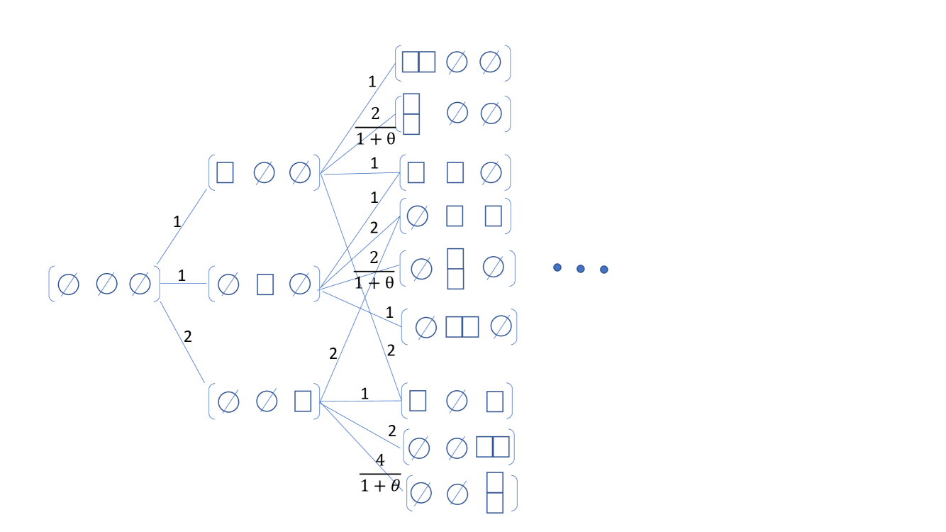
Figure 3. The branching graph $\Gamma_{\theta}\left(S(3)\right)$

3.1.2. The dimension function

Assume that $m\leq n$. The dimension function $\operatorname{DIM}_{\theta}\left(\Lambda^{(k)}_{m},\widetilde{\Lambda}^{(k)}_{n}\right)$ associated with the branch graph $\Gamma_{\theta}\left(G\right)$ is defined recurrently by the formula

(3.6) $$\operatorname{DIM}_{\theta}\left(\Lambda^{(k)}_{m},\widetilde{\Lambda}^{(k)}_{n}\right)=\sum\limits_{\Theta^{(k)}_{n-1}:\;\Theta^{(k)}_{n-1}\nearrow\widetilde{\Lambda}^{(k)}_{n}}\operatorname{DIM}_{\theta}\left(\Lambda^{(k)}_{m},\Theta^{(k)}_{n-1}\right)\Upsilon_{\theta}\left(\Theta^{(k)}_{n-1},\widetilde{\Lambda}^{(k)}_{n}\right),$$

by $\operatorname{DIM}_{\theta}\left(\Lambda^{(k)}_{m},\Lambda^{(k)}_{m}\right)=1$, and by $\operatorname{DIM}_{\theta}\left(\Lambda^{(k)}_{m},\widetilde{\Lambda}^{(k)}_{n}\right)=0$ if there is no oriented path from $\Lambda^{(k)}_{m}$ to $\widetilde{\Lambda}^{(k)}_{n}$ on $\Gamma_{\theta}\left(G\right)$. We write $\operatorname{DIM}_{\theta}\left(\Lambda^{(k)}_{m}\right)=\operatorname{DIM}_{\theta}\left(\emptyset,\Lambda^{(k)}_{m}\right).$

3.1.3. Harmonic functions. Multiple partition structures as coherent systems of measures on $\Gamma_{\theta=0}\left(G\right)$

Definition 3.2.

A function $\varphi:\;\Gamma_{\theta}\left(G\right)\rightarrow\operatorname{\mathbb{R}}_{\geq 0}$ is called harmonic on $\Gamma_{\theta}(G)$ if for each $n=1,2,\ldots$

(3.7) $$\varphi\left(\Lambda_{n-1}^{(k)}\right)=\sum\limits_{\widetilde{\Lambda}_{n}^{(k)}\in\operatorname{\mathbb{Y}}_{n}^{(k)}}\Upsilon_{\theta}\left(\Lambda_{n-1}^{(k)},\widetilde{\Lambda}_{n}^{(k)}\right)\varphi\left(\widetilde{\Lambda}_{n}^{(k)}\right),\;\;\forall\Lambda_{n-1}^{(k)}\in\operatorname{\mathbb{Y}}^{(k)}_{n-1},$$

and $\varphi\left(\Lambda^{(k)}_{0}\right)=1$. Here $\Upsilon_{\theta}$ is the multiplicity function defined by equation (3.4).

Let $\varphi$ be the harmonic function on $\Gamma_{\theta}\left(G\right)$. Set

(3.8) $$\mathcal{M}_{n}^{(k)}\left(\Lambda_{n}^{(k)}\right)=\operatorname{DIM}_{\theta}\left(\Lambda_{n}^{(k)}\right)\varphi\left(\Lambda_{n}^{(k)}\right).$$

It can be checked that each $\mathcal{M}_{n}^{(k)}$ defined by equation (3.8) is a probability measure on $\operatorname{\mathbb{Y}}_{n}^{(k)}$. The sequence $\left(\mathcal{M}_{n}^{(k)}\right)_{n=1}^{\infty}$ (where each element is defined by equation (3.8)) is called a coherent system of probability measures associated with the harmonic function $\varphi$ on $\Gamma_{\theta}\left(G\right)$.

As $\theta=0$, a relation with the multiple partition structures introduced in Section 2 arises.

Proposition 3.3.

Assume that $\theta=0$, and let $\varphi$ be a harmonic function on $\Gamma_{\theta=0}(G)$. Then the coherent sequence of probability measures $\left(\mathcal{M}_{n}^{(k)}\right)_{n=1}^{\infty}$ associated with $\varphi$ is a multiple partition structure in the sense of Definition 2.1. Conversely, each multiple partition structure $\left(\mathcal{M}_{n}^{(k)}\right)_{n=1}^{\infty}$ is a coherent system of probability measures associated with a certain harmonic function $\varphi$ on $\Gamma_{\theta=0}(G)$ via equation (3.8).

Proposition 3.3 implies that there is a one-to-one correspondence between multiple partition structures and harmonic functions on $\Gamma_{\theta=0}(G)$. This bijective relation is a generalization of the known relation (see, for example, Kerov, Okounkov, and Olshanski [16], Section 4) between the Kingman partition structures and the harmonic functions on the Young graph with the Jack edge multiplicities at $\theta=0$ (also known as the Kingman branching graph). Proof of Proposition 3.3 can be found in Section 8.

3.2. Representation of harmonic functions

In this Section we state the main result of the present paper: description of all non-negative harmonic functions $\varphi$, $\varphi:\;\Gamma_{\theta}(G)\rightarrow\operatorname{\mathbb{R}}_{\geq 0}$ defined on the set of vertices in $\Gamma_{\theta}(G)$ and normalized by the condition $\varphi\left(\Lambda_{0}^{(k)}\right)=1$, see Definition 3.2. We will show that there is a one-to-one correspondence between such functions and probability measures on the set $\Omega(G)$ defined by

(3.9) $$\begin{split}&\Omega(G)=\biggl{\{}(\alpha,\beta,\delta)\biggr{|}\alpha=\left(\alpha^{(1)},\ldots,\alpha^{(k)}\right),\beta=\left(\beta^{(1)},\ldots,\beta^{(k)}\right),\delta=\left(\delta^{(1)},\ldots,\delta^{(k)}\right);\\ &\alpha^{(l)}=\left(\alpha_{1}^{(l)}\geq\alpha_{2}^{(l)}\geq\ldots\geq 0\right),\beta^{(l)}=\left(\beta_{1}^{(l)}\geq\beta_{2}^{(l)}\geq\ldots\geq 0\right),\\ &\delta^{(1)}\geq 0,\ldots,\delta^{(k)}\geq 0,\\ &\mbox{where}\;\;\sum\limits_{i=1}^{\infty}\alpha_{i}^{(l)}+\beta_{i}^{(l)}\leq\delta^{(l)},\;1\leq l\leq k,\;\mbox{and}\;\sum\limits_{l=1}^{k}\delta^{(l)}=1\biggl{\}}.\end{split}$$

If $G$ is the group of one element, then $k=1$, and the set $\Omega(G)$ turns into the Thoma simplex. For this reason we will refer to $\Omega(G)$ as generalized Thoma set. The set $\Omega\left(G\right)$ was introduced in the work by Hora and Hirai [12] to describe general characters of the wreath products of a finite group with the infinite symmetric group.

In order to present our result we use the $\theta$-extended power sum symmetric functions $p_{r,l}^{o}\left(.;\theta\right)$. These are real-valued functions on $\Omega(G)$ defined by

(3.10) $$p_{r,l}^{o}(\alpha,\beta,\delta;\theta)=\left\{\begin{array}[]{ll}\sum\limits_{i=1}^{\infty}\left(\alpha^{(l)}_{i}\right)^{r}+(-\theta)^{r-1}\sum\limits_{i=1}^{\infty}\left(\beta_{i}^{(l)}\right)^{r},&r=2,3,\ldots,\\ \delta^{(l)},&r=1,\end{array}\right.$$

where $1\leq l\leq k$. In addition, we introduce the $\theta$-extended Jack symmetric polynomials. Namely, let $\Lambda_{n}^{(k)}=\left(\lambda^{(1)},\ldots,\lambda^{(k)}\right)\in\operatorname{\mathbb{Y}}_{n}^{(k)}$ be a multiple partition. For each $l$, $1\leq l\leq k$, the $\theta$-extended Jack symmetric polynomial $P_{\lambda^{(l)}}^{o}\left(.;\theta\right)$ is defined as follows. Consider the Jack symmetric polynomial $P_{\lambda^{(l)}}$ with the Jack parameter $\theta$, and express it in terms of the power sums $p_{r}$, $r\geq 1$. Replace each $p_{r}$ by the $\theta$-extended power symmetric functions $p_{r,l}^{o}\left(.;\theta\right)$ defined by equation (3.10). The result is a function $P_{\lambda^{(l)}}^{o}\left(.;\theta\right):\Omega(G)\rightarrow\operatorname{\mathbb{R}}$ which will be called the $\theta$-extended Jack symmetric polynomial in this paper.

Now we are ready to state the main result of the present work.

Theorem 3.4.

There is a bijective correspondence between the set of harmonic functions $\varphi$ on $\Gamma_{\theta}(G)$, and the set of probability measures $P$ on the generalized Thoma set $\Omega(G)$. This correspondence is determined by

(3.11) $$\varphi\left(\Lambda_{n}^{(k)}\right)=\int\limits_{\Omega(G)}\mathbb{K}_{\theta}\left(\Lambda_{n}^{(k)},\omega\right)P(d\omega),\;\;\forall\Lambda_{n}^{(k)}=\left(\lambda^{(1)},\ldots,\lambda^{(k)}\right)\in\operatorname{\mathbb{Y}}_{n}^{(k)},$$

where $n=1,2,...$, and $k$ is the number of conjugacy classes in $G$. The kernel $\mathbb{K}_{\theta}\left(\Lambda_{n}^{(k)},\omega\right)$ is given by

(3.12) $$\mathbb{K}_{\theta}\left(\Lambda_{n}^{(k)},\omega\right)=\prod\limits_{l=1}^{k}\frac{1}{d_{l}^{|\lambda^{(l)}|}}P_{\lambda^{(l)}}^{o}\left(\alpha,\beta,\delta;\theta\right).$$

Here $P_{\lambda^{(l)}}^{o}\left(\alpha,\beta,\delta;\theta\right)$ denotes the $\theta$-extended Jack symmetric polynomial parameterized by $\lambda^{(l)}$, and $d_{l}$ are the dimensions of irreducible representations of $G$.

The proof of Theorem 3.4 is given in Section 7.

3.3. Remarks on Theorem 3.4 and related works

3.3.1. Potential theory on the branching graph $\Gamma_{\theta}(G)$

Harmonic functions on $\Gamma_{\theta}(G)$ can be described in terms of potential theory. Namely, consider an analogue $\triangle$ of the Laplace operator on $\Gamma_{\theta}(G)$ defined by its action on a function on $\Gamma_{\theta}(G)$ as

(3.13) $$\left(\triangle f\right)\left(\Lambda_{n}^{(k)}\right)=-f\left(\Lambda_{n}^{(k)}\right)+\sum\limits_{\widetilde{\Lambda}_{n+1}^{(k)}\in\operatorname{\mathbb{Y}}_{n+1}^{(k)}}\Upsilon_{\theta}\left(\Lambda_{n}^{(k)},\widetilde{\Lambda}_{n+1}^{(k)}\right)f\left(\widetilde{\Lambda}_{n+1}^{(k)}\right).$$

Then each harmonic function $\varphi$ on $\Gamma_{\theta}(G)$ satisfies the Laplace equation

$$\left(\triangle\varphi\right)\left(\Lambda_{n}^{(k)}\right)=0.$$

Representation (3.11) is an analogue of the Poisson integral representation of nonnegative harmonic functions on the disk, see, for example, Garnett [7], Chapter 1, Theorem 3.5. Moreover, the dimension function of $\Gamma_{\theta}(G)$ defined in Section 3.1.2 can be understood as the Green function of the operator $\triangle$. Indeed, set

$$G\left(\Lambda_{m}^{(k)},\widetilde{\Lambda}_{n}^{(k)}\right)=\operatorname{DIM}_{\theta}\left(\Lambda_{m}^{(k)},\widetilde{\Lambda}_{n}^{(k)}\right),\;\;m\leq n.$$

If

$$f_{\widetilde{\Lambda}_{n}^{(k)}}\left(\Lambda_{m}^{(k)}\right)=G\left(\Lambda_{m}^{(k)},\widetilde{\Lambda}_{n}^{(k)}\right),$$

then it can be verified that

$$-\left(\triangle f_{\widetilde{\Lambda}_{n}^{(k)}}\right)\left(\Lambda_{m}^{(k)}\right)=\delta_{\widetilde{\Lambda}_{n}^{(k)},\Lambda_{m}^{(k)}},\;\;\forall\Lambda_{m}^{(k)}\in\operatorname{\mathbb{Y}}_{m}^{(k)}.$$

3.3.2. The case $\theta=0$, $k=1$

The result in this case is equivalent to the Kingman representation theorem for partition structures, see Kingman [19]. The graph $\Gamma_{\theta}(G)$ is the Kingman graph in this case.

3.3.3. The case $\theta=1$, $k=1$

If $\theta=1$ and $k=1$ (i.e. there is only one conjugacy class in $G$) then Theorem 3.4 gives a representation of the harmonic functions on the Young graph $\operatorname{\mathbb{Y}}$. This representation determines a bijective correspondence between coherent systems of probability measures on $\operatorname{\mathbb{Y}}$ and probability measures on the Thoma set. For different proofs of this result, and for discussion of its relation with the Thoma theorem [27] on characters of the infinite symmetric group we refer the reader to the book by Borodin and Olshanski [3], and to Vershik and Kerov [28].

3.3.4. The case of an arbitrary Jack parameter $\theta\geq 0$, and of $k=1$

The result in this case is due to Kerov, Okounkov, and Olshanski [16]. Our proof of Theorem 3.4 adopts the methods of Ref. [16] to the case of a general $k$ (i.e. to the case of an arbitrary finite group $G$).

3.3.5. The case $\theta=1$, $k$ is an arbitrary strictly positive integer

In this case Theorem 3.4 is reduced to the result first obtained by Hora and Hirai [12], see Theorem 3.1. in Ref. [12]. If $\theta=1$, then the branching graph $\Gamma_{\theta=1}(G)$ is that of the inductive system of wreath products $G\sim S(n)$, and the generalized Thoma set $\Omega(G)$ is the Martin boundary of $\Gamma_{\theta=1}(G)$. The proof in Hora and Hirai [12] relies on an explicit formula for the irreducible characters of the wreath products, see equation (1.8) in Hora and Hirai [12]. In the general case where $\theta\geq 0$, and $k$ is arbitrary, the relation with representation theory of wreath products is lost, and the present paper uses a different approach to prove Theorem 3.4.

4. A multiple partition structure related to the wreath products $G\sim S(n)$

In this Section we use probability measures on the wreath products $G\sim S(n)$ to construct an example of a multiple partition structure.

4.1. The wreath product $G\sim S(n)$

The wreath product $G\sim S(n)$ is the group whose underlying set is

$$\left\{\left(\left(g_{1},\ldots,g_{n}\right),s\right):\;g_{i}\in G,s\in S(n)\right\},$$

where $G$ is a finite group, and $S(n)$ is the symmetric group. The multiplication in $G\sim S(n)$ is defined by

$$\left(\left(g_{1},\ldots,g_{n}\right),s\right)\left(\left(h_{1},\ldots,h_{n}\right),t\right)=\left(\left(g_{1}h_{s^{-1}(1)},\ldots,g_{n}h_{s^{-1}(n)}\right),st\right).$$

When $n=1$, $G\sim S(1)$ is $G$. The order of $G\sim S(n)$ is $2^{n}n!$. The important fact is that both the conjugacy classes and the irreducible representations of $G\sim S(n)$ are parameterized by multiple partitions $\Lambda_{n}^{(k)}=\left(\lambda^{(1)},\ldots,\lambda^{(k)}\right)$, where $k$ is the number of conjugacy classes in $G$, and where $|\lambda^{(1)}|+\ldots+|\lambda^{(k)}|=n$, see Macdonald [20], Appendix B. The number of elements in the conjugacy class $K_{\Lambda_{n}^{(k)}}$ of $G\sim S(n)$ parameterized by $\Lambda_{n}^{(k)}=\left(\lambda^{(1)},\ldots,\lambda^{(k)}\right)$ is given by

(4.1) $$\left|K_{\Lambda_{n}^{(k)}}\right|=\frac{n!|G|^{n}}{\prod\limits_{l=1}^{k}\prod\limits_{j=1}^{n}j^{r_{j}\left(\lambda^{(l)}\right)}\left(r_{j}\left(\lambda^{(l)}\right)\right)!}\;\frac{1}{\prod\limits_{l=1}^{k}\zeta_{l}^{r_{1}\left(\lambda^{(l)}\right)+\ldots+r_{n}\left(\lambda^{(l)}\right)}},$$

where $r_{j}\left(\lambda^{(l)}\right)$ denotes the number of rows of length $j$ in the Young diagram $\lambda^{(l)}$ (in particular, the sum $r_{1}\left(\lambda^{(l)}\right)+\ldots+r_{n}\left(\lambda^{(l)}\right)$ is equal to the total number of rows in $\lambda^{(l)}$).

4.2. The Ewens probability measure on $G\sim S(n)$

Assume that

$$x=\left(\left(g_{1},\ldots,g_{n}\right),s\right)\in G\sim S(n).$$

A cycle $(i_{1},\ldots,i_{r})$ of $s$ is called of type $c_{l}$ if the product $g_{i_{r}}\ldots g_{i_{2}}g_{i_{1}}$ belongs the the conjugacy class $c_{l}$ of $G$, $1\leq l\leq k$.

Proposition 4.1.

Fix $t_{1}>0$, $\ldots$, $t_{k}>0$, and set

(4.2) $$P_{t_{1},\ldots,t_{k};n}^{\operatorname{Ewens}}(x)=\frac{t_{1}^{[x]_{c_{1}}}t_{2}^{[x]_{c_{2}}}\ldots t_{k}^{[x]_{c_{k}}}}{|G|^{n}\left(\frac{t_{1}}{\zeta_{c_{1}}}+\ldots+\frac{t_{k}}{\zeta_{c_{k}}}\right)_{n}},\;x=\left((g_{1},\ldots,g_{n}),s\right)\in G\sim S(n),$$

where $c_{1}$, $\ldots$, $c_{k}$ are the conjugacy classes of $G$, $[x]_{c_{l}}$ is the number of cycles of type $c_{l}$ in $s$, $\zeta_{c_{l}}=\frac{|G|}{|c_{l}|}$, and $(a)_{n}$ is the Pochhammer symbol. Each $P_{t_{1},\ldots,t_{k};n}^{\operatorname{Ewens}}$ is a probability measure on $G\sim S(n)$.

Proposition 4.1 will be proved in Section 9.

The measure $P_{t_{1},\ldots,t_{k};n}^{\operatorname{Ewens}}$ is called the Ewens probability measure on $G\sim S(n)$. If $G$ contains only the identity element, then $k=1$, and $P_{t_{1},\ldots,t_{k};n}^{\operatorname{Ewens}}$ turns into the Ewens probability measure on the symmetric group. We refer the reader to the paper by Olshanski [25] where the importance and different properties of the Ewens probability measures on the symmetric groups are explained. In particular, the consistency of the Ewens probability measures under the canonical projections $p_{n,n-1}:S(n)\rightarrow S(n-1)$ makes it possible to build an “$n=\infty$” versions of these measures on the space of virtual permutations, see Kerov, Olshanski, and Vershik [17]. In spite of the fact that the Ewens probability measures were studied by many researches, the Ewens measures $P_{t_{1},\ldots,t_{k};n}^{\operatorname{Ewens}}$ on the wreath products were not previously considered in the literature, to the best of the author knowledge.

4.3. The multiple partition structure $\left(\mathcal{M}_{t_{1},\ldots,t_{k};n}^{\operatorname{Ewens}}\right)_{n=1}^{\infty}$

To an element $x\in G\sim S(n)$ we assign a multiple partition $\Lambda_{n}^{(k)}\in\operatorname{\mathbb{Y}}_{n}^{(k)}$ describing the conjugacy class of $x$. Since $P_{t_{1},\ldots,t_{k};n}^{\operatorname{Ewens}}(x)$ is invariant under action of $G\sim S(n)$ on itself by conjugations, the projection $x\rightarrow\Lambda_{n}^{(k)}$ takes $P_{t_{1},\ldots,t_{k};n}^{\operatorname{Ewens}}$ to a probability measure $\mathcal{M}_{t_{1},\ldots,t_{k};n}^{\operatorname{Ewens}}$ on the set of multiple partitions $\operatorname{\mathbb{Y}}_{n}^{(k)}$. This measure will be called the Ewens probability measure on multiple partitions. In order to write $\mathcal{M}^{\operatorname{Ewens}}_{t_{1},\ldots,t_{k};\;n}$ explicitly set

(4.3) $$T_{1}=\frac{t_{1}}{\zeta_{c_{1}}},\ldots,T_{k}=\frac{t_{k}}{\zeta_{c_{k}}}.$$

Then $\mathcal{M}^{\operatorname{Ewens}}_{t_{1},\ldots,t_{k};\;n}\left(\Lambda_{n}^{(k)}\right)$ can be written as

(4.4) $$\mathcal{M}^{\operatorname{Ewens}}_{t_{1},\ldots,t_{k};\;n}\left(\Lambda_{n}^{(k)}\right)=\frac{\left(T_{1}\right)_{|\lambda^{(1)}|}\ldots\left(T_{k}\right)_{|\lambda^{(k)}|}}{\left(T_{1}+\ldots+T_{k}\right)_{n}}\frac{n!}{|\lambda^{(1)}|!\ldots|\lambda^{(k)}|!}M^{\operatorname{Ewens}}_{T_{1},|\lambda^{(1)}|}\left(\lambda^{(1)}\right)\ldots M^{\operatorname{Ewens}}_{T_{k},|\lambda^{(k)}|}\left(\lambda^{(k)}\right),$$

where $\Lambda_{n}^{(k)}=\left(\lambda^{(1)},\ldots,\lambda^{(k)}\right)\in\operatorname{\mathbb{Y}}_{n}^{(k)}$, and $M^{\operatorname{Ewens}}_{T_{l},|\lambda^{(l)}|}\left(\lambda^{(l)}\right)$, $1\leq l\leq k$, are defined by equation

(4.5) $$M_{t,n}^{\operatorname{Ewens}}(\lambda)=\frac{n!}{1^{r_{1}(\lambda)}r_{1}(\lambda)!2^{r_{2}(\lambda)}r_{2}(\lambda)!\ldots n^{r_{n}(\lambda)}r_{n}(\lambda)!}\;\frac{t^{l(\lambda)}}{(t)_{n}}.$$

Here $\lambda=\left(1^{r_{1}(\lambda)}2^{r_{2}(\lambda)}\ldots n^{r_{n}(\lambda)}\right)\in\operatorname{\mathbb{Y}}_{n}$. It is well-known that $\left(M_{t,n}^{\operatorname{Ewens}}(\lambda)\right)_{n=1}^{\infty}$ is a partition structure in the sense of Kingman [18]. Moreover, the measure $M_{t,n}^{\operatorname{Ewens}}$ has an important interpretation in the models of population genetics for the genetic variation of a sample of gametes from a large population, see Kingman [19] and the references therein. Namely, assume that a sample of $n$ gametes is taken from a population, and it is classified according to one particular gene. Denote by $P_{n}\left(r_{1},r_{2},\ldots,r_{n}\right)$ the probability that there are $r_{1}$ alleles represented once in the sample, $r_{2}$ represented twice in the sample, and so on. It was shown in the works by Ewens [6], Karlin and McGregor [13] that under suitable conditions this probability is given by

(4.6) $$P_{n}\left(r_{1},r_{2},\ldots,r_{n}\right)=M_{t,n}^{\operatorname{Ewens}}(\lambda),\;\;\lambda=\left(1^{r_{1}}2^{r_{2}}\ldots n^{r_{n}}\right).$$

Equation (4.6) is known as the Ewens sampling formula. We refer the reader to the paper by Tavar$\acute{\mbox{e}}$ [26] and to the book by Arratia, Barbour, and Tavar$\acute{\mbox{e}}$ [1] where numerous applications of the Ewens sampling formula are described. As $k=1$ the measure $\mathcal{M}^{\operatorname{Ewens}}_{t_{1},\ldots,t_{k};\;n}$ defined by equation (4.4) turns into $M_{t_{1},n}^{\operatorname{Ewens}}$. The author of the present paper expects that the methods from works by Ewens [6], Karlin and McGregor [13] can be applied to show that the distribution $\mathcal{M}^{\operatorname{Ewens}}_{t_{1},\ldots,t_{k};\;n}$ defines a realistic model for the allelic partition in the situation where $n$ gametes in a sample from a very large population are classified according to the $k$ particular genes, see discussion in Section 2. As it was explained in Section 2, a necessary condition for a measure $\mathcal{M}_{n}^{(k)}$ to define a model for the allelic partition is that the sequence of distributions $\left(\mathcal{M}_{n}\right)_{n=1}^{\infty}$ is a multiple partition structure in the sense of Definition 2.1. Here we show that this is indeed the case for the sequence $\left(\mathcal{M}_{t_{1},\ldots,t_{k};n}^{\operatorname{Ewens}}\right)_{n=1}^{\infty}$.

Proposition 4.2.

The sequence $\left(\mathcal{M}_{t_{1},\ldots,t_{k};n}^{\operatorname{Ewens}}\right)_{n=1}^{\infty}$ is a multiple partition structure.

For a proof of Proposition 4.2 we refer the reader to Section 10.

The representation theorem for multiple partition structures (see Theorem 2.2 above) gives

(4.7) $$\mathcal{M}_{t_{1},\ldots,t_{k};n}^{\operatorname{Ewens}}\left(\Lambda_{n}^{(k)}\right)=\int_{\overline{\nabla}^{(k)}}\mathbb{K}\left(\Lambda_{n}^{(k)},\omega\right)P^{\operatorname{Ewens}}_{t_{1},\ldots,t_{k}}(d\omega),$$

where $P^{\operatorname{Ewens}}_{t_{1},\ldots,t_{k}}$ is a probability measure on $\overline{\nabla}^{(k)}$. As $k=1$, the probability measure $P^{\operatorname{Ewens}}_{t_{1}}$ on $\overline{\nabla}^{(k=1)}$ assigned by formula (4.7) to $M_{t_{1},n}^{\operatorname{Ewens}}$ is known as the Poisson-Dirichlet distribution $PD(t_{1})$, see Kingman [18]. For a comprehensive account of the theory of the Poisson-Dirichlet distribution we refer the reader to the book by Feng [9], and to the references therein. Here we recall that the Poisson-Dirichlet distribution $PD(t)$ can be understood as the Poisson-Dirichlet limit of the Dirichlet distribution $D(T_{1},\ldots,T_{M})$ with density

(4.8) $$\frac{\Gamma\left(T_{1}+\ldots+T_{M}\right)}{\Gamma\left(T_{1}\right)\ldots\Gamma\left(T_{M}\right)}x_{1}^{T_{1}-1}x_{2}^{T_{2}-1}\ldots x_{M}^{T_{M}-1}$$

relative to the $(M-1)$- dimensional Lebesgue measure on the simplex

$$\triangle_{M}=\left\{(x_{1},\ldots,x_{M}):\;x_{i}\geq 0,\;x_{1}+\ldots+x_{M}=1\right\},$$

where $T_{1}$, $\ldots$, $T_{M}$ are strictly positive parameters. Assume that $(x_{1},\ldots,x_{M})$ has the Dirichlet distribution with equal parameters,

$$T_{1}=\ldots=T_{M}=\frac{t}{M-1}.$$

If $x_{(1)}\geq x_{(2)}\geq\ldots\geq x_{(M)}$ denote the $x_{j}$ arranged in descending order, then $x_{(1)}$, $x_{(2)}$, $\ldots$ converge in joint distribution as $M\rightarrow\infty$, the limit is $PD(t)$. The Poisson-Dirichlet distribution $PD(t)$ is concentrated on the set

(4.9) $$\overline{\nabla}_{0}^{(1)}=\left\{x=\left(x_{1},x_{2},\ldots,\right):\;x_{1}\geq x_{2}\geq\ldots\geq 0,\;\sum\limits_{i=1}^{\infty}x_{i}=1\right\}.$$

An interesting problem is to describe the probability measure $P^{\operatorname{Ewens}}_{t_{1},\ldots,t_{k}}$ for general $k=1,2,\ldots$. We will see that $P^{\operatorname{Ewens}}_{t_{1},\ldots,t_{k}}$ can be understood as the multiple Poisson-Dirichlet distribution.

4.4. The multiple Poisson-Dirichlet distribution. The representation theorem for $\left(\mathcal{M}_{t_{1},\ldots,t_{k};n}^{\operatorname{Ewens}}\right)_{n=1}^{\infty}$.

Let $t_{1}>0$, $\ldots$, $t_{k}>0$. For each $l$, $1\leq l\leq k$, let $x^{(l)}=\left(x^{(l)}_{1},x^{(l)}_{2},\ldots\right)$ be independent sequences of random variables such that

$$x^{(l)}\sim PD(t_{l}),\;l=1,\ldots,k.$$

Furthermore, let $\delta^{(1)}$, $\ldots$, $\delta^{(k)}$ be random variables independent of $x^{(1)}$, $\ldots$, $x^{(k)}$, and such that joint distribution of $\delta^{(1)}$, $\ldots$, $\delta^{(k)}$ is the Dirichlet distribution $D\left(t_{1},\ldots,t_{k}\right)$. The joint distribution of the sequences $\delta^{(1)}x^{(1)}$, $\ldots$, $\delta^{(k)}x^{(k)}$ is called the multiple Poisson-Dirichlet distribution $PD(t_{1},\ldots,t_{k})$.
The distribution $PD(t_{1},\ldots,t_{k})$ is concentrated on

$$\begin{split}\overline{\nabla}_{0}^{(k)}=&\biggl{\{}(x,\delta)\biggr{|}x=\left(x^{(1)},\ldots,x^{(k)}\right),\delta=\left(\delta^{(1)},\ldots,\delta^{(k)}\right);\\ &x^{(l)}=\left(x^{(l)}_{1},x^{(l)}_{2},\ldots\right),x_{1}^{(l)}\geq x_{2}^{(l)}\geq\ldots\geq 0,\;1\leq l\leq k,\\ &\delta^{(1)}\geq 0,\ldots,\delta^{(k)}\geq 0,\\ &\mbox{where}\;\;\sum\limits_{i=1}^{\infty}x_{i}^{(l)}=\delta^{(l)},\;1\leq l\leq k,\;\mbox{and}\;\sum\limits_{l=1}^{k}\delta^{(l)}=1\biggl{\}}.\end{split}$$

If $k=1$, the multiple Poisson-Dirichlet distribution turns into the usual Poisson-Dirichlet distribution $PD(t_{1})$.

4.4.1. The representation theorem for $\left(\mathcal{M}_{t_{1},\ldots,t_{k};n}^{\operatorname{Ewens}}\right)_{n=1}^{\infty}$.

In Section 11 we prove the following Theorem:

Theorem 4.3.

The multiple partition structure $\left(\mathcal{M}^{\operatorname{Ewens}}_{t_{1},\ldots,t_{k};\;n}\right)_{n=1}^{\infty}$ has the representation

$$\begin{split}&\mathcal{M}^{\operatorname{Ewens}}_{t_{1},\ldots,t_{k};\;n}\left(\Lambda_{n}^{(k)}\right)=\frac{n!}{\prod\limits_{l=1}^{k}|\lambda^{(l)}_{1}|!\ldots|\lambda^{(l)}_{n}|!}\\ &\times\int\limits_{\overline{\nabla}_{0}^{(k)}}m_{\lambda^{(1)}}(x^{(1)})\ldots m_{\lambda^{(k)}}(x^{(k)})PD(T_{1},\ldots,T_{k})\left(d\omega\right),\;\;\forall\Lambda_{n}^{(k)}=\left(\lambda^{(1)},\ldots,\lambda^{(k)}\right)\in\operatorname{\mathbb{Y}}_{n}^{(k)}.\end{split}$$

Here $m_{\lambda^{(l)}}\left(x^{(l)}\right)$ are the monomial symmetric functions, $T_{1}=\frac{t_{1}}{\zeta_{c_{1}}}$, $\ldots$, $T_{k}=\frac{t_{k}}{\zeta_{c_{k}}}$, the parameters $\zeta_{c_{l}}$ are defined by $\zeta_{c_{l}}=\frac{|G|}{|c_{l}|}$, and $PD(T_{1},\ldots,T_{k})$ is the multiple Poisson-Dirichlet distribution.

Remark 4.4.

In the simplest case $k=1$ we obtain

(4.10) $$\begin{split}&\mathcal{M}^{\operatorname{Ewens}}_{t,n}\left(\lambda\right)=\frac{n!}{|\lambda_{1}|!\ldots|\lambda_{l(\lambda)}|!}\int\limits_{\overline{\nabla}_{0}^{(1)}}m_{\lambda}(x)PD(t)\left(dx\right),\end{split}$$

where

(4.11) $$\overline{\nabla}_{0}^{(1)}=\left\{x=\left(x_{1}^{(1)}\geq x_{2}^{(1)}\geq\ldots\geq 0\right),\;\sum\limits_{i=1}^{\infty}x_{i}^{(1)}=1\right\}.$$

Equation 4.10 is the Kingman representation formula for the Ewens measure $\mathcal{M}^{\operatorname{Ewens}}_{t,n}$ on the set of Young diagrams with $n$ boxes, see Kingman [18, 19].

4.4.2. Correlation functions

A point process can be associated with $PD(t_{1},\ldots,t_{k})$, and its correlation functions can be explicitly computed.

Set $I=[0,1]$, and let $\operatorname{Conf}(I)$ be the collection of all finite and countably infinite subsets of $I$. We define an embedding $\overline{\nabla}_{0}^{(1)}\rightarrow\operatorname{Conf}(I)$ by removing all possible zero coordinates, and forgetting the ordering. Thus

$$x=\left(x_{1}\geq x_{2}\geq\ldots\geq 0\right)\rightarrow C=\left\{x_{i}\neq 0\right\}.$$

In this way we convert $x\in\overline{\nabla}_{0}^{(1)}$ into a point configuration in $I=[0,1]$. The puchforward $\mathcal{P}\mathcal{D}(t)$ of the Poisson-Dirichlet distribution $PD(t)$ is a point process on the space $[0,1]$ called the Poisson-Dirichlet process.

Assume that

$$C=\left\{X_{1},X_{2},\ldots\right\}\in\operatorname{Conf}(I)$$

is a random point configuration of the Poisson-Dirichlet process. The correlation functions of this process are characterized by equation

(4.12) $$\mathbb{E}\left(\sum\limits_{i_{1},\ldots,i_{n}}f\left(X_{i_{1}},\ldots,X_{i_{n}}\right)\right)=\int\limits_{0}^{1}\ldots\int\limits_{0}^{1}f(x_{1},\ldots,x_{n})\varrho_{n}^{PD(t)}(x_{1},\ldots,x_{n})dx_{1}\ldots dx_{n},$$

where the summation is over all $n$-tuples of pairwise distinct indices, and $f$ is a bounded compactly supported function on $I^{n}$. It is known (see Watterson [30]) that

(4.13) $$\varrho_{n}^{PD(t)}(x_{1},\ldots,x_{n})=\frac{t^{n}}{x_{1}\ldots x_{n}}\left(1-\sum\limits_{j=1}^{n}x_{j}\right)^{t-1}1_{\overline{\nabla}_{n}^{(1)}}\left(x_{1},\ldots,x_{n}\right),$$

where $\overline{\nabla}_{n}^{(1)}=\left\{\left(x_{1},\ldots,x_{n}\right):\;x_{1}\geq 0,\ldots,x_{n}\geq 0,\;x_{1}+\ldots+x_{n}\leq 1\right\}.$ Furthermore, assume that each sequence of random variables

$$x^{(l)}=\left(x_{1}^{(l)}\geq x_{2}^{(l)}\geq\ldots\geq 0\right),\;\;l=1,\ldots,k,$$

forms the Poisson-Dirichlet point process on $I=[0,1]$, and the sequences $x^{(l)}$ are independent. Let $\delta^{(1)}$, $\ldots$, $\delta^{(k)}$ be random variables independent on $x^{(l)}$’s whose joint distribution is $D(T_{1},\ldots,T_{k})$. The point process formed by $\delta^{(l)}x^{(l)}=\left(\delta^{(l)}x^{(l)}_{1}\geq\delta^{(l)}x_{2}^{(l)}\geq\ldots\right)$, $l=1,\ldots,k$, is called the multiple Poisson-Dirichlet point process $\mathcal{P}\mathcal{D}(T_{1},\ldots,T_{k})$. It is not hard to see that the correlation functions $\varrho_{n_{1},\ldots,n_{k}}^{\mathcal{P}\mathcal{D}(T_{1},\ldots,T_{k})}\left(x_{1}^{(1)},\ldots,x_{n_{1}}^{(1)},\ldots,x_{1}^{(k)},\ldots,x_{n_{k}}^{(k)}\right)$ of the multiple Poisson-Dirichlet point process $\mathcal{P}\mathcal{D}(T_{1},\ldots,T_{k})$ can be expressed in terms of the correlation functions $\varrho_{n}^{PD(T)}(x_{1},\ldots,x_{n})$ of the Poisson-Dirichlet point process (these correlation functions are given explicitly by equation (4.13)). Namely, we have

(4.14) $$\begin{split}&\varrho_{n_{1},\ldots,n_{k}}^{\mathcal{P}\mathcal{D}(T_{1},\ldots,T_{k})}\left(x_{1}^{(1)},\ldots,x_{n_{1}}^{(1)},\ldots,x_{1}^{(k)},\ldots,x_{n_{k}}^{(k)}\right)\\ &=\underset{\delta_{1}+\ldots+\delta_{k}=1}{\underset{\delta_{1}\geq 0,\ldots,\delta_{k}\geq 0}{\int\ldots\int}}\varrho_{n_{1}}^{PD(T_{1})}\left(\frac{x_{1}^{(1)}}{\delta_{1}},\ldots,\frac{x_{n_{1}}^{(1)}}{\delta_{1}}\right)\ldots\varrho_{n_{k}}^{PD(T_{k})}\left(\frac{x_{1}^{(k)}}{\delta_{k}},\ldots,\frac{x_{n_{k}}^{(k)}}{\delta_{k}}\right)\\ &\times\frac{\Gamma(T_{1})\ldots\Gamma(T_{k})}{\Gamma(T_{1}+\ldots+T_{k})}\delta_{1}^{T_{1}-n_{1}-1}\delta_{k}^{T_{k}-n_{k}-1}d\delta_{1}\ldots d\delta_{k},\end{split}$$

where $n_{1}$, $\ldots$, $n_{k}$ are arbitrary strictly positive integers.

5. The algebra $\operatorname{Sym}_{\theta}^{\ast}\left(G\right)$ and the asymptotics of its elements

In this Section we introduce and study the algebra $\operatorname{Sym}_{\theta}^{\ast}\left(G\right)$. This algebra, $\operatorname{Sym}_{\theta}^{\ast}\left(G\right)$, is a generalization of the algebra of $\theta$-shifted symmetric polynomials described in Kerov, Okounkov, and Olshanski [16], Section 7. We will see that Theorem 3.4 is a consequence of certain asymptotic result for the elements of $\operatorname{Sym}_{\theta}^{\ast}\left(G\right)$ realized as real-valued functions on the set $\operatorname{\mathbb{Y}}_{n}^{(k)}$ of all multiple partitions of $n$ with $k$ components.

5.1. The algebra $\operatorname{Sym}_{\theta}^{\ast}\left(G\right)$

Recall that $G_{\ast}=\left\{c_{1},\ldots,c_{k}\right\}$ denotes the set of conjugacy classes of $G$. To each conjugacy class from $G_{\ast}$ we assign a sequence of variables

$$x_{c_{1}}=\left(x_{1c_{1}},x_{2c_{1}},\ldots\right),\ldots,x_{c_{k}}=\left(x_{1c_{k}},x_{2c_{k}},\ldots\right).$$

For each $1\leq l\leq k$, and each $N=1,2,\ldots$ set

(5.1) $$p_{r}^{\ast}\left(x_{1c_{l}},\ldots,x_{Nc_{l}};\theta\right)=\sum\limits_{i=1}^{N}\left(x_{ic_{l}}-\theta i\right)^{r}-\left(-\theta i\right)^{r}$$

where $r=1,2,\ldots$. These polynomials are used to introduce the $\theta$-shifted analogues of the power symmetric functions as sequences

$$p_{r}^{\ast}\left(c_{1};\theta\right)=\left(p_{r}^{\ast}\left(x_{1c_{1}};\theta\right),p_{r}^{\ast}\left(x_{1c_{1}},x_{2c_{1}};\theta\right),\ldots\right),\ldots,p_{r}^{\ast}\left(c_{k};\theta\right)=\left(p_{m}^{\ast}\left(x_{1c_{k}};\theta\right),p_{r}^{\ast}\left(x_{1c_{k}},x_{2c_{k}};\theta\right),\ldots\right).$$

The algebra $\operatorname{Sym}_{\theta}^{\ast}\left(G\right)$ is defined by

$$\operatorname{Sym}_{\theta}^{\ast}\left(G\right)=\operatorname{\mathbb{R}}\left[p_{r}^{\ast}\left(c_{l};\theta\right):r\geq 1;\;l=1,\ldots,k\right].$$

We assign degree $r$ to $p_{r}^{\ast}\left(c_{l};\theta\right)$, and the $\operatorname{Sym}_{\theta}^{\ast}\left(G\right)$ is a graded algebra. If $f_{\theta}^{\ast}$ is an arbitrary element of $\operatorname{Sym}_{\theta}^{\ast}\left(G\right)$, then $\deg\left(f_{\theta}^{\ast}\right)$ denotes the degree of the highest homogeneous component of $f_{\theta}^{\ast}$.

In addition to $\operatorname{Sym}_{\theta}^{\ast}\left(G\right)$ we use the algebra $\operatorname{Sym}(G)$,

$$\operatorname{Sym}\left(G\right)=\operatorname{\mathbb{R}}\left[p_{r}\left(c_{l}\right):r\geq 1;l=1,\ldots,k\right],$$

see Section 3.1.1. Here $p_{r}\left(c_{l}\right)$ denotes the power sum symmetric function associated with $p_{r}^{\ast}\left(c_{l};\theta\right)$ and defined as in Section 3.1.1.

Below we use the map

$$\left[\;\right]:\;\operatorname{Sym}_{\theta}^{\ast}\left(G\right)\rightarrow\operatorname{Sym}\left(G\right)$$

defined as follows. Assume that $f_{\theta}^{\ast}$ is an arbitrary element of $\operatorname{Sym}_{\theta}^{\ast}\left(G\right)$. Then $f_{\theta}^{\ast}$ is a linear combination of monomials in variables $p_{r}^{\ast}\left(c_{l};\theta\right)$, where $r\geq 1$ and $l=1,\ldots,k$. The function $[f^{\ast}_{\theta}]\in\operatorname{Sym}(G)$ is obtained from $f_{\theta}^{\ast}\in\operatorname{Sym}_{\theta}^{\ast}\left(G\right)$ by choosing the homogeneous component of the highest degree of $f_{\theta}^{\ast}$, and by replacing each $p_{r}^{\ast}\left(c_{l};\theta\right)$ by $p_{r}\left(c_{l}\right)$ in this homogeneous component. By definition, $\deg(f^{\ast}_{\theta})$ is the degree of $[f^{\ast}_{\theta}]$. Note that if $f_{\theta}^{\ast}\in\operatorname{Sym}_{\theta}^{\ast}\left(G\right)$ is evaluated at variables $x_{1c_{1}}$, $\ldots$, $x_{N_{1}c_{1}}$; $\ldots$; $x_{1c_{k}}$, $\ldots$, $x_{N_{k}c_{k}}$, then $[f_{\theta}^{\ast}]$ is the highest degree homogeneous component of the polynomial $f_{\theta}^{\ast}$ in variables $x_{1c_{1}}$, $\ldots$, $x_{N_{1}c_{1}}$; $\ldots$; $x_{1c_{k}}$, $\ldots$, $x_{N_{k}c_{k}}$.

For example, assume that $G=S(3)$. Then $G_{\ast}=\left\{c_{1},c_{2},c_{3}\right\}$, where

$$c_{1}=\left\{(1)(2)(3)\right\},\;\;c_{2}=\left\{(12)(3),(13)(2),(1)(23)\right\},\;\;c_{3}=\left\{(123),(132)\right\}$$

are the conjugacy classes of $S(3)$. The algebra $\operatorname{Sym}_{\theta}^{\ast}\left(S(3)\right)$ is that of polynomials in variables $\left\{p_{m}^{\ast}\left(c_{l};\theta\right):m\geq 1;\;l=1,2,3\right\}$ over $\operatorname{\mathbb{R}}$. If

$$f_{\theta}^{\ast}=2\left(p_{3}^{\ast}\left(c_{1};\theta\right)\right)^{2}p_{1}^{\ast}\left(c_{2};\theta\right)+3p_{2}^{\ast}\left(c_{3};\theta\right)p_{5}^{\ast}\left(c_{2};\theta\right)-27\left(p_{1}^{\ast}\left(c_{2};\theta\right)\right)^{2}p_{3}^{\ast}\left(c_{3};\theta\right),$$

then $f_{\theta}^{\ast}$ has two homogeneous components. The homogeneous component of the highest degree of $f_{\theta}^{\ast}$ is

$$2\left(p_{3}^{\ast}\left(c_{1};\theta\right)\right)^{2}p_{1}^{\ast}\left(c_{2};\theta\right)+3p_{2}^{\ast}\left(c_{3};\theta\right)p_{5}^{\ast}\left(c_{2};\theta\right),$$

so $\deg\left(f_{\theta}^{\ast}\right)=7$. We then obtain that

$$[f_{\theta}^{\ast}]=2\left(p_{3}\left(c_{1}\right)\right)^{2}p_{1}\left(c_{2}\right)+3p_{2}\left(c_{3}\right)p_{5}\left(c_{2}\right).$$

Below we are interested in the following realization of $\operatorname{Sym}_{\theta}^{\ast}\left(G\right)$. For each $\Lambda_{n}^{(k)}\in\operatorname{\mathbb{Y}}_{n}^{(k)}$ we define the sequences $x_{c_{1}}$, $\ldots$, $x_{c_{k}}$ as

$$x_{c_{1}}=\left(\lambda^{(1)}_{1},\ldots,\lambda_{l(\lambda^{(1)})}^{(1)},0,0,\ldots\right),\ldots,x_{c_{k}}=\left(\lambda^{(k)}_{1},\ldots,\lambda_{l(\lambda^{(k)})}^{(k)},0,0,\ldots\right).$$

Then each element of $\operatorname{Sym}_{\theta}^{\ast}\left(G\right)$ can be understood as a function $f^{\ast}_{\theta}:\operatorname{\mathbb{Y}}_{n}^{(k)}\rightarrow\operatorname{\mathbb{R}}$. We are interested in the asymptotics of $f^{\ast}_{\theta}\left(\Lambda_{n}^{(k)}\right)$ as $n\rightarrow\infty$, and $k$ remains fixed.

5.2. The generalized Thoma set $\Omega\left(G\right)$. The algebra homomorphism $\varphi_{\alpha,\beta,\delta}$

Let

$$[0,1]^{\infty}=\left\{x:x=\left(x_{1},x_{2},\ldots\right);\;\;x_{i}\in[0,1],\;\;i=1,2,\ldots\right\}$$

be the set of sequences of real numbers taking values in the closed unit interval $[0,1]$. The set $[0,1]^{\infty}$ can be regarded as the direct product of countably many copies of $[0,1]$. We equip $[0,1]^{\infty}$ with the product topology. In this topology $[0,1]^{\infty}$ is a compact set. Introduce

$$I_{k}^{\infty}=\underset{k\;\mbox{times}}{\underbrace{[0,1]^{\infty}\times\ldots\times[0,1]^{\infty}}},$$

and

$$\Delta_{k}=\left\{\delta=\left(\delta^{(1)},\ldots,\delta^{(k)}\right)\biggr{|}\delta^{(1)}\geq 0,\ldots,\delta^{(k)}\geq 0,\;\sum\limits_{l=1}^{k}\delta^{(l)}=1\right\}.$$

Let $G$ be a finite group with $k$ conjugacy classes. The generalized Thoma set $\Omega\left(G\right)$ is a subset of $I_{k}^{\infty}\times I_{k}^{\infty}\times\Delta_{k}$ defined by equation (3.9). It is not hard to verify that $\Omega(G)$ is closed in $I_{k}^{\infty}\times I_{k}^{\infty}\times\Delta_{k}$, and it itself is compact.

To each point $(\alpha,\beta,\delta)\in\Omega(G)$ we associate an algebra homomorphism

$$\varphi_{\alpha,\beta,\delta}:\;\;\operatorname{Sym}\left(G\right)\rightarrow\operatorname{\mathbb{R}}$$

defined by the formula

(5.2) $$\varphi_{\alpha,\beta,\delta}\left(p_{r}(c_{l})\right)=\left\{\begin{array}[]{ll}\sum\limits_{i=1}^{\infty}\left(\alpha^{(l)}_{i}\right)^{r}+(-\theta)^{r-1}\sum\limits_{i=1}^{\infty}\left(\beta_{i}^{(l)}\right)^{r},&r=2,3,\ldots,\\ \delta^{(l)},&r=1,\end{array}\right.$$

where $1\leq l\leq k$.

Proposition 5.1.

The functions $p_{r,l}^{o}:\;\Omega\left(G\right)\rightarrow\operatorname{\mathbb{R}}$ defined by $p_{r,l}^{o}\left(\alpha,\beta,\delta;\theta\right)=\varphi_{\alpha,\beta,\delta}\left(p_{r}\left(c_{l}\right)\right)$ are continuous. Here $1\leq l\leq k$, $r\geq 1$, and $\varphi_{\alpha,\beta,\delta}\left(p_{r}\left(c_{l}\right)\right)$ is given by equation (5.2).

Proof.

For $r=1$ the claim of Proposition 5.1 is obvious. Assume that $r\geq 2$. Let $\left(\alpha(n),\beta(n),\delta(n)\right)_{n=1}^{\infty}$ be a sequence of points in $\Omega(G)$ which converges to some point $(\alpha,\beta,\delta)$ in $\Omega(G)$. We need to show that

$$\underset{n\rightarrow\infty}{\lim}p_{r,l}^{o}\left(\alpha(n),\beta(n),\delta(n);\theta\right)=p_{r,l}^{o}\left(\alpha,\beta,\delta;\theta\right).$$

It is enough to show that $\sum\limits_{i=1}^{\infty}\left(\alpha_{i}^{(l)}\right)^{r}$ and $\sum\limits_{i=1}^{\infty}\left(\beta_{i}^{(l)}\right)^{r}$ converge uniformly in $\alpha^{(l)}$ and $\beta^{(l)}$, so we will be able to interchange the sums and the limits. Note that the condition

$$\sum\limits_{i=1}^{\infty}\left(\alpha_{i}^{(l)}+\beta_{i}^{(l)}\right)\leq\delta^{(l)}$$

implies $\alpha_{i}^{(l)}\leq\frac{\delta^{(l)}}{i}$, and $\beta_{i}^{(l)}\leq\frac{\delta^{(l)}}{i}$ for $i=1,2,\ldots$. Indeed, assume that $\alpha_{N}^{(l)}>\frac{\delta^{(l)}}{N}$ for some $N$. Since $\alpha_{1}^{(l)}\geq\ldots\geq\alpha_{N-1}^{(l)}\geq\alpha_{N}^{(l)}$, we should also have

$$\alpha_{1}^{(l)}>\frac{\delta^{(l)}}{N},\ldots,\alpha_{N-1}^{(l)}>\frac{\delta^{(l)}}{N}.$$

In addition, $\sum\limits_{i=1}^{N}\alpha_{i}^{(l)}\leq\delta^{(l)}$. Then we obtain

$$\frac{\delta^{(l)}}{N}<\alpha_{N}^{(l)}\leq\delta^{(l)}-\alpha_{1}^{(l)}-\ldots-\alpha_{N-1}^{(l)}<\frac{\delta^{(l)}}{N},$$

which is a contradiction. Thus the convergence of $\sum\limits_{i=1}^{\infty}\left(\alpha_{i}^{(l)}\right)^{r}$ and $\sum\limits_{i=1}^{\infty}\left(\beta_{i}^{(l)}\right)^{r}$ is uniform in $\alpha^{(l)}$ and $\beta^{(l)}$, and the statement of Proposition 5.1 follows. ∎

Given an arbitrary element $f\in\operatorname{Sym}(G)$, we consider a continuous function $f^{o}:\;\Omega(G)\rightarrow\operatorname{\mathbb{R}}$ defined by

(5.3) $$f^{o}\left(\alpha,\beta,\delta;\theta\right)=\varphi_{\alpha,\beta,\delta}\left(f\right),\;\;\left(\alpha,\beta,\delta\right)\in\Omega\left(G\right).$$

Namely, $f^{o}\left(\alpha,\beta,\delta;\theta\right)$ is obtained from $f$ by expressing the element $f$ of $\operatorname{Sym}(G)$ as a polynomial in variables $\left\{p_{r}(c_{l}):\;l=1,\ldots,k;r\geq 1\right\}$, and by subsequent replacing each $p_{r}(c_{l})$ by $\varphi_{\alpha,\beta,\delta}\left(p_{r}(c_{l})\right)$ defined by (5.2). Equations (5.2) and (5.3) define the algebra homomorphism between $\operatorname{Sym}(G)$ and the space $C(\Omega(G))$ of real continuous functions on $\Omega(G)$.

Proposition 5.2.

Consider the map from the algebra $\operatorname{Sym}\left(G\right)$ into the space $C\left(\Omega(G)\right)$ of real continuous functions with supremum norm defined by equations (5.2) and (5.3). The image of $\operatorname{Sym}\left(G\right)$ under this map is dense in $C\left(\Omega\left(G\right)\right)$ in the norm topology.

Proof.

According to the Stone-Weierstrass theorem it is enough to check that the subalgebra of $C\left(\Omega\left(G\right)\right)$ which is the image of $\operatorname{Sym}\left(G\right)$ does not vanish at any point of $\Omega\left(G\right)$, and separates points of $\Omega\left(G\right)$. The first fact is obvious since the image of $\operatorname{Sym}\left(G\right)$ contains a constant non-zero function. Using equation (5.2) we derive the following formula

(5.4) $$\sum\limits_{r=1}^{\infty}\frac{1}{z^{r}}p_{r,l}^{o}\left(\alpha,\beta,\delta;\theta\right)=\sum\limits_{i=1}^{\infty}\frac{\alpha_{i}^{(l)}}{z-\alpha_{i}^{(l)}}+\sum\limits_{i=1}^{\infty}\frac{\beta_{i}^{(l)}}{z+\theta\beta_{i}^{(l)}}+\frac{1}{z}\left[\delta^{(l)}-\sum\limits_{i=1}^{\infty}\alpha_{i}^{(l)}-\sum\limits_{i=1}^{\infty}\beta_{i}^{(l)}\right],$$

where $l=1,\ldots,k$. Denote by $R_{l}\left(z;\alpha,\beta,\delta;\theta\right)$ the left-hand side of the equation above. Assume that $\left(\hat{\alpha},\hat{\beta},\hat{\delta}\right)\neq\left(\check{\alpha},\check{\beta},\check{\delta}\right)$ are two distinct points of $\Omega\left(G\right)$. Then there exists $l$, $l\in\left\{1,\ldots,k\right\}$, such that

$$\left(\hat{\alpha}^{(l)},\hat{\beta}^{(l)},\hat{\delta}^{(l)}\right)\neq\left(\check{\alpha}^{(l)},\check{\beta}^{(l)},\check{\delta}^{(l)}\right).$$

For such $l$ equation (5.4) implies $R_{l}\left(z;\hat{\alpha},\hat{\beta},\hat{\delta};\theta\right)\neq R_{l}\left(z;\check{\alpha},\check{\beta},\check{\delta};\theta\right)$, and it follows that

$$p_{r,l}^{o}\left(z;\hat{\alpha},\hat{\beta},\hat{\delta};\theta\right)\neq p_{r,l}^{o}\left(z;\check{\alpha},\check{\beta},\check{\delta};\theta\right),$$

i.e. the image of $\operatorname{Sym}(G)$ in $C\left(\Omega(G)\right)$ separates points. ∎

5.3. The embedding of multiple partitions into $\Omega(G)$

Assume that

$$\Lambda_{n}^{(k)}=\left(\lambda^{(1)},\ldots,\lambda^{(k)}\right)\in\operatorname{\mathbb{Y}}_{n}^{(k)}.$$

Each $\lambda^{(l)}$, $1\leq l\leq k$, can be considered as a a collection of boxes, namely

$$\lambda^{(l)}=\left\{b_{i,j}^{(l)}:\;1\leq i\leq l\left(\lambda^{(l)}\right),\;\;1\leq j\leq\lambda_{i}^{(l)}\right\}.$$

Recall that the $\theta$-content of the box $b_{i,j}^{(l)}$ is defined by

$$c_{\theta}\left(b_{i,j}^{(l)}\right)=(j-1)-\theta(i-1).$$

A box $b_{i,j}^{(l)}\in\lambda^{(l)}$ is said to be positive if $c_{\theta}\left(b_{i,j}^{(l)}\right)>0$, and it is called negative if $c_{\theta}\left(b_{i,j}^{(l)}\right)\leq 0$. Each $\lambda^{(l)}$, $1\leq l\leq k$, can be represented as a union of disjoint subsets of its positive and negative boxes, i.e. $\lambda^{(l)}=\lambda^{(l)}_{+}\cup\lambda^{(l)}_{-}$, where

$$\lambda_{+}^{(l)}=\left\{b_{i,j}^{(l)}\in\lambda^{(l)}\biggr{|}c_{\theta}\left(b_{i,j}^{(l)}\right)>0\right\},\;\;\;\lambda_{-}^{(l)}=\left\{b_{i,j}^{(l)}\in\lambda^{(l)}\biggr{|}c_{\theta}\left(b_{i,j}^{(l)}\right)\leq 0\right\}.$$

Denote by $r^{(l)}$ the number of rows in $\lambda_{+}^{(l)}$, and by $a_{1}^{(l)}$, $a_{2}^{(l)}$, $\ldots$, $a_{r^{(l)}}^{(l)}$ the lengths of the first, of the second, $\ldots$, of the $r^{(l)}$th row of $\lambda_{+}^{(l)}$. In addition, denote by $s^{(l)}$ the number of columns in $\lambda^{(l)}_{-}$, and by $b_{1}^{(l)}$, $b_{2}^{(l)}$,…,$b_{s^{(l)}}^{(l)}$ the lengths of the first, of the second, and of the $s^{(l)}$th column of $\lambda_{-}^{(l)}$. For each $1\leq l\leq k$ we have

$$a_{1}^{(l)}\geq\ldots\geq a_{r^{(l)}}^{(l)}>0,\;\;b_{1}^{(l)}\geq\ldots\geq b_{s^{(l)}}^{(l)}>0.$$

Also, the following condition is satisfied

(5.5) $$\sum\limits_{i=1}^{r^{(l)}}a_{i}^{(l)}+\sum\limits_{i=1}^{s^{(l)}}b_{i}^{(l)}=\left|\lambda^{(l)}\right|,\;\;\;\sum\limits_{l=1}^{k}\left|\lambda^{(l)}\right|=n.$$

Set

(5.6) $$\frac{1}{n}W_{\Lambda_{n}^{(k)}}=\left(\alpha\left(\Lambda_{n}^{(k)},n\right),\beta\left(\Lambda_{n}^{(k)},n\right),\delta\left(\Lambda_{n}^{(k)},n\right)\right),$$

where

(5.7) $$\begin{split}&\alpha\left(\Lambda_{n}^{(k)},n\right)=\left(\alpha^{(1)}\left(\lambda^{(1)},n\right),\ldots,\alpha^{(k)}\left(\lambda^{(k)},n\right)\right),\\ &\beta\left(\Lambda_{n}^{(k)},n\right)=\left(\beta^{(1)}\left(\lambda^{(1)},n\right),\ldots,\beta^{(k)}\left(\lambda^{(k)},n\right)\right),\\ &\delta\left(\Lambda_{n}^{(k)},n\right)=\left(\delta^{(1)}\left(\lambda^{(1)},n\right),\ldots,\delta^{(k)}\left(\lambda^{(k)},n\right)\right).\end{split}$$

The entries $\alpha^{(l)}\left(\lambda^{(l)},n\right)$, $\beta^{(l)}\left(\lambda^{(l)},n\right)$, and $\delta^{(l)}\left(\lambda^{(l)},n\right)$ are defined by

(5.8) $$\alpha^{(l)}\left(\lambda^{(l)},n\right)=\left(\frac{a_{1}^{(l)}}{n},\ldots,\frac{a_{r^{(l)}}^{(l)}}{n},0,0,\ldots\right),$$

(5.9) $$\beta^{(l)}\left(\lambda^{(l)},n\right)=\left(\frac{b_{1}^{(l)}}{n},\ldots,\frac{b_{s^{(l)}}^{(l)}}{n},0,0,\ldots\right),$$

and

(5.10) $$\delta^{(l)}\left(\lambda^{(l)},n\right)=\frac{1}{n}\left|\lambda^{(l)}\right|,$$

where $1\leq l\leq k$. Equation (5.5) implies

$$\sum\limits_{i=1}^{\infty}\left(\alpha_{i}^{(l)}\left(\lambda^{(l)},n\right)+\beta_{i}^{(l)}\left(\lambda^{(l)},n\right)\right)=\delta^{(l)}\left(\lambda^{(l)},n\right).$$

We see that $\frac{1}{n}W_{\Lambda_{n}^{(k)}}$ defined by equation (5.6) is an element of $\Omega(G)$. Moreover, it is not hard to see that each point of $\Omega\left(G\right)$ can be approximated by points $\frac{1}{n}W_{\Lambda_{n}^{(k)}}$ with $\Lambda_{n}^{(k)}\in\operatorname{\mathbb{Y}}_{n}^{(k)}$.

5.4. Asymptotics of $f^{\ast}_{\theta}\left(\Lambda_{n}^{(k)}\right)$ as $n\rightarrow\infty$

Here we prove the following Theorem

Theorem 5.3.

To each $\Lambda_{n}^{(k)}=\left(\lambda^{(1)},\ldots,\lambda^{(k)}\right)\in\operatorname{\mathbb{Y}}_{n}^{(k)}$ associate the decreasing sequences $x_{c_{1}}$, $\ldots$, $x_{c_{k}}$ of positive real numbers according to the formulae

$$x_{c_{1}}=\left(\lambda^{(1)}_{1},\ldots,\lambda_{l(\lambda^{(1)})}^{(1)},0,0,\ldots\right),\ldots,x_{c_{k}}=\left(\lambda^{(k)}_{1},\ldots,\lambda_{l(\lambda^{(k)})}^{(k)},0,0,\ldots\right).$$

Then each element of $\operatorname{Sym}^{\ast}_{\theta}\left(G\right)$ gives rise a function $f^{\ast}_{\theta}:\operatorname{\mathbb{Y}}_{n}^{(k)}\rightarrow\operatorname{\mathbb{R}}$. Set $f=\left[f_{\theta}^{\ast}\right]$, where $[.]$ denotes the map from $\operatorname{Sym}_{\theta}^{\ast}\left(G\right)$ into $\operatorname{Sym}\left(G\right)$ defined in Section 5.1. Let $f^{o}$ be the image of $f$ under the algebra homorphism of $\operatorname{Sym}(G)$ into $C\left(\Omega(G)\right)$ defined by equations (5.2), (5.3). Then for each $\Lambda_{n}^{(k)}\in\operatorname{\mathbb{Y}}_{n}^{(k)}$ we can write

(5.11) $$\frac{1}{n^{\deg\left({f^{\ast}_{\theta}}\right)}}f^{\ast}_{\theta}\left(\Lambda_{n}^{(k)}\right)=f^{0}\left(\alpha\left(\Lambda_{n}^{(k)},n\right),\beta\left(\Lambda_{n}^{(k)},n\right),\delta\left(\Lambda_{n}^{(k)},n\right);\theta\right)+O\left(\frac{1}{\sqrt{n}}\right),$$

as $n\rightarrow\infty$, where the $O\left(\frac{1}{\sqrt{n}}\right)$ bound for the remainder depends only on $f^{\ast}_{\theta}$ and it is uniform in $\Lambda_{n}^{(k)}$. Here $\alpha\left(\Lambda_{n}^{(k)},n\right)$, $\beta\left(\Lambda_{n}^{(k)},n\right)$, $\delta\left(\Lambda_{n}^{(k)},n\right)$ are defined by equations (5.7)-(5.10).

Remark 5.4.

(a) For $k=1$ and arbitrary $\theta\geq 0$ the result is obtained in Kerov, Okounkov, and Olshanski [16], Theorem 7.1. We use Theorem 7.1 of Ref. [16] in the proof of our Theorem 5.3 below.
(b) A pedagogical account of the proof of the simplest case (where $k=1$, $\theta=1$) can be found in Borodin and Olshanski [3], Chapter 6, where the relation with the Thoma theorem for the infinite symmetric group is explained.

Proof.

Assume that $f_{\theta}^{\ast}=p_{r}^{\ast}\left(c_{l};\theta\right)$ for some $l\in\left\{1,\ldots,k\right\}$. Then

(5.12) $$f_{\theta}^{\ast}\left(\Lambda_{n}^{(k)}\right)=p_{r}^{\ast}\left(\lambda^{(l)}_{1},\ldots,\lambda^{(l)}_{l\left(\lambda^{(l)}\right)};\theta\right),$$

where the right-hand side of equation (5.12) is defined by equation (5.1), and $\deg(f_{\theta}^{\ast})=r$. Theorem 7.1 in Kerov, Okounkov, and Olshanski [16] gives

(5.13) $$\left|p_{r}^{\ast}\left(\lambda^{(l)}_{1},\ldots,\lambda^{(m)}_{l\left(\lambda^{(l)}\right)};\theta\right)-\sum\limits_{j=1}^{r^{(l)}}\left(a_{j}^{(l)}\right)^{r}-(-\theta)^{r-1}\sum\limits_{j=1}^{s^{(l)}}\left(b_{j}^{(l)}\right)^{r}\right|\leq C\left|\lambda^{(l)}\right|^{r-\frac{1}{2}},$$

where $1\leq l\leq k$, and $C$ depends only on $r$ and $\theta$. This implies

(5.14) $$\left|\frac{p_{r}^{\ast}\left(\lambda^{(l)}_{1},\ldots,\lambda^{(l)}_{l\left(\lambda^{(l)}\right)};\theta\right)}{n^{r}}-\frac{\sum\limits_{j=1}^{r^{(l)}}\left(a_{j}^{(l)}\right)^{r}+(-\theta)^{r-1}\sum\limits_{j=1}^{s^{(l)}}\left(b_{j}^{(l)}\right)^{r}}{n^{r}}\right|\leq\frac{C}{\sqrt{n}},$$

where $n=|\lambda^{(1)}|+\ldots+|\lambda^{(k)}|$, and $C$ does not depend on $\Lambda_{n}^{(k)}=\left(\lambda^{(1)},\ldots,\lambda^{(k)}\right)$. On the other hand, $[p_{r}^{\ast}(c_{l};\theta)]=p_{r}(c_{l})$, and the image

$$p_{r,l}^{o}\left(\alpha\left(\Lambda_{n}^{(k)},n\right),\beta\left(\Lambda_{n}^{(k)},n\right),\delta\left(\Lambda_{n}^{(k)},n\right);\theta\right)$$

of $p_{r}\left(c_{l}\right)$ under the algebra homomorphism $f\rightarrow f^{o}\left(.\right)$ of the algebra $\operatorname{Sym}(G)$ into the algebra $C\left(\Omega(G)\right)$ is given by

(5.15) $$\begin{split}&p_{r,l}^{o}\left(\alpha\left(\Lambda_{n}^{(k)},n\right),\beta\left(\Lambda_{n}^{(k)},n\right),\delta\left(\Lambda_{n}^{(k)},n\right);\theta\right)\\ &=\left\{\begin{array}[]{ll}\frac{1}{n^{r}}\left(\sum\limits_{j=1}^{r^{(l)}}\left(a_{j}^{(l)}\right)^{r}+(-\theta)^{r-1}\sum\limits_{j=1}^{s^{(l)}}\left(b_{j}^{(l)}\right)^{r}\right),&r=2,3,\ldots,\\ \frac{1}{n}\left|\lambda^{(l)}\right|,&r=1,\end{array}\right.\end{split}$$

where we have used equations (5.2), (5.3), (5.7)-(5.10). Since $\left|\lambda^{(l)}\right|=\sum\limits_{j=1}^{r^{(l)}}a_{j}^{(l)}+\sum\limits_{j=1}^{s^{(l)}}b_{j}^{(l)}$, we see that (5.14) and (5.15) imply

(5.16) $$\left|\frac{p_{r}^{\ast}\left(\lambda^{(l)}_{1},\ldots,\lambda^{(l)}_{l\left(\lambda^{(l)}\right)};\theta\right)}{n^{r}}-p_{r,l}^{o}\left(\alpha\left(\Lambda_{n}^{(k)},n\right),\beta\left(\Lambda_{n}^{(k)},n\right),\delta\left(\Lambda_{n}^{(k)},n\right);\theta\right)\right|\leq\frac{C}{\sqrt{n}}.$$

We conclude that (5.11) holds true in the case $f_{\theta}^{\ast}=p_{r}^{\ast}\left(c_{l};\theta\right)$, $l\in\left\{1,\ldots,k\right\}$.

Next, we observe that if $f^{\ast}_{\theta}$ is a monomial in variables $p_{r}^{\ast}(c_{l};\theta)$ (where $l\in\{1,\ldots,k\}$ and $r=1,2,\ldots$), then equation (5.11) is satisfied.

Finally, assume that $f^{\ast}_{\theta}$ is an arbitrary element of $\operatorname{Sym}^{\ast}_{\theta}(G)$, and $\deg(f^{\ast}_{\theta})=m$. Then we can write $f^{\ast}_{\theta}$ as a linear combination of monomials $f_{1,\theta}^{\ast}$, $\ldots$, $f_{p,\theta}^{\ast}$ in variables $p_{r}^{\ast}(c_{l};\theta)$,

$$f^{\ast}_{\theta}=C_{1}f_{1,\theta}^{\ast}+\ldots+C_{p}f_{p,\theta}^{\ast},$$

where

$$0\leq\deg(f_{1,\theta}^{\ast})\leq\ldots\leq\deg(f_{p,\theta}^{\ast})=m,$$

and $C_{1}$, $\ldots$, $C_{p}$ are some real coefficients. We obtain

(5.17) $$\begin{split}&\frac{1}{n^{m}}f^{\ast}_{\theta}\left(\Lambda_{n}^{(k)}\right)=\sum\limits_{j=1}^{p}\frac{C_{j}}{n^{m}}f_{j,\theta}^{\ast}\left(\Lambda_{n}^{(k)}\right)\\ &=\sum\limits_{j=1}^{p}C_{j}\frac{n^{\deg(f_{j,\theta}^{\ast})}}{n^{m}}\left[f_{j}^{o}\left(\alpha\left(\Lambda_{n}^{(k)},n\right),\beta\left(\Lambda_{n}^{(k)},n\right),\delta\left(\Lambda_{n}^{(k)},n\right);\theta\right)+O\left(\frac{1}{\sqrt{n}}\right)\right],\end{split}$$

where in the second equality we have used (5.11) (which is valid for each monomial $f_{j,\theta}^{\ast}$).

On the other hand,

$$f=\left[f^{\ast}_{\theta}\right]=\underset{j:\;\deg(f_{j,\theta}^{\ast})=m}{\sum\limits_{j=1}^{p}}C_{j}f_{j},$$

where $f_{j}=[f_{j,\theta}^{\ast}]$. Therefore,

(5.18) $$\begin{split}&f^{o}\left(\alpha\left(\Lambda_{n}^{(k)},n\right),\beta\left(\Lambda_{n}^{(k)},n\right),\delta\left(\Lambda_{n}^{(k)},n\right);\theta\right)\\ &=\underset{j:\;\deg(f_{j,\theta}^{\ast})=m}{\sum\limits_{j=1}^{p}}C_{j}f^{o}_{j}\left(\alpha\left(\Lambda_{n}^{(k)},n\right),\beta\left(\Lambda_{n}^{(k)},n\right),\delta\left(\Lambda_{n}^{(k)},n\right);\theta\right).\end{split}$$

Comparing (5.17) and (5.18) we see that (5.11) holds true. ∎

6. Proof of Proposition 3.1

Recall that the power sum symmetric functions

$$\left\{p_{r}\left(\gamma^{j}\right):\;j=1,\ldots,k;\;r\geq 1\right\}$$

and

$$\left\{p_{r}\left(c_{i}\right):\;i=1,\ldots,k;\;r\geq 1\right\}$$

are related by equation (3.2). In this equation $\gamma^{j}\left(c_{i}\right)$, $j=1,\ldots,k$ are the irreducible characters of $G$ evaluated at the conjugacy class $c_{i}$. In order to express $p_{r}\left(c_{i}\right)$ in terms of $p_{r}\left(\gamma^{j}\right)$ we use the following property of $\gamma^{j}$:

(6.1) $$\sum\limits_{j=1}^{k}\frac{|G|}{\left|c_{l}\right|}\gamma^{j}\left(c_{l}\right)\overline{\gamma^{j}\left(c_{i}\right)}=\delta_{l,i},\;\;1\leq l,i\leq k.$$

Application of (6.1) to (3.2) gives

(6.2) $$p_{r}\left(c_{i}\right)=\sum\limits_{j=1}^{k}\overline{\gamma^{j}}\left(c_{i}\right)p_{r}\left(\gamma^{j}\right),\;\;r\geq 1.$$

In particular,

(6.3) $$p_{r}\left(c_{1}\right)=\sum\limits_{j=1}^{k}d_{j}p_{r}\left(\gamma^{j}\right),\;\;r\geq 1.$$

In addition, we can use the simplest particular case of the Pieri formula for the Jack symmetric functions, which in our notation reads

(6.4) $$p_{1}\left(\gamma^{j}\right)P_{\mu^{(j)}}\left(\gamma^{j};\theta\right)=\sum\limits_{\lambda^{(j)}:\mu^{(j)}\nearrow\lambda^{(j)}}\chi_{\theta}\left(\mu^{(j)},\lambda^{(j)}\right)P_{\lambda^{(j)}}\left(\gamma^{j};\theta\right).$$

Equations (3.1), (6.3), and (6.4) imply (3.3). ∎

7. Proof of Theorem 3.4

Our approach to Theorem 3.4 consists of several steps. First, we introduce the Martin kernel $K_{\theta}\left(\widetilde{\Lambda}_{m}^{(k)},\Lambda_{n}^{(k)}\right)$ associated with the branching graph $\Gamma_{\theta}\left(G\right)$, and obtain an explicit formula for $K_{\theta}\left(\widetilde{\Lambda}_{m}^{(k)},\Lambda_{n}^{(k)}\right)$ in terms of the $\theta$-shifted Jack symmetric polynomials. The importance of the Martin kernel is due to the following fact. Let $\varphi:\;\Gamma_{\theta}\left(G\right)\rightarrow\operatorname{\mathbb{R}}_{\geq 0}$ be a harmonic function on $\Gamma_{\theta}\left(G\right)$, see Definition 3.2. Given $\varphi$ we construct a coherent system of probability measures $\left(\mathcal{M}_{n}^{(k)}\right)_{n=1}^{\infty}$ associated with $\varphi$ via equation (3.8). It can be checked that this system satisfies the equation

(7.1) $$\sum\limits_{\Lambda_{n}^{(k)}\in\operatorname{\mathbb{Y}}_{n}^{(k)}}\operatorname{DIM}_{\theta}\left(\widetilde{\Lambda}_{m}^{(k)}\right)K_{\theta}\left(\widetilde{\Lambda}_{m}^{(k)},\Lambda_{n}^{(k)}\right)\mathcal{M}_{n}^{(k)}\left(\Lambda_{n}^{(k)}\right)=\mathcal{M}_{m}^{(k)}\left(\widetilde{\Lambda}_{m}^{(k)}\right),$$

where $m\leq n$, and $\widetilde{\Lambda}_{m}^{(k)}\in\operatorname{\mathbb{Y}}_{m}^{(k)}$. This equation is a starting point to derive integral representation (3.11) for the harmonic function $\varphi$. Second, we compute explicitly the asymptotics of the Martin kernel $K_{\theta}\left(\widetilde{\Lambda}_{m}^{(k)},\Lambda_{n}^{(k)}\right)$ as $n\rightarrow\infty$, and $m$ remains a fixed integer. Using this asymptotics we show that equation (7.1) leads to integral representation (3.11) of the harmonic function $\varphi$. Third, we prove that each probability measure on the set $\Omega\left(G\right)$ defined by equation (3.9) gives a harmonic function on $\Gamma_{\theta}\left(G\right)$ via equation (3.11).

7.1. The Martin Kernel

Recall that the dimension function $\operatorname{DIM}_{\theta}\left(\Lambda_{m}^{(k)},\Lambda_{n}^{(k)}\right)$ associated with the branching graph $\Gamma_{\theta}\left(G\right)$ was introduced in Section 3.1.2.

Definition 7.1.

The Martin kernel $K_{\theta}\left(\widetilde{\Lambda}_{m}^{(k)},\Lambda_{n}^{(k)}\right)$ for $\Gamma_{\theta}\left(G\right)$ is defined by

(7.2) $$K_{\theta}\left(\widetilde{\Lambda}_{m}^{(k)},\Lambda_{n}^{(k)}\right)=\frac{\operatorname{DIM}_{\theta}\left(\widetilde{\Lambda}_{m}^{(k)},\Lambda_{n}^{(k)}\right)}{\operatorname{DIM}_{\theta}\left(\Lambda_{n}^{(k)}\right)},$$

where $m\leq n$, $\widetilde{\Lambda}_{m}^{(k)}\in\operatorname{\mathbb{Y}}_{m}^{(k)}$, and $\Lambda_{n}^{(k)}\in\operatorname{\mathbb{Y}}_{n}^{(k)}$.

To investigate the asymptotics of the Martin kernel it is desirable to obtain a convenient explicit formula for the dimension function $\operatorname{DIM}_{\theta}\left(\widetilde{\Lambda}_{m}^{(k)},\Lambda_{n}^{(k)}\right)$. The next Proposition gives $\operatorname{DIM}_{\theta}\left(\widetilde{\Lambda}_{m}^{(k)},\Lambda_{n}^{(k)}\right)$ in terms of the dimension function of the Young graph with the Jack edge multiplicities.

Proposition 7.2.

The dimension function $\operatorname{DIM}_{\theta}\left(\widetilde{\Lambda}_{m}^{(k)},\Lambda_{n}^{(k)}\right)$ of the branching graph $\Gamma_{\theta}\left(G\right)$ can be written as

(7.3) $$\operatorname{DIM}_{\theta}\left(\widetilde{\Lambda}_{m}^{(k)},\Lambda_{n}^{(k)}\right)=(n-m)!\prod\limits_{l=1}^{k}\frac{d_{l}^{|\lambda^{(l)}|-|\mu^{(l)}|}}{\left(|\lambda^{(l)}|-|\mu^{(l)}|\right)!}\dim_{\theta}\left(\mu^{(l)},\lambda^{(l)}\right),$$

where $m\leq n$, $\Lambda_{n}^{(k)}=\left(\lambda^{(1)},\ldots,\lambda^{(k)}\right)$, $\widetilde{\Lambda}_{m}^{(k)}=\left(\mu^{(1)},\ldots,\mu^{(k)}\right)$, and $d_{1}$, $\ldots$, $d_{k}$ are dimensions of the irreducible representations of $G$ with characters $\gamma^{1}$, $\ldots$, $\gamma^{k}$, respectively. Here $\dim_{\theta}\left(\mu^{(l)},\lambda^{(l)}\right)$ denotes the dimension function of the Young graph with the Jack edge multiplicities defined by the Jack edge multiplicity function $\chi_{\theta}\left(.,.\right)$. The Jack edge multiplicity function $\chi_{\theta}\left(.,.\right)$ is given by equation (3.5).

Proof.

If $m=n-1$, then equation (3.6) gives

(7.4) $$\operatorname{DIM}_{\theta}\left(\widetilde{\Lambda}_{n-1}^{(k)},\Lambda_{n}^{(k)}\right)=\Upsilon_{\theta}\left(\widetilde{\Lambda}_{n-1}^{(k)},\Lambda_{n}^{(k)}\right),$$

where $\Upsilon_{\theta}\left(.,.\right)$ is the multiplicity function of $\Gamma_{\theta}\left(G\right)$ defined by equation (3.4). Taking this into account, we observe that the Pieri-type rule (3.3) together with equation (3.6) imply

(7.5) $$\left(p_{1}\left(c_{1}\right)\right)^{n-m}\operatorname{\mathbb{P}}_{\widetilde{\Lambda}_{m}^{(k)}}\left(\gamma^{1},\ldots,\gamma^{k};\theta\right)=\sum\limits_{\Lambda_{n}^{(k)}\in\operatorname{\mathbb{Y}}_{n}\left(G\right)}\operatorname{DIM}_{\theta}\left(\widetilde{\Lambda}_{m}^{(k)},\Lambda_{n}^{(k)}\right)\operatorname{\mathbb{P}}_{\Lambda_{n}^{(k)}}\left(\gamma^{1},\ldots,\gamma^{k};\theta\right).$$

Since $p_{1}\left(c_{1}\right)=\sum\limits_{j=1}^{k}d_{j}p_{1}\left(\gamma^{j}\right)$, we can write

$$\left(p_{1}\left(c_{1}\right)\right)^{n-m}=\underset{m_{1}+\ldots+m_{k}=n-m}{\sum\limits_{m_{1},\ldots,m_{k}}}\frac{(n-m)!}{m_{1}!\ldots m_{k}!}d_{1}^{m_{1}}\ldots d_{k}^{m_{k}}\left(p_{1}\left(\gamma^{1}\right)\right)^{m_{1}}\ldots\left(p_{1}\left(\gamma^{k}\right)\right)^{m_{k}},$$

which gives

$$\begin{split}&\left(p_{1}\left(c_{1}\right)\right)^{n-m}\operatorname{\mathbb{P}}_{\widetilde{\Lambda}_{m}^{(k)}}\left(\gamma^{1},\ldots,\gamma^{k};\theta\right)=\underset{m_{1}+\ldots+m_{k}=n-m}{\sum\limits_{m_{1},\ldots,m_{k}}}\frac{(n-m)!}{m_{1}!\ldots m_{k}!}d_{1}^{m_{1}}\ldots d_{k}^{m_{k}}\\ &\times\left[\left(p_{1}\left(\gamma^{1}\right)\right)^{m_{1}}P_{\mu^{(1)}}\left(\gamma^{1};\theta\right)\right]\ldots\left[\left(p_{1}\left(\gamma^{k}\right)\right)^{m_{k}}P_{\mu^{(k)}}\left(\gamma^{k};\theta\right)\right],\end{split}$$

where we have used (3.1). The Pieri formula for the Jack symmetric polynomials reads

(7.6) $$p_{1}(x)P_{\mu}(x;\theta)=\sum\limits_{\lambda:\;\lambda\searrow\mu}\chi_{\theta}\left(\mu,\lambda\right)P_{\lambda}(x;\theta),$$

see, for example, Kerov, Okounkov, and Olshanski [16], Section 6. Application of this formula gives

$$\left(p_{1}\left(\gamma^{l}\right)\right)^{m_{l}}P_{\mu^{(l)}}\left(\gamma^{l};\theta\right)=\sum\limits_{\lambda^{(l)}:\;|\lambda^{(l)}|=|\mu^{(l)}|+m_{l}}\dim_{\theta}\left(\mu^{(l)},\lambda^{(l)}\right)P_{\lambda^{(l)}}\left(\gamma^{l};\theta\right),$$

where $l=1,\ldots,k$. As a result we obtain

(7.7) $$\begin{split}&\left(p_{1}\left(c_{1}\right)\right)^{n-m}\operatorname{\mathbb{P}}_{\widetilde{\Lambda}_{m}^{(k)}}\left(\gamma^{1},\ldots,\gamma^{k};\theta\right)=\underset{m_{1}+\ldots+m_{k}=n-m}{\sum\limits_{m_{1},\ldots,m_{k}}}\frac{(n-m)!}{m_{1}!\ldots m_{k}!}d_{1}^{m_{1}}\ldots d_{k}^{m_{k}}\\ &\times\sum\limits_{\lambda^{(1)}:\;|\lambda^{(1)}|=|\mu^{(1)}|+m_{1}}\ldots\sum\limits_{\lambda^{(k)}:\;|\lambda^{(k)}|=|\mu^{(k)}|+m_{k}}\left(\prod_{l=1}^{k}\dim_{\theta}\left(\mu^{(l)},\lambda^{(l)}\right)\right)\operatorname{\mathbb{P}}_{\Lambda_{n}^{(k)}}\left(\gamma^{1},\ldots,\gamma^{k};\theta\right).\end{split}$$

Comparing the right-hand sides of equations (7.5) and (7.7) we arrive to formula (7.3). ∎

Proposition 7.2 enables us to express the Martin kernel $K_{\theta}\left(\widetilde{\Lambda}_{m}^{(k)},\Lambda_{n}^{(k)}\right)$ in terms of the $\theta$-shifted counterparts $P_{\lambda}^{\ast}(x;\theta)$ of the Jack symmetric polynomials. The functions $P_{\lambda}^{\ast}(x;\theta)$ (called the $\theta$-shifted Jack symmetric polynomials) are elements of the algebra $\operatorname{Sym}_{\theta}^{\ast}$ generated by the shifted analogues $p_{r}^{\ast}(x;\theta)$ of the power symmetric functions $p_{r}$,

$$p_{r}^{\ast}(x;\theta)=\sum\limits_{i=1}^{\infty}\left(x_{i}-\theta i\right)^{r}-\left(-\theta i\right)^{r}.$$

The $\theta$-shifted Jack symmetric polynomial $P_{\lambda}^{\ast}(x;\theta)$ can be defined as the unique element of $\operatorname{Sym}_{\theta}^{\ast}$ such that $\deg\left(P^{\ast}_{\lambda}\right)=|\lambda|$, and

(7.8) $$P_{\lambda}^{\ast}\left(\nu;\theta\right)=\left\{\begin{array}[]{ll}H_{\theta}(\lambda),&\nu=\lambda,\\ 0,&\nu\nsubseteq\lambda.\end{array}\right.$$

Here $H_{\theta}(\lambda)$ is defined by

$$H_{\theta}(\lambda)=\prod\limits_{(i,j)\in\lambda}\left(\lambda_{i}-j+\theta\left(\lambda_{j}^{\prime}-i\right)+1\right),$$

where $(i,j)\in\lambda$ stands for the box in the $i$th row and the $j$th column of the Young diagram $\lambda$, and $\lambda^{\prime}$ denotes the transposed diagram.

For different properties of the $\theta$-shifted Jack symmetric polynomials we refer the reader to Okounkov [22], Okounkov and Olshanski [24], Kerov, Okounkov, and Olshanski [16]. Here we prove the following Proposition.

Proposition 7.3.

Assume that $m\leq n$. The Martin kernel $K_{\theta}\left(\widetilde{\Lambda}_{m}^{(k)},\Lambda_{n}^{(k)}\right)$ of $\Gamma_{\theta}(G)$ can be expressed in terms of the $\theta$-shifted Jack symmetric polynomials. Namely, we have

(7.9) $$K_{\theta}\left(\widetilde{\Lambda}_{m}^{(k)},\Lambda_{n}^{(k)}\right)=\frac{1}{n(n-1)\ldots(n-m+1)}\prod\limits_{l=1}^{k}\frac{1}{d_{l}^{|\mu^{(l)}|}}\;P_{\mu^{(l)}}^{\ast}\left(\lambda^{(l)};\theta\right),$$

where $\Lambda_{n}^{(k)}=\left(\lambda^{(1)},\ldots,\lambda^{(k)}\right)\in\operatorname{\mathbb{Y}}_{n}^{(k)}$, $\widetilde{\Lambda}_{m}^{(k)}=\left(\mu^{(1)},\ldots,\mu^{(k)}\right)\in\operatorname{\mathbb{Y}}_{m}^{(k)}$, and $d_{1}$, $\ldots$, $d_{k}$ are dimensions of the irreducible representations of $G$. Here $P_{\mu}^{\ast}\left(\lambda;\theta\right)$ denotes the $\theta$-shifted Jack symmetric polynomial parameterized by the Young diagram $\mu$, and evaluated on $\lambda=\left(\lambda_{1},\lambda_{2},\ldots\right)$.

Proof.

Proposition 7.2 results in the following formula for the Martin kernel $K_{\theta}\left(\widetilde{\Lambda}_{m}^{(k)},\Lambda_{n}^{(k)}\right)$:

(7.10) $$K_{\theta}\left(\widetilde{\Lambda}_{m}^{(k)},\Lambda_{n}^{(k)}\right)=\frac{1}{n(n-1)\ldots(n-m+1)}\prod\limits_{l=1}^{k}\frac{1}{d_{l}^{|\mu^{(l)}|}}\frac{|\lambda^{(l)}|!}{\left(|\lambda^{(l)}|-|\mu^{(l)}|\right)!}\frac{\dim_{\theta}\left(\mu^{(l)},\lambda^{(l)}\right)}{\dim_{\theta}\left(\lambda^{(l)}\right)}.$$

Let $\mu$ and $\lambda$ be arbitrary Young diagrams such that $|\mu|\leq|\lambda|$. It is known that

(7.11) $$\frac{\dim_{\theta}\left(\mu,\lambda\right)}{\dim_{\theta}\left(\lambda\right)}=\frac{P_{\mu}^{\ast}\left(\lambda;\theta\right)}{|\lambda|\left(|\lambda|-1\right)\ldots\left(|\lambda|-|\mu|+1\right)},$$

see Okounkov and Olshanski [24], equation (5.2) Equations (7.10) and (7.11) imply (7.9). ∎

Remark 7.4.

In the case $\theta=1$, $k=1$ the branching graph is the Young graph $\operatorname{\mathbb{Y}}$, the $\theta$-shifted Jack symmetric polynomials turn into the shifted Schur functions described in Okounkov and Olshanski [23], and the Martin kernel $K_{\theta}\left(\widetilde{\Lambda}_{m}^{(k)},\Lambda_{n}^{(k)}\right)$ turns into

$$K(\mu,\lambda)=\frac{1}{n(n-1)\ldots(n-m+1)}s^{\ast}_{\mu}(\lambda).$$

Here $s^{\ast}_{\mu}(\lambda)$ is the shifted Schur function parameterized by the Young diagram $\mu$ and evaluated at $\lambda=\left(\lambda_{1},\lambda_{2},\ldots\right)$.

7.2. Asymptotics of the Martin kernel

Recall that the Martin kernel $K_{\theta}\left(\tilde{\Lambda}_{m}^{(k)},\Lambda_{n}^{(k)}\right)$ associated with the branching graph $\Gamma_{\theta}(G)$ is defined by equation (7.2).

Proposition 7.5.

Let $\Omega(G)$ be the generalized Thoma set defined by equation (3.9). For each $l$, $1\leq l\leq k$, let $p_{r,l}^{o}\left(\alpha,\beta,\delta;\theta\right)$ be the $\theta$-extended power sum symmetric function evaluated on $\Omega(G)$, and defined by equation (3.10). Denote by $P_{\mu^{(l)}}^{o}\left(\alpha,\beta;\delta;\theta\right)$ the $\theta$-extended Jack symmetric polynomial parameterized by $\lambda^{(l)}$ (which is defined in Section 3.2 as a polynomial in variables $\left\{p_{r,l}^{o}(\alpha,\beta,\delta;\theta):\;\;r\geq 1\right\}$). We have

(7.12) $$K_{\theta}\left(\widetilde{\Lambda}_{m}^{(k)},\Lambda_{n}^{(k)}\right)=\prod\limits_{l=1}^{k}\frac{1}{d_{l}^{|\mu^{(l)}|}}P_{\mu^{(l)}}^{o}\left(\alpha\left(\Lambda_{n}^{(k)},n\right),\beta\left(\Lambda_{n}^{(k)},n\right),\delta\left(\Lambda_{n}^{(k)},n\right);\theta\right)+O\left(\frac{1}{\sqrt{n}}\right),$$

as $n\rightarrow\infty$, and $m$ remains fixed. Here $\widetilde{\Lambda}_{m}^{(k)}=\left(\mu^{(1)},\ldots,\mu^{(k)}\right)$, $\Lambda_{n}^{(k)}=\left(\lambda^{(1)},\ldots,\lambda^{(k)}\right)$, the variables $\alpha\left(\Lambda_{n}^{(k)},n\right)$, $\beta\left(\Lambda_{n}^{(k)},n\right)$, $\delta\left(\Lambda_{n}^{(k)},n\right)$ are defined by equations (5.7)-(5.10), and the bound of the reminder is uniform in $\Lambda_{n}^{(k)}$.

Proof.

The Martin kernel $K_{\theta}\left(\widetilde{\Lambda}_{m}^{(k)},\Lambda_{n}^{(k)}\right)$ can be written as in equation (7.9), and it is an element of $\operatorname{Sym}_{\theta}^{\ast}\left(G\right)$ evaluated at variables

$$x_{c_{1}}=\left(\lambda^{(1)}_{1},\ldots,\lambda_{l(\lambda^{(1)})}^{(1)},0,0,\ldots\right),\ldots,x_{c_{k}}=\left(\lambda^{(k)}_{1},\ldots,\lambda_{l(\lambda^{(k)})}^{(k)},0,0,\ldots\right).$$

It is known (see Kerov, Okounkov, and Olshanski [16], Section 7) that the highest degree homogeneous component of $P_{\mu^{(l)}}^{\ast}\left(c_{l};\theta\right)$ is equal to the ordinary Jack polynomial $P_{\mu^{(l)}}\left(c_{l};\theta\right)$. In addition,

$$\varphi_{\alpha,\beta,\delta}\left(P_{\mu^{(l)}}\left(c_{l};\theta\right)\right)=P_{\mu^{(l)}}^{o}\left(\alpha\left(\Lambda_{n}^{(k)},n\right),\beta\left(\Lambda_{n}^{(k)},n\right),\delta\left(\Lambda_{n}^{(k)},n\right);\theta\right),$$

where the right-hand side of equation above is obtained by expressing the Jack symmetric function $P_{\mu^{(l)}}\left(c_{l};\theta\right)$ as a polynomial in the variables $\left\{p_{r}\left(c_{l}\right):\;r\geq 1\right\}$, and by the subsequent replacing of $p_{r}\left(c_{l}\right)$ by $p_{r,l}^{o}\left(\alpha\left(\Lambda_{n}^{(k)},n\right),\beta\left(\Lambda_{n}^{(k)},n\right),\delta\left(\Lambda_{n}^{(k)},n\right);\theta\right)$, see equation (5.15). Theorem 5.3 gives

(7.13) $$\begin{split}&K_{\theta}\left(\widetilde{\Lambda}_{m}^{(k)},\Lambda_{n}^{(k)}\right)=\frac{n^{m}}{n(n-1)\ldots(n-m+1)}\\ &\times\biggl{[}\prod\limits_{l=1}^{k}\frac{1}{d_{l}^{|\mu^{(l)}|}}P_{\mu^{(l)}}^{o}\left(\alpha\left(\Lambda_{n}^{(k)},n\right),\beta\left(\Lambda_{n}^{(k)},n\right),\delta\left(\Lambda_{n}^{(k)},n\right);\theta\right)+O\left(\frac{1}{\sqrt{n}}\right)\biggr{]},\end{split}$$

as $n\rightarrow\infty$, and equation (7.12) follows immediately. ∎

7.3. The coherent system of probability measures associated with a harmonic function on $\Gamma_{\theta}\left(G\right)$

Let $\left(\mathcal{M}_{n}^{(k)}\right)_{n=1}^{\infty}$ be a system of measures associated with a harmonic function $\varphi$ on $\Gamma_{\theta}\left(G\right)$, see Section 3.1.3. We show that each $\mathcal{M}_{n}^{(k)}$ is a probability measure on $\operatorname{\mathbb{Y}}_{n}^{(k)}$. Indeed, equations (3.7) and (3.8) imply

(7.14) $$\mathcal{M}_{n-1}^{(k)}\left(\widetilde{\Lambda}_{n-1}^{(k)}\right)=\sum\limits_{\Lambda_{n}^{(k)}\in\operatorname{\mathbb{Y}}_{n}^{(k)}}\frac{\Upsilon_{\theta}\left(\widetilde{\Lambda}_{n-1}^{(k)},\Lambda_{n}^{(k)}\right)\operatorname{DIM}_{\theta}\left(\widetilde{\Lambda}_{n-1}^{(k)}\right)}{\operatorname{DIM}_{\theta}\left(\Lambda_{n}^{(k)}\right)}\mathcal{M}_{n}^{(k)}\left(\Lambda_{n}^{(k)}\right)$$

for each $\widetilde{\Lambda}_{n-1}^{(k)}$, $\widetilde{\Lambda}_{n-1}^{(k)}\in\operatorname{\mathbb{Y}}_{n-1}^{(k)}$. In addition, equation (3.6) gives

(7.15) $$1=\sum\limits_{\widetilde{\Lambda}_{n-1}^{(k)}:\;\widetilde{\Lambda}_{n-1}^{(k)}\nearrow\Lambda_{n}^{(k)}}\frac{\operatorname{DIM}_{\theta}\left(\widetilde{\Lambda}_{n-1}^{(k)}\right)}{\operatorname{DIM}_{\theta}(\Lambda_{n}^{(k)})}\Upsilon\left(\widetilde{\Lambda}_{n-1}^{(k)},\Lambda_{n}^{(k)}\right).$$

It follows form equations (7.14), (7.15) that

$$\sum\limits_{\widetilde{\Lambda}_{n-1}^{(k)}\in\operatorname{\mathbb{Y}}_{n-1}^{(k)}}\operatorname{\mathcal{M}}_{n-1}^{(k)}\left(\widetilde{\Lambda}_{n-1}^{(k)}\right)=\sum\limits_{\Lambda_{n}^{(k)}\in\operatorname{\mathbb{Y}}_{n}^{(k)}}\operatorname{\mathcal{M}}_{n}^{(k)}\left(\Lambda_{n}^{(k)}\right).$$

We conclude that $\sum\limits_{\Lambda_{n}^{(k)}\in\operatorname{\mathbb{Y}}_{n}^{(k)}}\operatorname{\mathcal{M}}_{n}^{(k)}\left(\Lambda_{n}^{(k)}\right)=1$ for each $n=1,2,\ldots$.

The following property of the coherent systems of probability measures on $\Gamma_{\theta}(G)$ will be important in the proof of Theorem 3.4.

Proposition 7.6.

Set

(7.16) $$W_{m}^{n}\left(\Lambda_{n}^{(k)},\widetilde{\Lambda}_{m}^{(k)};\theta\right)=\frac{\operatorname{DIM}_{\theta}\left(\widetilde{\Lambda}_{m}^{(k)},\Lambda_{n}^{(k)}\right)\operatorname{DIM}_{\theta}\left(\widetilde{\Lambda}_{m}^{(k)}\right)}{\operatorname{DIM}_{\theta}(\Lambda_{n}^{(k)})},$$

where $n\geq m$, $\Lambda_{n}^{(k)}\in\operatorname{\mathbb{Y}}_{n}^{(k)}$, $\widetilde{\Lambda}_{m}^{(k)}\in\operatorname{\mathbb{Y}}_{m}^{(k)}$, and let $\left(\mathcal{M}_{n}\right)_{n=1}^{\infty}$ be a coherent system of probability measures on the branching graph $\Gamma_{\theta}(G)$. We have

(7.17) $$\sum\limits_{\Lambda_{n}^{(k)}\in\operatorname{\mathbb{Y}}_{n}^{(k)}}W_{m}^{n}\left(\Lambda_{n}^{(k)},\widetilde{\Lambda}_{m}^{(k)};\theta\right)\mathcal{M}_{n}^{(k)}\left(\Lambda_{n}^{(k)}\right)=\mathcal{M}_{m}^{(k)}\left(\widetilde{\Lambda}_{m}^{(k)}\right)$$

for each $\widetilde{\Lambda}_{m}^{(k)}\in\operatorname{\mathbb{Y}}_{m}^{(k)}$. Also,

(7.18) $$\sum\limits_{\widetilde{\Lambda}_{m}^{(k)}\in\operatorname{\mathbb{Y}}_{m}^{(k)}}W_{m}^{n}\left(\Lambda_{n}^{(k)},\widetilde{\Lambda}_{m}^{(k)};\theta\right)W_{p}^{m}\left(\widetilde{\Lambda}_{m}^{(k)},\Theta_{p}^{(k)};\theta\right)=W_{p}^{n}\left(\Lambda_{n}^{(k)},\Theta_{p}^{(k)};\theta\right)$$

for each $n\geq m\geq p$, each $\Lambda_{n}^{(k)}\in\operatorname{\mathbb{Y}}_{n}^{(k)}$, and each $\Theta_{p}^{(k)}\in\operatorname{\mathbb{Y}}_{p}^{(k)}$.

Proof.

If $m=n-1$, then

(7.19) $$\operatorname{DIM}_{\theta}\left(\widetilde{\Lambda}_{n-1}^{(k)},\Lambda_{n}^{(k)}\right)=\Upsilon_{\theta}\left(\widetilde{\Lambda}_{n-1}^{(k)},\Lambda_{n}^{(k)}\right),$$

as it follows from equation (3.6). We obtain

(7.20) $$W_{n-1}^{n}\left(\Lambda_{n}^{(k)},\widetilde{\Lambda}_{n-1}^{(k)};\theta\right)=\frac{\Upsilon_{\theta}\left(\widetilde{\Lambda}_{n-1}^{(k)},\Lambda_{n}^{(k)}\right)\operatorname{DIM}_{\theta}\left(\Lambda_{n-1}^{(k)}\right)}{\operatorname{DIM}_{\theta}\left(\Lambda_{n}^{(k)}\right)},$$

and equation (7.14) says that

(7.21) $$\sum\limits_{\Lambda_{n}^{(k)}\in\operatorname{\mathbb{Y}}_{n}^{(k)}}W_{n-1}^{n}\left(\Lambda_{n}^{(k)},\Lambda_{n-1}^{(k)};\theta\right)\mathcal{M}_{n}\left(\Lambda_{n}^{(k)}\right)=\mathcal{M}_{n-1}\left(\widetilde{\Lambda}_{n-1}^{(k)}\right).$$

In addition, we have

(7.22) $$\begin{split}&\sum\limits_{\Lambda_{n}^{(k)}\in\operatorname{\mathbb{Y}}_{n}^{(k)}}W_{n}^{n+1}\left(\Theta_{n+1}^{(k)},\Lambda_{n}^{(k)};\theta\right)W_{n-1}^{n}\left(\Lambda_{n}^{(k)},\widetilde{\Lambda}_{n-1}^{(k)};\theta\right)\\ &=\sum\limits_{\Lambda_{n}^{(k)}\in\operatorname{\mathbb{Y}}_{n}^{(k)}}\left[\frac{\Upsilon_{\theta}\left(\Lambda_{n}^{(k)},\Theta_{n+1}^{(k)}\right)\operatorname{DIM}_{\theta}\left(\Lambda_{n}^{(k)}\right)}{\operatorname{DIM}_{\theta}(\Theta_{n+1}^{(k)})}\right]\left[\frac{\Upsilon_{\theta}\left(\widetilde{\Lambda}_{n-1}^{(k)},\Lambda_{n}^{(k)}\right)\operatorname{DIM}_{\theta}\left(\widetilde{\Lambda}_{n-1}^{(k)}\right)}{\operatorname{DIM}_{\theta}(\Lambda_{n}^{(k)})}\right]\\ &=\frac{1}{\operatorname{DIM}_{\theta}(\Theta_{n+1}^{(k)})}\left[\sum\limits_{\Lambda_{n}^{(k)}\in\operatorname{\mathbb{Y}}_{n}^{(k)}}\Upsilon_{\theta}\left(\widetilde{\Lambda}_{n-1}^{(k)},\Lambda_{n}^{(k)}\right)\Upsilon_{\theta}\left(\Lambda_{n}^{(k)},\Theta_{n+1}^{(k)}\right)\right]\operatorname{DIM}_{\theta}\left(\widetilde{\Lambda}_{n-1}^{(k)}\right).\end{split}$$

Taking into account (7.19) we see that the expression in the brackets above is equal to $\operatorname{DIM}_{\theta}(\widetilde{\Lambda}_{n-1}^{(k)},\Theta_{n+1}^{(k)})$, and we obtain

(7.23) $$\begin{split}&\sum\limits_{\Lambda_{n}^{(k)}\in\operatorname{\mathbb{Y}}_{n}^{(k)}}W_{n}^{n+1}\left(\Theta_{n+1}^{(k)},\Lambda_{n}^{(k)};\theta\right)W_{n-1}^{n}\left(\Lambda_{n}^{(k)},\widetilde{\Lambda}_{n-1}^{(k)};\theta\right)=W_{n-1}^{n+1}\left(\Theta_{n+1}^{(k)},\widetilde{\Lambda}_{n-1}^{(k)};\theta\right),\end{split}$$

for every $\Theta_{n+1}^{(k)}\in\operatorname{\mathbb{Y}}_{n+1}^{(k)}$, and every $\widetilde{\Lambda}_{n-1}^{(k)}\in\operatorname{\mathbb{Y}}_{n-1}^{(k)}$. Equation (7.18) (for general $n$ and $p$) can be derived using (7.23). Finally, equations (7.21) and (7.23) imply (7.17). ∎

7.4. The integral representation of harmonic functions

In this Section we obtain integral representation (3.11) for a harmonic function $\varphi$ on $\Gamma_{\theta}\left(G\right)$. Let $\left(\mathcal{M}_{n}^{(k)}\right)_{n=1}^{\infty}$ be the coherent system associated with a harmonic function $\varphi$ on $\Gamma_{\theta}(G)$. It satisfies equation (7.17). The kernel $W_{m}^{n}\left(\Lambda_{n}^{(k)},\widetilde{\Lambda}_{m}^{(k)};\theta\right)$ is closely related to the Martin kernel $K_{\theta}\left(\widetilde{\Lambda}_{m}^{(k)},\Lambda_{n}^{(k)}\right)$, namely

(7.24) $$W_{m}^{n}\left(\Lambda_{n}^{(k)},\widetilde{\Lambda}_{m}^{(k)};\theta\right)=\operatorname{DIM}_{\theta}\left(\widetilde{\Lambda}_{m}^{(k)}\right)K_{\theta}\left(\widetilde{\Lambda}_{m}^{(k)},\Lambda_{n}^{(k)}\right),$$

as it follows from equations (7.2) and (7.14). We use Proposition 7.5 to obtain the asymptotics

(7.25) $$\begin{split}&W_{m}^{n}\left(\Lambda_{n}^{(k)},\widetilde{\Lambda}_{m}^{(k)};\theta\right)\\ &=\operatorname{DIM}_{\theta}\left(\widetilde{\Lambda}_{m}^{(k)}\right)\prod\limits_{l=1}^{k}\frac{1}{d_{l}^{|\mu^{(l)}|}}P_{\mu^{(l)}}^{o}\left(\alpha\left(\Lambda_{n}^{(k)},n\right),\beta\left(\Lambda_{n}^{(k)},n\right),\delta\left(\Lambda_{n}^{(k)},n\right);\theta\right)+O\left(\frac{1}{\sqrt{n}}\right),\end{split}$$

as $n\rightarrow\infty$, and $m$ remains fixed. Here $\widetilde{\Lambda}_{m}^{(k)}=\left(\mu^{(1)},\ldots,\mu^{(k)}\right)$, $\Lambda_{n}^{(k)}=\left(\lambda^{(1)},\ldots,\lambda^{(k)}\right)$, the variables $\alpha\left(\Lambda_{n}^{(k)},n\right)$, $\beta\left(\Lambda_{n}^{(k)},n\right)$, $\delta\left(\Lambda_{n}^{(k)},n\right)$ are defined by equations (5.7)-(5.10). Since the bound of the reminder is uniform in $\Lambda_{n}^{(k)}$, we use equation (7.17) and get

(7.26) $$\begin{split}&\mathcal{M}_{m}^{(k)}\left(\widetilde{\Lambda}_{m}^{(k)}\right)=\operatorname{DIM}_{\theta}\left(\widetilde{\Lambda}_{m}^{(k)}\right)\\ &\times\left[\sum\limits_{\Lambda_{n}^{(k)}\in\operatorname{\mathbb{Y}}_{n}^{(k)}}\left(\prod\limits_{l=1}^{k}\frac{1}{d_{l}^{|\mu^{(l)}|}}P_{\mu^{(l)}}^{o}\left(\alpha\left(\Lambda_{n}^{(k)},n\right),\beta\left(\Lambda_{n}^{(k)},n\right),\delta\left(\Lambda_{n}^{(k)},n\right);\theta\right)\mathcal{M}_{n}^{(k)}\left(\Lambda_{n}^{(k)}\right)\right)\right]+O\left(\frac{1}{\sqrt{n}}\right).\end{split}$$

For each $n=1,2,\ldots$ we associate with $\mathcal{M}_{n}^{(k)}$ a probability measure $P^{(n)}$ on $\Omega(G)$ using the formula

(7.27) $$P^{(n)}(d\omega)=\sum\limits_{\Lambda_{n}^{(k)}\in\operatorname{\mathbb{Y}}_{n}^{(k)}}\mathcal{M}_{n}^{(k)}(\Lambda_{n}^{(k)})\delta_{\left(\alpha(\Lambda_{n}^{(k)},n),\beta(\Lambda_{n}^{(k)},n),\delta(\Lambda_{n}^{(k)},n)\right)}(d\omega),$$

where $\delta_{\omega}$ stands for the delta-measure at a point $\omega\in\Omega(G)$. We can write

(7.28) $$\prod_{l=1}^{k}P_{\mu^{(l)}}^{o}\left(\alpha(\Lambda_{n}^{(k)},n),\beta(\Lambda_{n}^{(k)},n),\delta(\Lambda_{n}^{(k)},n);\theta\right)=\int\limits_{\Omega(G)}\prod\limits_{l=1}^{k}P_{\mu^{(l)}}^{o}(\omega;\theta)\delta_{\left(\alpha(\Lambda_{n}^{(k)},n),\beta(\Lambda_{n}^{(k)},n),\delta(\Lambda_{n}^{(k)},n)\right)}(d\omega).$$

Inserting (7.28) into (7.26), and using (7.27) we find

(7.29) $$\begin{split}\mathcal{M}_{m}^{(k)}\left(\widetilde{\Lambda}_{m}^{(k)}\right)=\operatorname{DIM}_{\theta}(\widetilde{\Lambda}_{m}^{(k)})\int\limits_{\Omega(G)}\left[\prod\limits_{l=1}^{k}\frac{1}{d_{l}^{|\mu^{(l)}|}}P_{\mu^{(l)}}^{o}\left(\omega;\theta\right)\right]P^{(n)}(d\omega)+O\left(\frac{1}{\sqrt{n}}\right).\end{split}$$

Take $n\rightarrow\infty$ in the equation above. Since $\{P^{(n)}\}_{n=1}^{\infty}$ is a sequence of the probability measures on the compact and the metrizable space $\Omega(G)$, it has a weakly convergent subsequence. Denote by $P$ the weak limit of this subsequence. This limit, $P$, is a probability measure on $\Omega\left(G\right)$. We have

(7.30) $$\begin{split}\mathcal{M}_{m}^{(k)}\left(\widetilde{\Lambda}_{m}^{(k)}\right)=\operatorname{DIM}_{\theta}(\widetilde{\Lambda}_{m}^{(k)})\int\limits_{\Omega(G)}\left[\prod\limits_{l=1}^{k}\frac{1}{d_{l}^{|\mu^{(l)}|}}P_{\mu^{(l)}}^{o}\left(\omega;\theta\right)\right]P(d\omega),\end{split}$$

which is equivalent to formula (3.11).

To conclude we have proved that each harmonic function $\varphi$ on $\Gamma_{\theta}\left(G\right)$ can be represented as in equation (3.11). Let us show that for a given harmonic function $\varphi$ on $\Gamma_{\theta}\left(G\right)$ there is only one probability measure $P$ satisfying (3.11). Assume that

$$\int\limits_{\Omega(G)}\mathbb{K}_{\theta}\left(\Lambda_{n}^{(k)},\omega\right)P(d\omega)=\int\limits_{\Omega(G)}\mathbb{K}_{\theta}\left(\Lambda_{n}^{(k)},\omega\right)P^{\prime}(d\omega)$$

for two probability measures $P$ and $P^{\prime}$ on $\Omega\left(G\right)$. From the results in Macdonald [20], Appendix B it is not hard to conclude that the elements $\mathbb{P}_{\Lambda_{n}^{(k)}}$ of $\operatorname{Sym}(G)$ defined by $\mathbb{P}_{\Lambda_{n}^{(k)}}=\prod\limits_{l=1}^{k}P_{\lambda^{(l)}}$, where $\Lambda_{n}^{(k)}=\left(\lambda^{(1)},\ldots,\lambda^{(k)}\right)\in\operatorname{\mathbb{Y}}_{n}^{(k)}$, and $P_{\lambda^{(l)}}$ is the Jack polynomial parameterized by $\lambda^{(l)}$ span $\operatorname{Sym}\left(G\right)$. Then Proposition 5.2 implies that the functions $\mathbf{F}_{\Lambda_{n}^{(k)}}:\;\Omega\left(G\right)\rightarrow\operatorname{\mathbb{R}}$ defined by

$$\mathbf{F}_{\Lambda_{n}^{(k)}}\left(\omega\right)=\mathbb{K}_{\theta}\left(\Lambda_{n}^{(k)},\omega\right)$$

span a dense subset in $C\left(\Omega\left(G\right)\right)$. This gives $P=P^{\prime}$.

7.5. Harmonic functions defined by probability measures on the generalized Thoma set

Let $P$ be a probability measure on the generalized Thoma set $\Omega\left(G\right)$. Set

(7.31) $$\mathcal{M}_{n}^{(k)}\left(\Lambda_{n}^{(k)}\right)=\operatorname{DIM}_{\theta}\left(\Lambda_{n}^{(k)}\right)\int\limits_{\Omega\left(G\right)}\mathbb{K}_{\theta}\left(\Lambda_{n}^{(k)},\omega\right)P\left(d\omega\right),$$

where $\mathbb{K}_{\theta}\left(\Lambda_{n}^{(k)},\omega\right)$ is defined by equation (3.12). To complete the proof of Theorem 3.4 is is enough to show that the sequence $\left(\mathcal{M}_{n}^{(k)}\right)_{n=1}^{\infty}$ is a coherent system of probability measures on $\Gamma_{\theta}\left(G\right)$. Observe that equation (7.25) can be rewritten as

(7.32) $$W_{m}^{n}\left(\Lambda_{n}^{(k)},\widetilde{\Lambda}_{m}^{(k)};\theta\right)=\operatorname{DIM}_{\theta}\left(\widetilde{\Lambda}_{m}^{(k)}\right)\mathbb{K}_{\theta}\left(\widetilde{\Lambda}_{m}^{(k)},\frac{1}{n}W_{\Lambda_{n}^{(k)}}\right)+O\left(\frac{1}{\sqrt{n}}\right),$$

where $\frac{1}{n}W_{\Lambda_{n}^{(k)}}$ is an element of $\Omega\left(G\right)$ defined by equation (5.6). In addition,

(7.33) $$\sum\limits_{\widetilde{\Lambda}_{m}^{(k)}\in\operatorname{\mathbb{Y}}_{m}^{(k)}}W_{m}^{n}\left(\Lambda_{n}^{(k)},\widetilde{\Lambda}_{m}^{(k)};\theta\right)=1,$$

as it follows from equation (7.16), and from the very definition of the dimension function $\operatorname{DIM}_{\theta}\left(\widetilde{\Lambda}_{m}^{(k)},\Lambda_{n}^{(k)}\right)$ in Section 3.1.2. Since every point $\omega\in\Omega\left(G\right)$ can be approximated by points $\frac{1}{n}W_{\Lambda_{n}^{(k)}}$ with $\Lambda_{n}^{(k)}\in\operatorname{\mathbb{Y}}_{n}^{(k)}$, we conclude that

(7.34) $$\sum\limits_{\widetilde{\Lambda}_{m}^{(k)}\in\operatorname{\mathbb{Y}}_{m}^{(k)}}\operatorname{DIM}_{\theta}\left(\widetilde{\Lambda}_{m}^{(k)}\right)\mathbb{K}\left(\widetilde{\Lambda}_{m}^{(k)},\omega\right)=1$$

for each $m=1,2,\ldots$, and each $\omega\in\Omega\left(G\right)$. Thus $\mathcal{M}_{n}^{(k)}$ defined by equation (7.31) is a probability measure on $\operatorname{\mathbb{Y}}_{n}^{(k)}$ for each $n=1,2,\ldots$.

Now we will prove that $\left(\mathcal{M}_{n}^{(k)}\right)_{n=1}^{\infty}$ satisfies condition (7.14). It follows from equations (7.18) and (7.32) that

(7.35) $$\begin{split}&\sum\limits_{\widetilde{\Lambda}_{m}^{(k)}\in\operatorname{\mathbb{Y}}_{m}^{(k)}}W_{p}^{m}\left(\widetilde{\Lambda}_{m}^{(k)},\Theta_{p}^{(k)};\theta\right)\operatorname{DIM}_{\theta}\left(\widetilde{\Lambda}_{m}^{(k)}\right)\mathbb{K}_{\theta}\left(\widetilde{\Lambda}_{m}^{(k)},\omega\right)=\operatorname{DIM}_{\theta}\left(\Theta_{p}^{(k)}\right)\mathbb{K}_{\theta}\left(\Theta_{p}^{(k)},\omega\right),\end{split}$$

for each $\Theta_{p}^{(k)}\in\operatorname{\mathbb{Y}}_{p}^{(k)}$. If $p=m-1$, then

$$W_{m-1}^{m}\left(\widetilde{\Lambda}_{m}^{(k)},\Theta_{m-1}^{(k)};\theta\right)=\Upsilon_{\theta}\left(\Theta_{m-1}^{(k)},\widetilde{\Lambda}_{m}^{(k)}\right)\frac{\operatorname{DIM}_{\theta}\left(\Theta_{m-1}^{(k)}\right)}{\operatorname{DIM}_{\theta}\left(\widetilde{\Lambda}_{m}^{(k)}\right)},$$

and we obtain

(7.36) $$\begin{split}\sum\limits_{\widetilde{\Lambda}_{m}^{(k)}\in\operatorname{\mathbb{Y}}_{m}^{(k)}}\Upsilon_{\theta}\left(\Theta_{m-1}^{(k)},\widetilde{\Lambda}_{m}^{(k)}\right)\mathbb{K}_{\theta}\left(\widetilde{\Lambda}_{m}^{(k)},\omega\right)=\mathbb{K}_{\theta}\left(\Theta_{m-1}^{(k)},\omega\right).\end{split}$$

The above equation implies that the sequence $\left(\mathcal{M}_{n}^{(k)}\right)_{n=1}^{\infty}$ defined by equation (7.31) satisfies condition (7.14). We conclude that $\left(\mathcal{M}_{n}^{(k)}\right)_{n=1}^{\infty}$ is the coherent system of probability measures on the branching graph $\Gamma_{\theta}\left(G\right)$. The coherent systems on $\Gamma_{\theta}\left(G\right)$ are in one-to one correspondence with the harmonic functions on $\Gamma_{\theta}\left(G\right)$ via equation (3.8). Thus each probability measure $P$ on $\Omega\left(G\right)$ gives rise to a harmonic function on $\Gamma_{\theta}\left(G\right)$. This completes the proof of Theorem 3.4. ∎

8. Proof of Proposition 3.3 and Theorem 2.2

8.1. Conditional probabilities

Assume that a sample of $n$ identical balls is partitioned into boxes of $k$ different types, see Fig.1. We will use the index $l$ to identify a specific type of a box, so $l$ takes values from $1$ to $k$. Denote by $A_{j}^{(l)}$, where $1\leq j\leq n$, and $1\leq l\leq k$ the number of boxes of type $l$ containing exactly $j$ boxes. Then each arrangement of $n$ identical balls into boxes of $k$ different types corresponds to $k$ Young diagrams

$$\lambda^{(1)}=\left(1^{A_{1}^{(1)}}2^{A_{2}^{(1)}}\ldots n^{A_{n}^{(1)}}\right),\ldots,\lambda^{(k)}=\left(1^{A_{1}^{(k)}}2^{A_{2}^{(k)}}\ldots n^{A_{n}^{(k)}}\right)$$

such that

$$\left|\lambda^{(1)}\right|+\ldots+\left|\lambda^{(k)}\right|=\sum\limits_{l=1}^{k}\sum\limits_{j=1}^{n}jA_{j}^{(l)}=n.$$

Set $\Lambda_{n}^{(k)}=\left(\lambda^{(1)},\ldots,\lambda^{(k)}\right)$. We have $\Lambda_{n}^{(k)}\in\operatorname{\mathbb{Y}}_{n}^{(k)}$, i.e. $\Lambda_{n}^{(k)}$ is a multiple partition of $n$ into $k$ components. Conversely, each multiple partition $\Lambda_{n}^{(k)}$ corresponds to a configuration of $n$ identical boxes partitioned into boxes of $k$ different types.

Below we consider $\Lambda_{n}^{(k)}$ as a random variable taking values in $\operatorname{\mathbb{Y}}_{n}^{(k)}$. Let $\left(\mathcal{M}_{n}^{(k)}\right)_{n=1}^{\infty}$ be a multiple partition structure in the sense of Definition 2.1. Then the distribution of $\Lambda_{n}^{(k)}$ is defined by the probability measure $\mathcal{M}_{n}^{(k)}$ on $\operatorname{\mathbb{Y}}_{n}^{(k)}$, namely

$$\operatorname{Prob}\left(\Lambda_{n}^{(k)}=\Theta_{n}^{(k)}\right)=\mathcal{M}_{n}^{(k)}\left(\Theta_{n}^{(k)}\right),\;\;\forall\Theta_{n}^{(k)}\in\operatorname{\mathbb{Y}}_{n}^{(k)}.$$

Assume further that one ball chosen uniformly from the set of $n$ balls already situated in the boxes is removed, see Fig. 2. Denote by $B_{j}^{(l)}$, where $1\leq j\leq n-1$, and $1\leq l\leq k$ the number of boxes of type $l$ containing exactly $j$ remaining balls. Then $\widetilde{\Lambda}_{n-1}^{(k)}=\left(\mu^{(1)},\ldots,\mu^{(k)}\right)$, where $\mu^{(l)}=\left(1^{B_{1}^{(l)}}2^{B_{2}^{(l)}}\ldots(n-1)^{B_{n-1}^{(l)}}\right)$ is a multiple partition of $n-1$ into $k$ components such that $\widetilde{\Lambda}_{n-1}^{(k)}\nearrow\Lambda_{n}^{(k)}$ (i.e. there exists $l$, $l\in\left\{1,\ldots,k\right\}$, such that $\mu^{(l)}\nearrow\lambda^{(l)}$, and $\mu^{(i)}=\lambda^{(i)}$ for $i\neq l$).

If a ball is removed from a box of type $l$ we denote the initial number of balls in this box by $I^{(l)}$. Using this notation we write the conditional probability to get $\widetilde{\Lambda}_{n-1}^{(k)}=\left(\mu^{(1)},\ldots,\mu^{(k)}\right)$ from $\Lambda_{n}^{(k)}=\left(\lambda^{(1)},\ldots,\lambda^{(k)}\right)$ as

(8.1) $$\operatorname{Prob}\left(\widetilde{\Lambda}_{n-1}^{(k)}|\Lambda_{n}^{(k)}\right)=\left\{\begin{array}[]{ll}\frac{1}{n}A_{I^{(1)}}^{(1)}I^{(1)},&\mu^{(1)}\nearrow\lambda^{(1)},\\ \frac{1}{n}A_{I^{(2)}}^{(2)}I^{(2)},&\mu^{(2)}\nearrow\lambda^{(2)},\\ \vdots,&\\ \frac{1}{n}A_{I^{(k)}}^{(k)}I^{(k)},&\mu^{(k)}\nearrow\lambda^{(k)},\\ 0,&\mbox{otherwise}.\\ \end{array}\right.$$

Clearly, the system $\left(\mathcal{M}_{n}^{(k)}\right)_{n=1}^{\infty}$ is a multiple partition structure if and only if the consistency condition

(8.2) $$\mathcal{M}_{n-1}^{(k)}\left(\widetilde{\Lambda}_{n-1}^{(k)}\right)=\sum\limits_{\Lambda_{n}^{(K)}\in\operatorname{\mathbb{Y}}_{n}^{(k)}}\operatorname{Prob}\left(\widetilde{\Lambda}_{n-1}^{(k)}|\Lambda_{n}^{(k)}\right)\mathcal{M}_{n}^{(k)}(\Lambda_{n}^{(k)}),\;\;\forall\widetilde{\Lambda}_{n-1}^{(k)}\in\operatorname{\mathbb{Y}}_{n-1}^{(k)}$$

is satisfied with $\operatorname{Prob}\left(\widetilde{\Lambda}_{n-1}^{(k)}|\Lambda_{n}^{(k)}\right)$ defined by equation (8.1). Finally note that due to the correspondence between balls configurations and multiple partitions described above we can write $I^{(l)}=L^{(l)}$, where $L^{(l)}$ is the length of the row in $\lambda^{(l)}$ from which a box was removed to get $\mu^{(l)}$. Moreover, $A_{L^{(l)}}^{(l)}$ (the number of boxes of type $l$ containing exactly $L^{(l)}$ balls) can be identified with $r_{L^{(l)}}\left(\lambda^{(l)}\right)$, which is the number of rows of size $L^{(l)}$ in $\lambda^{(l)}$. Thus we obtain

(8.3) $$\operatorname{Prob}\left(\widetilde{\Lambda}_{n-1}^{(k)}|\Lambda_{n}^{(k)}\right)=\left\{\begin{array}[]{ll}\frac{1}{n}r_{L^{(1)}}\left(\lambda^{(1)}\right)L^{(1)},&\mu^{(1)}\nearrow\lambda^{(1)},\\ \frac{1}{n}r_{L^{(2)}}\left(\lambda^{(2)}\right)L^{(2)},&\mu^{(2)}\nearrow\lambda^{(2)},\\ \vdots,&\\ \frac{1}{n}r_{L^{(k)}}\left(\lambda^{(k)}\right)L^{(k)},&\mu^{(k)}\nearrow\lambda^{(k)},\\ 0,&\mbox{otherwise}.\\ \end{array}\right.$$

8.2. Proof of Proposition 3.3

Consider the branching graph $\Gamma_{\theta}\left(G\right)$. Let $\left(\mathcal{M}_{n}^{(k)}\right)_{n=1}^{\infty}$ be a coherent system of probability measures for this graph. This system satisfies condition (7.14) with the multiplicity function $\Upsilon_{\theta}$ defined by equation (3.4). We will show that

(8.4) $$\Upsilon_{\theta=0}\left(\widetilde{\Lambda}_{n-1}^{(k)},\Lambda_{n}^{(k)}\right)\frac{\operatorname{DIM}_{\theta=0}\left(\widetilde{\Lambda}_{n-1}^{(k)}\right)}{\operatorname{DIM}_{\theta=0}\left(\Lambda_{n}^{(k)}\right)}=\operatorname{Prob}\left(\widetilde{\Lambda}_{n-1}^{(k)}|\Lambda_{n}^{(k)}\right),$$

where $\operatorname{Prob}\left(\widetilde{\Lambda}_{n-1}^{(k)}|\Lambda_{n}^{(k)}\right)$ is the conditional probability for a multiple partition structure given by equation (8.3). Clearly, equation (8.4) implies Proposition 3.3.

To compute the left-hand side of equation (8.4) we use Proposition 7.2. Namely, formula (7.3) gives

(8.5) $$\operatorname{DIM}_{\theta=0}\left(\Lambda_{n}^{(k)}\right)=n!\prod\limits_{l=1}^{k}\frac{d_{j}^{\left|\lambda^{(l)}\right|}}{\left|\lambda^{(l)}\right|!}\dim_{\theta=0}\left(\lambda^{(l)}\right),$$

where $\Lambda_{n}^{(k)}=\left(\lambda^{(1)},\ldots,\lambda^{(k)}\right)$; $d_{1}$, $\ldots$, $d_{k}$ are the dimensions of the irreducible representations of $G$, and $\dim_{\theta}\left(\lambda^{(l)}\right)$ denotes the dimension function of the Young graph with the Jack edge multiplicities defined by the Jack edge multiplicity function $\chi_{\theta}$. The crucial fact is that as $\theta$ becomes zero the Young graph with the Jack edge multiplicities turns into the Kingman graph, see, for example, Kerov, Okounkov, and Olshanski [16], Sections 4 and 6. By definition, the Kingman graph is the branching graph which can be obtained from the Young graph by assigning nontrivial multiplicities $\chi_{\operatorname{Kingman}}\left(\mu,\lambda\right)$ to the edges. These multiplicities are given by

(8.6) $$\chi_{\operatorname{Kingman}}\left(\mu,\lambda\right)=\left\{\begin{array}[]{ll}r_{L}\left(\lambda\right),&\mu\nearrow\lambda,\\ 0,&\mbox{otherwise}.\end{array}\right.$$

Here $L$ denotes the length of the row of $\lambda$ from which a box is extracted to get $\mu$, and $r_{L}\left(\lambda\right)$ is the number of rows of size $L$ in $\lambda$. The Kingman graph is shown on Fig. 4.

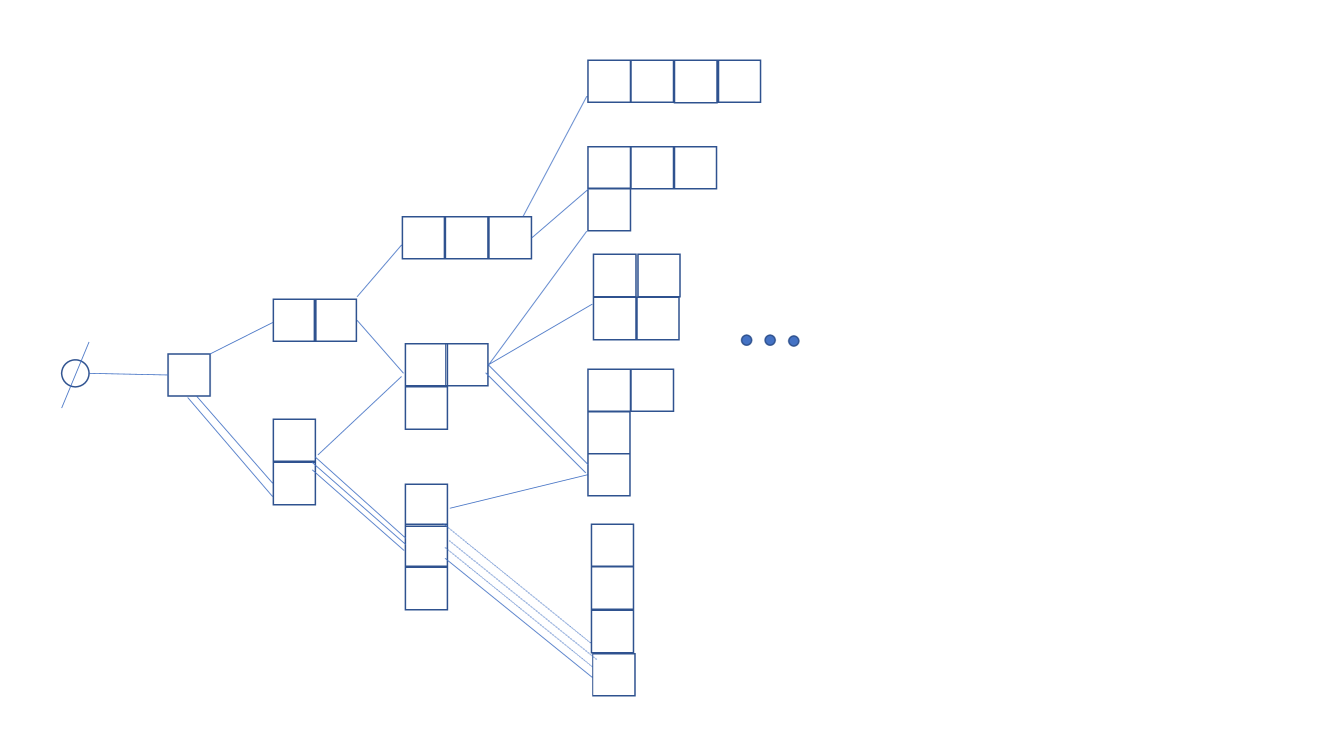
Figure 4. The Kingman graph

It is known (see Borodin and Olshanski [2], Section 4) that the dimension function $\dim_{\operatorname{Kingman}}(\lambda)$ (i.e.the number of ways to get $\lambda$ from $\emptyset$) of the Kingman graph is equal to

$$\dim_{\operatorname{Kingman}}(\lambda)=\frac{|\lambda|!}{|\lambda_{1}|!|\lambda_{2}|!\ldots|\lambda_{l(\lambda)}|!},$$

where $\lambda=\left(\lambda_{1},\ldots,\lambda_{l(\lambda)}\right)$. Thus we obtain

(8.7) $$\operatorname{DIM}_{\theta=0}\left(\Lambda_{n}^{(k)}\right)=n!\prod\limits_{l=1}^{k}\frac{d_{l}^{|\lambda^{(l)}|}}{|\lambda^{(l)}_{1}|!|\lambda^{(l)}_{2}|!\ldots|\lambda^{(l)}_{l\left(\lambda^{(l)}\right)}|!}.$$

The formula just written above enables us to find the ratio of dimension functions in the left-hand side of equation (8.4) explicitly,

(8.8) $$\frac{\operatorname{DIM}_{\theta=0}\left(\widetilde{\Lambda}_{n-1}^{(k)}\right)}{\operatorname{DIM}_{\theta=0}\left(\Lambda_{n}^{(k)}\right)}=\left\{\begin{array}[]{ll}\frac{L^{(1)}}{nd_{1}},&\mu^{(1)}\nearrow\lambda^{(1)},\\ \frac{L^{(2)}}{nd_{2}},&\mu^{(2)}\nearrow\lambda^{(2)},\\ \vdots,&\\ \frac{L^{(k)}}{nd_{k}}&\mu^{(k)}\nearrow\lambda^{(k)},\\ 0,&\mbox{otherwise},\\ \end{array}\right.$$

where $L^{(l)}$ denotes the length of the row in $\lambda^{(l)}$ from which a box was removed to get $\mu^{(l)}$.

Let us find a formula for $\Upsilon_{\theta=0}\left(\widetilde{\Lambda}_{n-1}^{(k)},\Lambda_{n}^{(k)}\right)$. Equation (3.4) gives the multiplicity $\Upsilon_{\theta}\left(\widetilde{\Lambda}_{n-1}^{(k)},\Lambda_{n}^{(k)}\right)$ in terms of the multiplicities $\chi_{\theta}\left(\mu^{(l)},\lambda^{(l)}\right)$. As $\theta\rightarrow 0$, the multiplicities $\chi_{\theta}\left(\mu^{(l)},\lambda^{(l)}\right)$ turn into the multiplicities $\chi_{\operatorname{Kingman}}\left(\mu^{(l)},\lambda^{(l)}\right)$ defined by equation (8.6). We find

(8.9) $$\Upsilon_{\theta=0}\left(\widetilde{\Lambda}_{n-1}^{(k)},\Lambda_{n}^{(k)}\right)=\left\{\begin{array}[]{ll}d_{1}r_{L^{(1)}}\left(\lambda^{(1)}\right),&\mu^{(1)}\nearrow\lambda^{(1)},\\ d_{2}r_{L^{(2)}}\left(\lambda^{(2)}\right),&\mu^{(2)}\nearrow\lambda^{(2)},\\ \vdots,&\\ d_{k}r_{L^{(k)}}\left(\lambda^{(k)}\right),&\mu^{(k)}\nearrow\lambda^{(k)},\\ 0,&\mbox{otherwise}.\\ \end{array}\right.$$

Equation (8.4) follows from equations (8.3), (8.8), and (8.9). Proposition 3.3 is proved. ∎

8.3. Proof of Theorem 2.2

Theorem 2.2 is a corollary of Theorem 3.4. Namely, we apply Theorem 3.4, and take the limit $\theta\rightarrow 0$. As $\theta\rightarrow 0$, the variables

$$\left\{p_{r,l}^{o}(\alpha,\beta,\delta;\theta):\;r\geq 1,\;l=1,\ldots,k\right\}$$

defined by equation (3.10) turn into the extended power symmetric functions $p_{r,l}^{o}(\alpha,\delta)$ defined by

$$p_{r,l}^{o}(\alpha,\delta)=\left\{\begin{array}[]{ll}\sum\limits_{i=1}^{\infty}\left(\alpha_{i}^{(l)}\right)^{r},&r=2,3,\ldots,\\ \delta^{(l)},&r=1,\end{array}\right.$$

and each $P_{\lambda^{(l)}}^{o}(\alpha,\beta,\delta;\theta)$ turns into the extended monomial function $M_{\lambda^{(l)}}\left(\alpha^{(l)},\delta^{(l)}\right)$ defined by equation (2.5). Moreover, the set $\Omega(G)$ is replaced by $\overline{\nabla}^{(k)}$ defined by (2.2). In this way we obtain the integral representation (2.3) for a multiple partition structure. ∎

9. Proof of Proposition 4.1

If $G$ contains only the identity element, then $k=1$, $|G|=1$, and expression (4.2) turns into

(9.1) $$P_{t_{1},n}^{\operatorname{Ewens}}(x)=\frac{t_{1}^{[x]}}{\left(t_{1}\right)_{n}},\;\;x\in S(n),\;\;t_{1}>0.$$

Here $[x]$ denotes the number of cycles in $x\in S(n)$, and $\left(t_{1}\right)_{n}=t_{1}\left(t_{1}+1\right)\ldots\left(t_{1}+n-1\right)$ is the Pochhammer symbol. This measure is a probability measure on the symmetric group $S(n)$, see, for example, Olshanski [25]. Since $P_{t_{1},n}^{\operatorname{Ewens}}$ is invariant under the action of $S(n)$ on itself by conjugations it gives rise to the probability measure $M_{t_{1},n}^{\operatorname{Ewens}}$ on the set $\operatorname{\mathbb{Y}}_{n}$ of Young diagrams with $n$ boxes,

(9.2) $$M_{t_{1},n}^{\operatorname{Ewens}}\left(\lambda\right)=\frac{n!}{1^{r_{1}(\lambda)}r_{1}(\lambda)!2^{r_{2}(\lambda)}r_{2}(\lambda)!\ldots n^{r_{n}(\lambda)}r_{n}(\lambda)!}\frac{t_{1}^{l(\lambda)}}{\left(t_{1}\right)_{n}},\;\;\lambda\in\operatorname{\mathbb{Y}}_{n},$$

where $r_{j}(\lambda)$ denotes the number of rows of length $j$ in the Young diagram $\lambda$.

Consider the general case of an arbitrary finite group $G$ with $k$ conjugacy classes. Since the map $x\rightarrow t_{1}^{[x]_{c_{1}}}t_{2}^{[x]_{c_{2}}}\ldots t_{k}^{[x]_{c_{k}}}$ defines a function which is constant on the conjugacy classes of $G\sim S(n)$, the sum

(9.3) $$\sum\limits_{x\in G\sim S(n)}t_{1}^{[x]_{c_{1}}}t_{2}^{[x]_{c_{2}}}\ldots t_{k}^{[x]_{c_{k}}}$$

can be rewritten as

(9.4) $$\sum\limits_{\Lambda_{n}^{(k)}=\left(\lambda^{(1)},\ldots,\lambda^{(k)}\right)\in\operatorname{\mathbb{Y}}_{n}^{(k)}}\left|K_{\Lambda_{n}^{(k)}}\right|t_{1}^{r_{1}\left(\lambda^{(1)}\right)+\ldots+r_{n}\left(\lambda^{(1)}\right)}t_{2}^{r_{1}\left(\lambda^{(2)}\right)+\ldots+r_{n}\left(\lambda^{(2)}\right)}\ldots t_{k}^{r_{1}\left(\lambda^{(k)}\right)+\ldots+r_{n}\left(\lambda^{(k)}\right)},$$

where $\left|K_{\Lambda_{n}^{(k)}}\right|$ denotes the number of elements of $G\sim S(n)$ in the conjugacy class parameterized by $\Lambda_{n}^{(k)}=\left(\lambda^{(1)},\ldots,\lambda^{(k)}\right)$. This number is given by equation (4.1).

Inserting the expression for $\left|K_{\Lambda_{n}^{(k)}}\right|$ into the sum in (9.4) we rewrite (9.4) as

(9.5) $$n!\left|G\right|^{n}\underset{|\lambda^{(1)}|+\ldots+|\lambda^{(k)}|=n}{\sum\limits_{\lambda^{(1)},\ldots,\lambda^{(k)}}}\frac{\left(\frac{t_{1}}{\zeta_{1}}\right)_{|\lambda^{(1)}|}\ldots\left(\frac{t_{k}}{\zeta_{k}}\right)_{|\lambda^{(k)}|}}{|\lambda^{(1)}|!\ldots|\lambda^{(k)}|!}M^{\operatorname{Ewens}}_{\frac{t_{1}}{\zeta_{1}},\;|\lambda^{(1)}|}\left(\lambda^{(1)}\right)\ldots M^{\operatorname{Ewens}}_{\frac{t_{k}}{\zeta_{k}},\;|\lambda^{(k)}|}\left(\lambda^{(k)}\right).$$

Since

(9.6) $$n!\sum\limits_{m_{1}+\ldots+m_{k}=n}\frac{\left(\frac{t_{1}}{\zeta_{1}}\right)_{m_{1}}\ldots\left(\frac{t_{k}}{\zeta_{k}}\right)_{m_{k}}}{m_{1}!\ldots m_{k}!}=\left(\frac{t_{1}}{\zeta_{c_{1}}}+\ldots\frac{t_{k}}{\zeta_{c_{k}}}\right)_{n},$$

Proposition 4.1 holds true.∎

10. Construction of harmonic functions on $\Gamma_{\theta}(G)$ using harmonic functions on the Jack branching graph. Proof of Proposition 4.2

In this Section we show how a harmonic function on $\Gamma_{\theta}\left(G\right)$ can be constructed from harmonic functions on the Jack branching graph, see Proposition 10.1. Corollary 10.2 from Proposition 10.1 is used to prove Proposition 4.2.

Let $\operatorname{\mathbb{Y}}_{\theta}$ be the Jack branching graph, i.e. the Young graph with the Jack edge multiplicities $\chi_{\theta}(\mu,\lambda)$ defined by equation (3.5). A function $\psi:\operatorname{\mathbb{Y}}_{\theta}\rightarrow\operatorname{\mathbb{R}}_{\geq 0}$ defined on the set of vertices in $\operatorname{\mathbb{Y}}_{\theta}$ is called harmonic on the Jack branching graph if the condition

(10.1) $$\psi\left(\mu\right)=\sum\limits_{\lambda:\lambda\searrow\mu}\chi_{\theta}(\mu,\lambda)\psi(\lambda)$$

is satisfied. We assume that $\psi$ is normalized by the condition $\psi(\emptyset)=1$.

Proposition 10.1.

Let $\varphi_{1}$, $\ldots$, $\varphi_{k}$ be harmonic functions on the Jack branching graph, and let $\tau_{1}$, $\ldots$, $\tau_{k}$ be strictly positive real numbers. Then the function $\varphi:\;\operatorname{\mathbb{Y}}_{n}^{(k)}\rightarrow\operatorname{\mathbb{R}}$ defined by

(10.2) $$\varphi\left(\Lambda_{n}^{(k)}\right)=\frac{\left(\tau_{1}\right)_{|\lambda^{(1)}|}\ldots\left(\tau_{k}\right)_{|\lambda^{(k)}|}}{\left(\tau_{1}+\ldots+\tau_{k}\right)_{n}}\frac{\varphi_{1}\left(\lambda^{(1)}\right)\ldots\varphi_{k}\left(\lambda^{(k)}\right)}{\prod_{j=1}^{k}\left(d_{j}\right)^{|\lambda^{(j)}|}}$$

(where $\Lambda_{n}^{(k)}=\left(\lambda^{(1)},\ldots,\lambda^{(k)}\right)$, and $d_{1}$, $\ldots$, $d_{k}$ are the dimensions of the irreducible representations of $G$) is harmonic on $\Gamma_{\theta}(G)$.

Proof.

We need to show that $\varphi$ defined by (10.2) satisfies the condition

(10.3) $$\varphi\left(\widetilde{\Lambda}_{n-1}^{(k)}\right)=\sum\limits_{\Lambda_{n}^{(k)}\in\operatorname{\mathbb{Y}}_{n}^{(k)}}\Upsilon_{\theta}(\widetilde{\Lambda}_{n-1}^{(k)},\Lambda_{n}^{(k)})\varphi\left(\Lambda_{n}^{(k)}\right),$$

for each $\widetilde{\Lambda}_{n-1}^{(k)}\in\operatorname{\mathbb{Y}}_{n-1}^{(k)}$. Here $\Upsilon_{\theta}$ is defined by equation (3.4). If $\widetilde{\Lambda}_{n-1}^{(k)}=\left(\mu^{(1)},\ldots,\mu^{(k)}\right)$, then the right-hand side of the equation above can be written as

(10.4) $$\sum\limits_{j=1}^{k}d_{j}\underset{\lambda^{(i)}=\mu^{(i)},\;i\neq j}{\sum\limits_{\Lambda_{n}^{(k)}:\;\lambda^{(j)}\searrow\mu^{(j)}}}\chi_{\theta}\left(\mu^{(j)},\lambda^{(j)}\right)\frac{\left(\tau_{1}\right)_{|\lambda^{(1)}|}\ldots\left(\tau_{k}\right)_{|\lambda^{(k)}|}}{\left(\tau_{1}+\ldots+\tau_{k}\right)_{n}}\frac{\varphi_{1}\left(\lambda^{(1)}\right)\ldots\varphi_{k}\left(\lambda^{(k)}\right)}{\prod_{j=1}^{k}\left(d_{j}\right)^{|\lambda^{(j)}|}}$$

This expression can be rewritten further as

(10.5) $$\begin{split}&\frac{1}{\left(\tau_{1}+\ldots+\tau_{k}\right)_{n}}\frac{\varphi_{1}\left(\mu^{(1)}\right)\ldots\varphi_{k}\left(\mu^{(k)}\right)}{\prod_{j=1}^{k}\left(d_{j}\right)^{|\mu^{(j)}|}}\\ &\times\sum\limits_{j=1}^{k}\left(\tau_{1}\right)_{|\mu^{(1)}|}\ldots\left(\tau_{j-1}\right)_{|\mu^{(j-1)}|}\left(\tau_{j}\right)_{|\mu^{(j)}|+1}\left(\tau_{j+1}\right)_{|\mu^{(j+1)}|}\ldots\left(\tau_{k}\right)_{|\mu^{(k)}|},\end{split}$$

where we have used the fact that each of the functions $\varphi_{1}$, $\ldots$, $\varphi_{k}$ is harmonic on the Jack graph $\operatorname{\mathbb{Y}}_{\theta}$ with the multiplicity $\chi_{\theta}$. Since

$$\left(\tau_{j}\right)_{|\mu^{(j)}|+1}=\left(\tau_{j}\right)_{|\mu^{(j)}|}\left(\tau_{j}+|\mu^{(j)}|\right),$$

we see that the right-hand side of (10.4) is equal to $\varphi\left(\widetilde{\Lambda}_{n-1}^{(k)}\right)$. ∎

Let $\psi$ be a harmonic function on $\operatorname{\mathbb{Y}}_{\theta}$. A sequence $\left(M_{n}\right)_{n=1}^{\infty}$ defined by $M_{n}(\lambda)=\dim_{\theta}(\lambda)\psi(\lambda)$ (where $\dim_{\theta}$ is the dimension function on $\operatorname{\mathbb{Y}}_{\theta}$) is called a coherent system of measures on $\operatorname{\mathbb{Y}}_{\theta}$.

Corollary 10.2.

Let $\left(M_{n}^{(1)}\right)_{n=1}^{\infty}$, $\ldots$, $\left(M_{n}^{(k)}\right)_{n=1}^{\infty}$ be $k$ sequences of coherent probability measures on the Jack branching graph $\operatorname{\mathbb{Y}}_{\theta}$. Then the sequence $\left(\mathcal{M}_{n}\right)_{n=1}^{\infty}$ defined by

(10.6) $$\mathcal{M}_{n}(\Lambda_{n}^{(k)})=\frac{\left(\tau_{1}\right)_{|\lambda^{(1)}|}\ldots\left(\tau_{k}\right)_{|\lambda^{(k)}|}}{\left(\tau_{1}+\ldots+\tau_{k}\right)_{n}}\frac{n!}{|\lambda^{(1)}|!\ldots|\lambda^{(k)}|!}M^{(1)}_{|\lambda^{(1)}|}\left(\lambda^{(1)}\right)\ldots M^{(k)}_{|\lambda^{(k)}|}\left(\lambda^{(k)}\right)$$

is a coherent system of probability measures on $\Gamma_{\theta}(G)$.

Proof.

Corollary 10.2 follows immediately from Proposition 10.1, and from the formula

(10.7) $$\operatorname{DIM}_{\theta}(\Lambda_{n}^{(k)})=n!\prod_{j=1}^{k}\frac{d_{j}^{|\lambda^{(j)}|}}{|\lambda^{(j)}|!}\dim_{\theta}\left(\lambda^{(j)}\right)$$

for the number of ways to get $\Lambda_{n}^{(k)}$ from the empty diagram on the branching graph $\Gamma_{\theta}(G)$. ∎

Proof of Proposition 4.2. Write $\mathcal{M}_{t_{1},\ldots,t_{k};\;n}^{\operatorname{Ewens}}$ as in equation (4.4). It is known that $\left(\mathcal{M}_{t,n}^{\operatorname{Ewens}}\right)_{n=1}^{\infty}$ is a coherent system of probability measures on the Kingman graph, i.e. on the Jack branching graph with the Jack parameter equal to zero. Corollary 10.2 implies that $\left(\mathcal{M}_{t_{1},\ldots,t_{k};n}^{\operatorname{Ewens}}\right)_{n=1}^{\infty}$ is a coherent system of probability measures on $\Gamma_{\theta=0}(G)$. By Proposition 3.3 it is a multiple partition structure. Proposition 4.2 is proved. ∎

11. Proof of Theorem 4.3

By Theorem 2.2 the measure $\mathcal{M}^{\operatorname{Ewens}}_{t_{1},\ldots,t_{k};\;n}$ can be represented as

(11.1) $$\begin{split}&\mathcal{M}^{\operatorname{Ewens}}_{t_{1},\ldots,t_{k};\;n}\left(\Lambda_{n}^{(k)}\right)=\frac{n!}{\prod\limits_{j=1}^{k}|\lambda^{(j)}_{1}|!\ldots|\lambda^{(j)}_{l(\lambda^{(j)})}|!}\\ &\times\int\limits_{\overline{\nabla}^{(k)}}M_{\lambda^{(1)}}(\tilde{x}^{(1)},\tilde{\delta}^{(1)})\ldots M_{\lambda^{(k)}}(\tilde{x}^{(k)},\tilde{\delta}^{(k)})P\left(d\tilde{x}^{(1)},\ldots d\tilde{x}^{(k)},d\tilde{\delta}^{(1)},\ldots d\tilde{\delta}^{(k)}\right),\end{split}$$

where $\Lambda_{n}^{(k)}=\left(\lambda^{(1)},\ldots,\lambda^{(k)}\right)\in\operatorname{\mathbb{Y}}_{n}^{(k)}$, $M_{\lambda^{(l)}}\left(\tilde{x}^{(l)},\tilde{\delta^{(l)}}\right)$ are the extended monomial symmetric functions defined by equation (2.5), the set $\overline{\nabla}^{(k)}$ is defined by equation (2.2), and $P$ is a unique probability measure on $\overline{\nabla}^{(k)}$ satisfying (11.1). Our aim is to describe this measure explicitly.

The Kingman representation formula (equation (4.10)), equation (4.4), and equation (11.1) imply that the following condition should be satisfied

(11.2) $$\begin{split}&\frac{\left(T_{1}\right)_{|\lambda^{(1)}|}\ldots\left(T_{k}\right)_{|\lambda^{(k)}|}}{\left(T_{1}+\ldots+T_{k}\right)_{n}}\int\limits_{\overline{\nabla}_{0}^{(1)}}\ldots\int\limits_{\overline{\nabla}_{0}^{(1)}}m_{\lambda^{(1)}}\left(x^{(1)}\right)\ldots m_{\lambda^{(k)}}\left(x^{(k)}\right)PD(T_{1})\left(dx^{(1)}\right)\ldots PD(T_{k})\left(dx^{(k)}\right)\\ &=\int\limits_{\overline{\nabla}^{(k)}}M_{\lambda^{(1)}}(\tilde{x}^{(1)},\tilde{\delta}^{(1)})\ldots M_{\lambda^{(k)}}(\tilde{x}^{(k)},\tilde{\delta}^{(k)})P\left(d\tilde{x}^{(1)},\ldots d\tilde{x}^{(k)},d\tilde{\delta}^{(1)},\ldots d\tilde{\delta}^{(k)}\right),\end{split}$$

where the set $\overline{\nabla}_{0}^{(1)}$ is defined by equation (4.9). Note that the prefactor before the integral in the left-hand side of equation (11.2) can be written as

(11.3) $$\frac{\Gamma\left(T_{1}+\ldots+T_{k}\right)}{\Gamma\left(T_{1}\right)\ldots\Gamma\left(T_{k}\right)}\underset{\delta_{1}+\ldots+\delta_{k}=1}{\underset{\delta_{1}\geq 0,\ldots,\delta_{k}\geq 0}{\int\ldots\int}}\delta_{1}^{T_{1}+|\lambda^{(1)}|-1}\delta_{2}^{T_{2}+|\lambda^{(2)}|-1}\ldots\delta_{k}^{T_{k}+|\lambda^{(k)}|-1}d\delta_{1}\ldots d\delta_{k-1}.$$

The monomial symmetric functions are homogeneous, in particular

$$\delta_{l}^{|\lambda^{(l)}|}m_{\lambda^{(l)}}\left(x^{(l)}\right)=m_{\lambda^{(l)}}\left(\delta_{l}x^{(l)}\right),\;\;1\leq l\leq k.$$

We obtain that condition (11.2) can be rewritten as

(11.4) $$\begin{split}&\int\limits_{\overline{\nabla}_{0}^{(1)}}\ldots\int\limits_{\overline{\nabla}_{0}^{(1)}}\underset{\delta_{1}+\ldots+\delta_{k}=1}{\underset{\delta_{1}\geq 0,\ldots,\delta_{k}>0}{\int\ldots\int}}\left(\prod\limits_{l=1}^{k}m_{\lambda^{(l)}}\left(\delta_{l}x^{(l)}\right)PD(T_{l})\left(dx^{(l)}\right)\right)D(T_{1},\ldots,T_{k})\left(d\delta^{(1)},\ldots,d\delta^{(k)}\right)\\ &=\int\limits_{\overline{\nabla}^{(k)}}M_{\lambda^{(1)}}(\tilde{x}^{(1)},\tilde{\delta}^{(1)})\ldots M_{\lambda^{(k)}}(\tilde{x}^{(k)},\tilde{\delta}^{(k)})P\left(d\tilde{x}^{(1)},\ldots d\tilde{x}^{(k)},d\tilde{\delta}^{(1)},\ldots d\tilde{\delta}^{(k)}\right),\end{split}$$

where $D\left(T_{1},\ldots,T_{k}\right)$ is the Dirichlet distribution defined by its density (4.8), and $P$ is a unique probability measure on $\overline{\nabla}^{(k)}$ satisfying (11.4). Assume that the distribution $P$ is such that

(11.5) $$\tilde{x}^{(l)}=\delta^{(l)}x^{(l)},\;\;l=1,\ldots,k$$

in distribution, and

(11.6) $$\tilde{\delta}^{(l)}=\delta^{(l)},\;\;l=1,\ldots,k$$

in distribution, where $x^{(1)}$, $\ldots$, $x^{(k)}$ are independent with distributions $PD(T_{1})$, $\ldots$, $PD(T_{k})$ respectively, the joint distribution of $\delta^{(1)}$, $\ldots$, $\delta^{(k)}$ is $D(T_{1},\ldots,T_{k})$, and each $\delta^{(l)}$, $l=1,\ldots,k$ is independent from $x^{(1)}$, $\ldots$, $x^{(k)}$. In other words, assume that the joint distribution of $\tilde{x}^{(l)}$, $\delta^{(l)}$ is the multiple Poisson-Dirichlet distribution $PD(T_{1},\ldots,T_{k})$ as in the statement of Theorem 4.3. Then

$$\sum\limits_{i=1}^{\infty}\tilde{x}_{i}^{(l)}=\tilde{\delta}^{(l)},\;\;l=1,\ldots,k,$$

the distribution $P=PD(T_{1},\ldots,T_{k})$ is concentrated on $\overline{\nabla}_{0}^{(k)}$,

$$M_{\lambda^{(l)}}\left(x^{(l)},\delta^{(l)}\right)=m_{\lambda^{(l)}}\left(\delta^{(l)}x^{(l)}\right),\;\;l=1,\ldots,k,$$

and condition (11.4) is satisfied. Theorem 4.3 is proved. ∎

References

- [1] Arratia, R.; Barbour, A.; Tavar, S. Logarithmic combinatorial structures: a probabilistic approach. European Mathematical Society, Zurich, 2003.
- [2] Borodin, A.; Olshanski, G. Harmonic functions on multiplicative graphs and interpolation polynomials. Electron. J. Combin. 7 (2000), Research Paper 28.
- [3] Borodin, A.; Olshanski, G. Representations of the infinite symmetric group. Cambridge Studies in Advanced Mathematics, 160. Cambridge University Press, Cambridge, 2017.
- [4] Bufetov, A.; Gorin, V. Stochastic monotonicity in Young graph and Thoma theorem. Int. Math. Res. Not. IMRN 2015, no. 23, 12920–12940.
- [5] Cuenca, C.; Olshanski, G. Infinite-dimensional groups over finite fields and Hall-Littlewood symmetric functions. Adv. Math. 395 (2022), Paper No. 108087.
- [6] Ewens, W. J. The sampling theory of selectively neutral alleles. Theoret. Population Biol. 3 (1972), .
- [7] Garnet, J. Bounded Analytic Functions. Academic Press, New York, 1981.
- [8] Gorin, V.; Kerov, S.; Vershik, A. Finite traces and representations of the group of infinite matrices over a finite field. Adv. Math. 254 (2014), 331–-395.
- [9] Feng, S. The Poisson-Dirichlet Distribution and Related Topics. Models and Asymptotic Behaviors. Springer 2010.
- [10] Hirai, T.; Hirai, E.; Hora, A. Limits of characters of wreath products of a compact group with the symmetric groups and characters of . I. Nagoya Math. J. 193 (2009), 1–-93.
- [11] Hora, A.; Hirai, T.; Hirai, E. Limits of characters of wreath products of a compact group with the symmetric groups and characters of . II. From a viewpoint of probability theory. J. Math. Soc. Japan 60 (2008), no. 4, 1187–1217
- [12] Hora, A.; Hirai, T. Harmonic functions on the branching graph associated with the infinite wreath product of a compact group. Kyoto J. Math. 54 (2014), no. 4, 775–817.
- [13] Karlin, S.; McGregor, J. Addendum to a paper of W. Ewens. Theoret. Population Biol. 3 (1972), 113–-116.
- [14] Kerov, S. V. Combinatorial examples in the theory of AF-algebras. (Russian) Zap. Nauchn. Sem. Leningrad. Otdel. Mat. Inst. Steklov. (LOMI) 172 (1989), Differentsialnaya Geom. Gruppy Li i Mekh. Vol. 10, 55–-67, 169–-170; translation in J. Soviet Math. 59 (1992), no. 5, 1063–-1071.
- [15] Kerov, S. V. Asymptotic representation theory of the symmetric group and its applications in analysis. Translated from the Russian manuscript by N. V. Tsilevich. With a foreword by A. Vershik and comments by G. Olshanski. Translations of Mathematical Monographs, 219. American Mathematical Society, Providence, RI, 2003.
- [16] Kerov, S.; Okounkov, A.; Olshanski, G. The boundary of the Young graph with Jack edge multiplicities. Internat. Math. Res. Notices , no. 4, (1998), 173–-199.
- [17] Kerov, S.; Olshanski, G.; Vershik, A. Harmonic analysis on the infinite symmetric group. Invent. Math. 158 (2004), no. 3, 551–-642.
- [18] Kingman, J. F. C. Random partitions in population genetics. Proc. R. Soc. London A 361, (1978), 1–20.
- [19] Kingman, J. F. C. The representation of partition structures. J. London Math. Soc. 18 (1978), 374–380.
- [20] Macdonald, I. Symmetric Functions and Hall Polynomials. Oxford Mathematical Monographs. Oxford University Press, second edition, 1995.
- [21] Okounkov, A. Yu. Thoma’s theorem and representations of an infinite bisymmetric group. (Russian) Funktsional. Anal. i Prilozhen. 28 (1994), no. 2, 31–-40, 95; translation in Funct. Anal. Appl. 28 (1994), no. 2, 100–-107
- [22] Okounkov, A. (Shifted) Macdonald polynomials: q-integral representation and combinatorial formula. Compositio Math. 112 (1998), no. 2, 147–-182.
- [23] Okounkov, A.; Olshanski, G. Shifted Schur functions. (Russian) Algebra i Analiz 9 (1997), no. 2, 73–-146; translation in St. Petersburg Math. J. 9 (1998), no. 2, 239–-300
- [24] Okounkov, A.; Olshanski, G. Shifted Jack polynomials, binomial formula, and applications. Math. Res. Lett. 4 (1997), no. 1, 69-–78.
- [25] Olshanski, G. Random permutations and related topics. The Oxford handbook of random matrix theory, 510–533, Oxford Univ. Press, Oxford, 2011.
- [26] Tavar, S. The magical Ewens sampling formula. Bull. London Math. Soc. 53 (2021), 1563–1582.
- [27] Thoma, E. Die unzerlegbaren, positiv-definiten Klassenfunktionen der abzählbar unendlichen, symmetrischen Gruppe. (German) Math. Z. 85 (1964), 40–-61.
- [28] Vershik, A. M.; Kerov, S. V. Asymptotic theory of the characters of a symmetric group. (Russian) Funktsional. Anal. i Prilozhen. 15 (1981), no. 4, 15–-27, 96.
- [29] Vershik, A. M.; Tsilevich, N. V.; The Schur-Weyl graph and Thoma’s theorem. Funct. Anal. Appl. 55 (2021), no. 3, 198–-209.
- [30] Watterson, G. A. The stationary distribution of the infinitely-many neutral alleles diffusion model. J. Appl. Probability 13 (1976), no. 4, 639–-651.