A Prufer-Sequence Based Representation of Large Graphs for Structural Encoding of Logic Networks

Abstract

The pervasiveness of graphs in today’s real life systems is quite evident, where the system either explicitly exists as graph or can be readily modelled as one. Such graphical structure is thus a store house rich information. This has various implication depending on whether we are interested in a node or the graph as a whole. In this paper, we are primarily concerned with the later, that is, the inference that the structure of the graph influences the property of the real life system it represents. A model of such structural influence would be useful in inferencing useful properties of complex and large systems, like VLSI circuits, through its structural property. However, before we can apply some machine learning (ML) based technique to model such relationship, an effective representation of the graph is imperative. In this paper, we propose a graph representation which is lossless, linear-sized in terms of number of vertices and gives a 1-D representation of the graph. Our representation is based on Prufer encoding for trees. Moreover, our method is based on a novel technique, called $\mathcal{GT}$-enhancement whereby we first transform the graph such that it can be represented by a singular tree. The encoding also provides scope to include additional graph property and improve the interpretability of the code.

I Introduction

Graph-based machine learning have seen a surge of research, recently, driven by the prevalence of graphs in the real world systems. In such environments, either the data naturally occur as graphs like in biological networks, or the interactions are modeled through graphs as in social networks. The graph based ML have been applied to varied of problem setting with a range of unique approaches [1]. While ML has gained stupendous proficiency in its tools and techniques as well as huge success in its application, its downside lies in the fact that the basic mathematical operations, that it relies on, necessitates the data to be in a structured format, which may be a feature vector or and an image grid. However, a graphical data is inherently not structured. So, most of the graph-based ML approaches aim at capturing maximum relevant information in a structured format. We next discuss the present works and the different problem setting and approaches.

The real world environment which are represented by graph vary widely in the nature of the graph, the kind of interactions and also their sizes from large graph representing systems like VLSI circuits to extra large like those representing social network. Hence these factors determine the problem setting and approaches. The approach taken also is determined by the precision demanded in terms of the features for ML2 and the scope of representing the graph which is constrained by its size . Although there are many problem setting looked at so far [1], the two generic problem setting has evolved around whether we are interested in obtaining the information about a node or the graph as a whole. While most of the research is focused on the former, the later has fewer solutions in literature. One of the reasons for this is it is challenging to represent the entire graph because of its complexity as well as its size. A number of surveys are available in the literature which focus on three basic approaches: (i) graph embedding [2, 3], (ii) representation learning [4], and (iii) geometric deep learning [5]. Graph embedding aims at representing the graph as a vector [3] or as a set of vectors [2]. The properties are based on local proximity, which are either manually defined or extracted in a automated fashion. The latter belongs to the class of representation learning frameworks where feature formulation is automated using ML or matrix factorization [4]. Geometric deep-learning tools for graphs are aim at applying deep learning tools like convolutional neural nets (CNN) or recurrent neural network (RNN). Vector representations have mostly been used in a node-centric setting where a node is represented by a low-dimensional vector. They are mostly used for node classification or link prediction [6, 7]. Geometric deep learning are based on one of the two techniques, spectral [8] or spatial approach [9]. Spectral analysis have the following major bottlenecks [9]: (i) they are valid only for undirected graphs, (ii) applicable only to graphs with similar size and structure, and (iii) learning is mostly based on the weights of the vertices of the graphs. A few works aim at capturing full graph embedding/learning, e.g., graph kernel or graph neural network (GNN) [10]. However, none of these preserve the graph structure, or are applicable to large graphs. Although CNNs based on spatial analysis have been used to handle arbitrary graphs, complete structure preservation is still a concern [9].

Recently, in the field of integrated circuits, various methods have been employed for efficient application of ML and deep learning tools [11, 12, 13, 14, 15]. One of the rich source of graph based data is the graphical structure of the logical circuits called circuit-graphs. Circuit-graphs are directed acyclic graphs (DAG) representing combinational or scan-based logic circuits. It has been seen that the structural features of the circuit-graph can be used to infer the some property of the circuit [16]. Since devising the structural features in laborious some ML based techniques to learn the structural features would expedite the process. However, such type of graph based learning has not been addressed in any of the previous methods. A major requirement here is the need for an effective graph representation for which there is no proper existing method.

In this paper, we propose a representation of graphs, which are large, and which fulfill the following properties that are required for the afore-mentioned problem setting. Firstly, it is lossless. The structure of the graph is preserved in the proposed representation. Secondly, it is linear sized in terms of the number of vertices. Hence it is convenient to store large sparse graphs. Thirdly, we propose a 1D representation of graph. Such a representation, we believe would be convenient for ML based applications since most of the ML tools work on vectors of 2-D grid data.

We introduce a novel encoding technique for this purpose. The encoding is lossless and is based on a very old but not fully explored, graph theoretic concept known as Prüfer sequence [17]. This sequence was first used in 1918 to prove Cayley’s formula, which was used to count the number of possible spanning trees in a graph with a given number of vertices. The classical Prüfer code can be used for encoding trees only; however we are concerned with graphs. For encoding of a graph, we need to represent it with a tree. So, we propose a technique called graph-to-tree enhancement ($\mathcal{GT}$-enhancement), for this purpose. We call such a tree, which represents a graph through $\mathcal{GT}$-enhancement, a g-tree. We present two approaches for $\mathcal{GT}$-enhancement. The first approach is based on DFS traversal and relies on some additional operations to obtain a desirable g-tree. In the second approach, we have simpled the method by introducing a novel graph traversal technique called SCESOR. the Further, we report new properties of Prüfer codes and discuss methods for improving interpretability and preserving the edge directions. We also discuss Prüfer codes in the light of making them learnable.

The rest of the chapter is organized as follows. The motivation and methodology appear in Section II and Section III, respectively. Section IV and Section V report the two methods that can be used to obtain a g-tree. Section VI provides a discussion on the properties of Prüfer code. Conclusions and future work appear in Section VII.

II Motivation

We will discuss the motivation highlighting three aspects. Firstly we will discuss effectiveness of Prüfer codes in representing large graphs representing real world systems. Secondly, that although prufer sequence is applied only to trees, it can be easily applied to graphs by representing a graph as a single tree through the proposed methods of $\mathcal{GT}$-enhancement, which is discussed in later section. Thirdly, we give an illustrative example to demonstrate the capability of a Prüfer sequence to preserve the entire structure of a circuit-graph such that the structure to the graph can be regenerated from the prufer code.

(a) Example labeled tree.

(b) Prüfer code of the tree in Figure 1(a)

Figure 1: Example of Prüfer code of a tree.

As mentioned before, the aim of this paper is to devise a representation of the graph which completely preserves the connectivity between the vertices. However, this would be difficult for large graphs since it would require large memory. For example an adjacency matrix would require $n^{2}$ space for a graph of size $n$. Any effort to lessen the size would mean compromising on the connectivity information which we do not want. An interesting and favorable, observation about the graphs, that appear in real world, is that they are typically sparse graphs. This implies that for a graph $G(V,E)$, where $V$ is the vertex set and $E$ is the edge set of $G$, $|E|\ll|V|^{2}$. In general, in sparse graphs $|E|=\mathcal{O}(|V|)$. In fact, for most of the digital test benchmark circuits [18, 19], $|E|$ is not more than $2\times|V|$. Thus, a representation of the connections (edges), as a series of edges would significantly shrink the size of the code. A straight forward way of lossless representation is to consider all the possible vertex-pair and mark those which are connected as in done in adjacency matrix. But, here we want to keep only the marked vertex pairs (edges) and refrain from retaining the rest of the vertex pairs in our code. The Prüfer sequence provides a elegant method for such representation. A Prüfer encoding represents a labeled tree of $n$ nodes (and hence having $n-1$ edges) by a string of vertex-labels whose length is $n-2$. Figure 1 shows an example of a Prüfer code of a tree. A labeled tree with six vertices is shown in Figure 1(a) and its corresponding Prüfer code is shown in Figure 1(b). The algorithm for encoding the tree and decoding it is discussed in the next section. We will also discuss how each vertex label represents an edge in later section.

(a)

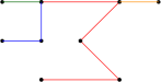
(b)

Figure 2: Graphs with large number of tree-partitions. Top: (a) Sparse graph with 25 vertices 32 edges and 9 tree partitions ; (b) Dense graph with 5 vertices 8 edges and 4 tree partitions. Left: the corresponding g-trees.

Figure 3: An illustration of Prüfer code for the circuit-graph representing the benchmark circuit s27, and reconstructing it from the Prüfer code.

Although prufer encoding elegantly solves a major issue, the problem is yet not entirely solved because Prufer apply only to trees, that i.e., only connected acyclic undirected graphs.

A simple extension of Prüfer codes to graphs would be to partition it into a set of trees so that the graph can be represented as the corresponding set of Prüfer codes for individual trees. This problem does not,however, serve the purpose. The problem of partitioning the edge set $E$ of a graph $G$ into minimum number ($k$) of trees is known to be NP-hard [20]. Moreover for sparse graphs, even $k$ can be very large (Figure 2(a)). Also if the (sub) graphs are dense, the number of trees could be large (Figure. 2(b)). For a complete graph $K_{n}$, the minimum number of tree-partitions is $\lceil n/2\rceil$. So, the number of prufer codes required to represent a graph being close to $|V|$, would be of no value. So, we need a method which completely obviates the need of such huge number of codes. We do so by enhancing the graph into a tree by addition more vertices. This method is called $\mathcal{GT}$-enhancement. The tree is called a g-tree. Also, the $\mathcal{GT}$-enhancement of $G$ preserves the number of edges of $G$ in g-tree. Thus, the size of the Prüfer code of a g-tree is $|E|-1$.

An illustration of the preservation of structural property of a graph is shown in Figure 3. Here, we have taken a circuit-graph as an example and have shown its prufer code and its reconstruction. We have considered an ISCAS’89 [18] benchmark circuit s27 for this purpose. The netlist and the corresponding circuit diagram is shown in Figure 3(a) and Figure 3(b), respectively. The circuit-graph generated from the netlist is given in Figure 3(c). Note that the graph has two cycles. $\mathcal{GT}$-enhancement, which adds two vertices $8^{1}$ and $10^{1}$, creates the g-tree shown in Figure 3(d). The tree is then encoded by a Prüfer sequence as shown in Figure 3(e). The tree structure can be completely reconstructed as shown in Figure 3(f).

In summary, we propose a new encoding scheme for digital networks based on Prüfer sequence which has the following useful properties:

1. it is lossless, i.e., captures the structure of the entire graph;

2. it is memory efficient; the size of encoding is $\mathcal{O}(|V|)$;

3. the representation can be expressed as a single string of vertex labels;

4. it provides an efficient 1-D representation suitable for machine-learning tools;

5. the encoding can be computed in time linear in the size of the graph.

6. it provides scope improve interpretability and also to preserve additional properties of the graph like the directions on edges for DAGs.

III Methodology

In this section we will briefly look at the Prüfer encoding of a tree. We will also introduce the g-tree and show how Prüfer encoding can be applied to it.

III-A Prüfer-Code

Consider a tree, $T$, with $n$ vertices. The simplicity of Prüfer encoding method through the tree can be easily recovered is primarily because it set the following constraints regarding the labels attached to the nodes:

Constraint 1.

The vertices of $T$ are labelled sequentially as {‘$1$’, ‘$2$’, $\cdots$ ‘$n$’}.

Constraint 2.

The vertices of $T$ are comparable such that {‘$1$’ $<$ ‘$2$’ $<$ $\cdots$ $<$ ‘$n$’}.

The steps to encode $T$ is given in Procedure 1.

1:Fetch a single degree vertex, $v$, with the smallest label. Delete $v$.

2:Write the label of the neighbour of $v$ to the right of the code.

3:Repeat Step 2 until only two vertices remain in the tree.

Procedure 1 Encoding: tree-to-code

Consider a Prüfer code of $T$: $c_{1},c_{2},\cdots,c_{m}$; we make the following observation:

Observation 1.

$n=m+2$.

Observation 2.

The degree of a vertex is one more than the number of times the label of a vertex appears in the code.

Corollary 1.

Labels of single-degree vertices do not appear in the code.

The steps for decoding Prüfer code are given in Procedure 2.

1:Initialize a variable $k$ to 1.

2:Compute: $n\leftarrow m+2$; labels $\leftarrow$ {$1\cdots n$}. $\triangleright$ Observation 1.

3:Compute the degree of each node. $\triangleright$ Observation 2.

4:Fetch a single-degree vertex, $v$, with the smallest label. Set ($v,c_{k}$) as an edge of the tree.

5:Decrement the degree of $v$ and $c_{k}$; increment $k$.

6:Repeat Step 4 and Step 5 until all vertices have degree 0, except a pair with degree 1. $\triangleright$ These form the last edge of the tree.

Procedure 2 Decoding: code to tree [21]

A linear-time encoding and a decoding algorithm for Prüfer sequence are given in [22]. Next we will see in what way the two constraints defined on the labels aid in the decoding process. Firstly we decode the number of vertices, $n$, in the tree through the formula given in Observation 2 in step 2, of Procedure 2). Due to the constraint 1 we are able to decode the labels of the vertices . The second constraint enforces a particular sequence of the labels, which is defined by the integer value of the labels. So, this constraints makes it possible to iteratively decode tree.

It is important to note here, that although we could retrieve the information of the label of the vertices though Constaint 1, some information about the labels can also be obtained from the code it self. Precisely stating, the labels of those vertices which are non-pendant are present in the code from Observation 2. So, if need we can relax the first constraint. In such case we need to keep the label information of pendant vertices Corollary 1) in a separate list. Since this list will be required to decode the tree from the code. This is important because in case of g-trees, which we discuss next and is the prime aspect of this paper, we are required to relax the first constraint.

III-B $\mathcal{GT}$-Enhancement and Encoding of g-tree

As discussed earlier we see that the best way to extend prufer encoding scheme to graphs would be to alter the graph such that all the connectivity information of the graph can be embedded in a single tree. So, in this section we discuss the proposed technique of altering a given graph G(V,E) into a single tree so that the prufer encoding of the graph is possible. We call this method $\mathcal{GT}$-enhancement and the tree so obtained is called a g-tree. The complete connectivity information about the graph is preserved in the g-tree by preserving the edges of the graph. We know that a tree is an acyclic graph. So, we convert the graph in a tree simply by removing all the cycles in the graph but without removing the edges. This is done through the proposed technique of vertex-split which is the central operation in $\mathcal{GT}$-enhancement. As the name suggest, the vertex which is part of a cycle is split into two, so we make the graph acyclic by actually breaking the cycle at a vertex. Next we will elaborate on vertex-split operation.

A vertex-split operation on a vertex $v$ splits or replicates the vertex such that a copy of the vertex $v$ (call it $v^{1}$,) is added to the graph. We call this new vertex $v^{1}$ as a split-vertex. Among the edges incident on $v$, some of the edges are altered by making them incident on its split-vertex $v^{1}$, such that the cycle formed because of any of these edges is no longer present. In this paper we propose two methods of $\mathcal{GT}$-enhancement. The methods differ in the way the graph is traversed and also the way vertex-split operation is performed. The vertex-split considers different set of edges to the altered as will be discussed later.

The $\mathcal{GT}$-enhancement of $G$ do not add any new connection/edge to the graph, so the g-tree obtain has the same number of edges as the original graph $G$ that is $|E|$. So, the number of vertices in the g-tree is $|E|+1$. Now, since $G$ originally had $|V|$ number of vertices, the number of additional vertices in the g-tree is $|E|+1-|V|$.

We have seen how the Constraint 1 is taken care of by considering a separate list of labels of pendant vertices. We call this list L. Next we will discuss the labelling scheme for the vertices so that the Constraint 2 made by the prufer encoding scheme is taken care of. Let the g-tree be denoted as a tree $T_{g}$ with vertex set $V^{T}$ and edge set $|E^{T}|$. Let the set of new vertices be $V^{\prime}$.

So, $V^{T}=V\cup V^{\prime}$ and is equal to $|E|$. Let $n$ denote the number of vertices in $T_{g}$, $n_{1}$ denote the number of vertices in the original graph and let $n_{2}$ denote the number of new vertices added. So, $n=n_{1}+n_{2}$ and $n_{2}=|E|+1-|V|$. So, for labelling the tree $T_{g}$, firstly label of the vertices in $V$ are preserved as {‘$1$’ $\cdots$ ‘$n_{1}$’}. Now, a vertex in the graph can ve vertex-split to more than one vertices during $\mathcal{GT}$-enhancement, so when any vertex $v$ with label $l$, where $l$ in an integer, is replicated into $k$ additional vertices, we label as $l^{1},l^{2},\cdots,l^{k}$. In order to preserve Constaint 2, which enforces some ordering among the vertex labels, while encoding $T_{g}$ with a Prüfer code, the labels of these vertices are considered in the order $l<l^{1}<l^{2}<\cdots<l^{k}<$$L+1$ .

Next we discuss the process of decoding the labels from a given prufer encoding of $T_{g}$. The Constraint 1 partially holds for $T_{g}$, since it is true only for $n_{1}$ vertices. So, if the information about $n_{1}$ is known, the labels of these vertices can be computed. However, since we have added new verices here, $n_{1}$ cannot be directly computed. The only information we can come is the value of $n$ (Observation 1). Next, we need to compute $n_{2}$ from which we get the value of $n_{1}$ . Now, to compute $n_{2}$ we need to know the information about the labels of the vertices in $V^{\prime}$. However, for Corollary 1, not all labels appear in the prufer cod. So as discussed earlier from the list $L$ and prufer code be obtain the labels of vertices in $V^{\prime}$ and also its size $n_{2}$.

In the next section, we discussed the two approaches to $\mathcal{GT}$-enhancement. As we earlier, a drawback of this technique is the we need to store an additional list. So, The first method aims at reducing the list $L$ such that $|L|\ll|E|$. The second method completely obviates the need to store the additional list. The second method produces the g-tree where all the additional vertices are of degree two and the labels of vertices in $V^{\prime}$ appear in the code; thus the Prüfer code thus obtained completely represents the graph.

IV Tree-Partition Based $\mathcal{GT}$-Enhancement

In this method, representing an undirected graph by a tree is realized by partitioning the edges of the graph into trees. Thereafter, the individual trees are joined to from a single tree.

IV-A Proposed Approach

Since the problem of finding a minimum tree-partition of a graph $G$ is hard [20], we follow a greedy approach based on depth-first search (DFS) [23] traversal of $G$. DFS of an undirected graph produces a spanning tree $T_{DFS}$; the edges of this tree called are tree-edges and they form the primary partition. The rest of the edges of the subgraph $G^{c}=G\setminus T_{DFS}$ are called back edges. While the DFS spanning tree is implicitly constructed during the traversal, the residual graph $G^{c}$ is often found to be disconnected. The secondary partitions, which are formed by the back edges of $G^{c}$, are called be-trees and belong to one of the following:

1. Class-1 back-edge tree (be-tree-1): These are trees formed by the back edges between the vertices, which have already been visited once.

2. Class-2 back-edge tree (be-tree-2): These are trees formed by the back edges between the vertices, which have already been visited twice: by the DFS-tree and also by a be-tree-1.

3. $q^{th}$ class back-edge tree (be-tree-q): The trees formed by the back edges between the vertices that have already been revisited $q-1$ times, are called be-tree-q.

Note that the DFS-traversal usually yields a number trees for each class. For a given class $i$, all trees in be-tree-i are independent to each other since they have no vertex in common. The be-trees that are non-independent to a given $k^{th}$ be-tree-1, are said belong to the same family, $f_{k}$. Thus, the edges of the graph are partitioned into a spanning DFS-tree and a set of families of non-independent trees.

Example: Figure 4(a) shows an example graph, where the DFS-tree is shown in red. The decomposition consists of one family of be-trees with two classes: be-tree-1 (blue) and be-tree-2 (green). Also note that in Figure 2(a), the graph has eight families of be-trees.

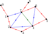
Figure 4: Exmple graph showing the DFS-trees and the secondary partitions.

Next we look at the way the process of $\mathcal{GT}$-enhancement is applied in this method. Given a graph $G(V,E)$ and the set $P$ of secondary partitions, for each partition in $P$, a join vertex ($v_{join}$) is specified. $G$ is decomposed into a g-tree, $T_{g}$, based on $P$ and their join vertices. Each vertex in $V$, belongs to the primary partition. For every vertex $v$ that belongs to some secondary partition $P_{j}$, a vertex-split operation (refer to Figure 7(a)) is performed. The vertex $v$ is split into a split-vertex $v^{P_{j}}$ for every partition $P_{j}$ where it belongs to, such that the edges of $G$ that belong to $P_{j}$ and were incident on $v$, become incident on $v^{P_{j}}$. However, if this vertex is a join-vertex of a partition, its replica for that partition is not created. Thus, the tree $T_{g}$ is formed by the trees for each partition in $P$, each tree sharing a common vertex with the spanning tree at its join vertex. We called this tree DFS-Partition-tree and denote it as $T^{DP}_{G}$. The labeling methodology for the new vertices was described previously in Section III.

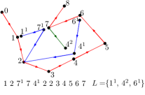
Figure 5: $\mathcal{GT}$-enhancement: g-tree of the example graph. The prufer code and the list L is also shown in the figure.

Example: On performing $\mathcal{GT}$-enhancement on the graph in Figure 4, we obtain the resulting graph as shown in Figure 5.

As shown in Figure 5, there are there pendant split-vertices in the g-tree. So, we need to store their label in the list L. So, next we will look at some operations that can be incorporated in the traversal such that the size of L can be reduced.

IV-B Reducing the size of the list L

Firstly we will see a method to reduce the number of be-tree classes. Since the number of split-vertices is governed to the number of be-tree classes that it belongs to, so this process is favorable at reducing the number of labels that needs to be possibly stored. We call this method as edge-swap and is explained as follows. Consider a pair of vertices, $u$ and $v$, of $G$ such that they are connected by an edge $e$ and also by two paths $p_{dfs}$ and $p_{be1}$. Suppose DFS exploration, traverses the path $p_{dfs}$, including it in the DFS-tree, such that $v$ is visited before $u$. Let $p_{be1}$ be assigned to be-tree-1, $b_{1}$. We define two special edges:
Cycle-edge: At some instant during the traversal when vertex $u$ is being processed, let edge $e$ be a back edge from $u$ to $v$. Since it will introduce a cycle in $b_{1}$, it is assigned to be-tree-2. Such an edge is called a cycle-edge.
Swap-edge: Now, suppose there exists a tree-edge $e_{s}$, in the path $p_{dfs}$, which does not form a cycle with any be-tree-1. Then the edge $e_{s}$ is swapped with $e$; $e_{s}$ is then called a swap-edge for the cycle-edge $e$.
Edge-swap: An edge-swap between the cycle-edge $e$ and its swap-edge $e_{s}$ enables $e$ being assigned to a tree-edge and $e_{s}$ being assigned to be-tree-1. A new class of be-tree for the cycle-edge $e$ is thus avoided by an edge-swap operation. Note that an edge-swap, modifies the DFS-tree, without disconnecting it.

Example: Consider the graph in Figure 4; edge (7-4) and edge(5-6) would be a cycle-edge and swap-edge, respectively. The resulting graph is shown in Figure 6.

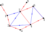
Figure 6: Edge-swap

There are scope to further reducing the list $L$ by taking care of how we form g-tree so that we can smartly handling the labels. Because reducing $L$ imply ensuring that the new labels to point to non-pendant vertices. So, the following two operation exploit this to reduce the size of L:

1. Choice of join-vertex: It is so chosen that it becomes a pendant vertex of the be-tree and the DFS-tree (if possible);

2. Label-swap: The replicas of a vertex in $v$ have similar labels; so exchanging the labels does not change the structure of $G$. The operation label-swap is applicable to a pair of vertices $(v,v^{r})$ with corresponding label $(l,l^{r})$, where $v^{r}$ is a replica vertex of $v$, $v$ is a non-pendant vertex and $v^{r}$ is a pendant vertex. In such case their labels are swapped. So, the label $l^{r}$ now points to a non-pendant vertex and hence it does not need to be stored. So, this operation decreases the size of $L$.

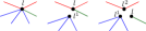
(a) Vertex split with label-swap

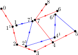
(b) g-tree for the graph in Figure 4 & its Prüfer sequence

Figure 7: g-tree and label-swap operation

Example: The Figure 7(a) depicts label-swap. Also in Figure 7(b), label-swap is performed for the vertex with label “1”. The vertex with label “5” is chosen as join-vertex since it is pendant in both the trees it belongs to. Hence, after all operations, the list $L$ reduces to $\phi$. The corresponding Prüfer sequence is shown in the figure.

IV-C Implementation

In this section, we discuss the outline of our implementation on benchmark integrated circuits [18, 19]. Since scan-based circuits are envisaged as directed acyclic graphs, we first label their nodes in topologically-sorted order [24] and run a single DFS-traversal, considering it as an undirected graph (directions can be retrieved from the labels). Also, the successors of each vertex are visited in the increasing order of their labels. When an edge $e(u,v)$ is discovered, it is (i) assigned to a particular partition by an operation called add-edge (described later), or (ii) added to the list of cycle-edges, or (iii) assigned to a partition (add-edge) if it is already marked as a cycle-edge and has not yet been swapped. When an edge is backtracked, we check whether it is suitable for swapping with a swap-edge in the list. Lastly, once all the edges emanating from a vertex are processed, vertex-splitting along with label-swap is performed on it if needed.

During each successive iteration of the DFS-traversal, search is made to explore an unvisited vertex, and if found, the connecting edge is added to the DFS-tree. Similar implicit exploration cannot, however, be performed to extract be-trees. A pair of edges in a be-tree, or the edges of the successive classes in a family of be-trees, could be discovered during two independent iterations. Thus, to keep track of be-trees, we record the following entities, which are updated whenever a new back-edge is discovered: (i) tree index: every back-edge that does not share a common vertex with any other be-tree formed so far, or form a cycle with the adjacent be-trees, is considered a new be-tree with one-higher index; (ii) vertex-attribute for each vertex $v$ (tree-index list $\mathcal{T}_{v}$): a ordered tuple of indices of different classes of be-trees to which the vertex belongs, and (iii) edge-attribute for each edge e ($c_{e}$): the be-tree class index. $\mathcal{T}_{v}[c_{e}]$ gives the tree-index of the $c_{e}^{th}$ class.

TABLE I: Results on logic circuits in ISCAS’89 and ITC’99 benchmark-suites.

Circuit	#vertices	#edges	Prüfer code	#extra_	#be_	#edge_	#vertex	#label_	CPU-time
			length	labels ($|L|$)	trees	swap	_split	swap	in sec.
ISCAS’89 benchmark circuits [18]
s5378	3206	4435	4434	27	2	1	1230	606	7.76
s9234	6094	8235	8234	292	4	25	2142	1048	15.29
s13207	9441	12048	12047	450	4	14	2608	1184	24.56
s15850	11067	14380	14379	568	4	10	3314	1594	28.74
s38417	25585	33969	33968	1202	4	4	8385	4535	77.78
s38584	22447	34497	34496	2325	4	5	12051	5628	125.77
ITC’99 benchmark circuits [19]
b13s	392	601	600	0	2	7	210	111	1.12
b14s	5020	9862	9861	1324	3	26	4843	1881	40.88
b15s	9343	19068	19067	2534	3	39	9726	3909	87.38
b17s	25615	52447	52446	7282	3	42	26833	10175	307.35
b20s	9909	19555	19554	2739	3	21	9647	3620	98.39
b21s	10293	20300	20299	2387	3	46	10008	3871	104.73
b22s	15836	31304	31303	4105	3	11	15469	5856	158.33

add-edge: When a unvisited back edge $e(u,v)$ is encountered with tree-index lists $\mathcal{T}_{v}$ and $\mathcal{T}_{u}$, $c_{e}$ is computed from the two lists such that it does not form a cycle with any of the trees to which $v$ and $u$ belong. Thereafter, it is assigned to a be-tree by updating the lists depending on the following three cases; (i) union of two be-trees: Suppose $e$ connects two back-edges $e_{1}(v,w_{1})$ and $e_{1}(w_{2},u)$, each belonging to distinct be-trees with tree-indexes $i_{1}$ and $i_{2}$, respectively, but both having the same tree-class. In such a case, the three edges are assigned to a single be-tree having tree-index $i_{1}$. This is done by treating the tree-indices as disjoint sets. Using the disjoint-set data structure, we perform union($i_{1}$, $i_{2}$); (ii) if only one of the two vertices belongs to a unique class of be-tree, the edge $e$ is assigned to that be-tree; (iii) lastly, if it does not fall into the above two cases, it creates a new be-tree as explained above.

The time complexity of the algorithm is $\mathcal{O}(|V|+|E|)$.

IV-D Results on Benchmark Circuits

Results for ISCAS’89 and ITC’99 benchmark-suites are shown in Table I. The experiments were carried out on an Intel Xeon 3.00-GHz $\times$ 4 processor with 8GB memory. Each of the benchmark circuits corresponds to the netlist of a digital logic circuit, where the input-ports/output-ports, logic gates, and memory cells are represented as vertices, and the interconnections among them, as edges, of a directed acyclic graph. The circuit-name, the number of vertices, and edges are given in Columns 1, 2 and 3, respectively. These graphs are very sparse as the edge-count is just around two times of the vertex-count. The length of Prüfer code is given in Column 4. The required number of extra-labels $(L)$ is given in Column 5, which is much less than the number of edges. The highest-index of be-trees is given in Column 6, and the number of edge-swaps is given in Column 7. The number of vertex-splits is shown in Column 8, and out of it the number of vertices whose labels are swapped, is shown in Column 9. The CPU-time needed to encode the circuit using Prüfer-sequence is reported in Column 10, in seconds.

V SCESOR $\mathcal{GT}$-Enhancement

The previous method of tree-partition based method for $\mathcal{GT}$-enhancement is designed solely too meet the purpose of converting the graph the g-tree by breaking every cycle by applying the method of vertex-split. It accomplishes the task through a single DFS traversal taking linear time. The propensity to fulfill the primary objective have made way to some pitfalls related to optimization of various factors. These are discussed as follows.

1. The Prufer sequence is not enough to decode the graph. As seen in Table I, although the methods tries to reduce the size of the list $L$, for almost all the circuit-graphs, it could not entirely preclude its necessity. Clearly, for decoding the graph, this methods can not solely rely on the Prufer code. The graph traversal process was not exploited fully to meet this end since we just followed the conventional ”dept-first” approach. From ML point of view, a single string would be more convenient for good representation of data. However, this method do not consider it as one of the primary objectives.

2. Supplementary operations required to reduce the size of $L$. The vertex-split operation of the this method of $\mathcal{GT}$-enhancement do not target to ensure that the new vertices added are non-pendant. It relies on a set of operations like label-swap or edge-swap. These operations lends undesired complexity to the algorithm.

3. In the cases where a vertex has high degree and that of the most of its neighbors are two, then the number of single-degree nodes which cannot be label-swapped could be large. An instance of this is shown in the Figure 8. The sub-figure 8(a) shows a sub-graph of an instance of such case. The edges belonging to the DFS-tree is shown in red and the edges belonging to a be-tree are shown in blue. Sub-graph 8(b) shows the g-tree obtained by the tree-partition based method. As shown in the figure, there are three pendant split-vertices which can not be label-swapped. This mandates their appearance in the list $L$. Thus making the need of the list $L$ unavoidable. We observe that such split-vertices can be avoided even for such tricky cases by following a different method of traversal and vertex-split through which we arrive at a distinct g-tree where the split-vertices and no longer pendant. This is shown in sub-figure 8(c). This g-tree is obtained by the second method of $\mathcal{GT}$-enhancement called SCESOR $\mathcal{GT}$-enhancement. We will now discuss this method.

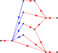
(a)

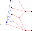
(b)

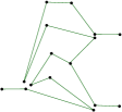
(c)

Figure 8: (a) Sub-graph showing special case; (b) Vertex-split by tree-based $\mathcal{GT}$-enhancement showing three new pendant vertices that can not be label-swapped; (c) Better method of $\mathcal{GT}$-enhancement with no new pendant vertices

The second method of $\mathcal{GT}$- enhancement overcomes these shortcomings. We call this method Seek-Clear-Edge-and-Split-On-Revisit (SCESOR) $\mathcal{GT}$-enhancement. This method maintains that any split-vertex that is added during $\mathcal{GT}$-enhancement is always of degree two. Thus, this method obviates the need for the list $L$. Thus, g-tree can be represented by a single Prüfer code. Furthermore, the method is much simpler to implement. The SCESOR $\mathcal{GT}$-enhancement involves processes:

1. Seek-clear-edge graph traversal.

2. Split-on-revisit of every vertex.

We will discuss each of these process in the following sections.

V-A Seek-Clear-Edge (SCE) Traversal

Here we propose a novel traversal technique which is called Seek-Clear-Edge traversal or SCE traversal. The two classical graph-traversal algorithms, which is as DFS and BFS (breadth-first- search), follow an exploration method that is vertex-centric. The term “search” refers to visiting the vertices sequentially; where the search techniques, which is either “depth-first” or “breadth-first”, refer to the vertices. In contrast, traversal scheme we propose edge-centric; where the exploration will be guided by edges rather than vertices. The SCE-algorithm of a graph $G$ is as follows. Starting from a vertex $v\in G$,an unvisited edge adjacent to $v$, $e^{1}(v,w)$ is visited (flagged). Iteratively, the next unvisited edge adjacent to $w$ is visited. During the traversal, when no unvisited/clear adjacent-edge is available from the current vertex $u$, then the algorithm backtracks to its parent vertex $u_{p}$. If there is any unvisited edge adjacent to $u_{p}$, it is iteratively visited, and the process is continued until all edges in G are flagged.

This traversal algorithm differs with the classical approach in the following ways:

1. A vertex is treated the same; both when discovered for the first time or is when revisited.

2. Backtrack from a vertex only when all its adjacent edges have been visited.

3. Its follows dept-first approach but goes deeper than DFS since its backtrack criteria is fully relaxed.

4. Unlike DFS, here all the edges are tree-edges and so there are no back-edges.

The central idea of this traversal algorithm is that at any instance during the traversal, when a clear edge is available from the current vertex, the edge is visited. Thus, the traversal is regulated by the availability of clear adjacent edges and not by the vertices as typical of the classical traversal process.

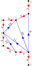
(a) DFS

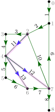
(b) SE

Figure 9: The graph in Fig. 4 is redrawn here to show the difference in the sequence of edge-traversal. Three edges are shaded in (b) to highlight their difference.

An example of the traversal on the graph in Fig. 4 is given in Fig. 9. The graph is redrawn for clarity. The edge-labels depict the sequence number in which the edges are traversed. The arrow heads show the direction of traversal. Fig. 9(a) shows the DFS traversal sequence and Fig. 9(b) shows the SCE-sequence. Since the adjacent edges of a vertex can be chosen for traversal in any order, we assume that this order is same for both traversals for the sake of comparison. So, the edge sequence is identical up to 10. The $10^{th}$ edge is (7,2), which is incident on vertex 2. The next unvisited edge adjacent to 2 is (2,4.) So, in SCE, the $11^{th}$ edge traversed is (2,4). Note that, although the edge (2,4) is readily traversable, DFS does not allow traversal of this edge, and instead backtracks. In fact, DFS processes the edge (2,4) in the end after processing (4,6) and (4,7). Thus, SCE is more convenient for systematic exploration of edges.

The need for such kind of traversal technique arises because here we aim at ensuring that the split-vertex are not pendant. To this end, it would be rational that when we revisit a vertex, we check for its adjacent clean edges so that we have better choice while performing vertex split. In case of DFS, we arrowed to have access to other clean adjacent edges , and most importantly know about such edges, only on successive revisits. Since, we know about the adjacent vertex in advance, relative to DFS, this method is also computationally better and a lot simpler in addition to it being efficient. In fact, it implicitly ensures that the split-vertex is of minimal degree, that is, of degree two. In the next section, we will discuss the vertex-split approach called the split-on-revisit (SOR).

V-B Split-On-Revisit (SOR)

SOR is a simple mechanism for vertex-split that can be easily incorporated in the SCE traversal. It is explained as follows. During the traversal, if a vertex $v$ with label $l$ is revisited through an edge $e_{cycle}$, it implies that it is a part of a cycle. To break the cycle, $v$ is split as follows: a new a vertex $v^{1}$, labeled $l^{1}$, is created. During the previous visit to $v$, let $e_{in}$ be the edge through which it was visited and let $e_{out}$ be its adjacent edge which was next traversed. Obviously, $e_{out}$ is also a part of the cycle. So, the pair of edges ($e_{in}$, $e_{out}$) is now connected to $v^{1}$ instead of $v$. The edge $e_{in}$ maintains the connectivity to the edges traversed up to it while the edge $e_{out}$ contributes to disconnecting the cycle and the maintenance of connectivity to the rest of the edges. We call ($e_{in}$, $e_{out}$) the split-pair edges of $v$.

(a)

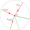
(b)

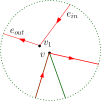
(c)

Figure 10: An illustration of the SOR operation. The edges colored in red depict those edges which have been traversed. It shows the three instance which contribute to the vertex-split. Figure (a) shows the split-pair edges when a vertex $v$ is visited prior to the split corresponding to this split-pair edges. Figure (b) shows the instance when the vertex is revisited through the edge $e_{cycle}$. Figure (c) shows the vertex-split leading to the introduction of the split-vertex $v_{1}$.

This is illustrated in the Figure 10. On every successive revisits to $v$, it is split similarly, and the $i^{th}$ revisit will produce a replica which is labeled as $l^{i}$. Thus, the degree of $v$ is reduced by two in every revisit. Such a traversal breaks all the cycles while maintaining the connectivity of the graph turning it into a tree. We call this method Split-On-Revisit or SOR and the g-tree obtained is called SCESOR-tree.

The algorithm for the SCESOR $\mathcal{GT}$-enhancement is summarized in the pseudocode given in Algorithm 3. The function vertex-split $v$ mentioned in line 2 of the pseudocode refers to the SOR vertex-split operation explained above.

1:if $v$ is visited earlier then                                                  

2:    vertex-split $v$

3:visit $v$

4:while edge($w,v$) in unvisited adjacent edge-list of $v$ do           

5:    SCESOR($w$)

Algorithm 3 SCESOR($v$)

The SCESOR-tree of the graph in Fig. 9(b) is shown in Fig. 11. The five instances of vertex-splits are circled in pink shade in the figure. For vertex 1, it is split into vertex $1^{1}$ with the split-pair being ((0,1),(1,2)). Similarly, we can observe other split-pairs which are marked red in the figure. The prufer code for the gtree is also given in the bottom of the figure. The the label of all the split-vertices appear in the code. Note that they appear exactly once in the code and this is true for an encoding of a SCESOR-tree.

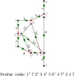
Figure 11: SCESOR-tree of the graph in Fig. 11(b) along with the prufer code.

A SCESOR transformation of a graph $G(E,V)$ splits a subset of vertices in $V$. In the SCESOR-tree thus obtained, the vertices fall into three categories, where a vertex is given a denotation reflecting its category. A vertex $\in V$ that is split, leading to its degree being decremented, is denoted as s-vertex. A vertex belonging to the set of remaining vertices $\in V$, which are not split, is denoted as g-vertex. A replica vertex created by vertex-split is denoted as r-vertex. We make the following observations about a SCESOR-tree. (i) An r-vertex is of degree two, (ii) An s-vertex may be of degree one or more. (iii) If an s-vertex is pendant then its degree in $G$ is odd.

So, only the r-vertices carry the new labels. From the first observation, we conclude that the new labels always appear in the Prüfer code of the SCESOR-tree for any given graph. Hence, the Prüfer code alone is enough to infer the labels of the vertices following the method described in Section III-B, thus decoding the tree.

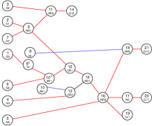
Prüfer code:

$8^{1}$ 9 11 13 16 10 9 18 $10^{1}$ 13 12 15 11 9 12 15 16 16 17 16 18

(a) Tree-partition based method

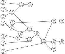
Prüfer code:

$8^{1}$ 9 11 13 16 $10^{1}$ 9 18 $10^{1}$ 13 12 15 11 9 12 15 16 16 17 16 18

(b) SCESOR-based method

Figure 12: An example of g-tree and Prüfer code of s27 using both the methods

The g-trees and the corresponding Prüfer sequences for s27 obtained using the two approaches is given in Figure 12. The two new replica vertices added are $8^{1}$ and $10^{1}$. Figure 12(a) shows the g-tree for the tree-partition-based method. There are two be-trees, marked in blue. The new vertices are pendant and so the vertex-label is swapped for both of them, making the list of extra vertices $L$ empty. However this is not the case with most of the benchmark circuits as depicted in Table I. The SCESOR-tree for s27 is given in Figure 12(b). It can be seen that both the r-vertices are of degree two. As discussed, this method implicitly produces r-vertices of degree two for any given circuit-graph.

In the next section, we will discuss some methods that improve the interpretability of a code by exploring some attributes of a Prüfer code.

VI Prüfer Code Selection

We have seen that the structure of a tree can be fully preserved by its Prüfer code. Besides this primary utility of Prufer codes, another peculiarity about the Prüfer encoding is that the Prufer code for a tree is not unique; a tree can be encoded into a set of distinct Prüfer codes. So this property offers the opportunity to make a choice of a suitable code to represent a g-tree such that the chosen code have the desired requirements. (i) It can be chosen such that it exhibits good interpretability which is an important condition for it be be applicable for ML prupose. (ii) It can also be used so as to preserve the attributes of the graph such as the directions of edges, and (iii) Lastly, it could offer more flexibility such it facilitates learnability of the code. Here, we present three different Prufer codes for g-tree. Before that, we discuss some properties of Prufer encodes to understand how it lends such variety of codes for a tree. Lastly, we discuss about the learnability of such codes.

VI-A Properties of Prüfer Code

Consider an unlabelled tree $T$ with $n$ vertices. A Prüfer code of $T$ has the following properties:

1. A Prüfer encoding induces an edge sequence.

   A Prüfer encoder monitors the list of pendant vertices. Let us call this list Pen_List. In each iteration, Pen_List is updated. From Procedure 1, we recall that the basic operation in each iteration of encoding (decoding) $T$ into a Prüfer sequence is: “choose the pendant vertex ($u$) with the smallest label, encode the label $l_{v}$ of its adjacent vertex ($v$) as the next element of the code, and remove the vertex $u$ from Pen_List. If $v$ is now a pendant vertex, add it to Pen_List”. Thus, in each iteration, an edge ($u,v$) is encoded. Although Prüfer code comprises a string of vertex labels, each label $l_{v}$ in the code actually represents an edge ($u,v$). Hence, a Prüfer code represents a sequence of edges rather than vertices. Out of the set, Edge_Seq, of all possible edge-sequences in a tree, a Prüfer encoding induces a sub-set, Edge_Seq_Prüfer, of the set of edge-sequences. we next look at this sub-set, Edge_Seq_Prüfer.

   For an edge to be selected in a particular iteration, one of its end-vertices should satisfy two conditions:

   1. it should belong to Pen_List, and

   2. it should have the smallest label among them.

   Hence, in order to obtain a desired edge sequence, we need to take care of the above two conditions. The first condition is mostly affected by the structure of tree and hence, we have little control over it. However, the second condition depends on the labeling of vertices. Edge_Seq_Prüfer is the subset of Edge_Seq, where an edge is prioritized on the basis of creating a pendant vertex. An example to demonstrate this is given in Table II. Edges $e_{1}$ and $e_{3}$ of the tree can be named interchangeably because of the symmetry of the tree structure. Note that, the size of the set Edge_Seq is three, and its elements are listed in the first column; first two sequences can be encoded with Prüfer code and so belong to Edge_Seq_Prüfer. The third sequence cannot be encoded by a Prüfer code.

   TABLE II: Edge sequence example.

   Edge-Sequence	Vertex labelling	Prüfer code
   $e_{1}-e_{2}-e_{3}$		2 3
   $e_{1}-e_{3}-e_{2}$		3 4
   $e_{2}-e_{1}-e_{3}$	does not exists	Not possible

2. The vertex-labels of $T$ determine the nature of the Prüfer code.

   This is an important property and follows from the above discussion of Property 1.

3. $T$ can be encoded to a set, $S_{T}$, of distinct Prüfer codes.

   From Property 2, every relabeling of $T$ furnishes a Prüfer code unique to that labeling. Thus, given an unlabeled $T$, it can be represented by several Prüfer codes that make up the set $S_{T}$. The number of such codes is determined by the number of unique labeling of the vertices of $T$.

4. Every Prüfer code in $S_{T}$ decodes to the tree structure of $T$.

   On applying the decoding algorithm on a Prüfer code in $S_{T}$, the structure of $T$ is reconstructed.

5. Prüfer sequences induce a partition on the set $S$, which is the set of Prüfer codes of all possible labeled trees with $n$ vertices such that each partition represents a specific tree structure.

   The Cayley’s formula, $n^{n-2}$, gives the number of labeled trees with $n$ vertices [25]. Prüfer codes provide a bijective proof of Cayley’s formula and so the size of $|S|$ is exactly equal to the number of labeled trees with $n$ vertices. For a given $n$, the number of unlabeled trees is less than the size of $S$ because there exist several labeled trees for a given unlabeled tree. From Property 3, each unlabeled tree $T$, of size $n$ can be represented by a Prüfer code in $S_{T}$. Also, from Property 4, each of them uniquely reconstructs the original tree $T$. Hence, they are mutually exclusive. Furthermore, since every Prüfer code among the $n^{n-2}$ codes reconstructs to some tree of size $n$. The union of the sets $S_{T}$ for all unlabeled trees is thus collectively exhaustive. Therefore, they induce a partition.

VI-B Encoding Methods

From Property 3 and Property 4 it is clear that we can select any code from the partition $S_{T}$ (Property 5) to represent the structure of a gtree, $T_{g}$. Here we present three codes that are generated based on graph relabeling, label reordering, and tree relabeling.

1. Direction-centric code (DCC). For directed acyclic graphs (DAG), a topological ordering of vertices preserves the direction of the edges. So, in this method, the vertices of a graph are labeled in a topological order. Each pair of vertices $(v_{1},v_{2})$, with the edge directed from $v_{1}$ to $v_{2}$, is labeled such that label of $v_{1}$ is smaller than that of $v_{2}$. Since combinatorial logic networks are represented as DAGs, DCC completely preserves the structure of logic networks.

2. Path-centric code (PCC).

   

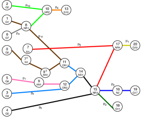
   (a) Path partitions of the graph for circuit s27.

   

   (b) Sequence of single pendant vertices derived from the above code

   

   (c) Prüfer code

   Figure 13: Example of PCC for g-tree of s27.

   In PCC, the labeling scheme is same as DCC, so it preserves the direction of the edges. While in DCC, the edges are not directly interpretable, in PCC, we make the edges interpretable by introducing a change in the ordering of vertices keeping their labels intact. Up till now we have considered that the vertex-labels also determine their ordering, smaller label meaning higher order. In case of PCC, we introcduce a smal change in the ordering for for the leaf nodes of $T_{g}$. Let the set of leaf nodes of $T_{g}$ be $V^{T}_{leaf}$. Here, we assume that the order of vertices in $V^{T}_{leaf}$ is higher than those of non-leaf vertices ($V^{T}\setminus V^{T}_{leaf}$). When this condition in ordering is introduced, the vertices in the set $V^{T}\setminus V^{T}_{leaf}$ that appear in Pen_List are processed before those in $V^{T}_{leaf}$ during encoding/decoding (Refer Section VI-A under Property 1). This has the following implication: For a leaf vertex $u_{leaf}$ of $T_{g}$ we define two terms: (i) junction point ($u_{m}$), the first vertex, of degree greater than two, reachable from $u_{leaf}$, (ii) path-vertices, the set of two-degree vertices that lie between $u_{leaf}$ and its junction point. In the Prüfer code, the path-vertices appear consecutively, in the same sequence as in the path, $u_{leaf}\mathrel{\text{\char 59\relax}}u_{m}$, followed by the junction vertex $u_{m}$. Thus, each of the leaf node, except the last one, induces a path. Also, the order of paths follows that of the corresponding leaf-nodes.

   The edges can be easily reconstructed from their labels if we mark the vertices corresponding to the junction points. They can be marked by traversing the code from right-to-left, and marking those vertex labels which have already appeared (Observation 2).

   An example of PCC for circuit s27 is given in Figure 13. The tree along with eleven paths is shown in Figure 13(a). Note that the vertices in $V^{T}_{leaf}$ are considered in reverse order; higher label means higher order (Figure 13(b)). The Prüfer code with marked junction points is shown in Figure 13(c). For example, the leaf-node 3 induces Path $p_{9}$, whose path-vertices {12,14} and vertex at junction point, vertex labeled 11 appear sequentially in the code.

3. Leaf-centric code (LCC). Although the edges can be reconstructed directly from PCC, the leaf-node needs to be computed beforehand. LCC is a fully edge-interpretable code. The index of a label gives the label of its adjacent vertex. This is possible because each vertex-label in the code represents an edge (Property 1). This is accomplished by complete relabeling of $T_{g}$, denoted by $T_{lcc}^{1}$, which is done as follows: The nodes are partitioned into sets called leaf-stage. The leaves of $T_{g}$ are assigned to the set representing the first stage, $LS1$. Next, on removing the nodes in leaf-stage-1, the leaves of the new tree $T_{lcc}^{2}$ are assigned to $LS2$. Iteratively, the partitions are formed until the entire tree is processed. The final leaf-stage, $LSk$, consists of either a node or a pair of nodes, and is called the tree center [26]. The labeling is done iteratively as follows. Vertices of $LS1$ are labeled from 1 to $|LS1|$. Iteratively, the vertices in $k^{th}$ set is labeled $\sum^{k}_{1}|LS(i-1)|+1$ to $\sum^{k}_{1}|LSi|$. Consider a set $REP\subset V^{T}$, where the vertices in $REP$ were formed by splitting a particular vertex in $G$. Let their labels be $l_{1}\cdots l_{m}$. Let $v\in REP$ have the smallest label ($l_{m}^{\prime}$). For each vertex $u$ in $REP$, with label $l_{u}$, their label is modified as $l_{u}^{l_{m}^{\prime}}$. The additional index is used to store the replica information and does not affect the ordering of vertices while encoding. Such labeling strategy will enforce the label and its index to preserve an edge. Also, the edges belonging to a leaf-stage appear consecutively in LCC.

   There are scope for further improving the interpretability of LCC by adjusting the labels within each leaf-stage. The labels in a leaf-stage subsequence can be made to appear in an ascending order. Considering the tree to be rooted at its center, the vertices can be assigned to different levels progressively. The labeling starts from the vertex (vertices) in the root (level 0). The first vertex is labeled $n$ and subsequent labeling is processed in a decremental order. The labeling is done while moving from lower-level to higher-level nodes, while prioritizing them based on the leaf-stage (higher leaf-stage first). The vertices within a level and belonging to the same leaf-stage are prioritized based on the label of their parents (vertex with higher-labeled parent first).

   Lastly, the direction of the edges can be encoded by marking the labels which represent the edges that are directed one way (converging or diverging) and leaving the edges in the opposite direction unmarked. Thus, besides DAG any directed graph can also be encoded.

   

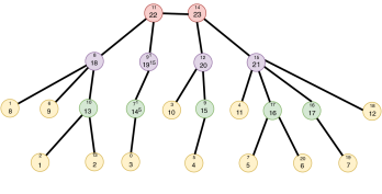
   (a) Relabeled tree of s27 for LCC. The original label is shown in small font. Leaf-stage of vertices is color coded. Vertices with the same level appear horizontally.

   

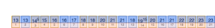
   (b) LCC and the index

   Figure 14: Example of LCC for g-tree of s27.

An example of LCC for s27 is given in Figure 14. Figure 14(a) shows the tree where the root is the edge with vertices marked in red. The new labels are shown in the Figure 14(a). Also, the labeling of vertices within each stage is taken care of so as to improve interpretability. This is reflected in the LCC given in Figure 14(b). Here, the label of the vertex with the corresponding edge incident on it, is marked in orange and one with corresponding edge divergent from it is marked in blue.

VI-C Learnable Representation

Data samples are commonly represented as vectors not only in statistical inference but also in ML, where they are called feature vector. Image data can be viewed as vectors since they are regularly structured on a rectangular lattice. Such representation offers computational ease and lends strong mathematical foundation [3] where huge repository of operations have been defined for vectors. Thus, there are numerous algorithms available that can be used for analyzing vector data in ML. Graphs, however, comprise highly unstructured data and hence cannot naturally be represented as vectors. Although an adjacency matrix can be viewed as structured data, it has several issues which render it difficult to be used as feature vectors. Firstly, for large graphs, the size ($|V|^{2}$) is too large for implementation. Secondly, in scenarios such as graph classification where a single graph is a data sample, it required that the graphs be of similar size. Lastly, even if they are of same size, we need a method to order the nodes so as to induce some correspondence among the nodes of different sample graphs.

Graph embedding has presently emerged as a common solution to above mentioned problems. It captures a certain properties of the graph in the form of vectors. There are of two kinds: (i) node embedding, where each node is represented by a vector. They are used mostly for node classification and link prediction of a graph. They are mostly dependent on the neighborhood information and first/second degree proximity. Some of the examples are Node2Vec [6], LINE [7], DeepWalk [27]; (ii) whole graph embedding. Here the entire graph is represented by a vector which captures some of its properties. They are mostly applicable for graph classification. Such related work includes graph kernels [28] and Subgraph2Vec [29].

Since the aim of our representation is to capture the structural properties of the entire circuit-graph, it needs whole-graph type embedding. However, the existing methods capture only abstracted properties of graph. For example, graphlet-based kernels represent the counts of different kinds of graphlets as a vector. More than just graph classification, we aim to learn structural features from the graph. The proposed Prüfer code captures the structure of the entire graph, and it can handle the scalability issue mentioned earlier. However, the other two issues need to be addressed to make it suitable for graph embedding. The second issue can be handled if the assumption on the size of the graphs (the number of edges in this case), holds, i.e., they are of same order. For graphs representing logical circuits, we can synthesize similar-sized circuits to form the training data. Any difference in their sizes can be handled augmenting them with pseudo-vertices/edges as in [9]. For node correspondence, ordering of the nodes can be accomplished using some special properties [9] such as node-degree. In case of circuit-graphs, some circuit properties such the level of a logic gate in the circuit can also be used.

Once we obtain an ordering of the vertices of the graph $G(V,E)$, we can follow this ordering while traversing the graph during SCESOR traversal. This will enhance th possibility of obtaining a gtree thus will be a unique tree of the graph based on vertex ordering. We can incorporate such ordering to the encoding schemes dicussed in the previous section. Since the topological ordering of a DAG is not unique, in the case of DCC or PCC, the vertices that have the same level are not ordered. So, in such vertices in the graph can be labeled following the ordering of nodes. Also, in the case of LCC, those vertices, which belong to the same tree-level, leaf-stage, or have the same parent are not ordered. So, these additional ordering properties can be applied here also.

VII Conclusion and Future Work

In this work, we have demonstrated a proof-of-concept for lossless and compact encoding of large graphs using just a linear-size sequence of vertex labels. In order to encode graphs with Prüfer codes, we have proposed a method called $\mathcal{GT}$-enhancement, to represent a graph by a tree. We have proposed two techniques for $\mathcal{GT}$-enhancement, and the second technique called SCESOR, allows such tree to be represented by a single code. The focus of the encoding is to capture the structural property of a graph representing a digital circuit, which is essentially a DAG. Among various graph-representation methods used for machine-learning framework, a major issue is to ensure lossless encoding of the structure of the graph. The method based on Prüfer codes completely overcomes this issue. Moreover, we have proposed a labeling technique that preserves the direction of the edges and improves their interpretability. We have discussed the learnability of the code and how they can be used for graph embedding. In general, a learnable representation of the code can potentially be applied for geometric deep learning. Additionally Prüfer code offers a 1-D representation of the graph, which is often a requirement for geometric deep learning [5]. Besides, in the case of g-trees generated from graphs with ordered vertices, the interpretable codes such as LCC bring certain structuredness in the representation, which is required for such applications. Use of such codes in deep learning framework like RNN or CNN can be explored in the future.

References

- [1] I. Chami, S. Abu-El-Haija, B. Perozzi, C. Ré, and K. Murphy, “Machine learning on graphs: A model and comprehensive taxonomy,” 2020.
- [2] H. Cai, V. W. Zheng, and K. C. Chang, “A comprehensive survey of graph embedding: Problems, techniques, and applications,” IEEE Transactions on Knowledge and Data Engineering, vol. 30, no. 9, pp. 1616–1637, Sept 2018.
- [3] Y. Fu and Y. Ma, Graph Embedding for Pattern Analysis. New York: Springer Publishing Company, Incorporated, 2012.
- [4] W. L. Hamilton, R. Ying, and J. Leskovec, “Representation learning on graphs: Methods and applications,” CoRR, vol. abs/1709.05584, 2017.
- [5] M. M. Bronstein, J. Bruna, Y. LeCun, A. Szlam, and P. Vandergheynst, “Geometric deep learning: Going beyond Euclidean data,” IEEE Signal Processing Magazine, vol. 34, no. 4, pp. 18–42, July 2017.
- [6] A. Grover and J. Leskovec, “Node2vec: Scalable feature learning for networks,” in Proc. KDD. ACM, 2016, pp. 855–864.
- [7] J. Tang, M. Qu, M. Wang, M. Zhang, J. Yan, and Q. Mei, “LINE: large-scale information network embedding,” CoRR, vol. abs/1503.03578, 2015.
- [8] M. Defferrard, X. Bresson, and P. Vandergheynst, “Convolutional neural networks on graphs with fast localized spectral filtering,” in Proc. NIPS. Curran Associates, Inc., 2016, pp. 3844–3852.
- [9] M. Niepert, M. Ahmed, and K. Kutzkov, “Learning convolutional neural networks for graphs,” in Proc. ICML, 2016, pp. 2014–2023.
- [10] F. Scarselli, M. Gori, A. C. Tsoi, M. Hagenbuchner, and G. Monfardini, “The graph neural network model,” IEEE Trans. NN, vol. 20, no. 1, pp. 61–80, Jan 2009.
- [11] G. Wang, “A novel neural network model specified for representing logical relations,” CoRR, vol. abs/1708.00580, 2017.
- [12] W. Haaswijk, E. Collins, B. Seguin, M. Soeken, F. Kaplan, S. Süsstrunk, and G. D. Micheli, “Deep learning for logic optimization algorithms,” in Proc ISCAS, 2018, pp. 1–4.
- [13] Y. Dai and R. K. Braytont, “Circuit recognition with deep learning,” in Proc. HOST, 2017, pp. 162–162.
- [14] Y. Ma, H. Ren, B. Khailany, H. Sikka, L. Luo, K. Natarajan, and B. Yu, “High performance graph convolutional networks with applications in testability analysis,” in Proc. DAC, Jun 2019, pp. 1–6.
- [15] M. Pradhan and B. B. Bhattacharya, “A survey of digital circuit testing in the light of machine learning,” WIREs Data Mining and Knowledge Discovery, p. e1360, 2020.
- [16] M. Pradhan, B. B. Bhattacharya, K. Chakrabarty, and B. B. Bhattacharya, “Predicting -sensitivity of circuit-inputs on test-coverage: A machine-learning approach,” Proc. TCAD, vol. 38, no. 12, pp. 2343–2356, 2019.
- [17] H. Prufer, “Neuer beweis eines satzes uber permutationen,” Arch. Math. Phys., vol. 27, pp. 742–744, 1918.
- [18] F. Brglez, D. Bryan, and K. Kozminski, “Combinational profiles of sequential benchmark circuits,” in Proc. ISCAS, 1989, pp. 1929–1934.
- [19] F. Corno, M. Reorda, and G. Squillero, “RT-level ITC’99 benchmarks and first ATPG results,” IEEE Design and Test of Computers, vol. 17, no. 3, pp. 44–53, Jul 2000.
- [20] T. Biedl and F. J. Brandenburg, “Partitions of graphs into trees,” in Proc. Graph Drawing, 2007, pp. 430–439.
- [21] J. Gottlieb, B. A. Julstrom, G. R. Raidl, and F. Rothlauf, “Prüfer numbers: A poor representation of spanning trees for evolutionary search,” in Proc. GECCO, 2001, pp. 343–350.
- [22] X. Wang, L. Wang, and Y. Wu, “An optimal algorithm for prufer codes,” JSEA, vol. 2, pp. 111–115, 01 2009.
- [23] T. H. Cormen, C. Stein, R. L. Rivest, and C. E. Leiserson, Introduction to Algorithms, 2nd ed. Cambridge: McGraw-Hill Higher Education, 2001.
- [24] A. B. Kahn, “Topological sorting of large networks,” Commun. ACM, vol. 5, no. 11, pp. 558–562, Nov. 1962.
- [25] P. W. Shor, “A new proof of cayley’s formula for counting labeled trees,” Journal of Combinatorial Theory, Series A, vol. 71, no. 1, pp. 154 – 158, 1995.
- [26] F. Harary, Graph Theory, ser. Addison Wesley Series in Mathematics. Boston: Addison-Wesley, 1971.
- [27] B. Perozzi, R. Al-Rfou, and S. Skiena, “Deepwalk: Online learning of social representations,” in Proc. KDD. ACM, 2014, pp. 701–710.
- [28] P. Yanardag and S. Vishwanathan, “Deep graph kernels,” in Proc. ACM SIGKDD. New York, NY, USA: ACM, 2015, pp. 1365–1374.
- [29] A. Narayanan, M. Chandramohan, L. Chen, Y. Liu, and S. Saminathan, “subgraph2vec: Learning distributed representations of rooted sub-graphs from large graphs,” CoRR, vol. abs/1606.08928, 2016.