Big Bang Nucleosynthesis constraints on $f(T,T_{G})$ gravity

Abstract

We confront $f(T,T_{G})$ gravity, with Big Bang Nucleosynthesis (BBN) requirements. The former is obtained using both the torsion scalar, as well as the teleparallel equivalent of the Gauss-Bonnet term, in the Lagrangian, resulting to modified Friedmann equations in which the extra torsional terms constitute an effective dark energy sector. We calculate the deviations of the freeze-out temperature $T_{f}$, caused by the extra torsion terms in comparison to $\Lambda$CDM paradigm. Then we impose five specific $f(T,T_{G})$ models and we extract the constraints on the model parameters in order for the ratio $|\Delta T_{f}/T_{f}|$ to satisfy the observational BBN bound. As we find, in most of the models the involved parameters are bounded in a narrow window around their General Relativity values as expected, as in the power-law model where the exponent $n$ needs to be $n\lesssim 0.5$. Nevertheless the logarithmic model can easily satisfy the BBN constraints for large regions of the model parameters. This feature should be taken into account in future model building.

I Introduction

There are two motivations that lead to the construction of modifications of gravity. The first is purely theoretical, namely to construct gravitational theories that do not suffer from the renormalizability problems of general relativity and thus being closer to a quantum description Stelle:1976gc ; Addazi:2021xuf . The second is cosmological, namely to construct gravitational theories that at a cosmological framework can describe the early and late accelarating eras Nojiri:2010wj ; Clifton:2011jh ; Nojiri:2017ncd ; CANTATA:2021ktz ; Ishak:2018his , as well as to alleviate various observational tensions Abdalla:2022yfr .

There is a rich literature on modified and extended theories of gravity. One may start from the Einstein-Hilbert Lagrangian and add extra terms, resulting in $f(R)$ gravity Starobinsky:1980te ; Capozziello:2002rd ; DeFelice:2010aj , in $f(G)$ gravity Antoniadis:1993jc ; Nojiri:2005jg ; DeFelice:2008wz , in $f(G,{\cal{T}})$ theories Yousaf:2021xex , in $f(P)$ gravity Erices:2019mkd ; Marciu:2020ysf ; Jimenez:2020gbw in Lovelock gravity Lovelock:1971yv ; Deruelle:1989fj , in Weyl gravity Mannheim:1988dj , in Horndeski/Galileon scalar-tensor theories Horndeski:1974wa ; Deffayet:2009wt etc. Nevertheless, one can follow a different approach, and add new terms to the equivalent torsional formulation of gravity, resulting to $f(T)$ gravity Bengochea:2008gz ; Cai:2015emx , to $f(T,T_{G})$ gravity Kofinas:2014owa ; Kofinas:2014aka ; Kofinas:2014daa , to $f(T,B)$ gravity Bahamonde:2015zma ; Bahamonde:2016grb , to scalar-torsion theories Geng:2011aj etc. Torsional gravity has been proven to exhibit interesting phenomenology, both at the cosmological framework Chen:2010va ; Wu:2010mn ; Dent:2010nbw ; Myrzakulov:2010vz ; Zheng:2010am ; Tamanini:2012hg ; Bamba:2012vg ; Dong:2012en ; Karami:2012fu ; Liu:2012fk ; Otalora:2013tba ; Ong:2013qja ; Chen:2014qtl ; Farrugia:2016qqe ; Bejarano:2017akj ; Hohmann:2017jao ; Bahamonde:2017wwk ; Abedi:2018lkr ; Golovnev:2018wbh ; Krssak:2018ywd ; Deng:2018ncg ; Cai:2019bdh ; Caruana:2020szx ; Ren:2021tfi ; Briffa:2021nxg ; Benisty:2021sul ; Dialektopoulos:2021ryi ; Papagiannopoulos:2022ohv ; Papanikolaou:2022hkg , as well as at the level of local, spherically symmetric solutions Wang:2011xf ; Boehmer:2011gw ; Ferraro:2011ks ; Meng:2011ne ; Rodrigues:2012qua ; Rodrigues:2013ifa ; Nashed:2013bfa ; Bejarano:2014bca ; Das:2015gwa ; Mai:2017riq ; Mustafa:2019eet ; Nashed:2020kjh ; Pfeifer:2021njm ; Ren:2021uqb ; Bahamonde:2021srr ; Bahamonde:2022lvh ; Huang:2022slc ; Zhao:2022gxl .

One crucial test that every modification of gravity should pass, that is usually underestimated in the literature, is the confrontation with the Big Bang Nucleosynthesis (BBN) dataBernstein:1988ad ; Kolb:1990vq ; Olive:1999ij ; Cyburt:2015mya ; Asimakis:2021yct . Specifically, the amount of modification needed in order to fulfill the late-time cosmological requirements must not at the same time spoil the successes of early-time cosmology, and among them the BBN phase. Hence, whatever are the advantages of a specific modified theory of gravity, if it cannot satisfy the BBN constraints it must be excluded Torres:1997sn ; Lambiase:2005kb ; Lambiase:2011zz ; Anagnostopoulos:2022gej .

In the present manuscript we are interested in investigating the BBN epoch in a universe governed by $f(T,T_{G})$ gravity. In particular, we desire to study various specific models that are known to lead to viable phenomenology, and extract constrains on the involved model parameters. The plan of the article is the following: In Section II we briefly present $f(T,T_{G})$ gravity, extracting the field equations and applying them to a cosmological framework. In Section III we summarize the BBN formalism and we provide the difference in the freeze-out temperature caused by the extra torsion terms. Then in Section IV we investigate five specific $f(T,T_{G})$ models, confronting them with the observational BBN bounds. Finally, Section V is devoted to the Conclusions.

II $f(T,T_{G})$ gravity

In this section we briefly review $f(T,T_{G})$ gravity Kofinas:2014owa ; Kofinas:2014aka ; Kofinas:2014daa . As usual in torsional formulation of gravity we use the tetrad field as the dynamical variable, which forms an orthonormal basis at the tangent space. In a coordinate basis one can relate it with the metric through $g_{\mu\nu}(x)=\eta_{AB}e^{A}_{\mu}(x)e^{B}_{\nu}(x)$, where $\eta_{AB}=\text{diag}(-1,1,1,1)$, and with Greek and Latin letters denoting coordinate and tangent indices respectively. Applying the Weitzenböck connection ${W}^{\lambda}_{\nu\mu}\equiv e^{\lambda}_{A}\>\partial_{\mu}e^{A}_{\nu}$ Cai:2015emx , the corresponding torsion tensor is

$${T}^{\lambda}_{\>\mu\nu}\equiv{W}^{\lambda}_{\nu\mu}-{W}^{\lambda}_{\mu\nu}=e^{\lambda}_{A}\>(\partial_{\mu}e^{A}_{\nu}-\partial_{\nu}e^{A}_{\mu})~{},$$ (1)

and then the torsion scalar is obtained through the contractions

$$T\equiv\frac{1}{4}T^{\rho\mu\nu}T_{\rho\mu\nu}+\frac{1}{2}T^{\rho\mu\nu}T_{\nu\mu\rho}-T_{\rho\mu}^{\ \ \rho}T_{\ \ \ \nu}^{\nu\mu}~{},$$ (2)

and incorporates all information of the gravitational field. Used as a Lagrangian, the torsion scalar gives rise to exactly the same equations with General Relativity, that is why the theory was named teleparallel equivalent of general relativity (TEGR).

Similarly to curvature gravity, where one can construct higher-order invariants such as the Gauss-Bonnet one, in torsional gravity one may construct higher-order torsional invariants, too. In particular, since the curvature (Ricci) scalar and the torsion scalar differ by a total derivative, in Kofinas:2014owa the authors followed the same recipe and extracted a higher-order torsional invariant which differs from the Gauss-Bonnet one by a boundary term, namely

$$\!\!\!\!\!\!\!\!\!\!\!\!\!\!T_{G}=\left(K^{\kappa}_{\,\,\,\varphi\pi}K^{\varphi\lambda}_{\,\,\,\,\,\,\,\rho}K^{\mu}_{\,\,\,\,\chi\sigma}K^{\chi\nu}_{\,\,\,\,\,\,\,\tau}-2K^{\kappa\!\lambda}_{\,\,\,\,\,\,\pi}K^{\mu}_{\,\,\,\varphi\rho}K^{\varphi}_{\,\,\,\chi\sigma}K^{\chi\nu}_{\,\,\,\,\,\,\tau}\right.$$

$$\!\!\!\!\!\!\!\!\!\!\!\!\!\!\left.+2K^{\kappa\!\lambda}_{\,\,\,\,\,\,\pi}K^{\mu}_{\,\,\,\,\varphi\rho}K^{\varphi\nu}_{\,\,\,\,\,\,\chi}K^{\chi}_{\,\,\,\,\sigma\tau}+2K^{\kappa\!\lambda}_{\,\,\,\,\,\,\pi}K^{\mu}_{\,\,\,\,\varphi\rho}K^{\varphi\nu}_{\,\,\,\,\,\,\,\sigma,\tau}\right)\delta^{\pi\rho\sigma\tau}_{\kappa\lambda\mu\nu},$$ (3)

where $K^{\mu\nu}_{\>\>\>\>\rho}\equiv-\frac{1}{2}\Big{(}T^{\mu\nu}_{\>\>\>\>\rho}-T^{\nu\mu}_{\>\>\>\>\rho}-T_{\rho}^{\>\>\>\>\mu\nu}\Big{)}$ is the contortion tensor and the generalized $\delta^{\pi\rho\sigma\tau}_{\kappa\lambda\mu\nu}$ denotes the determinant of the Kronecker deltas. Note that similarly to the Gauss-Bonnet term, the teleparallel equivalent of the Gauss-Bonnet term $T_{G}$ is also a topological invariant in four dimensions.

Using the above torsional invariants one can construct the new class of $f(T,T_{G})$ gravitational modifications, characterized by the action Kofinas:2014owa

$$S=\frac{M_{P}^{2}}{2}\!\int d^{4}x\,e\,f(T,T_{G})\,,$$ (4)

with $M_{P}^{2}$ the reduced Planck mass. The general field equations of the above action can be found in Kofinas:2014owa , where one can clearly see that the theory is different from $f(R)$, $f(R,G)$ and $f(T)$ gravitational modifications, and thus it corresponds to a novel class of modified gravity.

In this work we are interested in the cosmological applications of $f(T,T_{G})$ gravity. Hence, we consider a spatially flat Friedmann-Robertson-Walker (FRW) metric of the form

$$ds^{2}=-dt^{2}+a^{2}(t)\delta_{ij}dx^{i}dx^{j}\,,$$ (5)

with $a(t)$ the scale factor, which corresponds to the diagonal tetrad

$$e^{A}_{\,\,\,\mu}=\text{diag}(1,a(t),a(t),a(t)).$$ (6)

In this case, the torsion scalar (2) and the teleparallel equivalent of the Gauss-Bonnet term (3) become

$$T=6H^{2}$$ (7)

$$T_{G}=24H^{2}\big{(}\dot{H}+H^{2}\big{)},$$ (8)

with $H=\frac{\dot{a}}{a}$ the Hubble parameter and where dots denoting derivatives with respect to $t$.

The general field equations for the FRW geometry are Kofinas:2014aka

$$\!\!\!\!\!\!\!\!\!\!\!\!\!\!f-12H^{2}f_{T}-T_{G}f_{T_{G}}+24H^{3}\dot{f_{T_{G}}}=2M_{P}^{-2}(\rho_{r}+\rho_{m})$$ (9)

$$\!\!\!\!\!\!\!\!\!\!\!\!\!\!f-4\big{(}3H^{2}+\dot{H}\big{)}f_{T}-4H\dot{f_{T}}-T_{G}f_{T_{G}}$$

$$\!\!\!\!\!\!\!\!\!+\frac{2}{3H}T_{G}\dot{f_{T_{G}}}+8H^{2}\ddot{f_{T_{G}}}=-2M_{P}^{-2}(p_{r}+p_{m})\,,$$ (10)

with $\dot{f_{T}}=f_{TT}\dot{T}+f_{TT_{G}}\dot{T}_{G}$, $\dot{f_{T_{G}}}=f_{TT_{G}}\dot{T}+f_{T_{G}T_{G}}\dot{T}_{G}$, and $\ddot{f_{T_{G}}}=f_{TTT_{G}}\dot{T}^{2}+2f_{TT_{G}T_{G}}\dot{T}\dot{T}_{G}+f_{T_{G}T_{G}T_{G}}\dot{T}_{G}^{\,\,2}+f_{TT_{G}}\ddot{T}+f_{T_{G}T_{G}}\ddot{T}_{G}$, and where $f_{TT}$, $f_{TT_{G}}$,… denote multiple partial differentiations with respect to $T$ and $T_{G}$. Note that in the above equations we have also introduced the radiation and matter sectors, corresponding to perfect fluids with energy densities $\rho_{r}$,$\rho_{m}$ and pressures $p_{r}$,$p_{m}$, respectively. Lastly, we mention that the above equations for $f(T,T_{G})=-T+\Lambda$ recover the TEGR and General Relativity equations, where $\Lambda$ is the cosmological constant.

As we can see, we can re-write the Friedmann equations (9) and (10) in the usual form

$$\!\!\!\!\!\!\!\!\!\!\!\!3M_{P}^{2}H^{2}=\left(\rho_{r}+\rho_{m}+\rho_{DE}\right)$$ (11)

$$\!\!\!\!\!\!\!\!\!\!\!\!-2M_{P}^{2}\dot{H}=\left(\rho_{r}+p_{r}+\rho_{m}+p_{m}+\rho_{DE}+p_{DE}\right),$$ (12)

where we have defined the effective dark energy density and pressure as

$$\!\!\!\!\!\!\rho_{DE}\equiv\frac{M_{P}^{2}}{2}\!\left(\!6H^{2}\!-\!f\!+\!12H^{2}f_{T}\!+\!T_{G}f_{T_{G}}\!-\!24H^{3}\dot{f_{T_{G}}}\!\right),$$ (13)

$$\!\!\!\!\!\!\!\!\!\!\!\!\!\!\!\!\!\!\!\!\!\!\!\!p_{DE}\equiv\frac{M_{P}^{2}}{2}\left[-2(2\dot{H}+3H^{2})+f-4\big{(}\dot{H}+3H^{2}\big{)}f_{T}\right.$$

$$\left.\!\!\!\!\!-4H\dot{f_{T}}-T_{G}f_{T_{G}}+\frac{2}{3H}T_{G}\dot{f_{T_{G}}}+8H^{2}\ddot{f_{T_{G}}}\right],$$ (14)

of gravitational origin.

III Big Bang Nucleosynthesis constraints

Big Bang Nucleosynthesis (BBN) was a process that took place during radiation era. Let us first present the framework which provides the BBN constraints through standard cosmology Bernstein:1988ad ; Kolb:1990vq ; Olive:1999ij ; Cyburt:2015mya ; Asimakis:2021yct . The first Friedmann equation from Einstein-Hilbert action can be written as

$$3H^{2}=M_{P}^{-2}\rho,$$ (15)

where $\rho=\rho_{r}+\rho_{m}$. In the radiation era the radiation sector dominates hence we can write

$$H^{2}\approx\frac{M_{P}^{-2}}{3}\rho_{r}\equiv H_{GR}^{2}.$$ (16)

In addition it is known that the energy density of relativistic particles is

$${\displaystyle\rho_{r}=\frac{\pi^{2}}{30}g_{*}{T}^{4}},$$ (17)

where $g_{*}\sim 10$ the effective number of degrees of freedom and ${T}$ the temperature. Thus , if we combine (16) with (17) we obtain

$$H(T)\approx\left(\frac{4\pi^{3}g_{*}}{45}\right)^{1/2}\frac{{T}^{2}}{M_{Pl}},$$ (18)

where $M_{Pl}=(8\pi)^{\frac{1}{2}}M_{P}=1.22\times 10^{19}$ GeV is the Planck mass.

During the radiation era the scale factor evolves as $a(t)\sim t^{1/2}$. Therefore, using the relation of Hubble parameter with scale factor we find that in the radiation era the Hubble parameter evolves as $H(t)=\frac{1}{2t}$. Combining the last one with (18) we find the relation between temperature and time. Thus, we have ${\displaystyle\frac{1}{t}\simeq\left(\frac{32\pi^{3}g_{*}}{90}\right)^{1/2}\frac{{T}^{2}}{M_{Pl}}}$ (or ${T}(t)\simeq(t/\text{sec})^{-1/2}$ MeV).

During the BBN we have interactions between particles. For example we have interactions between neutrons, protons, electrons and neutrinos, namely $n+\nu_{e}\to p+e^{-}$, $n+e^{+}\to p+{\bar{\nu}}_{e}$ and $n\to p+e^{-}+{\bar{\nu}}_{e}$. We name the conversion rate from a particle A to particle B as $\lambda_{BA}$. Hence, the conversion rate from neutrons to protons is $\lambda_{pn}$ and it is equal to the sum of the three interaction conversion rates written above. Therefore, the calculation of the neutron abundance arises from the protons-neutron conversion rate Olive:1999ij ; Cyburt:2015mya

$$\lambda_{pn}({T})=\lambda_{(n+\nu_{e}\to p+e^{-})}+\lambda_{(n+e^{+}\to p+{\bar{\nu}}_{e})}+\lambda_{(n\to p+e^{-}+{\bar{\nu}}_{e})}\,$$ (19)

and its inverse $\lambda_{np}({T})$, and therefore for the total rate we have $\lambda_{tot}({T})=\lambda_{np}({T})+\lambda_{pn}({T})$. Now, we assume that the various particles (neutrinos, electrons, photons) temperatures are the same, and low enough in order to use the Boltzmann distribution instead of the Fermi-Dirac one, and we neglect the electron mass compared to the electron and neutrino energies. The final expression for the conversion rate is Torres:1997sn ; Lambiase:2005kb ; Lambiase:2011zz ; Anagnostopoulos:2022gej

$$\lambda_{tot}({T})=4A\,{T}^{3}(4!{T}^{2}+2\times 3!{Q}{T}+2!{Q}^{2})\,,$$ (20)

where ${Q}=m_{n}-m_{p}=1.29\times 10^{-3}$GeV is the mass difference between neutron and proton and $A=1.02\times 10^{-11}$ GeV^-4.

We proceed in calculating the corresponding freeze-out temperature. This will arise comparing the universe expansion rate $\frac{1}{H}$ with $\lambda_{tot}\left(T\right)$. In particular, if $\frac{1}{H}\ll\lambda_{tot}\left(T\right)$, namely if the expansion time is much smaller than the interaction time, we can consider thermal equilibrium Bernstein:1988ad ; Kolb:1990vq . On the contrary, if $\frac{1}{H}\gg\lambda_{tot}\left(T\right)$ then particles do not have enough time to interact so they decouple. The freeze-out temperature $T_{f}$, in which the decoupling takes place, corresponds to $H(T_{f})=\lambda_{tot}\left(T_{f}\right)\simeq c_{q}\,T_{f}^{5}$, with $c_{q}\equiv 4A\,4!\simeq 9.8\times 10^{-10}\,{\rm GeV}^{-4}$ Torres:1997sn ; Lambiase:2005kb ; Lambiase:2011zz ; Anagnostopoulos:2022gej . Now if we use (18) and $H(T_{f})=\lambda_{tot}\left(T_{f}\right)\simeq c_{q}\,T_{f}^{5}$, we acquire

$$T_{f}=\left(\frac{4\pi^{3}g_{*}}{45M_{Pl}^{2}c_{q}^{2}}\right)^{1/6}\sim 0.0006~{}{\rm GeV}.$$ (21)

Using modified theories we obtain extra terms in energy density due to the modification of gravity. The first Friedmann equation (11) during radiation era becomes

$$3M_{P}^{2}H^{2}=\rho_{r}+\rho_{DE},$$ (22)

where $\rho_{DE}$ must be very small compared to $\rho_{r}$ in order to be in accordance with observations. Hence, we can write (22) using (16) as

$$H=H_{GR}\sqrt{1+\frac{\rho_{DE}}{\rho_{r}}}=H_{GR}+\delta H,$$ (23)

where $H_{GR}$ is the Hubble parameter of standard cosmology. Thus, we have $\Delta H=\left(\sqrt{1+\frac{\rho_{DE}}{\rho_{r}}}-1\right)H_{GR}$, which quantifies the deviation from standard cosmology, i.e form $H_{GR}$. This will lead to a deviation in the freeze-out temperature $\Delta T_{f}$. Since $H_{GR}=\lambda_{tot}\approx c_{q}\,T_{f}^{5}$ and $\sqrt{1+\frac{\rho_{DE}}{\rho_{r}}}\approx 1+\frac{1}{2}\frac{\rho_{DE}}{\rho_{r}}$, we easily find

$$\left(\sqrt{1+\frac{\rho_{DE}}{\rho_{r}}}-1\right)H_{GR}=5c_{q}\,T_{f}^{4}\Delta T_{f},$$ (24)

and finally

$$\frac{\Delta T_{f}}{T_{f}}\simeq\frac{\rho_{DE}}{\rho_{r}}\frac{H_{GR}}{10c_{q}\,T_{f}^{5}},$$ (25)

where we used that $\rho_{DE}<<\rho_{r}$ during BBN era. This theoretically calculated $\frac{\Delta T_{f}}{T_{f}}$ should be compared with the observational bound

$$\left|\frac{\Delta{T}_{f}}{{T}_{f}}\right|<4.7\times 10^{-4}\,,$$ (26)

which is obtained from the observational estimations of the baryon mass fraction converted to ${}^{4}He$ Coc:2003ce ; Olive:1996zu ; Izotov:1998mj ; Fields:1998gv ; Izotov:1999wa ; Kirkman:2003uv ; Izotov:2003xn .

IV BBN constraints on $f(T,T_{G})$ gravity

In this section we will apply the BBN analysis in the case of $f(T,T_{G})$ gravity. Let us mention here that in general, in modified gravity, inflation is not straightaway driven by an inflaton field but the inflaton is hidden inside the gravitational modification, i.e. it is one of the extra scalar degrees of freedom of the modified graviton. Hence, in such frameworks reheating is usually performed gravitationally, and the reheating and BBN temperatures may differ from standard ones. Nevertheless, in the present work we make the assumption that we do not deviate significantly from the successful concordance scenario, in order to examine whether $f(T,T_{G})$  gravity can at first pass BBN constraints or not. Clearly a more general analysis should be performed in a separate project, to cover more radical cases too. In the following, we will examine five specific models that are considered to be viable in the literature.

IV.0.1 Model I: $f=-T+\beta_{1}\sqrt{T^{2}+\beta_{2}T_{G}}$

Firstly we investigate the model $f=-T+\beta_{1}\sqrt{T^{2}+\beta_{2}T_{G}}$ Kofinas:2014daa . Since in our analysis we focus on the radiation era where the Hubble parameter $H(t)=\frac{1}{2t}$, we can express the derivatives of the Hubble parameter as powers of the Hubble parameter itself, e.g. $\dot{H}=-2H^{2}$ and $\ddot{H}=8H^{3}$. Additionally, in order to eliminate one model parameter we will apply the Friedmann equation at present time, requiring

$$\Omega_{DE0}\equiv\rho_{DE0}/(3M_{P}^{2}H_{0}^{2}),$$ (27)

where $\Omega_{DE}$ is the dark energy density parameter and with the subscript “0” denoting the value of a quantity at present time. Doing so, and inserting $f=-T+\beta_{1}\sqrt{T^{2}+\beta_{2}T_{G}}$ into (13) and then into (25), we finally find

$$\!\!\!\!\!\!\!\!\frac{\Delta T_{f}}{T_{f}}=(10c_{q}T_{f}^{3})^{-1}\zeta H_{0}\Omega_{DE0}\left(3-2\beta_{2}\right)^{-3/2}\\ \cdot\left(9-15\beta_{2}+6\beta_{2}^{2}\right)\left[\left(3+2\beta_{2}\right)H_{0}^{2}+2\beta_{2}\dot{H}_{0}\right]^{3/2}\\ \cdot\left[\left(9+3\beta_{2}-2\beta_{2}^{2}\right)H_{0}^{4}+9\beta_{2}H_{0}^{2}\dot{H}_{0}+\beta_{2}^{2}H_{0}\ddot{H}_{0}\right]^{-1},$$ (28)

where

$$\zeta\equiv\left(\frac{4\pi^{3}g_{*}}{45}\right)^{\frac{1}{2}}M_{Pl.}^{-1}~{}.$$ (29)

In this expression we insert Planck

$$\Omega_{DE0}\approx 0.7,\quad H_{0}=1.4\times 10^{-42}~{}{\rm GeV},$$ (30)

and the derivatives of the Hubble function at present are calculated through $\dot{H}_{0}=-H_{0}^{2}\left(1+q_{0}\right)$ and $\ddot{H}_{0}=H_{0}^{3}\left(j_{0}+3q_{0}+2\right)$ with $q_{0}=-0.503$ the current decceleration parameter of the Universe Planck , and $j_{0}=1.011$ the current jerk parameter Visser:2003vq ; Mamon:2018dxf . Hence, $\dot{H}_{0}\approx-9.7\times 10^{-85}\,$GeV² and $\ddot{H}_{0}\approx 4.1\times 10^{-126}\,$GeV³.

Using the BBN constraint (26) we conclude that $\beta_{2}\in\left(-2.98,-2.93\right)$ $\cup$ $\left(0.99,1.01\right)$, where we have used (27) to find

$$\!\!\!\!\!\beta_{1}=\sqrt{3}H_{0}\Omega_{DE0}\left[\left(3+2\beta_{2}\right)H_{0}^{2}+2\beta_{2}\dot{H}_{0}\right]^{3/2}\\ \!\!\cdot\left[\left(9+3\beta_{2}-2\beta_{2}^{2}\right)H_{0}^{4}+9\beta_{2}H_{0}^{2}\dot{H}_{0}+\beta_{2}^{2}H_{0}\ddot{H}_{0}\right]^{-1}.$$ (31)

Using the above range of $\beta_{2}$ we find that $\beta_{1}\in\left(2.09\times 10^{-26},0.001\right)$ $\cup$ $\left(1.380,1.384\right)$.

In Fig. 1 we depict $|\Delta T_{f}/T_{f}|$ appearing in (28) versus the model parameter $\beta_{2}$. As we can see the allowed range is within the vertical dashed lines.

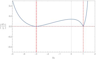
Figure 1: $|\Delta T_{f}/T_{f}|$ vs the model parameter $\beta_{2}$ (blue solid curve), for Model I: $f=-T+\beta_{1}\sqrt{T^{2}+\beta_{2}T_{G}}$. The allowed range of $\beta_{2}$, where (26) is satisfied (horizontal red dashed line), is within the vertical dashed lines.

IV.0.2 Model II: $f=-T+a_{1}T^{2}+a_{2}T\sqrt{|T_{G}|}$

Let us now study the case $f=-T+a_{1}T^{2}+a_{2}T\sqrt{|T_{G}|}$, where $a_{1}$,$a_{2}$ are the free parameters of the theory Kofinas:2014daa . In this case we find

$$\frac{\Delta T_{f}}{T_{f}}=\frac{3}{10}c_{q}^{-1}\zeta^{3}T_{f}\Bigg{\{}\frac{\Omega_{DE0}}{3H_{0}^{2}}\\ -\sqrt{6}a_{2}\Bigg{[}\frac{\sqrt{H_{0}^{2}+\dot{H_{0}}}}{6H_{0}}\Big{(}6-\frac{2\dot{H}_{0}^{2}-H_{0}\ddot{H}_{0}}{H_{0}^{2}+\dot{H}_{0}}\Big{)}-1\Bigg{]}\Bigg{\}}.$$ (32)

Using the constraint (26), ans since according to (32) $\Delta{T}_{f}/{T}_{f}$ is linear in $a_{2}$, we deduce that (32) is valid for a small region around $2.7\times 10^{83}~{}{\rm GeV}^{-2}$, where we have used the constraint from current cosmological era (27)

$$a_{1}=\frac{\Omega_{DE0}}{18H_{0}^{2}}-\sqrt{6}a_{2}\frac{\sqrt{H_{0}^{2}+\dot{H_{0}}}}{36H_{0}}\left[6-\frac{2\dot{H}_{0}^{2}-H_{0}\ddot{H}_{0}}{\left(H_{0}^{2}+\dot{H}_{0}\right)^{2}}\right].$$ (33)

Using the above value of $a_{2}$ we find that $a_{1}=-1.1\times 10^{83}~{}{\rm GeV}^{-2}$.

IV.0.3 Model III: $f\!=\!-T+\beta_{1}\sqrt{T^{2}\!+\!\beta_{2}T_{G}}+a_{1}T^{2}+a_{2}T\sqrt{|T_{G}|}$

Now we analyze the model $f=-T+\beta_{1}\sqrt{T^{2}+\beta_{2}T_{G}}+a_{1}T^{2}+a_{2}T\sqrt{|T_{G}|}$, where we have four free parameters, namely $\beta_{1}$, $\beta_{2}$, $a_{1}$, $a_{2}$ Kofinas:2014daa . In order to simplify the analysis we will impose the constraint $-2.99<\beta_{2}<\frac{3}{2}$, obtained above.

In this case we find

$$\frac{\Delta T_{f}}{T_{f}}=-\left(60c_{q}T_{f}^{3}\right)^{-1}\!\left\{3\sqrt{12}\beta_{1}\left(3\!-\!2\beta_{2}\right)^{-1/2}\left(1\!+\!\beta_{2}\!-\!2\beta_{1}\right)\right.\\ -18\Big{\{}\frac{\Omega_{DE0}}{3H_{0}^{2}}+\frac{\sqrt{12}\beta_{1}}{18H_{0}^{3}}\left[\left(3+2\beta_{2}\right)H_{0}^{2}+2\beta_{2}\dot{H}_{0}\right]^{-1/2}\\ \left.\left.\!\!\!\!\!\!\!\!\!\!\!\!\!\!\!\!\!\!\!\!\!\!\!\!\cdot\left[\left(3\!-\!6\beta_{1}\!+\!2\beta_{2}\right)H_{0}^{2}+2\beta_{2}\dot{H}_{0}\right]\right.\right.\\ \left.\left.\ \ \ \ \ \ \ \ -\frac{a_{2}}{\sqrt{6}H_{0}}\sqrt{H_{0}^{2}+\dot{H}_{0}}\Bigg{[}6-\frac{2\dot{H}_{0}^{2}-H_{0}\ddot{H}_{0}}{(H_{0}^{2}+\dot{H}_{0})^{2}}\Bigg{]}+\sqrt{6}a_{2}\right.\right.\\ \left.\left.-\frac{\sqrt{12}\beta_{1}\beta_{2}}{18H_{0}^{3}}\left[\left(3+2\beta_{2}\right)H_{0}^{2}+2\beta_{2}\dot{H}_{0}\right]^{-3/2}\right.\right.\\ \!\!\!\!\!\!\!\!\cdot\left[\left(3+2\beta_{2}\right)H_{0}^{4}+\left(9+8\beta_{2}\right)H_{0}^{2}\dot{H}_{0}\right.\\ \left.\left.+\beta_{2}\left(4\dot{H}_{0}^{2}+H_{0}\ddot{H}_{0}\right)\right]\Big{\}}\zeta^{2}T_{f}^{4}\right\}\zeta.$$ (34)

Observing that expression (34) is linear in $a_{2}$, and using the constraint (26) and two values for $\beta_{1}$ from the aforementioned range we extracted in model I, i.e. $\beta_{1}=1.4$ and $\beta_{2}=1$, we find that (32) is valid for a small region around the point $-3.5\times 10^{83}~{}{\rm GeV}^{-2}$. Using another set of values ($\beta_{1}=0.001$, $\beta_{2}\approx-2.96$) we find that (32) is valid for a small region around the point $-5.3\times 10^{83}~{}{\rm GeV}^{-2}$, where we have used

$$\!\!\!\!\!\!\!a_{1}=\frac{\Omega_{DE0}}{18H_{0}^{2}}+\frac{\sqrt{12}\beta_{1}}{108H_{0}^{3}}\left[\left(3+2\beta_{2}\right)H_{0}^{2}+2\beta_{2}\dot{H}_{0}\right]^{-1/2}\\ \left[\left(3-6\beta_{1}+2\beta_{2}\right)H_{0}^{2}+2\beta_{2}\dot{H}_{0}\right]\\ -\frac{\sqrt{6}}{36}\frac{a_{2}}{H_{0}}\sqrt{H_{0}^{2}+\dot{H}_{0}}\left(6-\frac{2\dot{H}_{0}^{2}-H_{0}\ddot{H}_{0}}{\left(H_{0}^{2}+\dot{H}_{0}\right)^{2}}\right)\\ -\frac{\sqrt{12}\beta_{1}\beta_{2}}{108H_{0}^{3}}\left[\left(3+2\beta_{2}\right)H_{0}^{2}+2\beta_{2}\dot{H}_{0}\right]^{-3/2}\\ \times\left[\left(3+2\beta_{2}\right)H_{0}^{4}+\left(9+8\beta_{2}\right)H_{0}^{2}\dot{H}_{0}+\beta_{2}\left(4\dot{H}_{0}^{2}+H_{0}\ddot{H}_{0}\right)\right],$$ (35)

from (27). Imposing the above range of $a_{2}$ we find that $a_{1}=1.4\times 10^{83}~{}{\rm GeV}^{-2}$ for the first case and $a_{1}=2.2\times 10^{83}~{}{\rm GeV}^{-2}$ for the second.

IV.0.4 Model IV: $f=-T+\beta_{1}\left(T^{2}+\beta_{2}T_{G}\right)^{n}$

As a next model we consider the power-law model $f=-T+\beta_{1}\left(T^{2}+\beta_{2}T_{G}\right)^{n}$, where the free parameters are $\beta_{1}$, $\beta_{2}$, $n$. In this model we use values of $\beta_{1}$, $\beta_{2}$ in order to constrain the power $n$. In this case, repeating the above steps, we find

$$\!\!\!\frac{\Delta T_{f}}{T_{f}}=\left(10c_{q}\right)^{-1}\Omega_{DE0}H_{0}^{2\left(1-n\right)}\zeta^{4n-1}T_{f}^{8n-7}\left(3-2\beta_{2}\right)^{n-2}$$

$$\cdot\left[\left(3+2\beta_{2}\right)H_{0}^{2}+2\beta_{2}\dot{H}_{0}\right]^{2-n}\left[\left(9-12\beta_{2}+4\beta_{2}^{2}\right)\right.$$

$$\left.\ \ \ -2n\left(18-39\beta_{2}+18\beta_{2}^{2}\right)+16n^{2}\beta_{2}\left(2\beta_{2}-3\right)\right]$$

$$\cdot\left\{\left(9+12\beta_{2}+4\beta_{2}^{2}\right)H_{0}^{4}+4\beta_{2}\left(3+2\beta_{2}\right)H_{0}^{2}\dot{H}_{0}+4\beta_{2}^{2}\dot{H}_{0}^{2}\right.$$

$$\left.-2n\left[\left(18+15\beta_{2}+2\beta_{2}^{2}\right)H_{0}^{4}+\beta_{2}\left(27+12\beta_{2}\right)H_{0}^{2}\dot{H}_{0}\right.\right.$$

$$\left.\left.+6\beta_{2}^{2}\dot{H}_{0}^{2}+2\beta_{2}^{2}H_{0}\ddot{H}_{0}\right]+2n^{2}\beta_{2}\left[4\left(3+2\beta_{2}\right)H_{0}^{2}\dot{H}_{0}\right.\right.$$

$$\left.\left.+4\beta_{2}\dot{H}_{0}^{2}+2\beta_{2}H_{0}\ddot{H}_{0}\right]\right\}^{-1}.$$ (36)

We use the constraint (26) and four values for $\beta_{2}$ from the range we extracted in model I above. For $\beta_{2}\approx-2.9$ we find that the constraint (26) is valid for $n\lesssim 0.5$. Similarly, using the value $\beta_{2}=-2$ we find $n\lesssim 0.47$, while for $\beta_{2}=-1$ we find $n\lesssim 0.46$. Finally, for $\beta_{2}=1$ we find $n\lesssim 0.47$. We mention that we have used the relation

$$\!\!\!\!\!\!\!\beta_{1}=-6\left(12\right)^{-n}\!H_{0}^{2(1-n)}\Omega_{DE0}\!\left[\!\left(3\!+\!2\beta_{2}\right)H_{0}^{2}\!+\!2\beta_{2}\dot{H}_{0}\right]^{2-n}\\ \cdot\left\{\!\left(9+12\beta_{2}+4\beta_{2}^{2}\right)H_{0}^{4}+4\beta_{2}\left(3+2\beta_{2}\right)H_{0}^{2}\do t{H}_{0}+4\beta_{2}^{2}\dot{H}_{0}^{2}\right.\\ \left.-2n\left[\left(18+15\beta_{2}+2\beta_{2}^{2}\right)H_{0}^{4}+\beta_{2}\left(27+12\beta_{2}\right)H_{0}^{2}\dot{H}_{0}\right.\right.\\ \left.\left.\!\!\!\!+6\beta_{2}^{2}\dot{H}_{0}^{2}+2\beta_{2}^{2}H_{0}\ddot{H}_{0}\right]+2n^{2}\beta_{2}\left[4\left(3+2\beta_{2}\right)H_{0}^{2}\dot{H}_{0}\right.\right.\\ \left.\left.\ \ \ \ \ \ \ \ \ \ \ \ \ \ \ \ \ \ \ \ \ \ \ \ \ \ \ \ +4\beta_{2}\dot{H}_{0}^{2}+2\beta_{2}H_{0}\ddot{H}_{0}\right]\right\}^{-1},$$ (37)

which arises from (27).

Now taking $\beta_{2}\approx-2.9$, $n\lesssim 0.5$ we find $\beta_{1}\in\left[-6.1\times 10^{-82},0.0007\right]~{}{\rm GeV}^{2\left(1-2n\right)}$. Similarly, for $\beta_{2}=-2$, $n\lesssim 0.47$ we find $\beta_{1}\in\left[-3.5\times 10^{-74},5.9\times 10^{-6}\right]~{}{\rm GeV}^{2\left(1-2n\right)}$, while using $\beta_{2}=-1$, $n\lesssim 0.46$ we find $\beta_{1}\in\left[-4.4\times 10^{-58},1.2\times 10^{-6}\right]~{}{\rm GeV}^{2\left(1-2n\right)}$. Finally, for $\beta_{2}=1$, $n\lesssim 0.47$ we find $\beta_{1}\in\left[-6.4\times 10^{-8},9.0\times 10^{-6}\right]~{}{\rm GeV}^{2\left(1-2n\right)}$.

In order to provide the above results in a more transparent way, in Fig. 2, we present $|\Delta{T}_{f}/{T}_{f}|$ from (IV.0.4) in terms of the model parameter $n$. As we observe, $n$ needs to be $n\lesssim 0.5$ to pass the BBN constraint (26).

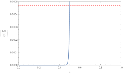
Figure 2: $|\Delta{T}_{f}/{T}_{f}|$ vs the model parameter $n$ (blue solid curve), for Model IV: $f=-T+\beta_{1}\left(T^{2}+\beta_{2}T_{G}\right)^{n}$ with $\beta_{2}\approx-2.90$, and the upper bound for $|\Delta{T}_{f}/{T}_{f}|$ from (26) (red dashed line). As we observe, constraints from BBN require $n\lesssim 0.5$.

IV.0.5 Model V: $f=-T+\alpha\ln\beta_{1}\left(T^{2}+\beta_{2}T_{G}\right)^{n}$

The last model we examine is the logarithmic one, characterized by $f=-T+\alpha\ln\beta_{1}\left(T^{2}+\beta_{2}T_{G}\right)^{n}$, where $\beta_{1}$, $\beta_{2}$, $n$ are the free parameters. Repeating the above analysis we find

$$\!\!\!\!\!\!\frac{\Delta T_{f}}{T_{f}}=\left(10c_{q}\zeta T_{f}^{7}\right)^{-1}H_{0}^{2}\Omega_{DE0}\Big{\{}\ln\beta_{1}+n\left[\ln 12\right.\\ \left.\ \ \left.+4\ln\left(\zeta T_{f}^{2}\right)+\ln\left(3\!-\!2\beta_{2}\right)\right.\right.\\ \left.\ \ \ \ \ \ \ \ \ \ \ \ \ \ \ \ -2\left(3\!-\!2\beta_{2}\right)^{-2}\left(18\!-\!39\beta_{2}\!+\!18\beta_{2}^{2}\right)\right]\Big{\}}\\ \!\cdot\Big{\{}\ln\beta_{1}+n\left\{\ln 12+2\ln(H_{0})+\ln[(3\!+\!2\beta_{2})H_{0}^{2}\!+\!2\beta_{2}\dot{H}_{0}]\right.\\ \left.\left.-2\left[\left(3+2\beta_{2}\right)H_{0}^{2}+2\beta_{2}\dot{H}_{0}\right]^{-2}\left[\left(18+15\beta_{2}+2\beta_{2}^{2}\right)H_{0}^{4}\right.\right.\right.\\ \left.\left.+\beta_{2}\left(27\!+\!12\beta_{2}\right)H_{0}^{2}\dot{H}_{0}\!+\!6\beta_{2}^{2}\dot{H}_{0}^{2}\!+\!2\beta_{2}^{2}H_{0}\ddot{H}_{0}\right]\right\}\!\!\Big{\}}^{-1},$$ (38)

where using relation (27) we find

$$\!\!\!\!\!\alpha=-6H_{0}^{2}\Omega_{DE0}\Big{\{}\ln\beta_{1}+n\Big{\{}\ln 12+2\ln(H_{0})\\ \left.\left.+\ln\left[\left(3\!+\!2\beta_{2}\right)H_{0}^{2}\!+\!2\beta_{2}\dot{H}_{0}\right]\right.\right.\\ \left.\left.-2\left[(3\!+\!2\beta_{2})H_{0}^{2}+2\beta_{2}\dot{H}_{0}\right]^{-2}\Big{[}(18\!+\!15\beta_{2}\!+\!2\beta_{2}^{2})H_{0}^{4}\right.\right.\\ +\beta_{2}\left(27\!+\!12\beta_{2}\right)H_{0}^{2}\dot{H}_{0}+6\beta_{2}^{2}\dot{H}_{0}^{2}+2\beta_{2}^{2}H_{0}\ddot{H}_{0}\Big{]}\Big{\}}\Big{\}}^{-1}.$$ (39)

We consider the values $\beta_{1}=0.001~{}{\rm GeV}^{-4n}$, $\beta_{2}\approx-2.9$ and we find that $n$ is allowed to take every value apart from $-0.0003$ and a very small region around it, since (38) diverges. Moreover, $\alpha$ is allowed to take every value apart from $0$, which is the value it obtains using the above narrow window for $n$. Using the same considerations as the above models, we find that for $\beta_{1}=0.001~{}{\rm GeV}^{-4n}$, $\beta_{2}=-2$ the value of $n$ is allowed to take every value apart from $-0.012$ and $a$ every value but $0$. Similarly, for $\beta_{1}=0.001~{}{\rm GeV}^{-4n}$, $\beta_{2}=-1$ we find that $n\neq-0.018$ and $a\neq 0$, while for $\beta_{1}=0.001~{}{\rm GeV}^{-4n}$, $\beta_{2}=1$ we find $n\neq-0.018$ and $a\neq 0$.

As an example, in Fig. 3 we present $|\Delta T_{f}/T_{f}|$ from (38) as a function of the model parameter $n$. The model parameter $n$ is allowed to take all possible values except those values around a very small region centered at $-0.0003$, in which (38) diverges. Hence, we conclude that the logarithmic $f(T,T_{G})$ model can easily satisfy the BBN bounds.

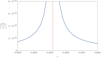
Figure 3: $|\Delta T_{f}/T_{f}|$ vs the model parameter $n$ (blue solid curve), for Model V: $f=-T+\alpha\ln\beta_{1}\left(T^{2}+\beta_{2}T_{G}\right)^{n}$, choosing $\beta_{1}=0.001~{}{\rm GeV}^{-4n}$, $\beta_{2}\approx-2.7$. The vertical dashed line at $n-0.0003$ denotes the point where (38) diverges.

V Conclusions

Modified gravity aims to provide explanations for various epochs of the Universe evolution, and at the same time to improve the renormalizability issues of General Relativity. Nevertheless, despite the specific advantages at a given era of the cosmological evolution one should be very careful not to spoil other, well understood and significantly constrained, phases, such as the Big Bang Nucleosynthesis (BBN) one.

In particular, there are many modified gravity models, which are constructed phenomenologically in order to be able to describe the late-time universe evolution at both background and perturbation level. Typically, these models are confronted with observational data such as Supernovae Type Ia (SNIa), Baryonic Acoustic Oscillations (BAO), Cosmic Microwave Background (CMB), Cosmic Chronometers (CC), Gamma-ray Bursts (GRB), growth data, etc. The problem is that although modified gravity scenarios, through the extra terms they induce, are very efficient in describing the late-time universe, quite often they induce significant terms at early times too, and thus spoiling the early-time evolution, such as the BBN phase, in which the concordance cosmological paradigm is very successful. Hence, independently of the late-universe successes that a modified gravity model may have, one should always examine whether the model can pass the BBN constraints too.

In the present work we confronted one interesting class of gravitational modification, namely $f(T,T_{G})$ gravity, with BBN requirements. The former is obtained using both the torsion scalar, as well as the teleparallel equivalent of the Gauss-Bonnet term, in the Lagrangian. Hence, one obtains modified Friedmann equations in which the extra torsional terms constitutes an effective dark energy sector.

We started by calculating the deviations of the freeze-out temperature $T_{f}$, caused by the extra torsion terms, in comparison to $\Lambda$CDM paradigm. We imposed five specific $f(T,T_{G})$ models that have been proposed in the literature in phenomenological grounds, i.e. in order to be able to describe the late-time evolution and lead to acceleration without an explicit cosmological constant. Hence, we extracted the constraints on the model parameters in order for the ratio $|\Delta T_{f}/T_{f}|$ to satisfy the BBN bound $\left|\frac{\Delta{T}_{f}}{{T}_{f}}\right|<4.7\times 10^{-4}$. As we found, in most of the models the involved parameters are bounded in a narrow window around their General Relativity values, as expected. However, the logarithmic model can easily satisfy the BBN constraints for large regions of the model parameters, which acts as an advantage for this scenario.

We stress here that we did not fix the cosmological parameters to their General Relativity values, on the contrary we left them completely free and we examined which parameter regions are allowed if we want the models to pass the BBN constraints. The fact that in most models the parameter regions are constrained to a narrow window around their General Relativity values was in some sense expected, but in general is not guaranteed or known a priori, since many modified gravity models are completely excluded under the BBN analysis since for all parameter regions their early-universe effect is huge.

In conclusion, $f(T,T_{G})$ gravity, apart from having interesting cosmological implications both in inflationary and late-time phase, possesses particular sub-classes that can safely pass BBN bounds, nevertheless the torsional modification is constrained in narrow windows around the General Relativity values. This feature should be taken into account in future model building.

References

(1)
K. S. Stelle,
Phys. Rev. D 16, 953 (1977).
(2)
A. Addazi, J. Alvarez-Muniz, R. A. Batista, G. Amelino-Camelia, V. Antonelli,
M. Arzano, M. Asorey, et al.
[arXiv:2111.05659 [hep-ph]].
(3)
S. Nojiri and S. D. Odintsov,
Phys. Rept. 505, 59 (2011)
[arXiv:1011.0544 [gr-qc]].
(4)
T. Clifton, P. G. Ferreira, A. Padilla and C. Skordis,
Phys. Rept. 513, 1 (2012)
[arXiv:1106.2476 [astro-ph.CO]].
(5)
S. Nojiri, S. D. Odintsov and V. K. Oikonomou,
Phys. Rept. 692, 1-104 (2017)
[arXiv:1705.11098 [gr-qc]].
(6)
E. N. Saridakis et al. [CANTATA],
[arXiv:2105.12582 [gr-qc]].
(7)
M. Ishak,
Living Rev. Rel. 22, no.1, 1 (2019)
[arXiv:1806.10122 [astro-ph.CO]].
(8)
E. Abdalla, G. Franco Abellán, A. Aboubrahim, A. Agnello, et
al.
JHEAp 34, 49-211 (2022)
[arXiv:2203.06142 [astro-ph.CO]].
(9)
A. A. Starobinsky,
Phys. Lett. B 91, 99 (1980).
(10)
S. Capozziello,
Int. J. Mod. Phys. D 11, 483 (2002),
[arXiv:gr-qc/0201033].
(11)
A. De Felice and S. Tsujikawa,
Living Rev. Rel. 13, 3 (2010)
[arXiv:1002.4928 [gr-qc]].
(12)
I. Antoniadis, J. Rizos and K. Tamvakis,
Nucl. Phys. B 415, 497 (1994).
(13)
S. Nojiri and S. D. Odintsov,
Phys. Lett. B 631, 1 (2005),
[arXiv:hep-th/0508049].
(14)
A. De Felice and S. Tsujikawa,
Phys. Lett. B 675, 1 (2009),
[arXiv:0810.5712].
(15)
Z. Yousaf, M. Z. Bhatti, S. Khan and P. K. Sahoo,
Phys. Dark Univ. 36, 101015 (2022)
[arXiv:2112.00575 [gr-qc]].
(16)
C. Erices, E. Papantonopoulos and E. N. Saridakis,
Phys. Rev. D 99, no.12, 123527 (2019)
[arXiv:1903.11128 [gr-qc]].
(17)
M. Marciu,
Phys. Rev. D 101, no.10, 103534 (2020)
[arXiv:2003.06403 [gr-qc]].
(18)
J. B. Jiménez and A. Jiménez-Cano,
JCAP 01, 069 (2021)
[arXiv:2009.08197 [gr-qc]].
(19)
D. Lovelock,
J. Math. Phys. 12, 498 (1971).
(20)
N. Deruelle and L. Farina-Busto,
Phys. Rev. D 41, 3696 (1990).
(21)
P. D. Mannheim and D. Kazanas,
Astrophys. J. 342, 635 (1989).
(22)
G. W. Horndeski,
Int. J. Theor. Phys. 10, 363-384 (1974).
(23)
C. Deffayet, G. Esposito-Farese and A. Vikman,
Phys. Rev. D 79, 084003 (2009),
[arXiv:0901.1314].
(24)
G. R. Bengochea and R. Ferraro,
Phys. Rev. D 79, 124019 (2009)
[arXiv:0812.1205 [astro-ph]].
(25)
Y. F. Cai, S. Capozziello, M. De Laurentis and E. N. Saridakis,
Rept. Prog. Phys. 79, no.10, 106901 (2016)
[arXiv:1511.07586 [gr-qc]].
(26)
G. Kofinas and E. N. Saridakis,
Phys. Rev. D 90, 084044 (2014)
[arXiv:1404.2249 [gr-qc]].
(27)
G. Kofinas, G. Leon and E. N. Saridakis,
Class. Quant. Grav. 31, 175011 (2014)
[arXiv:1404.7100 [gr-qc]].
(28)
G. Kofinas and E. N. Saridakis,
Phys. Rev. D 90, 084045 (2014)
[arXiv:1408.0107 [gr-qc]].
(29)
S. Bahamonde, C. G. Böhmer and M. Wright,
Phys. Rev. D 92, no.10, 104042 (2015)
[arXiv:1508.05120 [gr-qc]].
(30)
S. Bahamonde and S. Capozziello,
Eur. Phys. J. C 77, no.2, 107 (2017)
[arXiv:1612.01299 [gr-qc]].
(31)
C. Q. Geng, C. C. Lee, E. N. Saridakis and Y. P. Wu,
Phys. Lett. B 704, 384-387 (2011)
[arXiv:1109.1092 [hep-th]].
(32)
S. H. Chen, J. B. Dent, S. Dutta and E. N. Saridakis,
Phys. Rev. D 83, 023508 (2011)
[arXiv:1008.1250 [astro-ph.CO]].
(33)
P. Wu and H. W. Yu,
Phys. Lett. B 693, 415 (2010)
[arXiv:1006.0674 [gr-qc]].
(34)
J. B. Dent, S. Dutta and E. N. Saridakis,
JCAP 01, 009 (2011)
[arXiv:1010.2215 [astro-ph.CO]].
(35)
R. Myrzakulov,
Eur. Phys. J. C 71, 1752 (2011)
[arXiv:1006.1120 [gr-qc]].
(36)
R. Zheng and Q. G. Huang,
JCAP 03, 002 (2011)
[arXiv:1010.3512 [gr-qc]].
(37)
N. Tamanini and C. G. Boehmer,
Phys. Rev. D 86, 044009 (2012)
[arXiv:1204.4593 [gr-qc]].
(38)
K. Bamba, R. Myrzakulov, S. Nojiri and S. D. Odintsov,
Phys. Rev. D 85, 104036 (2012)
[arXiv:1202.4057 [gr-qc]].
(39)
H. Dong, Y. b. Wang and X. h. Meng,
Eur. Phys. J. C 72, 2002 (2012)
[arXiv:1203.5890 [gr-qc]].
(40)
K. Karami and A. Abdolmaleki,
JCAP 04, 007 (2012)
[arXiv:1201.2511 [gr-qc]].
(41)
D. Liu and M. J. Reboucas,
Phys. Rev. D 86, 083515 (2012)
[arXiv:1207.1503 [astro-ph.CO]].
(42)
G. Otalora,
JCAP 07, 044 (2013)
[arXiv:1305.0474 [gr-qc]].
(43)
Y. C. Ong, K. Izumi, J. M. Nester and P. Chen,
Phys. Rev. D 88, 024019 (2013)
[arXiv:1303.0993 [gr-qc]].
(44)
P. Chen, K. Izumi, J. M. Nester and Y. C. Ong,
Phys. Rev. D 91, no.6, 064003 (2015)
[arXiv:1412.8383 [gr-qc]].
(45)
G. Farrugia and J. Levi Said,
Phys. Rev. D 94, no.12, 124054 (2016)
[arXiv:1701.00134 [gr-qc]].
(46)
C. Bejarano, R. Ferraro and M. J. Guzmán,
Eur. Phys. J. C 77, no.12, 825 (2017)
[arXiv:1707.06637 [gr-qc]].
(47)
M. Hohmann, L. Jarv and U. Ualikhanova,
Phys. Rev. D 96, no.4, 043508 (2017)
[arXiv:1706.02376 [gr-qc]].
(48)
S. Bahamonde, C. G. Böhmer and M. Krššák,
Phys. Lett. B 775, 37-43 (2017)
[arXiv:1706.04920 [gr-qc]].
(49)
H. Abedi, S. Capozziello, R. D’Agostino and O. Luongo,
Phys. Rev. D 97, no.8, 084008 (2018)
[arXiv:1803.07171 [gr-qc]].
(50)
A. Golovnev and T. Koivisto,
JCAP 11, 012 (2018)
[arXiv:1808.05565 [gr-qc]].
(51)
M. Krssak, R. J. van den Hoogen, J. G. Pereira, C. G. Böhmer and A. A. Coley,
Class. Quant. Grav. 36, no.18, 183001 (2019)
[arXiv:1810.12932 [gr-qc]].
(53)
Y. F. Cai, M. Khurshudyan and E. N. Saridakis,
Astrophys. J. 888, 62 (2020)
[arXiv:1907.10813 [astro-ph.CO]].
(54)
M. Caruana, G. Farrugia and J. Levi Said,
Eur. Phys. J. C 80, no.7, 640 (2020)
[arXiv:2007.09925 [gr-qc]].
(55)
X. Ren, T. H. T. Wong, Y. F. Cai and E. N. Saridakis,
Phys. Dark Univ. 32, 100812 (2021)
[arXiv:2103.01260 [astro-ph.CO]].
(56)
R. Briffa, C. Escamilla-Rivera, J. Said Levi, J. Mifsud and N. L. Pullicino,
Eur. Phys. J. Plus 137, no.5, 532 (2022)
[arXiv:2108.03853 [astro-ph.CO]].
(57)
D. Benisty, E. I. Guendelman, A. van de Venn, D. Vasak, J. Struckmeier and
H. Stoecker,
Eur. Phys. J. C 82, no.3, 264 (2022)
[arXiv:2109.01052 [astro-ph.CO]].
(58)
K. F. Dialektopoulos, J. L. Said and Z. Oikonomopoulou,
Eur. Phys. J. C 82, no.3, 259 (2022)
[arXiv:2112.15045 [gr-qc]].
(59)
G. Papagiannopoulos, S. Basilakos and E. N. Saridakis,
[arXiv:2202.10871 [gr-qc]].
(60)
T. Papanikolaou, C. Tzerefos, S. Basilakos and E. N. Saridakis,
[arXiv:2205.06094 [gr-qc]].
(61)
T. Wang,
Phys. Rev. D 84, 024042 (2011)
[arXiv:1102.4410 [gr-qc]].
(62)
C. G. Boehmer, A. Mussa and N. Tamanini,
Class. Quant. Grav. 28, 245020 (2011)
[arXiv:1107.4455 [gr-qc]].
(63)
R. Ferraro and F. Fiorini,
Phys. Rev. D 84, 083518 (2011)
[arXiv:1109.4209 [gr-qc]].
(64)
X. h. Meng and Y. b. Wang,
Eur. Phys. J. C 71, 1755 (2011)
[arXiv:1107.0629 [astro-ph.CO]].
(65)
M. E. Rodrigues, M. J. S. Houndjo, D. Saez-Gomez and F. Rahaman,
Phys. Rev. D 86, 104059 (2012)
[arXiv:1209.4859 [gr-qc]].
(66)
M. E. Rodrigues, M. J. S. Houndjo, J. Tossa, D. Momeni and R. Myrzakulov,
JCAP 11, 024 (2013)
[arXiv:1306.2280 [gr-qc]].
(67)
G. G. L. Nashed,
Phys. Rev. D 88, 104034 (2013)
[arXiv:1311.3131 [gr-qc]].
(68)
C. Bejarano, R. Ferraro and M. J. Guzmán,
Eur. Phys. J. C 75, 77 (2015)
[arXiv:1412.0641 [gr-qc]].
(69)
A. Das, F. Rahaman, B. K. Guha and S. Ray,
Astrophys. Space Sci. 358, no.2, 36 (2015)
[arXiv:1507.04959 [gr-qc]].
(70)
Z. F. Mai and H. Lu,
Phys. Rev. D 95, no.12, 124024 (2017)
[arXiv:1704.05919 [hep-th]].
(71)
G. Mustafa, G. Abbas and T. Xia,
Chin. J. Phys. 60, 362-378 (2019)
(72)
G. G. L. Nashed and S. Capozziello,
Eur. Phys. J. C 80, no.10, 969 (2020)
[arXiv:2010.06355 [gr-qc]].
(73)
C. Pfeifer and S. Schuster,
Universe 7, no.5, 153 (2021)
[arXiv:2104.00116 [gr-qc]].
(74)
X. Ren, Y. Zhao, E. N. Saridakis and Y. F. Cai,
JCAP 10, 062 (2021)
[arXiv:2105.04578 [astro-ph.CO]].
(75)
S. Bahamonde, A. Golovnev, M. J. Guzmán, J. L. Said and C. Pfeifer,
JCAP 01, no.01, 037 (2022)
[arXiv:2110.04087 [gr-qc]].
(76)
S. Bahamonde, L. Ducobu and C. Pfeifer,
JCAP 04, no.04, 018 (2022)
[arXiv:2201.11445 [gr-qc]].
(77)
Y. Huang, J. Zhang, X. Ren, E. N. Saridakis and Y. F. Cai,
[arXiv:2204.06845 [astro-ph.CO]].
(78)
Y. Zhao, X. Ren, A. Ilyas, E. N. Saridakis and Y. F. Cai,
[arXiv:2204.11169 [gr-qc]]
(79)
J. Bernstein, L. S. Brown and G. Feinberg,
Rev. Mod. Phys. 61, 25 (1989).
(80)
E. W. Kolb and M. S. Turner,
Front. Phys. 69, 1-547 (1990).
(81)
K. A. Olive, G. Steigman and T. P. Walker,
Phys. Rept. 333, 389-407 (2000)
[arXiv:astro-ph/9905320 [astro-ph]].
(82)
R. H. Cyburt, B. D. Fields, K. A. Olive and T. H. Yeh,
Rev. Mod. Phys. 88, 015004 (2016)
[arXiv:1505.01076 [astro-ph.CO]].
(83)
P. Asimakis, S. Basilakos, N. E. Mavromatos and E. N. Saridakis,
Phys. Rev. D 105, no.8, 8 (2022)
[arXiv:2112.10863 [gr-qc]].
(84)
D. F. Torres, H. Vucetich and A. Plastino,
Phys. Rev. Lett. 79, 1588-1590 (1997)
[arXiv:astro-ph/9705068 [astro-ph]].
(85)
G. Lambiase,
Phys. Rev. D 72, 087702 (2005)
[arXiv:astro-ph/0510386 [astro-ph]].
(86)
G. Lambiase,
Phys. Rev. D 83, 107501 (2011).
(87)
F. K. Anagnostopoulos, V. Gakis, E. N. Saridakis and S. Basilakos,
[arXiv:2205.11445 [gr-qc]].
(88)
A. Coc, E. Vangioni-Flam, P. Descouvemont, A. Adahchour and C. Angulo,
Astrophys. J. 600, 544-552 (2004)
[arXiv:astro-ph/0309480 [astro-ph]].
(89)
K. A. Olive, E. Skillman and G. Steigman,
Astrophys. J. 483, 788 (1997)
[arXiv:astro-ph/9611166 [astro-ph]].
(90)
Y. I. Izotov and T. X. Thuan,
Astrophys. J. 500, 188 (1998).
(91)
B. D. Fields and K. A. Olive,
Astrophys. J. 506, 177 (1998)
[arXiv:astro-ph/9803297 [astro-ph]].
(92)
Y. I. Izotov, F. H. Chaffee, C. B. Foltz, R. F. Green, N. G. Guseva and
T. X. Thuan,
Astrophys. J. 527, 757-777 (1999)
[arXiv:astro-ph/9907228 [astro-ph]].
(93)
D. Kirkman, D. Tytler, N. Suzuki, J. M. O’Meara and D. Lubin,
Astrophys. J. Suppl. 149, 1 (2003)
[arXiv:astro-ph/0302006 [astro-ph]].
(94)
Y. I. Izotov and T. X. Thuan,
Astrophys. J. 602, 200-230 (2004)
[arXiv:astro-ph/0310421 [astro-ph]].
(95)
N. Aghanim et al. [Planck],
Astron. Astrophys. 641, A6 (2020)
[arXiv:1807.06209 [astro-ph.CO]].