Non-Hermitian dynamics of a two-spin system with $\mathcal{PT}$ symmetry

Abstract

A system of interacting spins that are under the influence of spin-polarized currents can be described using a complex functional, or a non-Hermitian (NH) Hamiltonian. We study the dynamics of two exchange-coupled spins on the Bloch sphere. In the case of currents leading to $\mathcal{PT}$ symmetry, an exceptional point that survives also in the nonlinear system is identified. The nonlinear system is bistable for small currents and it exhibits stable oscillating motion or it can relax to a fixed point. The oscillating motion of the two spins is akin to synchronised spin-torque oscillators. For the full nonlinear system, we derive two conserved quantities that furnish a geometric description of the spin trajectories in phase space and indicate stability of the oscillating motion. Our analytical results provide tools for the description of the dynamics of NH systems that are defined on the Bloch sphere.

I Introduction

Effective non-Hermitian (NH) Hamiltonians 2018_NatPhys_ElGanainyMakris ; 2021_RevModPhys_Bergholtz have been employed for the description of classical 2016_RMP_KonotopJiankeZezyulin ; 2019_Science_MiriAlu and quantum systems 2007_RepProgPhys_Bender ; 2009_JPA_Rotter that are coupled to the environment by dissipative or other forces. The observation that NH Hamiltonians that are invariant under the combination of parity and time reversal ($\mathcal{PT}$) foster real spectra 1998_PRL_BenderBoettcher ; 2007_RepProgPhys_Bender has led to a series of theoretical and experimental studies. Significant amount of work has focused on optical systems with balanced gain and loss such as in optical beam propagation 2010_NatPhys_RueterMakris and single-mode lasers 2014_Science_FengWongMa . More recently, magnetic systems with $\mathcal{PT}$ symmetry have been proposed 2016_PRB_GaldaVinokur ; 2017_SciRep_GaldaVinokur ; 2019_SciRep_GaldaVinokur ; 2020_PhysD_Barashenkov and systems with gain and loss 2018_PRL_YangWang ; 2021_PRAppl_WangGuoBerakdar ; 2021_arXiv_WittrockPerna ; 2022_arXiv_DengLiFlebus , with the latter reports focusing on degeneracies, called exceptional points (EP), in the spectrum of the linear system, were the sensitivity of the system is enhanced. Effects of EPs were demonstrated for magnonic systems which possess two different loss factors 2019_SciAdv_LiuSun .

Spin systems are studied extensively in relation to magnetic materials HubertSchaefer motivated by applications in magnetic recording, nanoscopic sensors, antennas 2017_NatRevMater_FertReyrenCros , computing applications and neural network implementations 2016_IEEE_GrollierQuerliozStiles . Probing ferromagnets (and other magnetic materials) is done most efficiently by spin torques that are due to a spin-polarized current. This acts on the magnetic moments in the material in a way that may combine energy gain and loss and it drives magnetization dynamics 2008_JMMM_BerkovMiltat . Spin-transfer torque nano-oscillators (STNO) can be constructed that give rise to magnetization oscillators due to injection of dc spin-polarized current RussekRippardCecil_2010 . A $\mathcal{PT}$-symmetric system of this kind with a single spin was studied in Ref. 2016_PRB_GaldaVinokur . The synchronization of chains of STNOs in order to produce large power is a main challenge in this area 2017_NatPhys_AwadAkerman ; 2017_NatComms_LebrunCros .

We propose a $\mathcal{PT}$-symmetric system of two interacting spins or magnetic moments that can realistically be constructed when we invoke suitable spin torque effects. We show that this is described by a complex function instead of a real Hamiltonian. This gives a paradigm of a realistic nontrivial system on the Bloch sphere. We show that the nonlinear system exhibits oscillating motion that is connected with the real eigenvalues of the linearized system. For the full nonlinear system, we derive two conserved quantities that make an explicit connection between the NH system and the Hamiltonian one, and they also furnish a geometric description of the spin trajectories in phase space.

Single spin systems are crucial for quantum computing, and observations on a $\mathcal{PT}$-symmetric single-spin system have been reported 2019_Science_WuLiu . An effective spin Hamiltonian is obtained in various physical systems. An example is a spin Hamiltonian obtained for qubits in an exciton polariton condensate, which are externally controllable by applied laser pulses and are coupled via a coherent tunneling term 2020_NPJ_GhoshLiew . Finally, it is well-known that the possible quantum states for a single qubit can be represented on a Bloch sphere. Our analytical results on complex Hamiltonians could provide tools for a more complete and elegant description of the dynamics of interacting spins on the Bloch sphere in magnetic and other systems.

The paper is organised as follows. In Sec. II, we give the formulation of a spin system using a complex functional. In Sec. III, we give the complex function for a system of two spins coupled by exchange. In Sec. IV, we give analytically simple periodic solutions for the spin dynamics. In Sec. V, we derive two conserved quantities and give their geometric meaning. Sec. VI contains our concluding remarks.

II A complex function for spins

We consider a spin system described via the magnetization vector $\bm{m}=(m_{x},m_{y},m_{z})$ assumed to have a fixed length normalized to unity, $|\bm{m}|=1$. If $E$ denotes the magnetic energy, the conservative torque on the magnetization is $\bm{f}=-\partial E/\partial\bm{m}$. A polarized spin current that is injected in the system may produce an additional torque and the normalised equation of motion is 2008_JMMM_BerkovMiltat

$$\frac{\partial\bm{m}}{\partial t}=\bm{m}\times\frac{\partial E}{\partial\bm{m}}+\alpha\,\bm{m}\times\frac{\partial\bm{m}}{\partial t}-\beta\,\bm{m}\times(\bm{m}\times\bm{p}),$$ (1)

where $\bm{p}$ is the spin current polarization, $\beta$ is a parameter proportional to the polarized current, and we have included a Gilbert damping term with parameter $\alpha$. In the case of a ferromagnetic material, the time variable is scaled to $1/(\gamma\mu_{0}M_{s})$ where $M_{s}$ is the saturation magnetization and $\gamma$ is the gyromagnetic ratio.

The stereographic projection from the unit sphere $|\bm{m}|=1$ to the complex plane is given by the complex variable

$$\Omega=\frac{m_{x}+im_{y}}{1+m_{z}}.$$ (2)

This can be inverted to give the magnetization components

$$m_{x}=\frac{\Omega+\overline{\Omega}}{1+\Omega\overline{\Omega}},\;\;m_{y}=\frac{1}{i}\frac{\Omega-\overline{\Omega}}{1+\Omega\overline{\Omega}},\;\;m_{z}=\frac{1-\Omega\overline{\Omega}}{1+\Omega\overline{\Omega}},$$ (3)

where the bar denotes complex conjugation. The stereographic projection variable will make manifest the non-Hermiticity of the model and it will be central in the formulation of the present work.

The equation of motion for $\Omega$, equivalent to Eq. (1), reads

$$(i+\alpha)\,\dot{\Omega}=-\frac{1}{2}\,(1+\Omega\overline{\Omega})^{2}\,\left(\frac{\partial E}{\partial\overline{\Omega}}+i\beta\,\frac{\partial E_{\rm ST}}{\partial\overline{\Omega}}\right)$$ (4)

where we have defined the function

$$E_{\rm ST}=-\bm{m}\cdot\bm{p}.$$ (5)

Formula (4) suggests the definition of a complex function that includes the spin torque term,

$$F=E+i\beta E_{\rm ST},$$ (6)

so that the equation of motion for $\Omega$ takes the compact form

$$(i+\alpha)\,\dot{\Omega}=-\frac{1}{2}\,(1+\Omega\overline{\Omega})^{2}\,\frac{\partial F}{\partial\overline{\Omega}}.$$ (7)

The function $F$ will be called the complex Hamiltonian.

As a basic example, if we have an external magnetic field $\bm{h}=(0,0,h)$ giving rise to the energy $E=-\bm{m}\cdot\bm{h}$, and the spin polarization is $\bm{p}=(0,0,1)$, then $F=-(h+i\beta)m_{z}$ and the equation of motion is

$$(i+\alpha)\,\dot{\Omega}=-(h+i\beta)\Omega.$$ (8)

III Two exchange-coupled spins

We proceed to consider two magnetization vectors or spins interacting via exchange. These may represent two domains or layers in a magnetic material 2020_NatMater_LegrandCrosFert , or two effective spins in another physical system.

We denote the two vectors by $\bm{m}_{1},\bm{m}_{2}$ and assume that they have equal length, $|\bm{m}_{1}|=|\bm{m}_{2}|=1$. Except for the exchange interaction, we include an easy-axis anisotropy along $z$, and an external field $\bm{h}=h\bm{\hat{e}}_{z}$. The energy is

$$E=-J\,\bm{m}_{1}\cdot\bm{m}_{2}-\frac{\kappa}{2}\left[\left(m_{1,z}\right)^{2}+\left(m_{2,z}\right)^{2}\right]-h\,(m_{1,z}+m_{2,z})$$ (9)

where $J>0,\,\kappa>0$ are the exchange and anisotropy parameters respectively, and $m_{1,z},m_{2,z}$ denote the $z$ components of the two vectors. We further consider that spin-polarized currents are injected in the two domains $\bm{m}_{1},\bm{m}_{2}$, with polarization in two opposite directions, $\bm{p}=\pm\bm{\hat{e}}_{z}$. (Such a strategy for achieving $\mathcal{PT}$ symmetry is mentioned in 2016_RMP_KonotopJiankeZezyulin and attributted to 2016_Gaididei .) The opposite polarizations could be achieved, e.g., in the case of two coupled ferromagnetic layers, by injecting a current through the layer separating the two magnetic layers 2021_PRAppl_WangGuoBerakdar , or by two different currents through layers adjacent to each one of the magnetic layers. Spin current polarization with a component perpendicular to the sample plane was recently demonstrated 2022_NatElectr_BoseSchreiberRalph ; 2022_NatElectr_BoseRalph . The equations of motion are

$$\begin{split}\dot{\bm{m}}_{1}&=-\bm{m}_{1}\times\bm{f}_{1}+\alpha\bm{m}_{1}\times\dot{\bm{m}}_{1}-\beta\bm{m}_{1}\times(\bm{m}_{1}\times\bm{\hat{e}}_{z})\\ \dot{\bm{m}}_{2}&=-\bm{m}_{2}\times\bm{f}_{2}+\alpha\bm{m}_{2}\times\dot{\bm{m}}_{2}+\beta\bm{m}_{2}\times(\bm{m}_{2}\times\bm{\hat{e}}_{z})\end{split}$$ (10)

where the dot denotes time differentiation and the effective fields are

$$\begin{split}\bm{f}_{1}&=-\frac{\partial E}{\partial\bm{m}_{1}}=J\bm{m}_{2}+\kappa\,m_{1,z}\bm{\hat{e}}_{z}+h\,\bm{\hat{e}}_{z},\\ \bm{f}_{2}&=-\frac{\partial E}{\partial\bm{m}_{2}}=J\bm{m}_{1}+\kappa\,m_{2,z}\bm{\hat{e}}_{z}+h\,\bm{\hat{e}}_{z}.\end{split}$$

We will assume in the following $h>0,\,\beta>0$. Eqs. (10) have four fixed points. Two fixed points correspond to both $\bm{m}_{1},\bm{m}_{2}$ pointing at the north or at the south pole,

$$\bm{m}_{1}=\bm{m}_{2}=\bm{\hat{e}}_{z}$$ (P1)

$$\bm{m}_{1}=\bm{m}_{2}=-\bm{\hat{e}}_{z}$$ (P2)

and two further fixed points correspond to the vectors pointing at opposite poles,

$$\bm{m}_{1}=\bm{\hat{e}}_{z},\quad\;\;\,\bm{m}_{2}=-\bm{\hat{e}}_{z}$$ (P3)

$$\bm{m}_{1}=-\bm{\hat{e}}_{z},\quad\bm{m}_{2}=\bm{\hat{e}}_{z}.$$ (P4)

For the study of the stability of the fixed points as well as for using the concepts of non-Hermiticity, we proceed to the formulation of the system using the stereographic projections (2) of each of the spins, denoted by $\Omega_{1},\Omega_{2}$. We write the complex Hamiltonian of Eq. (6) for the system of two spins,

$$\begin{split}F=&-J\,\bm{m}_{1}\cdot\bm{m}_{2}-\frac{\kappa}{2}\left[\left(m_{1,z}\right)^{2}+\left(m_{2,z}\right)^{2}\right]\\ &-h\,(m_{1,z}+m_{2,z})+i\beta\,(m_{2,z}-m_{1,z}).\end{split}$$ (11)

This can be written in terms of the stereographic variables using Eqs. (3). For example, the exchange term is

$$-J\bm{m}_{1}\cdot\bm{m}_{2}=2J\frac{(\Omega_{1}-\Omega_{2})(\overline{\Omega}_{1}-\overline{\Omega}_{2})}{(1+\Omega_{1}\overline{\Omega}_{1})(1+\Omega_{2}\overline{\Omega}_{2})}.$$ (12)

The equations of motion for $\Omega_{1},\Omega_{2}$, from Eq. (7), read

$$\begin{split}(i+\alpha)\,\dot{\Omega}_{1}=J\frac{1+\Omega_{1}\overline{\Omega}_{2}}{1+\Omega_{2}\overline{\Omega}_{2}}(\Omega_{2}-\Omega_{1})&-\kappa\frac{1-\Omega_{1}\overline{\Omega}_{1}}{1+\Omega_{1}\overline{\Omega}_{1}}\,\Omega_{1}\\ &-(h+i\beta)\Omega_{1}\\ (i+\alpha)\,\dot{\Omega}_{2}=J\frac{1+\overline{\Omega}_{1}\Omega_{2}}{1+\Omega_{1}\overline{\Omega}_{1}}(\Omega_{1}-\Omega_{2})&-\kappa\frac{1-\Omega_{2}\overline{\Omega}_{2}}{1+\Omega_{2}\overline{\Omega}_{2}}\,\Omega_{2}\\ &-(h-i\beta)\Omega_{2}.\end{split}$$ (13)

System (13) is $\mathcal{PT}$-symmetric when we neglect the damping term by setting $\alpha=0$. The terms with $\beta$ act as gain and loss, but note that not each separate one of them can be classified as giving only gain or only loss. This is unlike in previous works on magnetics 2015_PRB_LeeKottosShapiro ; 2018_PRL_YangWang ; 2021_PRAppl_WangGuoBerakdar ; 2022_arXiv_DengLiFlebus , where damping and anti-damping torques were assumed 2022_arXiv_HurstFlebus .

The solution of Eq. (13) $\Omega_{1}=0,\,\Omega_{2}=0$ corresponds to the fixed point (P1) where both vectors point at the north pole. We can study the behavior of the system close to the fixed point if we assume $|\Omega_{1}|,|\Omega_{2}|\ll 1$ and linearize the equations. We have the linearized system (for $\alpha=0$)

$$\begin{split}i\dot{\Omega}_{1}&=-(\omega_{0}+i\beta)\Omega_{1}+J\Omega_{2},\qquad\omega_{0}=J+\kappa+h\\ i\dot{\Omega}_{2}&=-(\omega_{0}-i\beta)\Omega_{2}+J\Omega_{1}\end{split}$$ (14)

that has the form of a standard linear $\mathcal{PT}$-symmetric dimer model. For $\beta\leq J$, we define an angle $\theta$ via

$$\sin\theta=\frac{\beta}{J},\qquad 0\leq\theta\leq\pi$$ (15)

and have a solution

$$\Omega_{1}=A\,e^{i\omega t},\quad\Omega_{2}=A\,e^{i\theta}\,e^{i\omega t},$$ (16)

with angular frequency

$$\omega=\omega_{0}-J\cos\theta.$$ (17)

This solution corresponds to a periodic motion of both spins with equal amplitudes $|\Omega_{1}|=|\Omega_{2}|$. Equivalently, one can say that the spins have equal $z$ components, $m_{1,z}=m_{2,z}$ while precession occurs around the $z$ axis.

For $\beta>J$, the angular frequency has an imaginary part,

$$\omega=\omega_{0}\pm iJ\sqrt{(\beta/J)^{2}-1},$$ (18)

which means that $|\Omega_{1}|,|\Omega_{2}|$ will generically grow in time and, thus, the fixed point is unstable. A corresponding analysis for the fixed point (P2) gives the same stability results, that is, precessional motion for $\beta\leq J$ and an instability for $\beta>J$.

In order to study the fixed point (P3), we use the transformation $\Psi_{2}=1/\overline{\Omega}_{2}$ for the second spin. Then, (P3) corresponds to $\Omega_{1}=0,\Psi_{2}=0$. The equations of motion (13) become (for $\alpha=0$)

$$\begin{split}i\,\dot{\Omega}_{1}=J\frac{1-\Omega_{1}\overline{\Psi}_{2}}{1+\Psi_{2}\overline{\Psi}_{2}}(\Omega_{1}+\Psi_{2})&-\kappa\frac{1-\Omega_{1}\overline{\Omega}_{1}}{1+\Omega_{1}\overline{\Omega}_{1}}\,\Omega_{1}-(h+i\beta)\Omega_{1}\\ i\,\dot{\Psi}_{2}=J\frac{\overline{\Omega}_{1}\Psi_{2}-1}{1+\Omega_{1}\overline{\Omega}_{1}}(\Omega_{1}+\Psi_{2})&-\kappa\frac{\Psi_{2}\overline{\Psi}_{2}-1}{\Psi_{2}\overline{\Psi}_{2}+1}\,\Psi_{2}-(h+i\beta)\Psi_{2}.\end{split}$$ (19)

In order to study stability, we assume $\Omega_{1},\Psi_{2}\ll 1$ and linearize the equations to obtain

$$\begin{split}i\dot{\Omega}_{1}&=(J-\kappa-h-i\beta)\Omega_{1}+J\Psi_{2}\\ i\dot{\Psi}_{2}&=(-J+\kappa-h-i\beta)\Psi_{2}-J\Omega_{1}.\end{split}$$ (20)

Assuming solutions

$$\Omega_{1}=A_{1}e^{i\omega t},\quad\Psi_{2}=\frac{1}{\overline{\Omega}_{2}}=A_{2}e^{i\omega t},$$

we obtain the condition

$$(\omega-h-i\beta)^{2}=\kappa(\kappa-2J).$$ (21)

In the case

$$\kappa\geq 2J\Rightarrow\omega=h\pm\sqrt{\kappa(\kappa-2J)}+i\beta,$$ (22)

we have that $i\omega$ has a negative real part, $-\beta$, giving asymptotic stability for every $\beta>0$. In the case

$$\kappa<2J\Rightarrow\omega=h+i\left[\beta\pm\sqrt{\kappa(2J-\kappa)}\right],$$ (23)

we have that

$$\beta\geq\sqrt{\kappa(2J-\kappa)}$$ (24)

gives asymptotic stability, while

$$\beta<\sqrt{\kappa(2J-\kappa)}$$ (25)

gives instability. The right side in Eq. (23) has a maximum equal to $J$ at $\kappa=J$. This means that, for $\beta>J$, the fixed point is stable for every value of $\kappa$.

Finally, for the fixed point (P4), we can follow a similar procedure and find that it is unstable for every value of $\beta>0,\,\kappa>0$. Table 1 summarizes the results for the stability of the fixed points.

	stable	unstable
P1	$\beta\leq J$	$\beta>J$
P2	$\beta\leq J$	$\beta>J$
P3	$\kappa\geq 2J$ or $\beta\geq\sqrt{\kappa(2J-\kappa)}$	$\kappa<2J$ and $\beta<\sqrt{\kappa(2J-\kappa)}$
P4	-	$\beta>0$

Table 1: Stability regimes for the four fixed points. The results of linear stability analysis agree with numerical simulation results for the nonlinear system. We are confined to the case $J,\beta>0$.

The linear stability results of this section determine cases where fixed points are unstable. On the other hand, in the cases where the linear system is stable (with a real frequency), no conclusive result can be drawn for the nonlinear system (as dictated by standard dynamical systems theory). Further study of the stability will be given in Sec. IV.2.

IV Nonlinear oscillations

IV.1 Amplitude and frequency

We proceed to study solutions of the nonlinear system (13). We start by assuming solutions of the form (16) that is, perfect oscillations where the two spins differ by a phase. Substituting in Eqs. (13), we obtain

$$|A|^{2} \left[J(1-e^{-i\theta})+\kappa+\omega-h-i\beta\right]$$

$$+\left[J(e^{i\theta}-1)-\kappa+\omega-h-i\beta\right]=0,$$

$$|A|^{2} \left[J(1-e^{i\theta})+\kappa+\omega-h+i\beta\right]$$

$$+\left[J(e^{-i\theta}-1)-\kappa+\omega-h+i\beta\right]=0.$$

The two equations are identical if condition (15) holds, and they reduce to

$$|A|^{2} \left[J(1-\cos\theta)+\kappa+(\omega-h)\right]$$

$$+ \left[J(1-\cos\theta)+\kappa-(\omega-h)\right]=0.$$

This obtains the angular frequency as a function of the amplitude (as expected for nonlinear oscillators),

$$\omega=\frac{1-|A|^{2}}{1+|A|^{2}}\left[J\,(1-\cos\theta)+\kappa\right]+h.$$ (26)

For the interpretation of this result, one should note that $(1-|A|^{2})/(1+|A|^{2})$ gives the $z$ component of $\bm{m}_{1},\bm{m}_{2}$. For every $\beta\leq J$, Eq. (15) gives two angles $\theta_{1},\theta_{2}$ with $\theta_{2}=\pi-\theta_{1}$ (assuming $\theta_{1}<\pi/2$) and thus two frequency values are given by (26). For $0\leq\theta=\theta_{1}\leq\pi/2$, we obtain an acoustic branch and for $\pi/2\leq\theta=\theta_{2}\leq\pi$, we obtain an optical branch. Related observations were reported in 2019_SciAdv_LiuSun for a passive magnonic system.

Eq. (15) implies an exceptional point at $\beta=J$ for the nonlinear system. This means that the system possesses periodic orbits for $\beta<J$ but these are not sustained for $\beta>J$. Furthermore, at $\beta=J$, Eq. (15) gives a single solution $\theta=\pi/2$, the two frequencies coalesce to a single one and we have only one nonlinear oscillation solution (16). The exceptional point of the nonlinear system coincides with that obtained for the linearized system (14). The stability of the periodic orbits in the nonlinear system will be studied numerically in the next subsection.

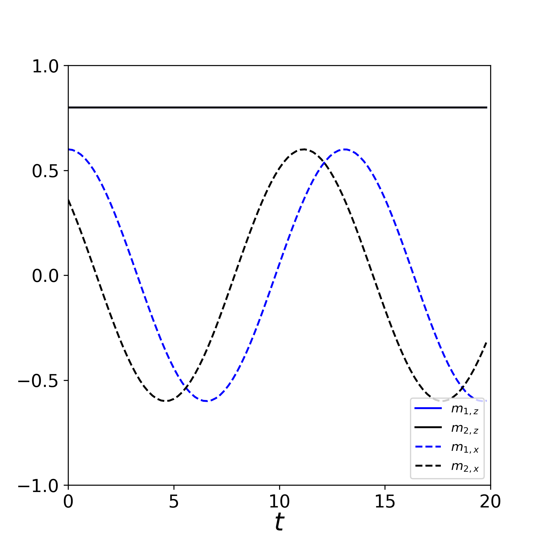
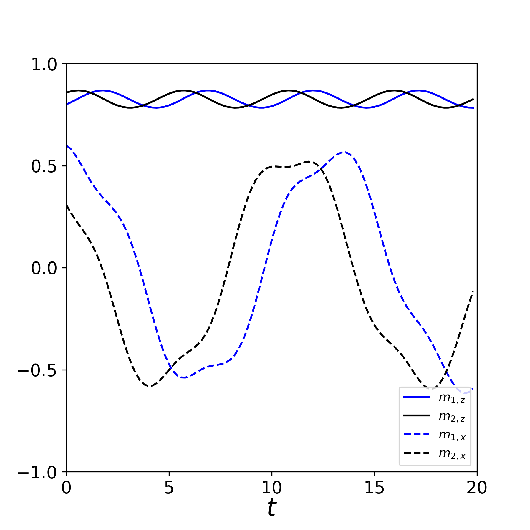
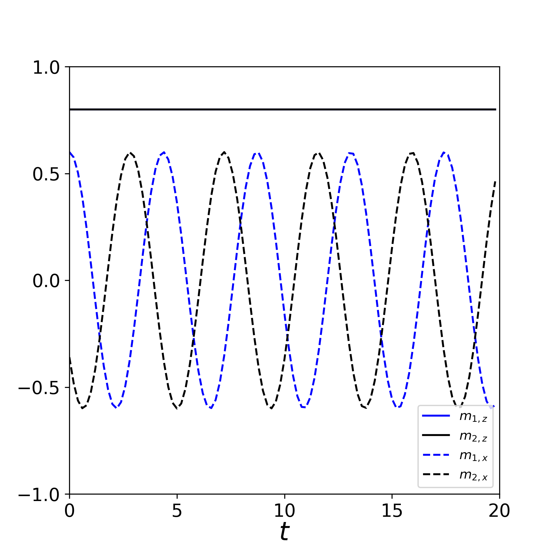
(a)          (b) (c)          (d)

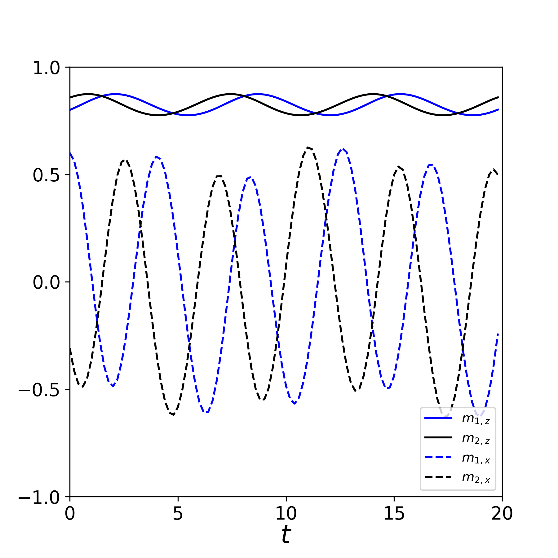
Figure 1: We simulate Eqs. (13) with parameters $J=1,\kappa=0.2,h=0$ and spin-torque parameter $\beta=0.8$. The first and the third components of the magnetization $m_{1,x}(t),m_{2,x}(t)$ and $m_{1,z}(t),m_{2,z}(t)$ are shown. (a) Using an initial condition that agrees with Eqs. (15) (for $\theta<\pi/2$) and (16), we obtain spin precession in the acoustic branch, that is, oscillations around the nonlinear eigenstate (16). (b) When we choose the initial condition close to the values used in (a), we obtain oscillations of the $z$ component of the spins in addition to precessional motion. (c) Using an initial condition that agrees with Eqs. (15) (for $\theta>\pi/2$) and (16), we obtain spin precession in the optical branch. (d) Similar simulation to (b) for the optical branch.

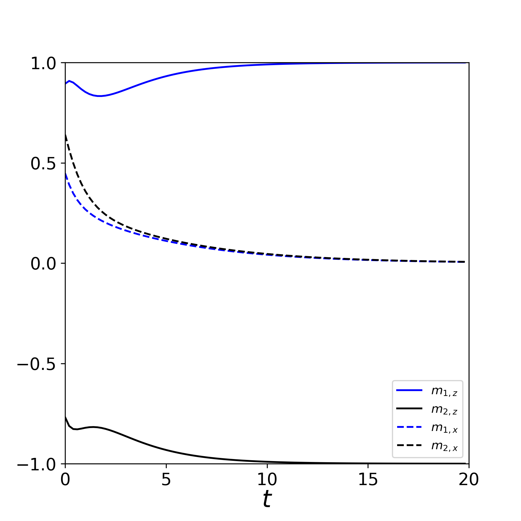
Figure 2: We use the same parameter values as in the simulation in Fig. 1 so that $\beta>\sqrt{\kappa(2J-\kappa)}=0.6$. We use an initial condition close to the fixed point (P3). We observe that the system goes asymptotically to this fixed point.

We conclude the subsection by making some further remarks on Eq. (26) and assuming $h=0$ for simplicity. The frequency is invariant under the transformation $A\to 1/A$. This corresponds to the invariance of the model under the transformation $m_{3}\to-m_{3}$. For small amplitude, $|A|\to 0$, the spins are close to the north pole of the Bloch sphere and Eq. (26) reduces to the result (17) of the linear model. The limit $|A|\to\infty$ is allowed and it corresponds to the spins being close to the south pole of the sphere. The frequency of oscillation has maximum absolute value for $\bm{m}$ close to the north ($A\to 0$) or the south pole ($|A|\to\infty$).

In the case that both spins point on the equator, $|A|=1$, there is no spin precession, $\omega=0$, according to Eq. (26) for $h=0$. Therefore, the configurations $\Omega_{2}=e^{i\theta}\Omega_{1}$, for $|\Omega_{1}|=|\Omega_{2}|=1$, give a continuum of fixed points of the system. These are additional to the four fixed points P1-P4 discussed in Sec. III. The new fixed points are obviously unstable, as any deviation from the equator would result in spin precession around the $z$ axis, that means, the spins would go away from their fixed point positions.

IV.2 Numerics

We simulate numerically the system when it is below the exceptional point, for $\beta<J$, and find that it follows the precessional eigenstates (16) of the nonlinear system if the initial spin configuration is prepared so that it agrees with Eqs. (15) and (16). Fig. 1a shows an example of spin precession for the acoustic branch. Fig. 1c shows an example of spin precession for the optical branch. The graphs show the $x$ and the $z$ components of the magnetization vector. The frequency of precession is given by Eq. (26) and the result is verified in the graphs by the periodicity of the $x$ components of the magnetization vectors.

Furthermore, for an initial condition that is close to the eigenstate (16), we obtain quasi-periodic motion where the $z$ components of the spins oscillate while the spins precess around the $z$ axis. An example is shown in Fig. 1b, for an initial condition close to the one that gave the acoustic branch periodic motion in Fig. 1a. Another example is shown in Fig. 1d, for an initial condition close to the one that gave the optical branch periodic motion in Fig. 1c. Two frequencies are involved in this motion. The precessional motion frequency is close to (26), while the periodicity of the oscillation of the $z$ component of the spin gives a second frequency apparently unrelated to the spin precession frequency.

For the simulations in Fig. 1, we have chosen parameter such that condition (24) is satisfied, and the system is expected to be bistable as inferred from Table 1. We run a further simulation using the same parameter set, but now choosing an initial condition close to the point (P3). We find that the system goes asymptotically to this fixed point, as shown in Fig. 2. This verifies the bistability of the system.

In the case that $\beta$ satisfies condition (25), only (P1), (P2) are stable. Starting from any initial condition the system goes into a periodic or a quasi periodic motion similar to those shown in Fig. 1.

Finally, when we cross the exceptional point, for $\beta>J$, the fixed points (P1), (P2) are unstable due to the imaginary part in the eigenvalues (18). Then, (P3) is the only stable fixed point and the system goes to that asymptotically from any initial condition.

We conclude the section with a note about the remarkable periodicity in the dynamics of this system. The quasi-periodic motion observed in many of the simulations, cannot be considered as direct consequencies of the results obtained in Sec. III for the linearized equations. They are rather due to a partial or complete integrability of the system. The periodic and quasi-periodic dynamics can be anticipated due to the existence of the integrals that will be given in Sec. V.

V Conserved quantities

V.1 Energy and magnetization

The existence of integrals of motion is implied by the correspondence between the $\mathcal{PT}$-symmetric Hamiltonian with a Hermitian one 2003_Mostafazadeh . This is further supported by the existence of periodic and quasiperiodic solutions of the system of equations (10). It has been shown that a class of $\mathcal{PT}$-symmetric nonlinear Schrödinger dimers admit a Hamiltonian and are completely integrable systems 2014_PRA_Barashenkov ; 2014_JPA_BarashenkovGianfreda ; 2015_JPA_BarashenkovPelinovsky .

We will derive integrals of motion for the undamped ($\alpha=0$) system. We start by noting that, in the absence of spin torque ($\beta=0$), the energy (9) and also the total magnetization along the symmetry axis

$$M_{z}=m_{1,z}+m_{2,z}$$ (27)

are conserved quantities. When $\beta\neq 0$, the time derivative of the energy is

$$\frac{dE}{dt}=-\beta\left(E-J-\frac{\kappa}{2}M_{z}^{2}+\kappa\right)M^{-}$$ (28)

and the time derivative of $M_{z}$ is

$$\frac{dM_{z}}{dt}=-\beta\,M_{z}M^{-},$$ (29)

where we have defined the quantity

$$M^{-}=m_{1,z}-m_{2,z}$$ (30)

that will enter many calculations in this section.

Eqs. (28), (29) suggest that we define the quantity

$$G=E-J+\frac{\kappa}{2}(M_{z}^{2}+2)$$ (31)

whose time derivative has the form

$$\frac{dG}{dt}=-\beta\,GM^{-}.$$ (32)

Eq. (32) together with Eq. (29) give the conserved quantity

$$I_{1}=\frac{E-J+\frac{\kappa}{2}(M_{z}^{2}+2)}{M_{z}}.$$ (33)

We can make further progress if we now confine ourselves to the exchange model, i.e., $\kappa=0$. We have the conserved quantity

$$I_{1}=\frac{E_{\rm ex}-J}{M_{z}}.$$ (34)

This is valid also in the presence of a field, $h\neq 0$.

V.2 Exchange model, first integral

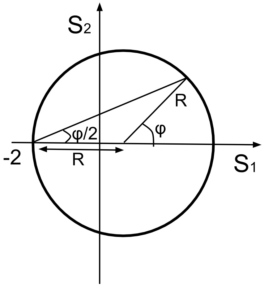
Figure 3: The geometry of Eq. (38) and Eq. (41). Note that $R$ may also be negative (then the center of the circle would be at $S_{1}<-2$).

We will proceed by using the Stokes variables defined as

$$\begin{split}&S_{0}=|\Omega_{1}|^{2}+|\Omega_{2}|^{2},\quad S_{3}=|\Omega_{1}|^{2}-|\Omega_{2}|^{2},\\ &S_{1}+iS_{2}=2\overline{\Omega}_{1}\Omega_{2}.\end{split}$$ (35)

The following result will prove central,

$$\frac{d}{dt}(S_{1}+iS_{2})=-\frac{i\,J}{4}\,M^{-}\,(S_{1}+2+iS_{2})^{2}.$$ (36)

If we define, $w=S_{1}+2+iS_{2}$, then Eq. (36) is

$$\frac{dw}{dt}=i\gamma\,w^{2}$$ (37)

where $\gamma$ is implicitly defined. This equation gives invariant circles $w\bar{w}-R(w+\bar{w})=0$, or

$$(S_{1}+2-R)^{2}+S_{2}^{2}=R^{2},$$ (38)

where $R\in\mathbb{R}$ is an arbitrary constant. Fig. 3 shows examples of these circles. Solving for $R$, we find that a conserved quantity is explicitly written as

$$\frac{(S_{1}+2)^{2}+S_{2}^{2}}{S_{1}+2}=2R.$$ (39)

Eq. (39) reproduces the result in Eq. (34). In order to see this, we write (34) in terms of the Stokes variables,

$$I_{1}=J\frac{(S_{1}+2)^{2}+S_{2}^{2}}{S_{1}^{2}+S_{2}^{2}-4}.$$ (40)

Both Eqs. (39) and (40) are quadratic in $S_{1},S_{2}$, and they give the same family of circles.

We conclude this subsection with some remarks. The point $S_{1}+iS_{2}=-2$ has a special role in this formulation, as it gives a fixed point of Eq. (36). It corresponds to $\overline{\Omega}_{1}\Omega_{2}=-1\Leftrightarrow\bm{m}_{1}=-\bm{m}_{2}$.

If we consider anisotropy $\kappa\neq 0$, the integral (33) does not represent simply a curve on the $(S_{1},S_{2})$ plane but a more complicated surface in the space $(S_{1},S_{2},S_{3})$.

A comparison of the results of the present section can be made with the more extensively studied system of two coupled nonlinear Schrödinger equations with cubic nonlinearity. The system has two conserved quantities that were reported in 2010_PRA_RamezaniKottos , and more extensively explained in Refs. 2013_PRA_BarashenkovJackson ; 2013_PRA_PicktonSusanto ; 2013_JPhys_KevrekidisPelinovsky . A calculation similar to that in Eq. (36) gives a form $dw/dt=i\gamma^{\prime}\,w$ with $\gamma^{\prime}$ some quantity independent of $w$; cf. Eq. (37). The solutions are a family of circles with the center at the origin of the plane $(S_{1},S_{2})$.

V.3 Exchange model, second integral

We write Eq. (38) in the parametric form

$$S_{1}+iS_{2}=R-2+Re^{i\phi},\qquad 0\leq\phi<2\pi,$$ (41)

whose geometric meaning is shown in Fig. 3. We substitute Eq. (41) in Eq. (36) and obtain

$$\frac{d}{dt}\left[\tan\left(\phi/2\right)\right]=\frac{R}{2}J\,M^{-}.$$ (42)

Eq. (42) gives the rate at which we move on a circle defined in Eq. (38). An example of the trajectory during the motion on the $(S_{1},S_{2})$ plane is shown in Fig. 4.

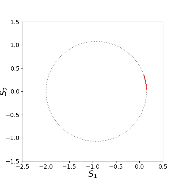
Figure 4: We simulate Eqs. (13) with parameters $J=1$ and $\beta=0.8$ (we set $\kappa=0,h=0$ and $\alpha=0$). The grey dotted line shows the circle (39) and the red arc shows the trajectory on the $(S_{1},S_{2})$ plane. All Stokes variables present oscillating motion in time (not shown).

We can now combine Eq. (42) with Eq. (29) and obtain a second conserved quantity

$$I_{2}=\tan\left(\phi/2\right)+\frac{R}{2}\frac{J}{\beta}\,\ln|M_{z}|.$$ (43)

In Fig. 3, we see that

$$\tan(\phi/2)=\frac{\sin\phi}{1+\cos\phi}=\frac{S_{2}}{S_{1}+2}.$$

and the conserved quantity (43) is written in terms of the Stokes variables as

$$I_{2}=\frac{S_{2}}{S_{1}+2}+\frac{R}{2}\frac{J}{\beta}\,\ln\left|2\frac{4-(S_{1}^{2}+S_{2}^{2})}{(S_{0}+2)^{2}-S_{3}^{2}}\right|$$ (44)

where we have used

$$M_{z}=2\frac{4-S_{0}^{2}+S_{3}^{2}}{(S_{0}+2)^{2}-S_{3}^{2}}=2\frac{4-(S_{1}^{2}+S_{2}^{2})}{(S_{0}+2)^{2}-S_{3}^{2}}.$$

The integral (44) could also be obtained by a combination of Eqs. (29) and (36). However, the method used in this subsection is a more transparent one as it is based on geometric arguments.

Finally, we note that if the system of equations could be produced by a Hamiltonian, the existence of the two integrals of motion would imply its complete integrability 2015_JPA_BarashenkovPelinovsky .

VI Concluding remarks

A system of interacting spins that are under spin transfer torque can be described by a complex function, or a non-Hermitian Hamiltonian. We give the formalism for obtaining the complex function that makes manifest the $\mathcal{PT}$ symmetry when this is present. We have studied the nonlinear dynamics dynamics and the exceptional point for a system of two exchange-coupled spins in a case of $\mathcal{PT}$ symmetry. This introduces a paradigm for the dynamics of non-Hermitian systems defined on the sphere.

We have identified the regime for periodic precessional motion of the two spins, and its stability. The periodic motion corresponds to a locking of the complete system in sustained magnetization oscillations. The synchronization of the oscillations of the two spins, due to $\mathcal{PT}$ symmetry, could lead to an answer to the long standing problem of the synchronization of spin-transfer torque nano-oscillators (STNO) 2017_NatPhys_AwadAkerman ; 2017_NatComms_LebrunCros . The rich spin dynamics for the spin system can be further used to study non-magnetic systems which are described by effective spin variables (e.g., as in polariton condensates 2020_NPJ_GhoshLiew ).

References

- (1) Ramy El-Ganainy, Konstantinos G. Makris, Mercedeh Khajavikhan, Ziad H. Musslimani, Stefan Rotter, and Demetrios N. Christodoulides. Non-Hermitian physics and PT symmetry. Nature Physics, 14(1):11–19, 2018.
- (2) Emil J. Bergholtz, Jan Carl Budich, and Flore K. Kunst. Exceptional topology of non-Hermitian systems. Rev. Mod. Phys., 93:015005, Feb 2021.
- (3) Vladimir V. Konotop, Jianke Yang, and Dmitry A. Zezyulin. Nonlinear waves in -symmetric systems. Rev. Mod. Phys., 88:035002, Jul 2016.
- (4) Mohammad-Ali Miri and Andrea Alù. Exceptional points in optics and photonics. Science, 363(6422):eaar7709, 2019.
- (5) Carl M Bender. Making sense of non-Hermitian Hamiltonians. Reports on Progress in Physics, 70(6):947–1018, may 2007.
- (6) Ingrid Rotter. A non-Hermitian Hamilton operator and the physics of open quantum systems. Journal of Physics A: Mathematical and Theoretical, 42(15):153001, mar 2009.
- (7) Carl M. Bender and Stefan Boettcher. Real spectra in non-Hermitian Hamiltonians having PT symmetry. Phys. Rev. Lett., 80:5243–5246, Jun 1998.
- (8) Christian E. Rüter, Konstantinos G. Makris, Ramy El-Ganainy, Demetrios N. Christodoulides, Mordechai Segev, and Detlef Kip. Observation of parity–time symmetry in optics. Nature Physics, 6(3):192–195, 2010.
- (9) Liang Feng, Zi Jing Wong, Ren-Min Ma, Yuan Wang, and Xiang Zhang. Single-mode laser by parity-time symmetry breaking. Science, 346(6212):972–975, 2014.
- (10) Alexey Galda and Valerii M. Vinokur. Parity-time symmetry breaking in magnetic systems. Phys. Rev. B, 94:020408, Jul 2016.
- (11) Alexey Galda and Valerii M. Vinokur. Linear dynamics of classical spin as Möbius transformation. Scientific Reports, 7(1):1168, 2017.
- (12) Alexey Galda and Valerii M. Vinokur. Exceptional points in classical spin dynamics. Scientific Reports, 9(1):17484, 2019.
- (13) I.V. Barashenkov and Alexander Chernyavsky. Stable solitons in a nearly PT-symmetric ferromagnet with spin-transfer torque. Physica D: Nonlinear Phenomena, 409:132481, 2020.
- (14) Huanhuan Yang, C. Wang, Tianlin Yu, Yunshan Cao, and Peng Yan. Antiferromagnetism emerging in a ferromagnet with gain. Phys. Rev. Lett., 121:197201, Nov 2018.
- (15) Xi-guang Wang, Guang-hua Guo, and Jamal Berakdar. Enhanced sensitivity at magnetic high-order exceptional points and topological energy transfer in magnonic planar waveguides. Phys. Rev. Applied, 15:034050, Mar 2021.
- (16) Steffen Wittrock, Salvatore Perna, Romain Lebrun, Roberta Dutra, Ricardo Ferreira, Paolo Bortolotti, Claudio Serpico, and Vincent Cros. Exceptional points controlling oscillation death in coupled spintronic nano-oscillators. arXiv:2108.04804, 2021.
- (17) Kuangyin Deng, Xin Li, and Benedetta Flebus. Exceptional points as a route to magnetic nano-oscillators. arXiv:2205.02308, 2022.
- (18) Haoliang Liu, Dali Sun, Chuang Zhang, Matthew Groesbeck, Ryan Mclaughlin, and Z. Valy Vardeny. Observation of exceptional points in magnonic parity-time symmetry devices. Science Advances, 5(11):eaax9144, 2019.
- (19) A. Hubert and R. Schäfer. Magnetic domains. Springer, Berlin, 1998.
- (20) Albert Fert, Nicolas Reyren, and Vincent Cros. Magnetic skyrmions: advances in physics and potential applications. Nature Reviews Materials, 2(7):17031, 2017.
- (21) Julie Grollier, Damien Querlioz, and Mark D. Stiles. Spintronic nanodevices for bioinspired computing. Proccedings of IEEE, 104:2024, 2016.
- (22) D.V. Berkov and J. Miltat. Spin-torque driven magnetization dynamics: Micromagnetic modeling. J. Magn. Magn. Mater., 320(7):1238–1259, 2008.
- (23) Stephen E Russek, William H Rippard, Thomas Cecil, and Ranko Heindl. Spin-Transfer Nano-Oscillators. In Handbook of Nanophysics, Handbook of Nanophysics, chapter 38, pages 1–23. CRC Press, Honolulu, USA, 2010.
- (24) A. A. Awad, P. Dürrenfeld, A. Houshang, M. Dvornik, E. Iacocca, R. K. Dumas, and J. Åkerman. Long-range mutual synchronization of spin hall nano-oscillators. Nature Physics, 13(3):292–299, 2017.
- (25) R. Lebrun, S. Tsunegi, P. Bortolotti, H. Kubota, A. S. Jenkins, M. Romera, K. Yakushiji, A. Fukushima, J. Grollier, S. Yuasa, and V. Cros. Mutual synchronization of spin torque nano-oscillators through a long-range and tunable electrical coupling scheme. Nature Communications, 8(1):15825, 2017.
- (26) Yang Wu, Wenquan Liu, Jianpei Geng, Xingrui Song, Xiangyu Ye, Chang-Kui Duan, Xing Rong, and Jiangfeng Du. Observation of parity–time symmetry breaking in a single-spin system. Science, 364:878, 2019.
- (27) Sanjib Ghosh and Timothy C. H. Liew. Quantum computing with exciton-polariton condensates. npj Quantum Information, 6:16, 2020.
- (28) William Legrand, Davide Maccariello, Fernando Ajejas, Sophie Collin, Aymeric Vecchiola, Karim Bouzehouane, Nicolas Reyren, Vincent Cros, and Albert Fert. Room-temperature stabilization of antiferromagnetic skyrmions in synthetic antiferromagnets. Nature Materials, 19(1):34–42, 2020.
- (29) Yu. B. Gaididei, unpublished.
- (30) A. Bose and D. C. Ralph. Tilted spin current generated by an antiferromagnet. Nature Electronics, 5, 2022.
- (31) Arnab Bose, Nathaniel J. Schreiber, Rakshit Jain, Ding-Fu Shao, Hari P. Nair, Jiaxin Sun, Xiyue S. Zhang, David A. Muller, Evgeny Y. Tsymbal, Darrell G. Schlom, and Daniel C. Ralph. Tilted spin current generated by the collinear antiferromagnet ruthenium dioxide. Nature Electronics, 5, 2022.
- (32) J. M. Lee, T. Kottos, and B. Shapiro. Macroscopic magnetic structures with balanced gain and loss. Phys. Rev. B, 91:094416, Mar 2015.
- (33) Hilary M. Hurst and Benedetta Flebus. Perspective: non-hermitian physics in magnetic systems. arXiv:2209.03946, 2022.
- (34) Ali Mostafazadeh. Exact PT-symmetry is equivalent to hermiticity. J. Phys. A: Math. Gen., 36:2081, 2003.
- (35) I. V. Barashenkov. Hamiltonian formulation of the standard PT-symmetric nonlinear schrödinger dimer. Phys. Rev. A, 90:045802, Oct 2014.
- (36) I V Barashenkov and Mariagiovanna Gianfreda. An exactly solvable PT-symmetric dimer from a Hamiltonian system of nonlinear oscillators with gain and loss. Journal of Physics A: Mathematical and Theoretical, 47(28):282001, jun 2014.
- (37) I V Barashenkov, D E Pelinovsky, and P Dubard. Dimer with gain and loss: Integrability and PT-symmetry restoration. Journal of Physics A: Mathematical and Theoretical, 48(32):325201, jul 2015.
- (38) Hamidreza Ramezani, Tsampikos Kottos, Ramy El-Ganainy, and Demetrios N. Christodoulides. Unidirectional nonlinear -symmetric optical structures. Phys. Rev. A, 82:043803, Oct 2010.
- (39) I. V. Barashenkov, G. S. Jackson, and S. Flach. Blow-up regimes in the -symmetric coupler and the actively coupled dimer. Phys. Rev. A, 88:053817, Nov 2013.
- (40) J. Pickton and H. Susanto. Integrability of -symmetric dimers. Phys. Rev. A, 88:063840, Dec 2013.
- (41) Panayotis G Kevrekidis, Dmitry E Pelinovsky, and Dmitry Y Tyugin. Nonlinear dynamics in PT-symmetric lattices. J. Phys. A: Math. Theor., 46(36):365201, 2013.