Nuclear masses and the equation of state of nuclear matter

Abstract

The incompressible liquid-drop (ILD) model reproduces masses of stable nuclei rather well. Here we show how the ILD volume, surface, symmetry, and Coulomb energies are related to the equation of state of nuclear matter using the Oyamatsu-Iida (OI) macroscopic nuclear model, which has reasonable many-body energy and isoscalar inhomogeneity gradient energy. We use 304 update interactions, covering wide ranges of the incompressibility $K_{0}$ of symmetric matter and the density slope of symmetry energy $L$, which fit almost equally empirical mass and radius data of stable nuclei. Thus, the $K_{0}$ and $L$ dependences are nearly frozen in stable nuclei as in the ILD model, leading to clear correlations among interaction and saturation parameters. Furthermore, we assume that the surface energy of the OI model is twice as large as the gradient energy using the size equilibrium conditions of the ILD and OI models. Then, the four energies of the ILD and OI models agree well for stable nuclei with $A\gtrsim 40$. Meanwhile, the OI model with $L\lesssim 100$ MeV predicts the latest mass data better than those of stable nuclei, and we suggest $20\lesssim L\lesssim 90$ MeV, although the lower boundary is not constrained well.

xxxx, xxx

1 Introduction

The incompressible liquid drop (ILD) model, also referred to as the Weizsäcker-Bethe mass formula, assumes the same sharp nuclear surface for the neutron and proton distributions and fits rather well the observed masses and neutron excesses of the $\beta$-stable nuclei BohrMottelson1968 . Meanwhile, the observed radii can also be reproduced well in the macroscopic nuclear model using the equation of state (EOS) of uniform nuclear matter and appropriate inhomogeneity energy correction due to finite-range effects of nuclear forces Lombard1973 .

The Oyamatsu-Iida (OI) macroscopic nuclear model OI2003 for studies on laboratory nuclei and neutron star matter OI2007 ; Oyamatsu:2010bf ; Oyamatsu:2010sk ; Iida:2013fra ; Sotani:2013dga ; Sotani:2012qc ; Sotani:2012xd ; Sotani:2013jya ; Sotani:2015lya ; Sotani:2015laa ; Sotani:2016pmb ; Sotani:2017hpq ; Sotani:2018tdr ; Sotani:2019pja is one of the latter type models. It is essentially based on the assumption of the density functional theory (DFT), initially developed for interacting electrons, which states the total energy can be written as a functional of the local density Hohenberg:1964zz ; Kohn:1965zza . The introduction section of Ref. Lombard1973 gives a concise discussion of macroscopic nuclear models at the dawn of the DFT.

The OI model has three distinct features from other macroscopic models using phenomenological nuclear interactions, such as the Skyrme Hartree-Fock theory and relativistic mean field theory (see, for example, Ref. BrackGuetHakansson1985 for a review of microscopic and macroscopic descriptions using Skyrme interactions). First, the OI model parameterizes the EOS and inhomogeneity energy directly, although it loses the direct connection between nuclear forces and the EOS. Special attention is paid to the incompressibility $K_{0}$ and the slope of symmetry energy $L$ of the EOS because the nuclear structure is determined from the local pressure equilibrium. Second, the OI model is designed as a compressible liquid drop model allowing the independent radius and surface diffuseness parameters for the neutron and proton distributions. Third, to smooth out the shell effects, the interaction parameters of the OI model are fitted to the smoothed empirical mass and radius data of stable nuclei rather than the experimental data. These smoothed data MYamada1964 were evaluated from the systematics YamadaMatumoto1961JPSJ , and eventually, the neutron excess values take decimal values rather than integers.

The OI model has been used to study unstable nuclei and neutron star matter OI2007 ; Oyamatsu:2010bf ; Oyamatsu:2010sk ; Iida:2013fra ; Sotani:2013dga ; Sotani:2012qc ; Sotani:2012xd ; Sotani:2013jya ; Sotani:2015lya ; Sotani:2015laa ; Sotani:2016pmb ; Sotani:2017hpq ; Sotani:2018tdr ; Sotani:2019pja . Therefore, it is time to summarize the results of these studies and clarify how the EOS of nuclear matter affects the structures of the laboratory nuclei and neutron star matter. In this paper, we reexamine how many EOS saturation parameters are constrained by the empirical mass and radius data of stable nuclei. Then, we show that masses of unstable nuclei correlate with the $L$ value and compare this correlation with the recently reported $L$ values evaluated from ²⁰⁸Pb neutron skin and Sn+Sn experiments Reed:2021nqk ; Reinhard:2021utv ; SRIT:2021gcy . Furthermore, we discuss how the EOS and the inhomogeneity energy are related to the ILD volume, surface, symmetry, and Coulomb energies, showing that the OI model has two more degrees of freedom of $K_{0}$ and $L$ than the ILD model. We will also take a look at the surface diffuseness in the most stable nuclei because the nuclear density distributions are not yet satisfactory in the macroscopic nuclear model Lombard1973 . In future papers, we plan to discuss the neutron drip and neutron star matter based on the results of this paper.

This paper is arranged as follows. Section 2 describes the OI model in detail. Section 2.1 defines uniform matter energy, density-dependent symmetry energy, and saturation parameters. Section 2.2 describes a nucleus in the OI model. In Sec. 2.3, we update the values of the interaction parameters and show to what extent the updated interactions fit the empirical data of stable nuclei. Section 3 shows the obtained correlations among the interaction and saturation parameters and gives the numerical results of nuclear mass calculations. Section 4 shows how the volume, surface, and symmetry energies of the ILD model are represented in the OI model. Finally, the conclusions of this paper are given in Sec. 5.

2 Oyamatsu-Iida macroscopic nuclear model

The Oyamatsu-Iida (OI) macroscopic nuclear model OI2003 is an update of model IV for the early study of pasta nuclei in the neutron-star crust oya1993 . The OI model has the following three important features compared to the ILD model.

• Nuclear energy in a nucleus is the integral of the local uniform-matter and inhomogeneity energy densities.

• The inhomogeneity energy density is proportional to the square of the gradient of the local nucleon density.

• The neutron and proton distributions are independent; each distribution is parameterized with radius and diffuseness parameters.

2.1 Uniform-matter energy density $\epsilon_{0}\left(n_{n},n_{p}\right)$

We write the energy density $\epsilon_{0}\left(n_{n},n_{p}\right)$ of uniform nuclear matter as the sum of the free kinetic energy density and the potential energy density. The potential energy density is the weighted sum of $v_{s}(n)$ for symmetric matter and $v_{n}(n)$ for neutron matter.

$$\epsilon_{0}\left(n_{n},n_{p}\right)=\frac{3}{5}(3\pi^{2})^{2/3}\left(\frac{\hbar^{2}}{2m_{n}}n_{n}^{5/3}+\frac{\hbar^{2}}{2m_{p}}n_{p}^{5/3}\right)+(1-\alpha^{2})v_{s}(n)+\alpha^{2}v_{n}(n)$$ (1)

with $\alpha=(n_{n}-n_{p})/n$. These potential energy densities are parametrized as

$$v_{s}(n)=a_{1}n^{2}+\frac{a_{2}n^{3}}{1+a_{3}n},\quad v_{n}(n)=b_{1}n^{2}+\frac{b_{2}n^{3}}{1+b_{3}n}.$$ (2)

The coefficients $a_{1}\ (b_{1})$ and $a_{2}\ (b_{2})$ are two- and three-body energy coefficients for symmetric (neutron) matter, respectively. The coefficients $a_{3}$ and $b_{3}$ are the many-body parameters that control the strength of many-body ($N\geq 4$) energies. For example, the potential energy density $v_{s}(n)$ can be expanded as

$$v_{s}(n)=a_{1}n^{2}+a_{2}n^{3}[1-a_{3}n+(a_{3}n)^{2}-(a_{3}n)^{3}+\cdots].$$ (3)

Here, the two-body, three-body, and $N-$body ($N\geq 4$) energy densities are $a_{1}n^{2}$, $a_{2}n^{3}$, and $a_{2}n^{3}(-a_{3}n)^{N-3}$, respectively. The potential energy density of the form in Eq. (2) was proposed by Buldman and DoverBludmanDover1980 to make the equation of state soft and causal at high densities. It can fit the popular nuclear matter EOS by Friedman and Pandharipande (FP) FriedmanPandharipande1980 up to $n=0.3$ (fm^-3) oya1993 . However, it is challenging to constrain the many-body parameter $b_{3}$ of neutron matter from stable nuclei. Therefore, we set $b_{3}$ = 1.58632 fm³ oya1993 ; OI2003 , chosen to fit the FP neutron matter EOS FriedmanPandharipande1980 to give reasonable many-body energy for neutron matter. As a side note, $v_{n}(n)$ in the early studyoya1993 has an additional constraint $b_{1}/b_{2}=-0.3232$ to fit the FP neutron matter EOS better.

It is convenient to consider the energy per nucleon of the matter as a function of the total nucleon density $n$ and the neutron excess $\alpha=(n_{n}-n_{p})/n$. This energy per nucleon

$$w(n,\alpha)=\epsilon_{0}(n_{n},n_{p})/n$$ (4)

is often referred to as the equation of state (EOS).

Saturation parameters are essentially the density derivative coefficients of $w(n,\alpha)$ at the saturation ($n=n_{0}$ and $\alpha=0$); thereby, the behavior of the EOS close to the saturation is determined mainly by low order saturation parameters. We write the energies of symmetric nuclear matter ($\alpha=0$) and neutron matter ($\alpha=1$) as $w_{s}(n)=w(n,0)$ and $w_{n}(n)=w(n,1)$, respectively. Due to the charge symmetry property of the nuclear interaction, $w(n,\alpha)$ can be expanded into the Taylor series with respect to $\alpha^{2}$:

$$w(n,\alpha)=w_{s}(n)+S^{(2)}(n)\alpha^{2}+\frac{1}{2}S^{(4)}(n)\alpha^{4}+\frac{1}{6}S^{(6)}(n)\alpha^{6}+\cdots,$$ (5)

with

$$S^{(2k)}(n)=\frac{\partial^{k}w}{\partial(\alpha^{2})^{k}}\Big{|}_{\alpha=0}\quad(k=1,2,\cdots).$$ (6)

The energy $S^{(2)}(n)$ dominates the asymmetry energy and is usually referred to as the density-dependent symmetry energy $S(n)$.

It is useful to expand the three energies $w_{s}(n)$, $w_{n}(n)$, and $S(n)$ in the neighborhood of the saturation density $n=n_{0}$ using a dimensionless parameter $\displaystyle u=\frac{n-n_{0}}{3n_{0}}$ instead of $n$.

$$w_{s}(n)=w_{0}+L_{0}u+\frac{1}{2}K_{0}u^{2}+\frac{1}{6}Q_{0}u^{3}+\cdots,$$ (7)

$$w_{n}(n)=w_{n0}+L_{n0}u+\frac{1}{2}K_{n0}u^{2}+\frac{1}{6}Q_{n0}u^{3}+\cdots,$$ (8)

$$S(n)=S_{0}+Lu+\frac{1}{2}K_{sym}u^{2}+\frac{1}{6}Q_{sym}u^{3}+\cdots,$$ (9)

The coefficients in Eqs. (7)-(9) are called saturation parameters. In Eq. (7), the density slope $L_{0}$ is zero from the saturation condition.

This paper only discusses the saturation parameters up to $Q_{0}$, $Q_{n0}$, and $Q_{sym}$. These $Q$s in Eqs. (7)-(9) are proportional to the third-order derivative coefficients of density and depend only on the three-body and many-body parameters ($a_{2},a_{3},b_{2}$, and $b_{3}$) in the OI model. The explicit formula giving relations between the potential parameters ($a_{1}-a_{3},\ b_{1}-b_{3}$) and the low order saturation parameters are given in Appendix A.

In addition to the saturation parameters in Eqs. (7)-(9), we introduce auxiliary parameter $y$, the density slope of the saturation curve at $\alpha=0$, to reasonably constrain isovector interaction. In the lowest-order approximation,

$$y=-\frac{S_{0}K_{0}}{3n_{0}L}.$$ (10)

2.2 Nucleus described in the OI model

The mass excess, $M_{ex}$, of a charge-neutral atomic nucleus of proton number $Z$, neutron number $N$, and mass number $A=N+Z$ is the sum of the EOS (uniform-matter) energy $W_{EOS}$, the gradient (inhomogeneity) energy $W_{g}$, the Coulomb energy $W_{C}$, and the rest mass energy $\Delta m$.

$$M_{ex}=W_{EOS}+W_{g}+W_{c}+\Delta m,$$ (11)

$$\Delta m=m_{n}N+(m_{p}+m_{e})Z-m_{u}A$$ (12)

with the neutron mass $m_{n}$, the proton mass $m_{p}$, the electron mass $m_{e}$, and the atomic mass unit $m_{u}$. In Eq. (12), we use $m_{p}+m_{e}$ instead of the hydrogen mass $m_{H}$. The difference between $m_{p}+m_{e}$ and $m_{H}$ is numerically minor, less than one keV. This use of the electron rest mass $m_{e}$ is helpful in the neutron-star matter calculation because the electron energy of the neutron-star matter is approximated well by the relativistic electron kinetic energy oya1993 ; OI2007 .

The neutron number $N$ (proton number $Z$) is given by the integral of local neutron (proton) number density $n_{n}(r)$ ($n_{p}(r)$).

$$N=\int d^{3}r\ n_{n}(r),$$ (13)

$$Z=\int d^{3}r\ n_{p}(r).$$ (14)

The mass number $A$ is given by

$$A=\int d^{3}r\ (n_{n}(r)+n_{p}(r))=\int d^{3}r\ n(r)$$ (15)

with the total nucleon number density $n(r)=n_{n}(r)+n_{p}(r)$.

As in our previous studies OI2003 ; OI2007 ; Oyamatsu:2010bf ; Oyamatsu:2010sk ; Iida:2013fra ; Sotani:2013dga ; Sotani:2012qc ; Sotani:2012xd ; Sotani:2013jya ; Sotani:2015lya ; Sotani:2015laa ; Sotani:2016pmb ; Sotani:2017hpq ; Sotani:2018tdr ; Sotani:2019pja , we assume that the local nuclear energy density is the sum of the uniform-matter energy density $\epsilon_{0}(n_{n},n_{p})$ and the gradient energy density $F_{0}|\nabla n(r)|^{2}$ with constant $F_{0}$. The EOS energy is

$$W_{EOS}=\int d^{3}r\ \epsilon_{0}\left(n_{n}(r),n_{p}(r)\right),$$ (16)

and the gradient energy is

$$W_{g}=\int d^{3}r\ F_{0}|\nabla n(r)|^{2}.$$ (17)

Note that the surface energy comes from both $W_{EOS}$ and $W_{g}$. See Appendix C for the other choices of the inhomogeneity energy densities used in our early study of neutron star matteroya1993 .

The Coulomb energy is given by

$$W_{C}=\frac{e^{2}}{2}\int d^{3}rd^{3}r^{\prime}\frac{n_{p}(r)n_{p}(r^{\prime})}{|r-r^{\prime}|}$$ (18)

with the electron charge $e$.

The OI model is a compressible liquid drop model capable of independently choosing radii and surface thicknesses for the neutron and proton distributions. We consider the point nucleon distribution $n_{i}(r)\ (i=n,p)$ as a parametrized function of the distance $r$ from the center with edge radius parameter $R_{i}$ and relative surface diffuseness parameter $t_{i}$;

$$n_{i}(r)=\begin{cases}n_{i}^{in}\left(1-\left(\frac{r}{R_{i}}\right)^{t_{i}}\right)^{3}\qquad\qquad\qquad(r\leq R_{i})\\ 0\qquad\qquad\qquad\qquad\qquad\qquad(r\geq R_{i}),\end{cases}$$ (19)

where $n_{i}^{in}$ is the central density. The density at $r\geq R_{i}$ is zero because the nucleon density outside the classical turning point is zero.

For given $Z$ and $A$, the values of the distribution parameters, $n_{i}^{in}$, $R_{i}$, and $t_{i}$, are chosen to minimize the mass excess calculated from Eqs. (11)–(18). Equation (19) enables us to calculate the gradient energy $W_{g}$ and the Coulomb energy $W_{C}$ analytically.

The root-mean-square (rms) radius of the charge distribution is given by

$$R_{ch}=\sqrt{\frac{1}{Z}\int d^{3}r\ r^{2}\int d^{3}r^{\prime}\ n_{p}(\bf{r^{\prime}})\rho(|\bf{r}-\bf{r}^{\prime}|)},$$ (20)

using the proton charge form factor EltonSwift67 ;

$$\rho(r)=\left(\frac{1}{\sqrt{\pi}a_{p}}\right)^{3}\exp\left[-(r/a_{p})^{2}\right],$$ (21)

with $a_{p}=0.65$ (fm). The rms radii of the proton and neutron distributions, $R_{rms\_p}(=R_{ch})$ and $R_{rms\_n}$, are also calculated in the same way using the form factor $\rho(r)$. Then, the rms radius of the matter distribution, $R_{m}$, is given by

$$R_{m}=\sqrt{\frac{N\ R_{rms\_n}^{2}+Z\ R_{rms\_p}^{2}}{A}}.$$ (22)

The definition of surface thickness is not unique. The 90%-10% surface thickness is the distance between the surfaces where the density is 90% and where it is 10% of the central density. For the point nucleon distribution (19), the 90%-10% surface thickness is given by

$$\textrm{thick}(i)=R_{i}\left[(1-0.1^{1/3})^{1/t_{i}}-(1-0.9^{1/3})^{1/t_{i}}\right]\quad(i=n,p).$$ (23)

We will use this quantity (23) to discuss the point nucleon distributions of the most stable nucleus in Sec. 4.3.

2.3 Optimization of interaction parameters

The values of the five potential parameters $a_{1}-a_{3}$ and $b_{1}-b_{2}$, and the inhomogeneity parameter $F_{0}$ are optimized to fit the smoothed empirical data of neutron excess $I$, mass excess $M_{ex}$, and rms charge radius $R_{ch}$ of stable nuclei in Table 1. In his early mass formula study MYamada1964 , Yamada evaluated the smoothed values of $I$ and $M_{ex}$ for the nine mass numbers based on the systematics of the neutron and proton separation energies YamadaMatumoto1961JPSJ to represent the average trends of the $\beta$-stable nuclei. Note that the fractional $I$ values are allowed in Table 1. Meanwhile, the present author evaluated the $R_{ch}^{emp}$ values oya1993 from the rms charge radius data in Ref. 1987ChargeRadii . The empirical data in Table 1 were used in our previous work OI2003 and our early neutron star matter study oya1993 .

The optimization using the smoothed empirical data in Table 1 gives an alternative way to obtain the EOS, presumably comparable to fitting the latest experimental mass data of all stable nuclei using a phenomenological nuclear interaction. Numerically, the experimental data of $I$ and $M_{ex}$ for $\beta$-stable nuclei were known at the time of the evaluation in Ref. MYamada1964 with sufficient accuracy YamadaMatumoto1961JPSJ ; 1961NuclidicMassTable . We also mention that deriving the macroscopic nuclear properties requires a certain smoothing or averaging, equivalent to evaluating the shell effects, which is more or less uncertain and dependent on phenomenological interactions.

The following empirical constraints are also imposed to limit the parameter space reasonablyoya1993 ; OI2003 :

• many-body energy parameter of neutron matter ($b_{3}=1.58632\ (\mathrm{fm}^{3})$),

• incompressibility of symmetric matter ($K_{0}=180,190,\cdots,360(\mathrm{MeV})$, 19 values),

• slope of saturation curve at $\alpha=0$ ($-y=200,210,\cdots,1800\ (\mathrm{MeV\cdot fm^{3}})$, 16 values).

In the present update, $-y=210,230,270(\mathrm{MeV\cdot fm^{3}})$ are added to the previous version OI2003 so that the present update has 304$(=16\times 19)$ interactions while the earlier version has 247$(=13\times 19)$ OI2003 .

Table 1: The empirical values of the neutron excess $I^{emp}$, mass excess $M_{ex}^{emp}$ and rms charge radius $R_{ch}^{emp}$ as functions of mass number $A$ on the smoothed $\beta$ stability line.oya1993 ; OI2003

$A$	$I^{emp}$	$M_{ex}^{emp}$ (MeV)	$R_{ch}^{emp}$ (fm)
25	0.18	-13.10	3.029
47	3.29	-46.17	3.567
71	7.61	-72.38	3.997
105	14.83	-89.69	4.487
137	22.71	-84.89	4.874
169	31.31	-61.18	5.206
199	39.78	-23.12	5.466
225	46.64	21.22	–
245	52.22	61.21	–

For a given $(y,K_{0})$, the values of the four parameters $n_{0},w_{0},S_{0}$, and $F_{0}$ are chosen to fit the empirical data in Table 1. We can easily judge whether or not the numerical optimization result is physical from the saturation parameter values. Then, the interaction parameters, $a_{1}-a_{3}$ and $b_{1}-b_{2}$, are calculated from $y,K_{0},n_{0},w_{0}$, and $S_{0}$. Eventually, we can calculate any saturation parameter from $a_{1}-a_{3}$ and $b_{1}-b_{3}$.

Specifically, we minimize

$$\chi^{2}=\sum\Big{[}\Big{(}\frac{I^{cal}-I^{emp}}{\Delta I}\Big{)}^{2}+\Big{(}\frac{M_{ex}^{cal}-M_{ex}^{emp}}{\Delta M}\Big{)}^{2}+\Big{(}\frac{R_{ch}^{cal}-R_{ch}^{emp}}{\Delta R}\Big{)}^{2}\Big{]},$$ (24)

with $\Delta I=0.1,\ \Delta M=1$ (MeV) and $\Delta R=0.01$ (fm). This optimization is not easy because we first calculate (optimize) the most stable isobars for the nine mass numbers in Table 1 and then optimize the $\chi^{2}$ value in Eq. (24). In the present update, the initial values of the parameters are chosen to make the optimum parameter values vary smoothly as functions of $(y,K_{0})$.

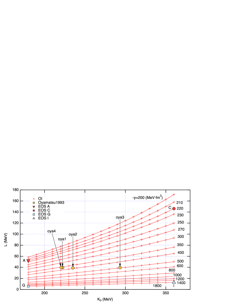
Figure 1: The plots of $(K_{0},L)$ for the present 304 interactions. The value of the slope $y$ is attached to the line joining the points with the same $y$ value. Also plotted are the four models oya1-4 in our early neutron star matter study oya1993 and the four extreme EOSs A, C, G, and I defined in our previous study OI2003 (see also Table 2).

Table 2: The values of saturation parameters of four models I-IV (oya1-4) in our early study of neutron-star matter oya1993 , together with the present update values of four extreme EOSs (A, C, G, and I) defined in Ref. OI2003 . The $S_{0}$ values are calculated using Eq. (54). Note that the inhomogeneity energy of oya1-3 and the definition of $S_{0}$ were different in the early studyoya1993 (see Appendix C).

EOS	$-y$	$K_{0}$	$L$	$n_{0}$	$w_{0}$	$S_{0}$	$F_{0}$
	(MeV $\cdot$ fm3)	(MeV)	(MeV)	(fm-3)	(MeV)	(MeV)	(MeV $\cdot$ fm5)
oya1	359.93	222.41	39.559	0.15856	-16.076	30.452	47.399
oya2	411.63	235.14	39.010	0.15227	-16.013	31.195	49.522
oya3	479.15	293.36	39.513	0.15845	-16.312	30.678	47.294
oya4	359.27	220.76	39.743	0.15807	-16.070	30.671	68.650
A	220	180	52.266	0.16921	-16.252	32.427	71.360
C	220	360	146.16	0.14578	-16.119	39.065	66.985
G	1800	180	5.6552	0.16864	-16.189	28.611	69.856
I	1800	360	12.789	0.14896	-16.031	28.575	61.660

Figure 1 plots the $(K_{0},L)$ values for the 304 interactions (EOSs) and shows lines joining the points with the same $y$ value for the eye guide. The $L$ value is calculated from Eq. (10) using $y,n_{0},S_{0}$, and $K_{0}$. This figure shows the one-to-one correspondence between $(K_{0},y)$ and $(K_{0},L)$. Hereafter, we take $L$ as an independent parameter instead of $y$ and analyze the interaction and saturation parameters as functions of $(K_{0},L)$. Figure 1 also depicts the four models oya1-4 of our early neutron-star matter studyoya1993 and four extreme EOSs A, C, G, and I defined in our previous work OI2003 , whose values of saturation parameters are listed in Table 2. The neutron matter EOSs of oya1-4 have only one free potential parameter because the study fixed the $b_{1}/b_{2}$ value. This constraint leads to $L\approx 40$ MeV, close to the FP EOS fit oya1993 .

Figure 2 plots the optimum $\chi^{2}$ values for the present 304 interactions and the previous 247 interactions OI2003 . The range of $\chi^{2}$ is relatively narrow, and $\chi^{2}$ is minimum at $K_{0}=220$ MeV and $L$=16.580 MeV. The present optimization reasonably minimizes the $\chi^{2}$ value and improves the overall optimization results compared with the previous work OI2003 . Meanwhile, the previous version shows insufficient minimizations and overfitting at $K_{0}=290$ (MeV) and $L\approx 69$ (MeV). These kinds of numerical uncertainty are inevitable even in the present update. To overcome these difficulties, we take many data points and focus on gross behavior as a function of $(K_{0},L)$ in our studies OI2003 ; OI2007 ; Oyamatsu:2010bf ; Oyamatsu:2010sk ; Iida:2013fra ; Sotani:2012qc ; Sotani:2012xd ; Sotani:2013jya ; Sotani:2013dga ; Sotani:2015lya ; Sotani:2015laa ; Sotani:2016pmb ; Sotani:2017hpq ; Sotani:2018tdr ; Sotani:2019pja .

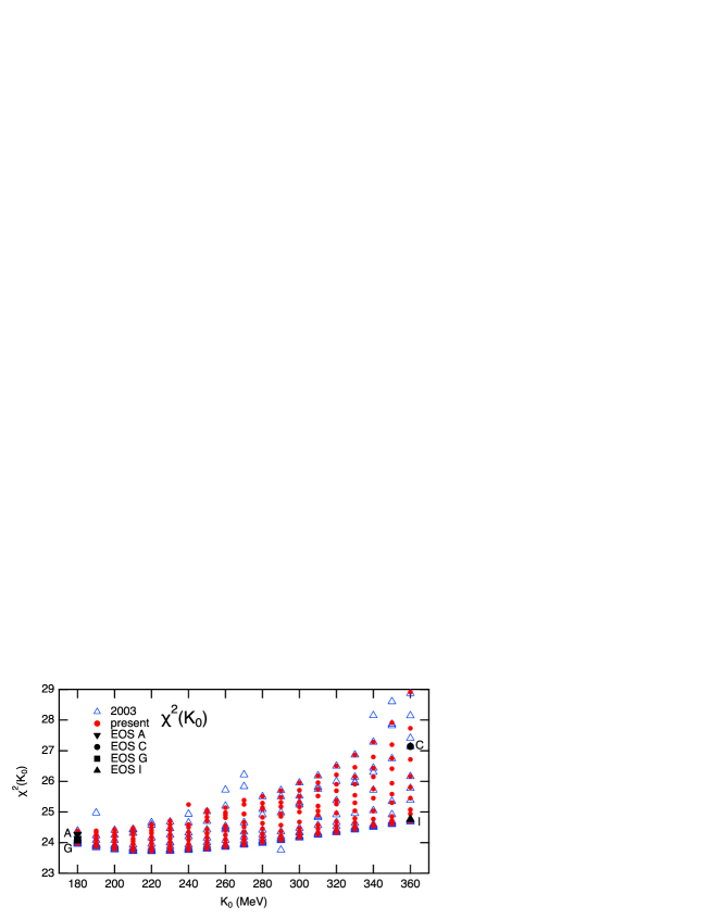
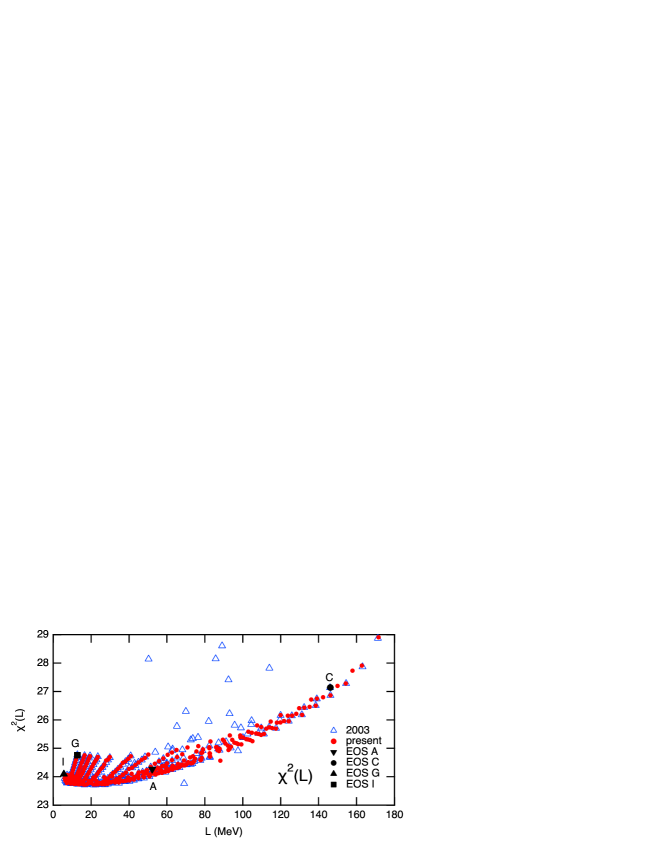
Figure 2: The $\chi^{2}$ values of the present update (filled red circles) and the previous 2003 study (open triangles) OI2003 as functions of $K_{0}$ and $L$. Also plotted are EOSs A, C, G, and I OI2003 in Table 2.

To examine the significant contribution to the optimum $\chi^{2}$, Fig. 3 shows the rms deviations of neutron excess $I$, mass excess $M_{ex}$, and charge radius $R_{ch}$ from the empirical values in Table 1. Their correlations with $K_{0}$ and $L$ are seen more clearly in the present study. From Eq. (24) and Fig. 3, we see that the dominant contribution to $\chi^{2}$ comes from neutron excess $I$. The rms deviation of neutron excess $I$ mainly correlates with $L$ and has appreciable sensitivity with $K_{0}$, while that of mass excess $M_{ex}$ strongly correlates with $L$. Meanwhile, the rms deviation of charge radius $R_{ch}$ strongly correlates with $K_{0}$ below 280 (MeV); above this $K_{0}$ value, its sensitivity to $L$ increases with $K_{0}$. It is also noted that the overfitting of $\chi^{2}$ in Fig. 2 at $K_{0}=290$ (MeV) and $L\approx 69$ (MeV) stems from the overfitting of neutron excess $I$ in Fig. 3.

It is remarked that the present 304 interactions fit the empirical values of $I^{emp}$, $M_{ex}^{emp}$, and $R_{ch}^{emp}$ almost equally in the sense that the deviations from the empirical values are much smaller than the fluctuations due to the shell effects, as shown in Fig. 17 in Appendix B. Thus, the $K_{0}$ and $L$ degrees of freedom are nearly frozen for $I$, $M_{ex}$, and $R_{ch}$ of stable nuclei. We will confirm this insensitivity for $M_{ex}$ in Sec. 3.5.

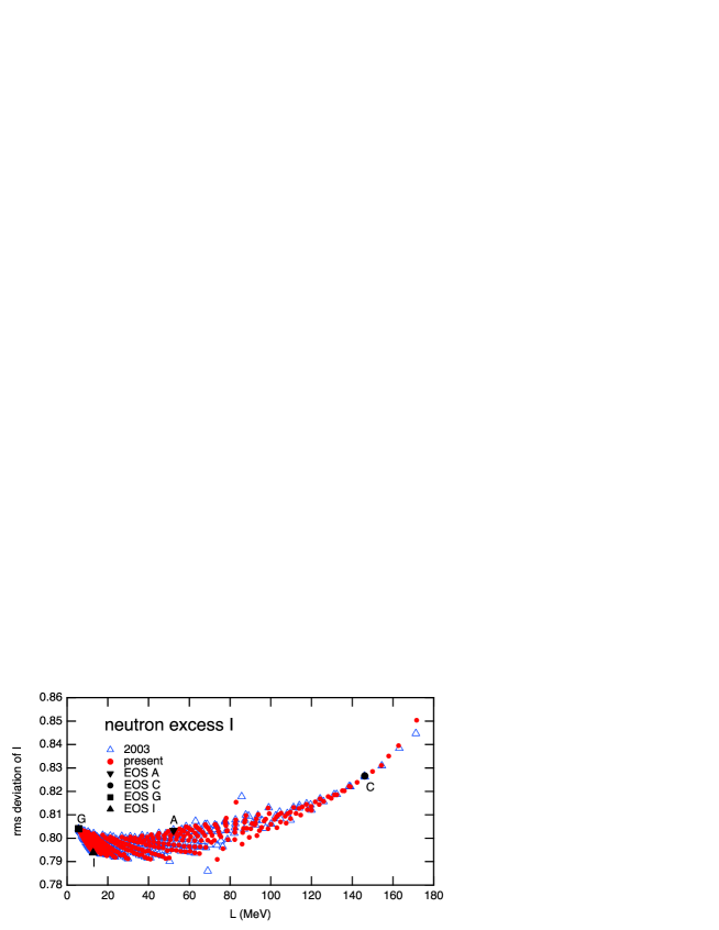
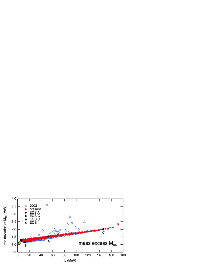
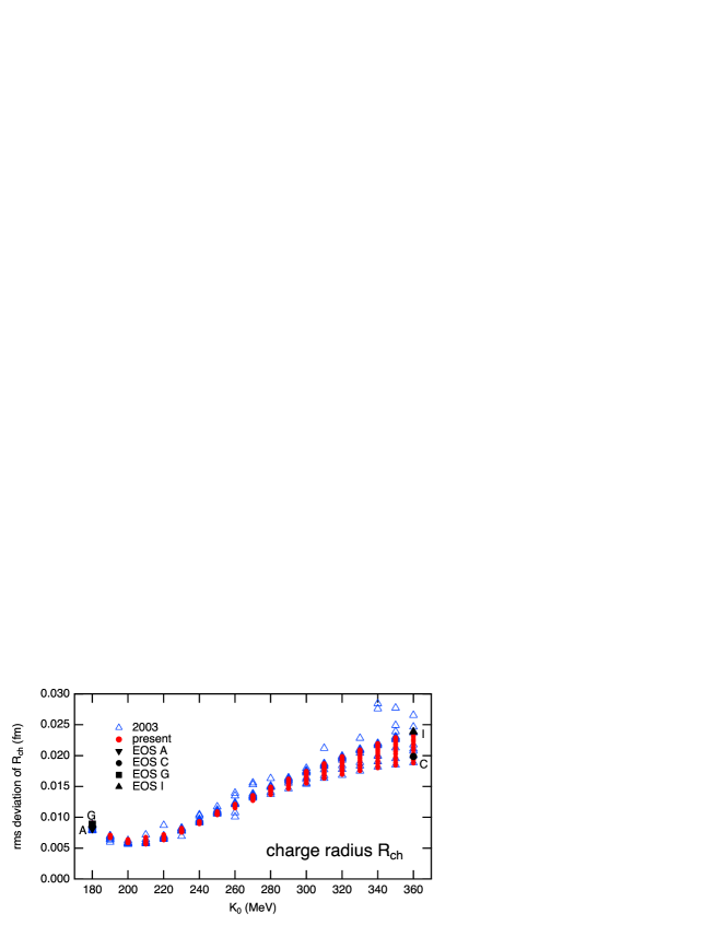
Figure 3: The rms deviations of neutron excess $I$, mass excess $M_{ex}$, and charge radius $R_{ch}$ from the smoothed empirical values in Table 1. The symbols are the same as those in Fig. 2.

3 Numerical results

3.1 Optimum values of potential parameters and their correlations

The symmetric matter potential, $v_{s}(n)$, essentially has only one degree of freedom. Figure 4 shows, in the upper panels, strong correlations among the potential parameters $a_{1}-a_{3}$ and the incompressibility $K_{0}$. The potential parameters $a_{1}-a_{3}$ show clear dependences on $K_{0}$. The lower panels show that the two-body energy coefficient $a_{1}$ and the many-body parameter $a_{3}$ strongly correlate with the three-body energy coefficient $a_{2}$. Consequently, the symmetric matter EOS $w_{s}(n)$ depends on $K_{0}$ and the three-body energy coefficient $a_{2}$.

Similarly, the neutron matter potential, $v_{n}(n)$, essentially has only one degree of freedom. Figure 5 shows that, in the upper panel, the potential parameters $b_{1}$ and $b_{2}$ have clear dependences on $L$ while, in the lower panel, the two-body energy coefficient $b_{1}$ also correlates strongly with the three-body energy coefficient $b_{2}$. Consequently, the neutron matter EOS $v_{n}(n)$ depends on $L$ and the three-body energy coefficient $b_{2}$.

It is also noteworthy in Figs. 4 and 5 that the two-body coefficients ($a_{1},b_{1}$) are constrained much better than the three-body coefficients ($a_{2},b_{2}$) and the many-body coefficient $a_{3}$. Meanwhile, the $b_{3}$ value, relevant to the high-density EOS, is so uncertain that we fix the value in our studies oya1993 ; OI2003 ; OI2007 ; Oyamatsu:2010bf ; Oyamatsu:2010sk ; Iida:2013fra ; Sotani:2013dga ; Sotani:2012qc ; Sotani:2012xd ; Sotani:2013jya ; Sotani:2015lya ; Sotani:2015laa ; Sotani:2016pmb ; Sotani:2017hpq ; Sotani:2018tdr ; Sotani:2019pja .

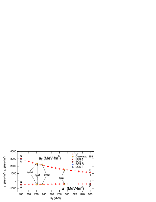
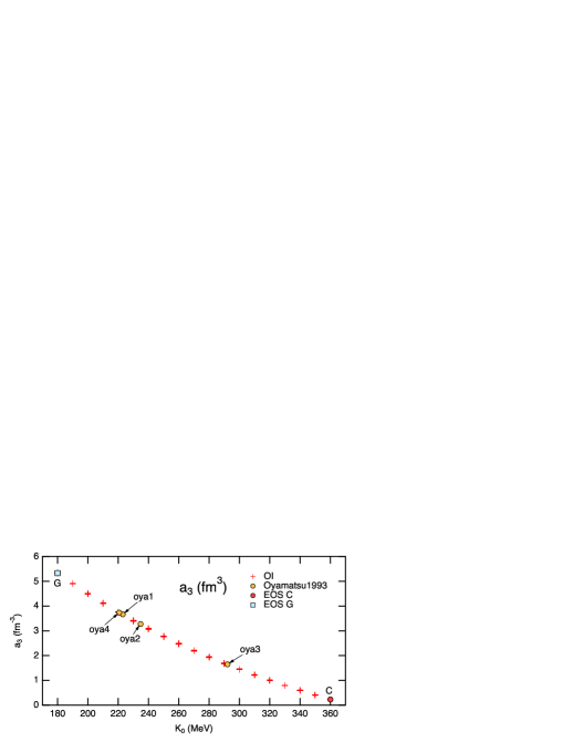
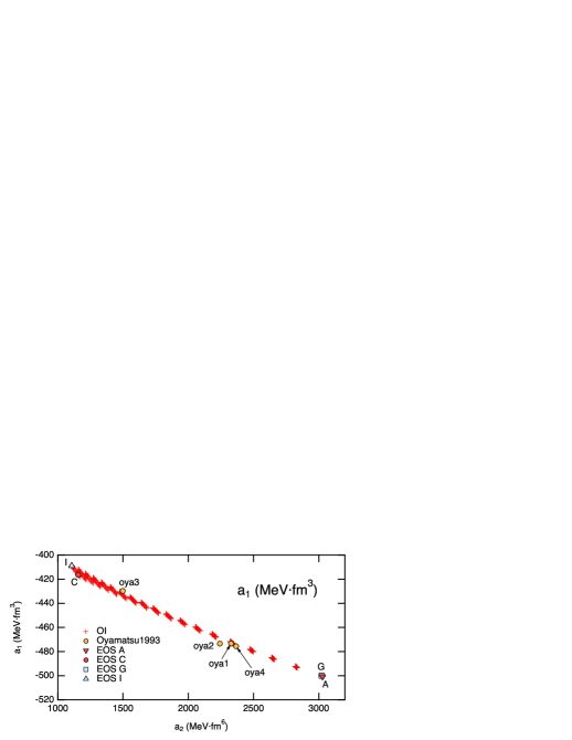
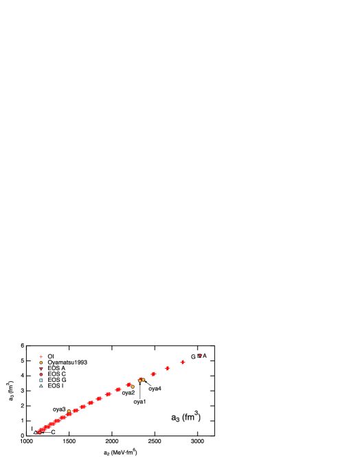
Figure 4: The potential parameters $a_{1}-a_{3}$ as functions of $K_{0}$ (upper), and $a_{1},a_{3}$ as functions of $a_{2}$ (lower). Also plotted are the four models (oya1-4) in the early study oya1993 , and EOSs A, C, G, and I in Table 2.

Figure 5: The potential parameters $b_{1}$ and $b_{2}$ as functions $L$ (upper), and $b_{1}$ as function of $b_{2}$ (lower). Also plotted are the four models (oya1-4) in the early study oya1993 and EOSs C and G in Table 2.

3.2 Values of saturation parameters and their correlations

Figure 6 shows the $K_{0}$ correlations of the saturation parameters $n_{0},w_{0}$, and $Q_{0}$ of symmetric matter. Naturally, these parameters correlate with $K_{0}$ because the potential parameters $a_{1}-a_{3}$ of the symmetric matter EOS $w_{s}(n)$ correlate with $K_{0}$. The saturation density $n_{0}$ shows a relatively clear correlation with $K_{0}$ in Fig. 6, except for appreciable sensitivities to $L$ at $K_{0}\gtrsim$300 MeV. On the other hand, the saturation energy $w_{0}$ is well constrained within about $\pm 0.1$ MeV and has subtle but relatively clear sensitivity to $K_{0}$ and $L$. This sensitivity is not negligible in the sense that 0.05 MeV/nucleon difference in ²⁰⁸Pb amounts to a 10 MeV difference of its mass excess.

For $Q_{0}$, we also see its clear correlation with $K_{0}$ in Fig. 6. Note that neither $K_{0}$ nor $Q_{0}$ includes the two-body energy coefficient $a_{1}$, so we expect a simple relation between $K_{0}$ and $Q_{0}$ in the OI model (see Eqs. (46) and (47)). Eventually, except for the subtle $L$ dependences for $n_{0}$ ($K_{0}\gtrsim 300$ MeV) and $w_{0}$, we confirm again that the symmetric matter EOS mainly depends on $K_{0}$.

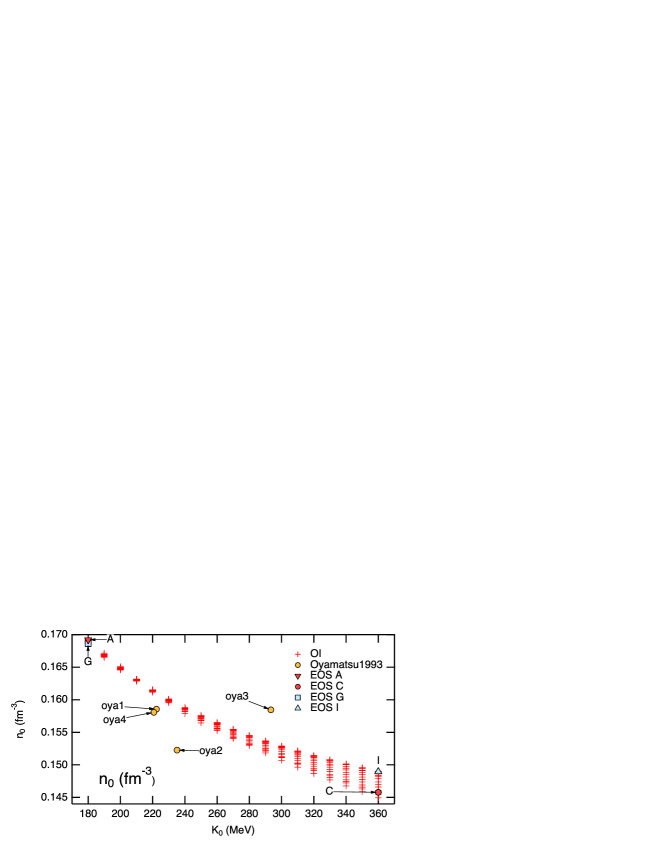
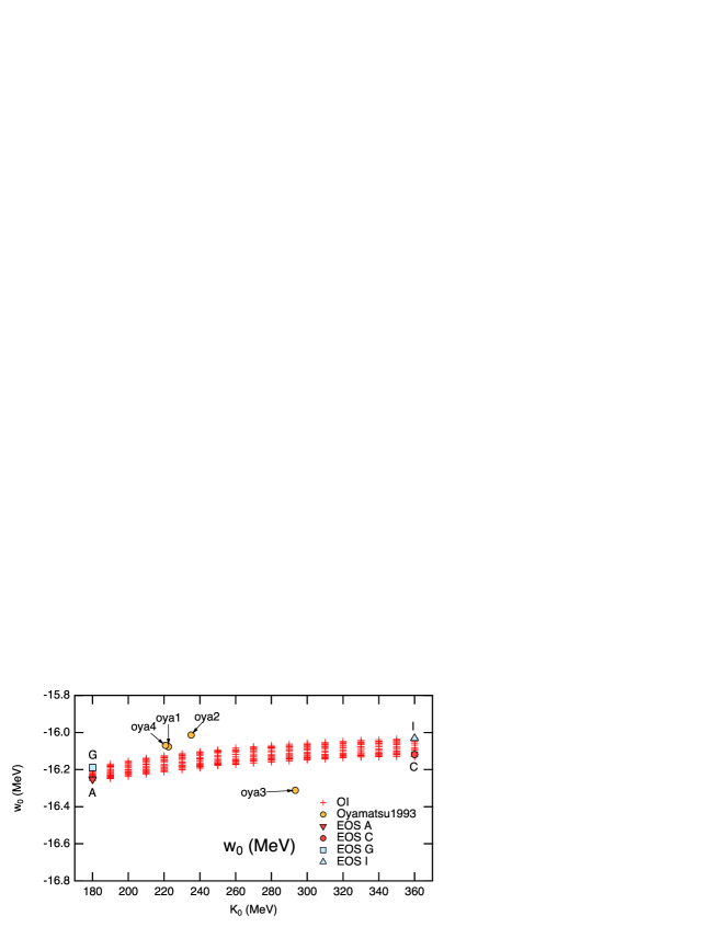
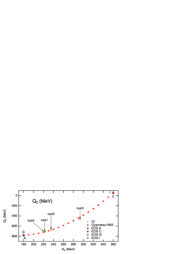
Figure 6: The $K_{0}$ correlations of the saturation parameters $n_{0},w_{0}$ and $Q_{0}$. Also plotted are the four models (oya1-4) in the early study oya1993 , and EOSs A, C, G, and I in Table 2.

Figure 7 shows the $L$ correlations of saturation parameters $w_{n0},L_{n0},K_{n0}$, and $Q_{n0}$ of neutron matter. Naturally, these parameters correlate with $L$ because the potential parameters $b_{1}-b_{3}$ of the neutron matter EOS $w_{n}(n)$ correlate with $L$. We see their strong correlations with $L$ in Fig. 7 and obtain the following fitting formulae:

$$w_{n0}=12.367\pm 0.0264+(0.075639\pm 0.000404)L\ \textrm{(MeV)},$$ (25)

$$L_{n0}=1.3611\pm 0.00316+(0.99956\pm 4.85\times 10^{-05})L\ \textrm{(MeV)},$$ (26)

$$K_{n0}=-74.636\pm 0.281+(3.7193\pm 0.00431)L\ \textrm{(MeV)},$$ (27)

$$Q_{n0}=(278.84\pm 0.739)+(-6.4345\pm 0.0113)L\ \textrm{(MeV)}.$$ (28)

The difference between $L_{n0}$ and $L$ is only 1 MeV, which is the kinetic energy of higher orders than $\alpha^{2}$. Finally, we remark that we have a simple relation between $K_{n0}$ and $Q_{n0}$ because the three-body coefficient $b_{2}$ is only one free parameter in Eqs. (52) and (53) (the $b_{3}$ value is fixed).

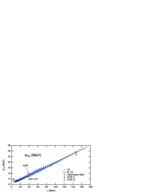
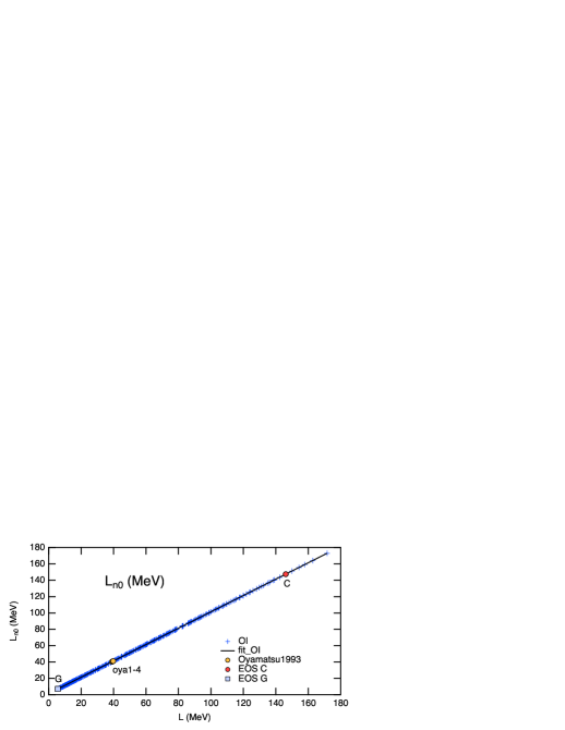
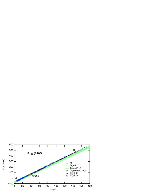
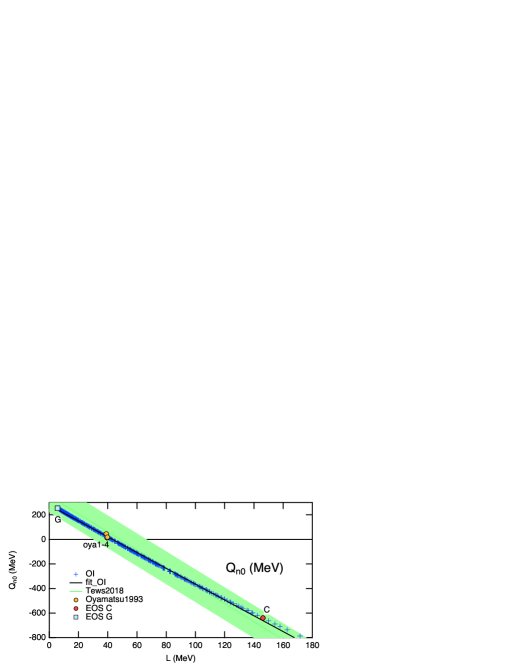
Figure 7: The $L$ correlations of the saturation parameters $w_{n0},L_{n0},K_{n0}$, and $Q_{n0}$. Their fitting lines (fit_OI) are also shown. The shaded areas (Tews2018) for $K_{n0}$ and $Q_{n0}$ are calculated with the fitting formulae by Tews et al. TewsLattimerOhnishiKolomeitsev2018 , which enclose 68.3% of their accepted interactions. We also plot the four models (oya1-4) in the early study oya1993 and EOSs C and G in Table 2.

Figure 8 shows the $L$ correlations of the saturation parameters $S_{0},K_{sym}$, and $Q_{sym}$, of the density-dependent symmetry energy $S(n)$. Except for $S_{0}$, the saturation parameters of $S(n)$ also have clear $K_{0}$ dependence from $w_{s}(n)$ because $S(n)\approx w_{n}(n)-w_{s}(n)$. The symmetry energy $S_{0}$ has a simple correlation with $L$ and is approximately given by

$$S_{0}=27.809\pm 0.0291+(0.0761\pm 0.000446)L\ \textrm{(MeV)}.$$ (29)

The values of the coefficients in Eq. (29) are slightly different but essentially the same as those in our previous study OI2003 . This simple correlation (29) stems from the fact that the saturation energy $w_{0}$ is essentially constant of $K_{0}$ and $L$ so that $S_{0}\approx w_{n0}-w_{0}$ reflects the $L$ dependence in $w_{n0}$ except for subtle $K_{0}$ dependence.

The saturation parameters $K_{sym}$ in Eq. (58) and $Q_{sym}$ in Eq. (59) have relatively complicated dependence on $K_{0}$ and $L$ because they include both $K_{0}$-dependent potential parameters $a_{2}-a_{3}$ and $L$-dependent $b_{2}$ (the value of $b_{3}$ is fixed). It is also noted that $K_{sym}$ and $Q_{sym}$ do not include two-body parameters.

The shaded areas for $K_{n0},Q_{n0}$, and $S_{0}$ in Figs. 7 and 8 are calculated with fitting formulae by Tews et al. TewsLattimerOhnishiKolomeitsev2018 , which enclose 68.3% of their accepted 188 Skyrme and 73 RMF interactions. These figures show that the saturation parameter values of neutron matter EOS in the OI model are consistent with the general trends of the phenomenological interactions.

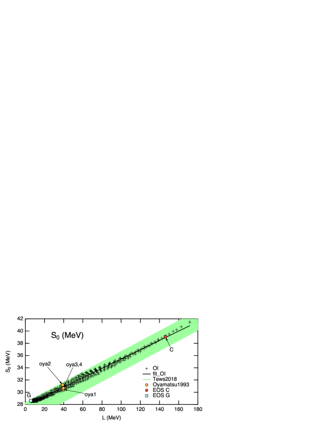
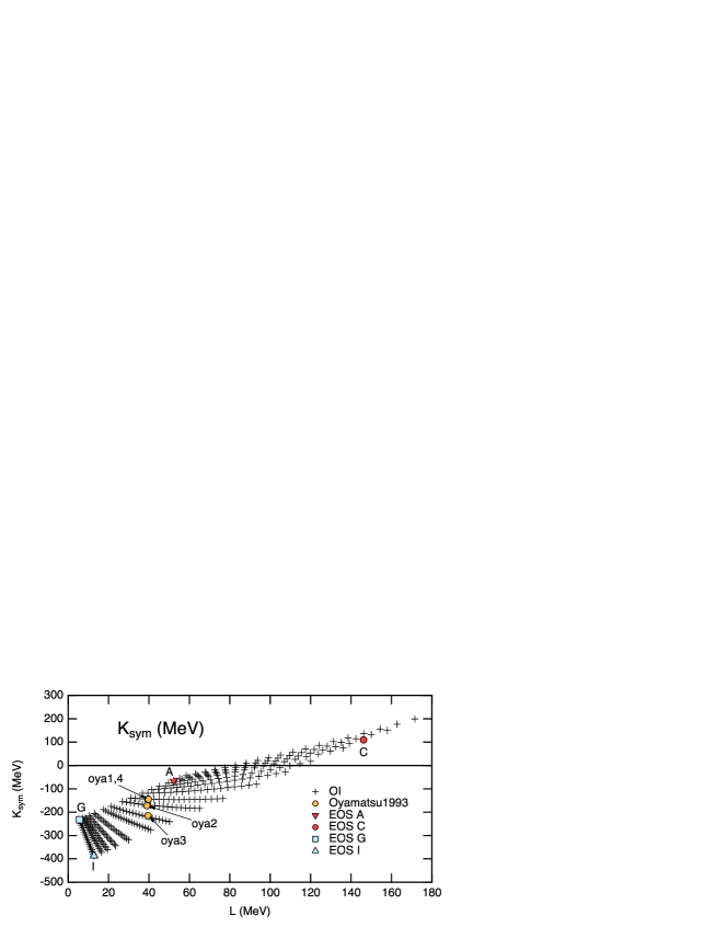
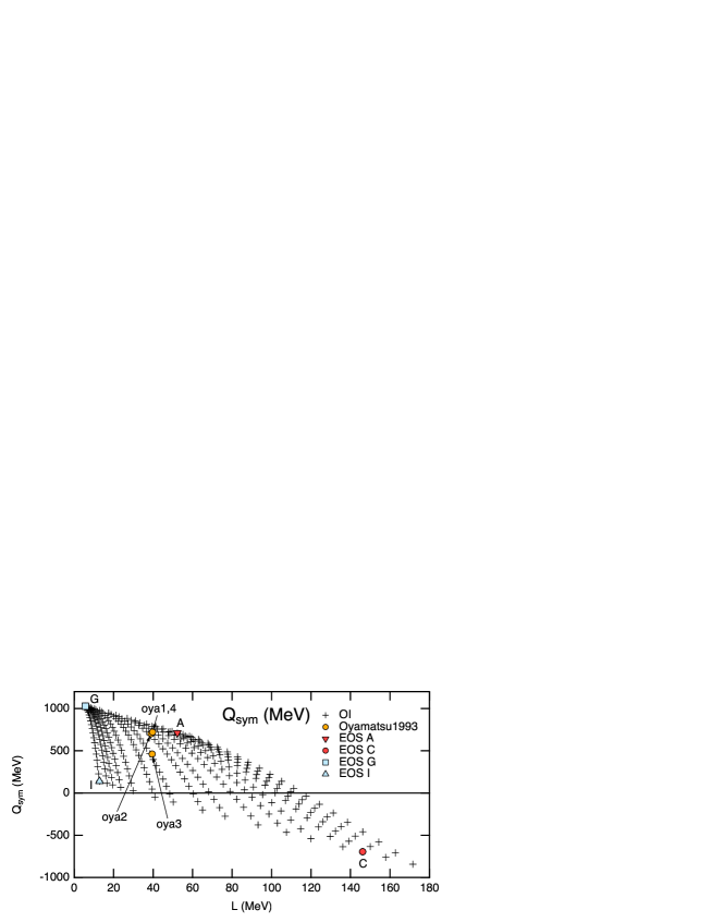
Figure 8: The $L$ correlations of the saturation parameters $S_{0},K_{sym}$, and $Q_{sym}$. Also plotted are the four models (oya1-4) in the early study oya1993 and EOSs A, C, G, and I in Table 2. The shaded area for $S_{0}$ is calculated with the fitting formula by Tews et al. TewsLattimerOhnishiKolomeitsev2018 , which encloses 68.3% of their accepted interactions.

3.3 Fixed points of $S(n)$ and $w_{n}(n)$

The $S_{0}-L$ correlation in Eq. (29) implies that the symmetry energy should have a reasonable value at the nuclear surface. Actually, in the lowest approximation,

$$S(n)\approx S_{0}+uL=27.809+(0.0761+u)L.$$ (30)

The symmetry energy at $u=-0.0761$ ($n/n_{0}=0.7717$) is constant (27.809 MeV) independently of $L$. Thus with the $S_{0}-L$ correlation (29), we have practically only one degree of freedom for $S(n)$ at $n\simeq n_{0}$ and choose the slope $L$ as the independent EOS parameter to study the nuclear structure.

Similarly, from the $w_{n0}-L$ correlation (25) and the $L_{n0}-L$ correlation (26) for neutron matter, we have, in the lowest approximation,

$$w_{n}(n)\approx w_{n0}+uL_{n0}\approx 12.367+1.3611u+(0.075639+0.99956u)L.$$ (31)

Then, the neutron-matter energy at $u=-0.0757$ ($n/n_{0}=0.7730$) is constant (12.264 MeV) independently of $L$. This property is an empirical constraint of neutron matter EOS, which Brown discussed using phenomenological interactions ABrown2000 . We mention that this constraint is obtained only from the empirical mass and radius data of stable nuclei in the present study.

3.4 Inhomogeneity energy and saturation parameters

The $w_{0}-F_{0}$ relation in Fig. 9 (upper) represents the correlation between uniform-matter and inhomogeneity energies of isoscalar interaction. Interestingly, the inhomogeneity energy parameter $F_{0}$ has complicated sensitivities to $K_{0}$ and $L$ (Fig. 9 (lower)). In contrast, the saturation energy $w_{0}$ is almost constant, showing only subtle sensitivities to $K_{0}$ and $L$ in Fig. 6. Despite these different sensitivities to $K_{0}$ and $L$, the $w_{0}-F_{0}$ correlation is natural because the potential contribution of the inhomogeneity energy is well represented by gradient expansion, whose coefficients are the spacial moments of the long-range part of inter-nucleon potentials Brueckner:1968zzb . In the OI model, we assume that the kinetic contribution is effectively included in the parameter $F_{0}$.

In principle, the choice of different inhomogeneity energy terms can make differences in the saturation density $n_{0}$ and energy $w_{0}$ because the inhomogeneity energy affects the local pressure equilibrium in a nucleus. Here we discuss the sensitivity of the inhomogeneity energy using the oya1-4 models of the early study oya1993 in Table 2 (see also Appendix C), keeping in mind that the optimization was probably poorer than the present one.

• The oya4 model has the same inhomogeneity energy as the OI model.

• The oya1-3 models have the kinetic contribution of the inhomogeneity energy in addition to the potential contribution.

• The oya2 model also includes an extremely large isovector gradient term.

• The $K_{0}$ and $L$ ($-y$) values of the oya1-4 models were also optimized with the additional constraint $b_{1}/b_{2}=-0.3232$ (fm^-3).

The values of the potential and saturation parameters of all oya1-4 models in Figs. 4-8 agree well with those of the OI model except for the slight differences in the $n_{0}$ and $w_{0}$ values in Figs. 6 and 9. Notably, the excellent agreement of the oya1 and oya4 results encourages our assumption that the kinetic contribution of the inhomogeneity can be effectively included in the coefficient $F_{0}$. Furthermore, the neutron matter EOS parameters of all oya1-4 in Figs. 5 and 7 agree very well ($L\approx 40$ MeV), so the neutron matter EOS seems insensitive to the inhomogeneity energy even with the large isovector inhomogeneity energy in the oya2 model. Interestingly, the oya2 values of the symmetric matter EOS parameters in Figs. 4 and 6 differ from the oya1 and oya4 values. Hence, the isovector inhomogeneity energy cancels the isoscalar inhomogeneity energy and affects the symmetric matter EOS (see Table 2 and Appendix C).

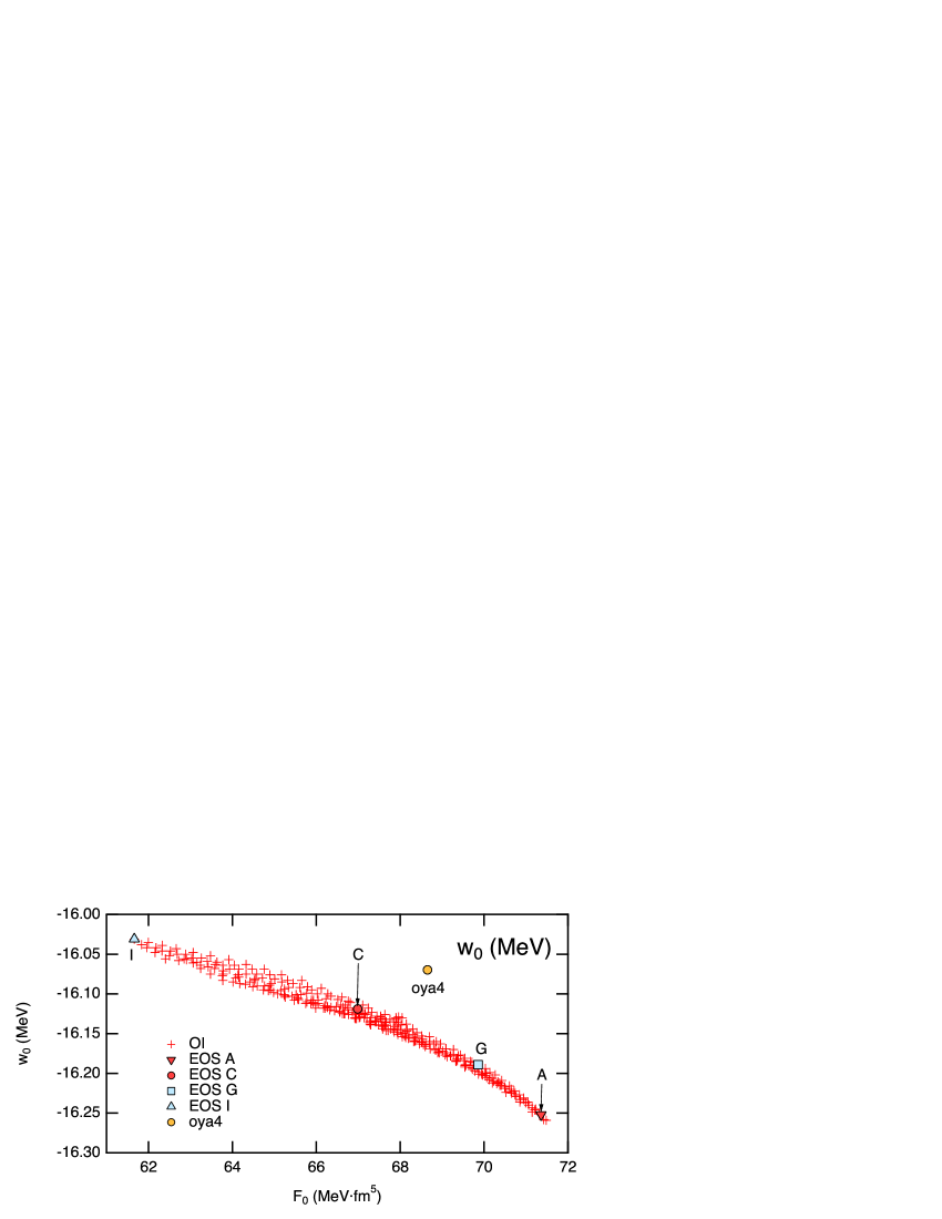
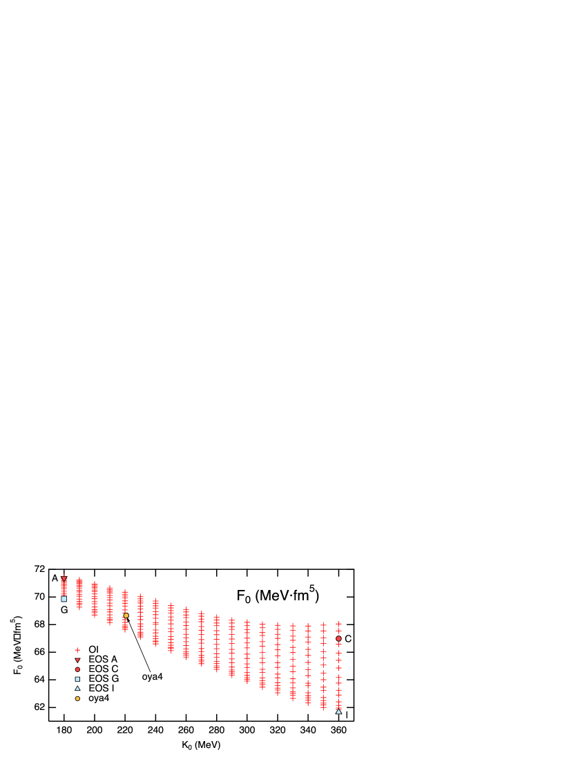
Figure 9: The correlations between $w_{0}$ and $F_{0}$ (upper) and between $F_{0}$ and $K_{0}$ (lower). Also plotted are the oya4 in the early study oya1993 and EOSs A, C, G, and I in Table 2.

3.5 Nuclear masses and the empirical EOSs

Figure 10 shows the nuclides with $A\geq 40$, whose experimental mass values are compared with the calculated values using the OI model’s update 304 interactions (EOSs); 2301 nuclides in Atomic Mass Evaluation 2020 (AME2020)Wang:2021xhn , 1514 nuclides in AME1983Wapstra:1985hmr together with 211 most stable isobars with $40\leq A\leq 250$. We exclude the lighter nuclei because the OI model overestimates their masses, as shown in Fig. 14 (upper). Figure 11 shows the mean deviations (upper) and root-mean-square deviations (lower) from the experimental mass values in AME2020 and AME1983. The mean and rms deviations for the most stable isobars (MSIs) are also plotted in Figure 11. The mean deviation for MSIs is almost constant of $L$ at about 1.2–1.6 MeV but shows appreciable scattering, presumably reflecting the strong shell effects in the MSIs. The rms deviation for the MSIs is also almost constant at about 3.1 – 3.2 MeV and much larger than 1.1 – 2.3 MeV for the smoothed data in Fig. 3. The mean deviation for the AME2020 nuclides is less than 1 MeV and shows a clear dependence on $L$. Meanwhile, the rms deviation for the AME2020 nuclides is about 3 MeV at $L\lesssim 90$ MeV but increases with $L$ clearly at $L>90$ MeV. These values are small as a semiclassical theory, which neglects shell energies of the order of MeV.

The mass deviations are significant for the MSIs, whose masses are lowered by the relatively large shell energies, with minor sensitivity to $L$. Meanwhile, for unstable nuclei, the sensitivity to $L$ emerges with neutron-richness Oyamatsu:2010bf , and the shell effects diminish. This is the origin of the $L$-sensitivity of the mean deviation. The AME1983 nuclides lay close to the MSIs. The mean and rms deviations and their $L$ dependences for the AME1983 nuclides are between those for the MSIs and AME2020 nuclides. It is noteworthy that if we compare the rms deviations for the AME1983 and AME2020 nuclides, the progress of the mass evaluation in the last about 40 years reveals that the preferred value of $L$ would roughly lay between 20 and 90 MeV. However, the lower bound is not constrained well by the nuclear mass data of unstable nuclei. This range is consistent with the evaluations by Lattimer and Lim Lattimer:2012xj and with recent experimental estimates of the $L$ value, which still have significant uncertainties. From the Sn+Sn reaction, Estee et al. estimate $42<L<117$ MeV SRIT:2021gcy . From the parity violating asymmetry in ²⁰⁸Pb, Reed et al. estimate $L=106\pm 37$ MeV Reed:2021nqk , while Reinhard et al. analyze the same experimental data and evaluate $L=54\pm 8$ MeV Reinhard:2021utv .

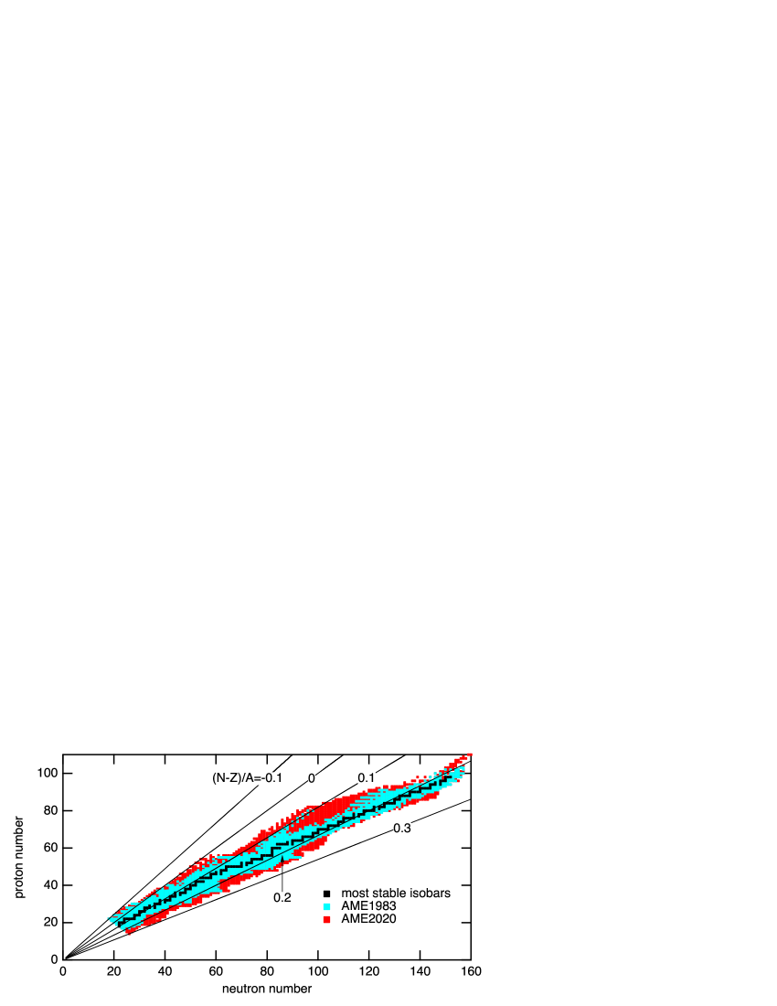
Figure 10: The nuclides with $A\geq 40$, whose masses are calculated and compared with the experimental values in AME1983Wapstra:1985hmr and AME2020Wang:2021xhn . We only calculate the masses of the most stable isobars with $40\leq A\leq 250$.

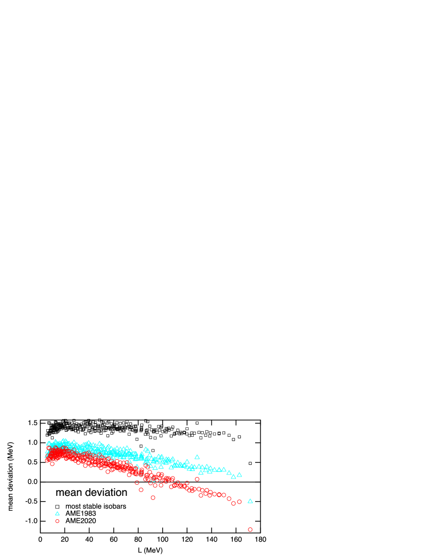
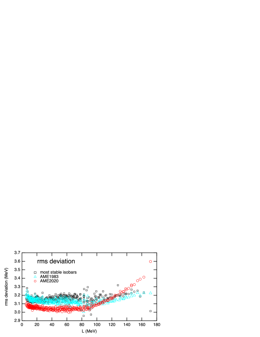
Figure 11: The mean deviations (upper) and the rms deviations (lower) of the calculated masses from the experimental ones as functions of $L$. The nuclear mass calculations were performed for the most stable isobars, the AME1983 nuclidesWapstra:1985hmr and the AME2020 nuclidesWang:2021xhn in Fig. 10.

4 Liquid-drop energies in the OI model

4.1 Incompressible liquid-drop mass formula

The proton, neutron, and mass numbers are continuous variables in this section. The incompressible liquid drop (ILD) mass formula gives the mass excess as

$$M_{ex\_ILD}=a_{v}A+a_{I}\frac{(N-Z)^{2}}{A}+a_{surf}A^{2/3}+a_{C}\frac{Z^{2}}{A^{1/3}}+\Delta m.$$ (32)

The volume energy $a_{v}$ is close to the saturation energy $w_{0}$ of symmetric nuclear matter. The surface energy coefficient $a_{surf}$ is related to the gradient energy coefficient $F_{0}$ in Eq. (17). The symmetry energy coefficient $a_{I}$ is smaller than $S_{0}$ because it includes the energy of low-density matter at the surface. The Coulomb energy coefficient $a_{C}$ is related to nuclear size, hence to the saturation density $n_{0}$. The values of these four liquid drop coefficients are constrained well from nuclear masses. In this paper, we adopt the coefficient values of Yamada’s reference ILD mass formula MYamada1964 in Table 3, which was determined from the overall fits of the $\beta$-stability line and the mass excesses of $\beta$-stable nuclei. Appendix B gives explicit formulae for neutron excess, mass, and radius of a nuclide on the smoothed $\beta$ stability line, and their calculated values with the coefficient values in Table 3.

Table 3: The coefficient values in MeV of Yamada’s reference ILD mass formulaMYamada1964 .

$a_{v}$	$a_{C}$	$a_{I}$	$a_{s}$
-15.88485	0.71994	23.64332	18.32695

Table 4: The energy parameters of the OI and ILD models, together with saturation parameters.

	symmetric matter	neutron matter	symmetry energy	finite range
interaction	isoscalar	isoscalar+isovector	isovector	isoscalar
OI	$a_{1},\ a_{2},\ a_{3}$	$b_{1},\ b_{2}(,\ b_{3})$	$a_{1}-a_{3},\ b_{1},\ b_{2}(,\ b_{3})$	$F_{0}$
ILD	$a_{v},\ a_{C}$	$a_{v}+a_{I}$	$a_{I}$	$a_{s}$
saturation	$n_{0},\ w_{0},\ K_{0}$	$w_{n0},\ L_{n0}$	$S_{0},\ L$

Table 4 summarizes the energy parameters in the OI and ILD models together with saturation parameters. For fixed $K_{0}$ and $L$, the OI model has the same degrees of freedom ($n_{0},w_{0},S_{0}$, and $F_{0}$) as the ILD model. Consequently, we can construct a family of the EOSs as a function of $(K_{0},L)$ by fitting nuclear masses. Furthermore, the five potential parameters, $a_{1}-a_{3},b_{1}$, and $b_{2}$, can be calculated analytically from the five saturation parameters,$n_{0},w_{0},K_{0},S_{0},L$, and $b_{3}$, as shown in Appendix A.4. Therefore, the interaction parameters are also functions of $(K_{0},L)$.

4.2 Mapping to liquid drop energies

In this section, we show how the surface, symmetry, and volume energies of the ILD model are represented in the OI model. If necessary, the subscripts ”_ILD” and ”_OI” distinguish the models explicitly.

We use the size-equilibrium condition for the most stable nuclide to define the surface energy, $W_{surf\_OI}$ of the most stable nuclide. In the ILD model, from the condition that $M_{ex}/A$ is minimum with respect to $A$ keeping $(N-Z)/A$ constant, we obtain the relation,

$$W_{surf}=2W_{C}$$ (33)

between the surface energy $W_{surf}$ and the Coulomb energy $W_{C}$. In the OI model, from the size equilibrium condition for $M_{ex}/A$ (see Appendix D), we obtain a similar relation between the gradient and Coulomb energies as

$$W_{g}=W_{C\_OI}.$$ (34)

Assuming the relation (33) also in the OI model, we obtain the surface energy of the OI model using Eqs. (34) and (17).

$$W_{surf\_OI}=2W_{g}=2\int d^{3}rF_{0}|\nabla n(r)|^{2}.$$ (35)

The liquid-drop symmetry energy of the OI model, $W_{i\_OI}$, is the isovector part of the uniform-matter energy $W_{EOS}$.

$$W_{i\_OI}=\int d^{3}r\left[\epsilon_{0}\left(n_{n}(r),n_{p}(r)\right)-\epsilon_{0}\left(n(r)/2,n(r)/2\right)\right].$$ (36)

Finally, the volume energy of the OI model, $W_{v\_OI}$, is the remaining energy given by

$$W_{v\_OI}=W_{EOS}+W_{g}-W_{surf\_OI}-W_{i\_OI}=\int d^{3}r\left[\epsilon_{0}\left(n(r)/2,n(r)/2\right)-F_{0}|\nabla n(r)|^{2}\right],$$ (37)

which is desirable isoscalar energy. Equations (35) and (37) suggest that half of the surface energy comes from the EOS energy.

Figure 12 shows the OI and ILD energies per nucleon of the most stable nuclide; $w_{EOS}=W_{EOS}/A$, $w_{surf}=W_{surf}/A$, $w_{C}=W_{C}/A$, $w_{i}=W_{i}/A$, $w_{v}=W_{v}/A$, and the mass excess per nucleon $m_{ex}=M_{ex}/A$. These OI energies per nucleon are nearly constant of $L$ (and $K_{0}$) and almost equal to the ILD energies. We see that the OI model is a natural extension of the ILD model from the excellent agreement of the four liquid-drop energies, the surface, Coulomb, symmetry, and volume energies.

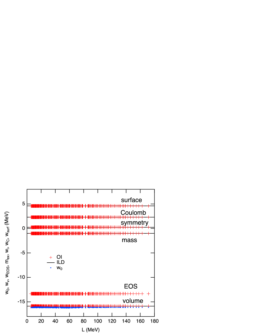
Figure 12: The liquid-drop energies of the most stable nuclide as functions of $L$. The red crosses (OI) show OI model calculations, while the horizontal lines (ILD) are the results obtained with the coefficient values of the reference ILD model in Table 3. The blue dots ($w_{0}$) show the saturation energy $w_{0}$ of the OI model interactions.

As shown in Fig. 12, the volume energy per nucleon $w_{v}$ is close to the saturation energy $w_{0}$ and surprisingly constant, presumably reflecting correlations among symmetric matter EOS (isoscalar) parameters, including $w_{0}-F_{0}$. Hence, the existence of the surface does not affect the liquid-drop core appreciably, thanks to the appropriate definitions of the surface and volume energies in Eqs. (35) and (37).

Figure 13 shows that the OI model energies, even for two extreme EOSs C and G, also agree with the corresponding ILD energies as functions of mass number A. The agreement is excellent in the range of $A\gtrsim 40$. Consequently, Fig. 14 shows that the OI model values of the mass excess per nucleon $m_{ex}$ (upper) and the neutron excess ratio $(N-Z)/A$ (lower) also agree well with the experimental values.

Unfortunately, the OI and ILD models overestimate the mass excesses at $A\lesssim 40$, as shown in Fig. 14 (upper). The increase of $w_{v\_OI}$ with the decrease of $A$ implies that a better description of the surface energy is necessary. The OI model’s interaction and density distribution must be too crude to describe a light nucleus with $A\lesssim 25$, which has a small core compared to the surface and reduces its energy primarily by quantum mechanical effects.

Interestingly, the $(N-Z)/A$ values at $A\gtrsim 200$ of the two extreme OI models are almost equal but slightly different from that of the ILD. The neutron excess is mainly determined from the symmetry and Coulomb energies, and in the ILD model, it is given by

$$\frac{I}{A}=\frac{a_{c}A^{2/3}-(m_{n}-m_{p}-m_{e})}{a_{c}A^{2/3}+4a_{I}}.$$ (38)

In Fig. 14, the Coulomb and symmetry energies of the ILD and the OI models (EOSs C and G) agree well. In contrast, the surface and, consequently, volume energies (see Eq. (37)) of the EOSs C and G are slightly different from those of the ILD model. Hence, the slight neutron excess difference at $A\gtrsim 200$ between the ILD and OI models might be induced by the surface distribution difference (including the neutron skin) .

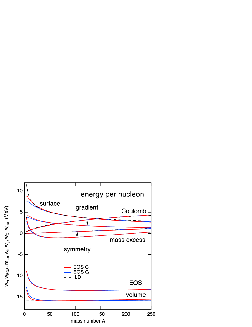
Figure 13: The energies of the most stable isobars as functions of $A$. The red and blue lines show OI model calculations with two extreme EOSs C and G, while the black dashed lines are the results obtained with the reference ILD model. These three lines are almost indistinguishable except for the surface, gradient, and volume energies at small or large A values.

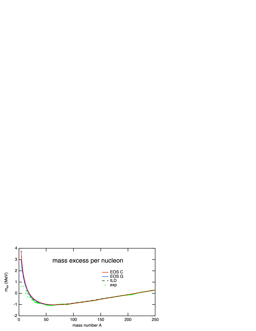
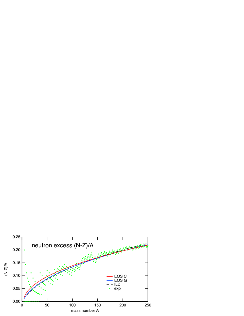
Figure 14: The mass excess per nucleon $m_{ex}$ and the neutron excess ratio $(N-Z)/A$ of the most stable isobars as functions of mass number $A$. The red and blue lines show the OI model calculations with two extreme EOSs C and G, while the black dashed lines are the reference ILD model calculations. The green dots show the experimental values.

4.3 Most stable nuclide in the OI and ILD models

Figure 15 (upper) shows that the most stable nuclides in the OI and ILD models are heavier than the empirical ⁵⁶Fe ($Z=26$ and $A=56$). These deviations are not surprising because the shell energy significantly shifts the minimum point. In contrast, the smoothed energy per nucleon varies slowly around the minimum, as shown in Fig. 14. Even for the KTUY mass formula Koura2005 , the gross part of KTUY mass per nucleon is minimum at $Z=28$ and $A=62$. Figure 15 (lower) shows that the proton, neutron, and matter radii are almost constant except for subtle $L$ dependence related to neutron skin formation. We note that the proton radius is almost constant of $K_{0}$ and $L$ because we fit the empirical charge radius data.

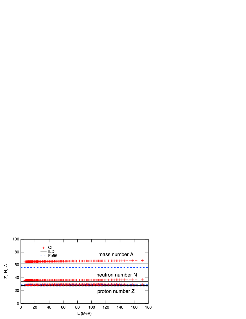
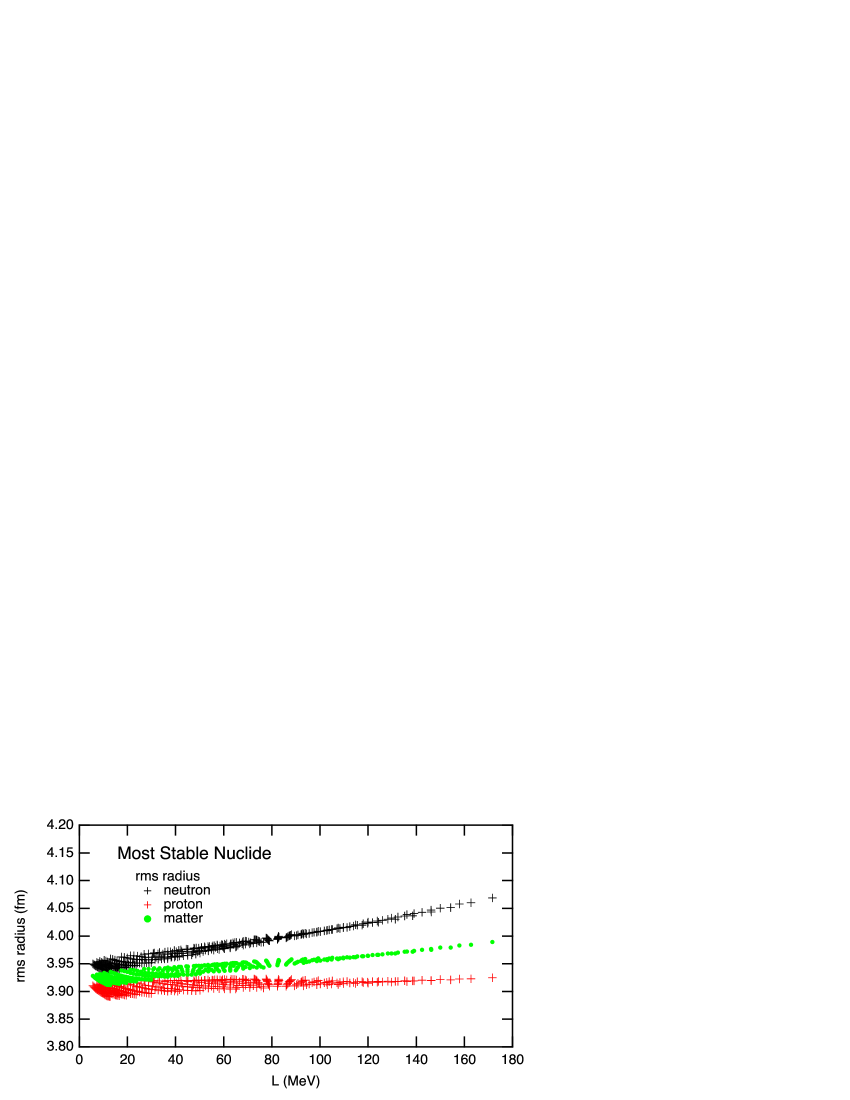
Figure 15: The mass, neutron, and proton numbers (upper) and the rms radii (lower) of the most stable nuclide as functions of $L$. The crosses show the OI model calculations, while the black horizontal lines are the results of the reference ILD model.

Lastly, we mention that the point nucleon distribution (Eq. (19)) of the most stable nucleus has a reasonable surface thickness, although we imposed no constraint on the thickness in optimizing the OI model parameters. Figure 16 shows the 90%-10% surface thicknesses of the neutron and proton distributions denoted by thick(neutron) and thick(proton), together with the average of the two thicknesses as a rough estimate of the thickness of the matter distribution.

$$\textrm{thick(average)}=\frac{N}{A}\textrm{thick(neutron)}+\frac{Z}{A}\textrm{thick(proton)}.$$ (39)

These three thicknesses correlate clearly with $K_{0}$ (upper box) and appreciably with $F_{0}$ (lower box). These correlations reflect that $K_{0}$ and $F_{0}$ are the lowest-order parameters contributing to the surface energy. While the surface energy agrees well between the OI and ILD models, the proton and average thickness values are slightly smaller than the empirical value of 2.4 fm in most cases OI2003 .

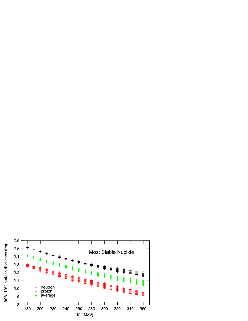
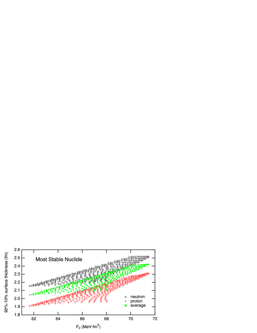
Figure 16: The 90%-10% surface thicknesses of the point-neutron and point-proton distributions as functions of $K_{0}$ (upper) and $F_{0}$ (lower). Also shown is the average of these two thicknesses as a rough estimate of the matter distribution (Eq. (39)).

5 Conclusions

This paper studies how nuclear masses are affected by the equation of state of nuclear matter. We adopt a macroscopic nuclear model, named the OI model, with reasonable many-body energy and isoscalar gradient energy. We use 304 update interactions, covering wide ranges of the incompressibility $K_{0}$ and the density-slope $L$. For fixed $K_{0}$ and $L$, the OI model has the same number of independent interaction parameters as the ILD model. Moreover, all the OI interactions almost equally fit empirical mass, neutron excess, and radius data of stable nuclei, nearly insensitively of $K_{0}$ and $L$.

This insensitivity is consistent with the ILD picture and leads to the correlations among interaction and saturation parameters. We found that the interaction and saturation parameters of symmetric nuclear matter correlate mainly with $K_{0}$, and those of neutron matter mainly with $L$.

We assume that the surface energy of the OI model is twice as large as the gradient energy using the size equilibrium conditions of the ILD and OI models. Then, the two models’ volume, surface, symmetry, and Coulomb energies agree very well for the most stable isobars with $A\geq 40$.

The correlation between the saturation energy $w_{0}$ and the gradient energy coefficient $F_{0}$ probably works to define the volume and surface energies properly. Meanwhile, the well-known strong correlation between $S_{0}$ and $L$ helps explain the symmetry energy agreement between the ILD and OI models. Furthermore, the latter correlation causes the fixed points of the density-dependent symmetry energy and neutron matter EOS.

While calculated masses in the OI model are essentially insensitive to $K_{0}$ and $L$ for nuclei close to the $\beta$-stability line, they are relatively sensitive to $L$ for unstable nuclei. Interestingly, the OI model with $L\lesssim 100$ MeV predicts the latest mass data better than those of stable nuclei, and we suggest $20\lesssim L\lesssim 90$ MeV, although the lower boundary is not constrained well.

Presumably, the conclusions of this paper are not affected significantly by our choice of the empirical data of stable nuclei, the many-body energy, or the inhomogeneity energy because the correlations among the saturation parameters of the OI model are consistent with relativistic and non-relativistic phenomenological interactions of contemporary use.

We have extensively performed the neutron star matter calculation with the OI model and have reported preliminary results in Refs. Oyamatsu:2017qzv and Oyamatsu:2020dlb . We are preparing to publish the final results with discussions along the line of this paper.

Appendix A Explicit formula of saturation parameters and potential parameters

Our previous paper OI2003 simplified the kinetic energy expression by using the neutron mass as the proton mass because this replacement gives a relatively small effect. Meanwhile, the numerical calculations in the paper were performed using the real proton mass. In this paper, we write the neutron and proton rest masses explicitly.

The neutron-proton mass difference forces us to use some prescription for the definition of the density-dependent symmetry energy $S(n)$ because the kinetic energy density in $\epsilon_{0}(n_{n},n_{p})$ (Eq. (1)) is not charge-symmetric, and

$$\frac{\partial w(n,\alpha)}{\partial\alpha}\bigg{|}_{\alpha=0}\neq 0.$$ (40)

To keep the charge symmetry, we use the value of the nucleon rest mass of

$$m=\frac{m_{n}+m_{p}}{2},$$ (41)

when and only when we calculate $S(n)$ and its saturation parameters. This prescription increases the kinetic energy by $5\times 10^{-5}$%.

A.1 Symmetric matter EOS $w_{s}(n)$

The proton rest mass $m_{p}$ and the neutron rest mass $m_{n}$ are used.

$$w_{s}(n)=c_{s}n^{2/3}+a_{1}n+\frac{a_{2}n^{2}}{1+a_{3}n},$$ (42)

with

$$c_{s}=\frac{3}{10}\left(\frac{3\pi^{2}}{2}\right)^{2/3}\left(\frac{\hbar^{2}}{2m_{n}}+\frac{\hbar^{2}}{2m_{p}}\right).$$ (43)

$$w_{0}=c_{s}n_{0}^{2/3}+a_{1}n_{0}+\frac{a_{2}n_{0}^{2}}{1+a_{3}n_{0}}.$$ (44)

$$L_{0}=3n_{0}\frac{dw_{s}}{dn}\Big{|}_{n=n_{0}}=2c_{s}n_{0}^{2/3}+3a_{1}n_{0}+\frac{3a_{2}n_{0}^{2}(2+a_{3}n_{0})}{(1+a_{3}n_{0})^{2}}=0.$$ (45)

$$K_{0}=9n_{0}^{2}\frac{d^{2}w_{s}}{dn^{2}}\Big{|}_{n=n_{0}}=-2c_{s}n_{0}^{2/3}+\frac{18a_{2}n_{0}^{2}}{(1+a_{3}n_{0})^{3}}.$$ (46)

$$Q_{0}=27n_{0}^{3}\frac{d^{3}w_{s}}{dn^{3}}\Big{|}_{n=n_{0}}=8c_{s}n_{0}^{2/3}-\frac{162a_{2}a_{3}n_{0}^{3}}{(1+a_{3}n_{0})^{4}}.$$ (47)

A.2 Neutron matter EOS $w_{n}(n)$

The neutron rest mass $m_{n}$ is used.

$$w_{n}(n)=c_{n}n^{2/3}+b_{1}n+\frac{b_{2}n^{2}}{1+b_{3}n},\quad c_{n}=\frac{3}{5}(3\pi^{2})^{2/3}\frac{\hbar}{2m_{n}},$$ (48)

with

$$c_{n}=\frac{3}{5}(3\pi^{2})^{2/3}\frac{\hbar^{2}}{2m_{n}}.$$ (49)

$$w_{n0}=c_{n}n_{0}^{2/3}+b_{1}n_{0}+\frac{b_{2}n_{0}^{2}}{1+b_{3}n_{0}}.$$ (50)

$$L_{n0}=3n_{0}\frac{dw_{n}}{dn}\Big{|}_{n=n_{0}}=2c_{n}n_{0}^{2/3}+3b_{1}n_{0}+\frac{3b_{2}n_{0}^{2}(2+b_{3}n_{0})}{(1+b_{3}n_{0})^{2}}.$$ (51)

$$K_{n0}=9n_{0}^{2}\frac{d^{2}w_{n}}{dn^{2}}\Big{|}_{n=n_{0}}=-2c_{n}n_{0}^{2/3}+\frac{18b_{2}n_{0}^{2}}{(1+b_{3}n_{0})^{3}}.$$ (52)

$$Q_{n0}=27n_{0}^{3}\frac{d^{3}w_{n}}{dn^{3}}\Big{|}_{n=n_{0}}=8c_{n}n_{0}^{2/3}-\frac{162b_{2}b_{3}n_{0}^{3}}{(1+b_{3}n_{0})^{4}}.$$ (53)

A.3 Density-dependent symmetry energy $S(n)$

The nucleon mass $m=(m_{n}+m_{p})/2$ is used as described at the beginning of this Appendix.

$$S(n)=\frac{\partial w}{\partial\alpha^{2}}\Big{|}_{\alpha=0}=c_{m}n^{2/3}+(b_{1}-a_{1})n+\frac{b_{2}n^{2}}{1+b_{3}n}-\frac{a_{2}n^{2}}{1+a_{3}n},$$ (54)

with

$$c_{m}=\frac{1}{3}\left(\frac{3\pi^{2}}{2}\right)^{2/3}\frac{\hbar^{2}}{2m}.$$ (55)

$$S_{0}=c_{m}n_{0}^{2/3}+(b_{1}-a_{1})n_{0}+\frac{b_{2}n_{0}^{2}}{1+b_{3}n_{0}}-\frac{a_{2}n_{0}^{2}}{1+a_{3}n_{0}}.$$ (56)

$$L=3n_{0}\frac{dS}{dn}\Big{|}_{n=n_{0}}=2c_{m}n_{0}^{2/3}+3(b_{1}-a_{1})n_{0}+\frac{3b_{2}n_{0}^{2}(2+b_{3}n_{0})}{(1+b_{3}n_{0})^{2}}-\frac{3a_{2}n_{0}^{2}(2+a_{3}n_{0})}{(1+a_{3}n_{0})^{2}}.$$ (57)

$$K_{sym}=9n_{0}^{2}\frac{d^{2}S}{dn^{2}}\Big{|}_{n=n_{0}}=-2c_{m}n_{0}^{2/3}+\frac{18b_{2}n_{0}^{2}}{(1+b_{3}n_{0})^{3}}-\frac{18a_{2}n_{0}^{2}}{(1+a_{3}n_{0})^{3}}.$$ (58)

$$Q_{sym}=27n_{0}^{3}\frac{d^{3}S}{dn^{3}}\Big{|}_{n=n_{0}}=4c_{m}n_{0}^{2/3}-\frac{162b_{2}b_{3}n_{0}^{3}}{(1+b_{3}n_{0})^{4}}+\frac{162a_{2}a_{3}n_{0}^{3}}{(1+a_{3}n_{0})^{4}}.$$ (59)

A.4 Potential parameters $a_{1},a_{2},a_{3},b_{1}$ and $b_{2}$

We calculate the potential parameters $a_{1},a_{2},a_{3},b_{1}$, and $b_{2}$ from the saturation parameters $n_{0},w_{0},K_{0},S_{0}$, and $L$, and the potential parameter $b_{3}$ using the following formula.

$$a_{3}=\frac{1}{n_{0}}\frac{4c_{s}n_{0}^{2/3}-18w_{0}-K_{0}}{2c_{s}n_{0}^{2/3}+K_{0}}.$$ (60)

$$a_{2}=\frac{(1+a_{3}n_{0})^{3}}{18n_{0}^{2}}\left(2c_{s}n_{0}^{2/3}+K_{0}\right).$$ (61)

$$a_{1}=\frac{1}{n_{0}}\left(w_{0}-c_{s}n_{0}^{2/3}-\frac{a_{2}n_{0}^{2}}{1+a_{3}n_{0}}\right).$$ (62)

$$b_{2}=\frac{(1+b_{3}n_{0})^{2}}{3n_{0}^{2}}\left[\frac{5}{9}c_{m}n_{0}^{2/3}+\frac{3a_{2}n_{0}^{2}}{(1+a_{3}n_{0})^{2}}-3S_{0}+L\right].$$ (63)

$$b_{1}=\frac{1}{n_{0}}\left(-\frac{5}{9}c_{m}n_{0}^{2/3}+a_{1}n_{0}+\frac{a_{2}n_{0}^{2}}{1+a_{3}n_{0}}-\frac{b_{2}n_{0}^{2}}{1+b_{3}n_{0}}+S_{0}\right).$$ (64)

Appendix B Comparison between the calculated and empirical values of $I$, $M_{ex}$, and $R_{ch}$

Figure 17 compares the calculated and empirical values of $I$, $M_{ex}$, and $R_{ch}$. The deviations from the empirical values are small compared with the scatterings due to shell effects even for two extreme EOSs C and G.

To compare the empirical and calculated values in detail in Fig. 17, we use the following reference formulae: approximate smoothed values of the neutron excess $I_{ref}$ KodamaYamada1971 , the mass excess $M_{ref}$ MYamada1964 ; KodamaYamada1971 , and the charge radius $R_{ref}$ as functions of mass number $A$.

$$I_{ref}=\frac{0.35997A^{2/3}-0.39131}{0.35997A^{2/3}+47.28664}\ A$$ (65)

$$\begin{split}M_{ref}=(7.68004-15.88485)A+0.39131I_{ref}+18.32695A^{2/3}\\ +23.64332\frac{I_{ref}^{2}}{A}+0.71994\frac{(A-I_{ref})^{2}}{4A^{1/3}}\end{split}$$ (66)

$$\begin{split}R_{ref}=0.665608+0.830616A^{1/3}-3.3634\times 10^{-3}A\\ +3.1635\times 10^{-5}A^{2}-8.0277\times 10^{-8}A^{3}\end{split}$$ (67)

Equation (67) was also used to calculate the empirical $R_{ch}^{emp}$ values in Table 1.

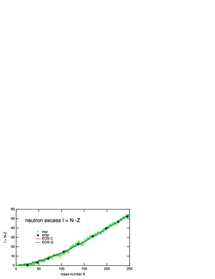
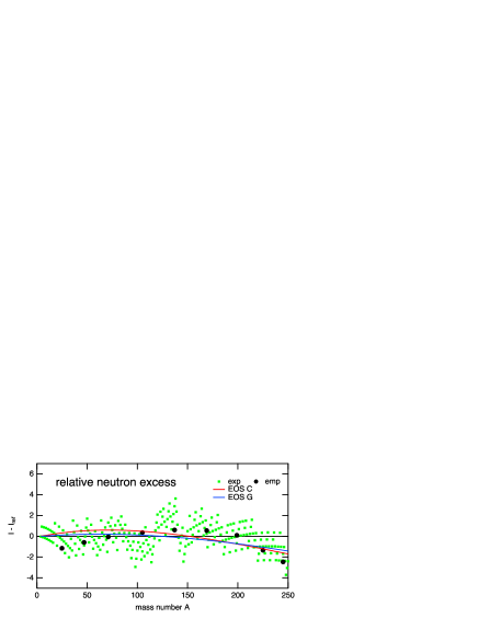
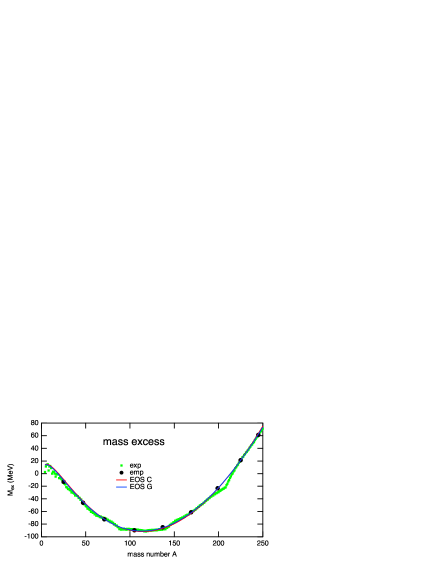
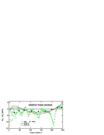
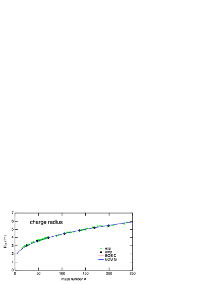
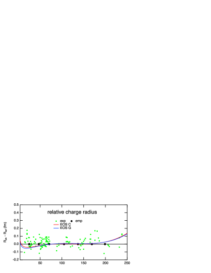
Figure 17: Comparison of the empirical (filled black circles) and calculated (lines) values of $I$, $M_{ex}$, and $R_{ch}$. The calculations are performed with two extreme EOSs C (red lines) and G (blue lines) in Table 2. For $I$ and $M_{ex}$, the experimental values of the most stable isobars Wang:2021xhn are also shown by green dots. The experimental $R_{ch}$ values (green dots) are taken from the 1987 compilation of charge radii. 1987ChargeRadii .

Appendix C Inhomogeneity energy and symmetry energy $S_{0}$ in our early study

The inhomogeneity energy is the sum of the kinetic and potential contributionsBrueckner:1968zzb . The latter comes from the long-range part of the internucleon interactionsBrueckner:1968zzb . The OI model approximates the inhomogeneity energy density by the isoscalar gradient energy density;

$$\epsilon_{g}\left(n_{n},n_{p}\right)=F_{0}|\nabla n(r)|^{2}.$$ (68)

The value of the empirical parameter $F_{0}$ effectively includes both kinetic and potential contributions.

In our early study of neutron star matter oya1993 , the present author used the inhomogeneity energy density of the lowest order

$$\begin{split}\epsilon_{g}\left(n_{n},n_{p};\nabla n_{n},\nabla n_{p}\right)=\frac{\alpha}{36}\left[\frac{\hbar^{2}}{2m_{n}}\frac{\nabla^{2}n_{n}(r)}{n_{n}(r)}+\frac{\hbar^{2}}{2m_{p}}\frac{\nabla^{2}n_{p}(r)}{n_{p}(r)}\right]\\ +F_{0}\left[|\nabla n(r)|^{2}-\beta|\nabla n_{n}(r)-\nabla n_{p}(r)|^{2}\right]\end{split}$$ (69)

with $\alpha,\beta=0,1$. The values of $\alpha$ and $\beta$ of the current OI and early oya1-4 oya1993 models are listed in Table 5. The first term of the right-hand side of Eq. (69) is the kinetic energy density, while the term with coefficient $\beta$ is the isovector potential energy density. However, $\alpha=1$ or $\beta=1$ makes little difference either in stable laboratory nuclei or inner-crust nuclei oya1993 . It is also noted that the functional form of the density distribution (Eq. (19)) was so modified, from Arponen’s function ARPONEN1972257 , that the gradient energy density (Eq. (69)) is continuous at $r=R_{i}$.

Table 5: The $\alpha$ and $\beta$ values in Eq. (69) of the OI and oya1-4 oya1993 models.

parameter	oya1	oya2	oya3	oya4 and OI
$\alpha$	1	1	1	0
$\beta$	0	1	0	0

The definition of the symmetry energy $S_{0}$ in Ref. oya1993 was

$$S_{0}=w_{n}(n_{0})-w_{s}(n_{0})=w_{n0}-w_{0}.$$ (70)

In this paper, $S_{0}$ is defined from the density-dependent symmetry energy $S(n)=S^{(2)}(n)$;

$$S_{0}=S^{(2)}(n_{0})=\frac{\partial w}{\partial\alpha^{2}}\Big{|}_{\alpha=0,n=n_{0}}.$$ (71)

The explicit formula of $S_{0}$ is given as a function of the potential parameters $a_{1}-a_{3},b_{1}-b_{3}$ in Eq. (56).

Appendix D Size equilibrium conditions

In the ILD mass formula, we take A and $\alpha=(N-Z)/A$ as independent variables so that

$$W{{}_{C\_ILD}}=a_{c}\left(\frac{1-\alpha}{2}\right)^{2}A^{5/3}.$$ (72)

Then, the size equilibrium condition is

$$\begin{split}\frac{\partial}{\partial A}\frac{M_{ex}}{A}\Big{|}_{\alpha}=-\frac{1}{3}a_{surf}A^{-4/3}+\frac{2}{3}a_{c}\left(\frac{1-\alpha}{2}\right)^{2}A^{-1/3}\\ =\frac{1}{3A^{2}}\left(-W_{surf\_ILD}+2W{{}_{C\_ILD}}\right)=0.\end{split}$$ (73)

We obtain the size equilibrium condition (Eq. (33)) from Eq. (73) for the ILD model.

In the OI model, we introduce a scale parameter $R$ in Eqs. (13)-(18) such that $\mathbf{r}=R\mathbf{u}$, $\tilde{n}(u)=n(r)$ and $\tilde{n}_{p}(u)=n_{p}(r)$. Then, the size equilibrium condition is

$$\begin{split}\frac{\partial}{\partial R}\frac{M_{ex}}{A}\Big{|}_{R}=\left(-\frac{2}{R^{3}}\int d^{3}uF_{0}|\nabla_{u}\tilde{n}|^{2}+2R\ \frac{e^{2}}{2}\int d^{3}ud^{3}u^{\prime}\frac{\tilde{n}_{p}(u)\tilde{n}_{p}(u^{\prime})}{|\mathbf{u}-\mathbf{u^{\prime}}|}\right)/\int d\mathbf{u}\tilde{n}(u)\\ =2(RA)^{-1}(-W_{g}+W_{C\_OI})=0.\end{split}$$ (74)

We obtain the OI model condition (Eq. (34)) from Eq. (74).

Appendix E Optimum values of saturation parameters and $F_{0}$

Table LABEL:OI_saturation_parameter_table gives the updated optimal values of $n_{0}$, $w_{0}$, $S_{0}$, and $F_{0}$ for the 304 sets of the $-y$ and $K_{0}$ values and corresponds to Table II in Appendix A of the previous study OI2003 . The $L$ values were calculated from $-y$, $K_{0}$, $n_{0}$, $w_{0}$, and $S_{0}$ using Eq. (10).

Table 6: The updated optimal parameter values for the 304 sets of the $-y$ and $K_{0}$ values.

$-y$	$K_{0}$	$n_{0}$	$w_{0}$	$S_{0}$	$L$	$F_{0}$
(MeV $\cdot$ fm3)	(MeV)	(MeV)	(fm-3)	(MeV)	(MeV)	(MeV $\cdot$ fm5)
200	180	0.16928	-16.259	32.974	58.437	71.481
200	190	0.16695	-16.245	33.236	63.042	71.228
200	200	0.16485	-16.233	33.521	67.780	70.940
200	210	0.16286	-16.220	33.799	72.636	70.646
200	220	0.16117	-16.211	34.129	77.646	70.340
200	230	0.15954	-16.200	34.458	82.792	70.025
200	240	0.15787	-16.186	34.794	88.159	69.709
200	250	0.15645	-16.178	35.230	93.828	69.387
200	260	0.15526	-16.169	35.556	99.237	69.085
200	270	0.15407	-16.163	35.985	105.11	68.798
200	280	0.15293	-16.157	36.447	111.22	68.532
200	290	0.15184	-16.151	36.920	117.52	68.318
200	300	0.15071	-16.145	37.451	124.25	68.169
200	310	0.14963	-16.139	38.022	131.28	68.023
200	320	0.14868	-16.136	38.610	138.50	67.945
200	330	0.14770	-16.132	39.273	146.24	67.903
200	340	0.14677	-16.130	39.977	154.35	67.899
200	350	0.14588	-16.129	40.705	162.77	67.963
200	360	0.14495	-16.130	41.462	171.63	68.044
210	180	0.16931	-16.258	32.687	55.160	71.422
210	190	0.16715	-16.249	32.971	59.490	71.147
210	200	0.16507	-16.236	33.197	63.842	70.855
210	210	0.16316	-16.224	33.457	68.354	70.523
210	220	0.16141	-16.212	33.737	72.990	70.195
210	230	0.15978	-16.201	34.035	77.765	69.866
210	240	0.15823	-16.192	34.466	82.978	69.542
210	250	0.15679	-16.178	34.700	87.827	69.207
210	260	0.15555	-16.173	35.035	92.953	68.919
210	270	0.15420	-16.164	35.517	98.712	68.611
210	280	0.15325	-16.159	35.804	103.84	68.342
210	290	0.15213	-16.153	36.237	109.65	68.111
210	300	0.15112	-16.148	36.659	115.52	67.925
210	310	0.15011	-16.144	37.162	121.82	67.775
210	320	0.14912	-16.136	37.640	128.21	67.654
210	330	0.14807	-16.132	38.227	135.23	67.575
210	340	0.14721	-16.131	38.843	142.40	67.538
210	350	0.14630	-16.128	39.500	150.00	67.534
210	360	0.14550	-16.129	40.205	157.90	67.538
220	180	0.16921	-16.252	32.427	52.266	71.360
220	190	0.16699	-16.240	32.648	56.284	71.063
220	200	0.16490	-16.227	32.879	60.419	70.739
220	210	0.16301	-16.215	33.123	64.652	70.410
220	220	0.16130	-16.205	33.395	69.013	70.063
220	230	0.15967	-16.193	33.643	73.425	69.711
220	240	0.15819	-16.182	33.926	77.989	69.359
220	250	0.15679	-16.172	34.222	82.677	69.014
220	260	0.15549	-16.163	34.525	87.471	68.699
220	270	0.15427	-16.155	34.864	92.453	68.396
220	280	0.15319	-16.149	35.225	97.552	68.110
220	290	0.15217	-16.144	35.597	102.79	67.841
220	300	0.15117	-16.139	36.021	108.31	67.635
220	310	0.15021	-16.135	36.428	113.91	67.431
220	320	0.14922	-16.130	36.887	119.85	67.302
220	330	0.14832	-16.126	37.374	125.99	67.164
220	340	0.14746	-16.124	37.898	132.40	67.097
220	350	0.14659	-16.121	38.459	139.13	67.042
220	360	0.14578	-16.119	39.065	146.16	66.985
230	180	0.16922	-16.251	32.199	49.640	71.317
230	190	0.16696	-16.237	32.397	53.432	70.993
230	200	0.16493	-16.225	32.613	57.315	70.655
230	210	0.16306	-16.213	32.835	61.287	70.302
230	220	0.16131	-16.201	33.063	65.351	69.938
230	230	0.15975	-16.190	33.310	69.507	69.566
230	240	0.15823	-16.178	33.564	73.778	69.197
230	250	0.15687	-16.169	33.834	78.145	68.845
230	260	0.15562	-16.161	34.153	82.698	68.509
230	270	0.15443	-16.153	34.396	87.154	68.209
230	280	0.15312	-16.145	34.776	92.162	67.919
230	290	0.15231	-16.140	35.057	96.741	67.650
230	300	0.15129	-16.135	35.435	101.83	67.408
230	310	0.15029	-16.130	35.817	107.07	67.208
230	320	0.14944	-16.126	36.222	112.41	67.003
230	330	0.14856	-16.123	36.648	117.98	66.863
230	340	0.14771	-16.120	37.104	123.78	66.747
230	350	0.14691	-16.117	37.574	129.74	66.633
230	360	0.14607	-16.114	38.109	136.12	66.582
250	180	0.16919	-16.246	31.807	45.118	71.213
250	190	0.16697	-16.233	31.979	48.518	70.865
250	200	0.16492	-16.219	32.161	52.001	70.498
250	210	0.16311	-16.208	32.348	55.532	70.118
250	220	0.16139	-16.195	32.539	59.142	69.721
250	230	0.15981	-16.184	32.748	62.842	69.324
250	240	0.15840	-16.174	32.962	66.591	68.932
250	250	0.15707	-16.164	33.190	70.435	68.555
250	260	0.15584	-16.156	33.428	74.362	68.191
250	270	0.15466	-16.148	33.682	78.401	67.858
250	280	0.15352	-16.140	33.944	82.547	67.561
250	290	0.15253	-16.134	34.169	86.620	67.282
250	300	0.15163	-16.130	34.438	90.844	67.023
250	310	0.15067	-16.126	34.828	95.541	66.772
250	320	0.14981	-16.122	35.150	100.11	66.554
250	330	0.14896	-16.117	35.492	104.83	66.352
250	340	0.14814	-16.115	35.862	109.74	66.204
250	350	0.14738	-16.112	36.237	114.74	66.047
250	360	0.14660	-16.108	36.638	119.96	65.929
270	180	0.16916	-16.243	31.491	41.370	71.146
270	190	0.16695	-16.229	31.637	44.452	70.765
270	200	0.16491	-16.215	31.788	47.595	70.374
270	210	0.16309	-16.202	31.959	50.804	69.964
270	220	0.16141	-16.190	32.114	54.040	69.544
270	230	0.15988	-16.179	32.290	57.348	69.125
270	240	0.15849	-16.169	32.473	60.706	68.717
270	250	0.15718	-16.160	32.672	64.155	68.323
270	260	0.15596	-16.151	32.875	67.661	67.944
270	270	0.15485	-16.144	33.091	71.235	67.582
270	280	0.15373	-16.136	33.299	74.877	67.274
270	290	0.15275	-16.131	33.554	78.645	66.958
270	300	0.15173	-16.125	33.747	82.375	66.677
270	310	0.15099	-16.121	34.025	86.245	66.435
270	320	0.15012	-16.118	34.259	90.157	66.176
270	330	0.14928	-16.114	34.603	94.438	65.981
270	340	0.14850	-16.110	34.906	98.668	65.774
270	350	0.14776	-16.107	35.219	102.99	65.578
270	360	0.14698	-16.103	35.565	107.55	65.419
300	180	0.16903	-16.236	31.097	36.794	71.044
300	190	0.16689	-16.223	31.220	39.492	70.646
300	200	0.16493	-16.210	31.345	42.234	70.223
300	210	0.16314	-16.197	31.485	45.031	69.784
300	220	0.16149	-16.185	31.613	47.853	69.336
300	230	0.15998	-16.174	31.755	50.725	68.894
300	240	0.15857	-16.163	31.903	53.649	68.463
300	250	0.15730	-16.154	32.066	56.624	68.049
300	260	0.15613	-16.146	32.231	59.638	67.659
300	270	0.15501	-16.138	32.403	62.712	67.284
300	280	0.15395	-16.131	32.584	65.847	66.930
300	290	0.15297	-16.125	32.771	69.031	66.626
300	300	0.15207	-16.120	32.970	72.269	66.318
300	310	0.15130	-16.118	33.194	75.570	65.986
300	320	0.15034	-16.112	33.404	79.002	65.748
300	330	0.14964	-16.108	33.607	82.346	65.479
300	340	0.14884	-16.104	33.845	85.904	65.259
300	350	0.14812	-16.100	34.084	89.488	65.077
300	360	0.14739	-16.096	34.335	93.180	64.860
350	180	0.16900	-16.231	30.624	31.064	70.942
350	190	0.16688	-16.217	30.711	33.301	70.490
350	200	0.16492	-16.203	30.803	35.575	70.026
350	210	0.16312	-16.189	30.907	37.894	69.550
350	220	0.16149	-16.177	31.006	40.228	69.072
350	230	0.16005	-16.166	31.107	42.574	68.596
350	240	0.15867	-16.155	31.220	44.975	68.134
350	250	0.15743	-16.146	31.346	47.408	67.709
350	260	0.15629	-16.139	31.463	49.849	67.298
350	270	0.15518	-16.130	31.593	52.352	66.918
350	280	0.15416	-16.123	31.718	54.866	66.566
350	290	0.15322	-16.118	31.862	57.433	66.208
350	300	0.15232	-16.112	32.008	60.039	65.868
350	310	0.15150	-16.107	32.159	62.670	65.566
350	320	0.15071	-16.102	32.314	65.342	65.241
350	330	0.14994	-16.098	32.478	68.077	64.982
350	340	0.14923	-16.095	32.653	70.853	64.737
350	350	0.14850	-16.091	32.843	73.720	64.484
350	360	0.14788	-16.087	33.004	76.518	64.176
400	180	0.16900	-16.227	30.281	26.877	70.843
400	190	0.16684	-16.212	30.347	28.799	70.370
400	200	0.16492	-16.198	30.422	30.744	69.878
400	210	0.16316	-16.184	30.498	32.712	69.364
400	220	0.16154	-16.171	30.572	34.698	68.846
400	230	0.16007	-16.159	30.665	36.718	68.364
400	240	0.15851	-16.145	30.729	38.774	68.006
400	250	0.15747	-16.139	30.833	40.792	67.481
400	260	0.15627	-16.129	30.919	42.870	67.040
400	270	0.15529	-16.125	31.032	44.963	66.660
400	280	0.15427	-16.117	31.136	47.093	66.260
400	290	0.15334	-16.111	31.231	49.221	65.925
400	300	0.15248	-16.105	31.360	51.416	65.556
400	310	0.15166	-16.101	31.467	53.601	65.236
400	320	0.15088	-16.095	31.592	55.837	64.908
400	330	0.15012	-16.090	31.715	58.097	64.593
400	340	0.14946	-16.088	31.862	60.400	64.309
400	350	0.14882	-16.085	31.982	62.678	64.013
400	360	0.14821	-16.083	32.131	65.037	63.769
500	180	0.16897	-16.222	29.827	21.182	70.716
500	190	0.16685	-16.206	29.869	22.676	70.193
500	200	0.16489	-16.190	29.911	24.186	69.664
500	210	0.16310	-16.174	29.952	25.710	69.091
500	220	0.16153	-16.160	30.000	27.240	68.518
500	230	0.16009	-16.150	30.055	28.787	68.054
500	240	0.15879	-16.141	30.114	30.344	67.607
500	250	0.15754	-16.130	30.174	31.921	67.142
500	260	0.15625	-16.118	30.230	33.534	66.756
500	270	0.15542	-16.116	30.310	35.103	66.268
500	280	0.15444	-16.108	30.376	36.716	65.885
500	290	0.15348	-16.101	30.445	38.352	65.520
500	300	0.15264	-16.096	30.523	39.994	65.155
500	310	0.15184	-16.090	30.601	41.652	64.764
500	320	0.15111	-16.085	30.680	43.313	64.419
500	330	0.15039	-16.080	30.762	45.000	64.076
500	340	0.14973	-16.077	30.849	46.699	63.761
500	350	0.14917	-16.075	30.943	48.401	63.475
500	360	0.14839	-16.068	31.023	50.175	63.242
600	180	0.16891	-16.216	29.535	17.486	70.604
600	190	0.16679	-16.200	29.559	18.706	70.056
600	200	0.16486	-16.184	29.586	19.940	69.507
600	210	0.16311	-16.169	29.611	21.179	68.924
600	220	0.16154	-16.155	29.642	22.428	68.355
600	230	0.16000	-16.141	29.678	23.702	67.871
600	240	0.15879	-16.134	29.719	24.954	67.402
600	250	0.15758	-16.125	29.765	26.235	66.936
600	260	0.15651	-16.116	29.807	27.509	66.482
600	270	0.15543	-16.108	29.856	28.813	66.047
600	280	0.15446	-16.101	29.905	30.116	65.627
600	290	0.15355	-16.094	29.956	31.430	65.245
600	300	0.15271	-16.089	30.012	32.755	64.884
600	310	0.15189	-16.083	30.067	34.091	64.527
600	320	0.15122	-16.079	30.130	35.421	64.151
600	330	0.15056	-16.075	30.184	36.754	63.778
600	340	0.14971	-16.068	30.242	38.157	63.578
600	350	0.14911	-16.064	30.310	39.525	63.238
600	360	0.14843	-16.057	30.365	40.916	62.903
800	180	0.16881	-16.209	29.179	12.964	70.422
800	190	0.16671	-16.192	29.185	13.859	69.846
800	200	0.16480	-16.176	29.193	14.762	69.272
800	210	0.16304	-16.160	29.199	15.671	68.706
800	220	0.16150	-16.147	29.212	16.580	68.158
800	230	0.16003	-16.135	29.229	17.504	67.664
800	240	0.15876	-16.125	29.247	18.422	67.160
800	250	0.15752	-16.114	29.270	19.357	66.693
800	260	0.15641	-16.106	29.296	20.291	66.231
800	270	0.15547	-16.099	29.317	21.214	65.771
800	280	0.15450	-16.092	29.365	22.174	65.337
800	290	0.15366	-16.087	29.389	23.110	64.926
800	300	0.15284	-16.081	29.423	24.064	64.539
800	310	0.15209	-16.076	29.463	25.022	64.132
800	320	0.15137	-16.071	29.500	25.985	63.781
800	330	0.15067	-16.066	29.532	26.950	63.423
800	340	0.15002	-16.061	29.569	27.922	63.065
800	350	0.14945	-16.058	29.612	28.894	62.718
800	360	0.14893	-16.056	29.658	29.871	62.405
1000	180	0.16872	-16.202	28.970	10.302	70.266
1000	190	0.16664	-16.185	28.964	11.008	69.677
1000	200	0.16476	-16.169	28.962	11.719	69.090
1000	210	0.16299	-16.153	28.960	12.437	68.513
1000	220	0.16142	-16.139	28.959	13.156	67.962
1000	230	0.16000	-16.128	28.971	13.882	67.447
1000	240	0.15871	-16.118	28.979	14.608	66.975
1000	250	0.15747	-16.107	28.989	15.341	66.512
1000	260	0.15643	-16.100	29.011	16.072	66.025
1000	270	0.15538	-16.092	29.022	16.810	65.611
1000	280	0.15445	-16.085	29.040	17.549	65.178
1000	290	0.15367	-16.080	29.063	18.282	64.717
1000	300	0.15288	-16.075	29.088	19.027	64.325
1000	310	0.15209	-16.069	29.113	19.780	63.931
1000	320	0.15135	-16.063	29.135	20.533	63.590
1000	330	0.15079	-16.060	29.167	21.276	63.155
1000	340	0.15011	-16.056	29.191	22.040	62.850
1000	350	0.14952	-16.052	29.220	22.801	62.501
1000	360	0.14896	-16.048	29.247	23.561	62.158
1200	180	0.16875	-16.199	28.835	8.5436	70.139
1200	190	0.16663	-16.181	28.825	9.1298	69.544
1200	200	0.16460	-16.163	28.822	9.7278	68.962
1200	210	0.16296	-16.149	28.802	10.310	68.395
1200	220	0.16138	-16.135	28.801	10.907	67.842
1200	230	0.15997	-16.123	28.799	11.502	67.322
1200	240	0.15865	-16.111	28.800	12.102	66.812
1200	250	0.15749	-16.103	28.810	12.704	66.354
1200	260	0.15639	-16.095	28.822	13.310	65.891
1200	270	0.15538	-16.087	28.827	13.914	65.443
1200	280	0.15449	-16.081	28.844	14.521	65.010
1200	290	0.15364	-16.075	28.855	15.129	64.584
1200	300	0.15286	-16.069	28.876	15.741	64.156
1200	310	0.15211	-16.064	28.894	16.357	63.770
1200	320	0.15140	-16.059	28.908	16.973	63.399
1200	330	0.15075	-16.055	28.927	17.590	63.031
1200	340	0.15011	-16.050	28.948	18.213	62.684
1200	350	0.14954	-16.046	28.969	18.834	62.321
1200	360	0.14898	-16.042	28.984	19.456	61.961
1400	180	0.16865	-16.194	28.738	7.3027	70.034
1400	190	0.16657	-16.177	28.721	7.8002	69.442
1400	200	0.16466	-16.160	28.709	8.3026	68.863
1400	210	0.16291	-16.144	28.692	8.8063	68.303
1400	220	0.16137	-16.132	28.689	9.3124	67.758
1400	230	0.15990	-16.118	28.679	9.8218	67.240
1400	240	0.15861	-16.109	28.683	10.333	66.762
1400	250	0.15747	-16.100	28.682	10.842	66.276
1400	260	0.15638	-16.091	28.688	11.356	65.788
1400	270	0.15538	-16.083	28.692	11.871	65.315
1400	280	0.15444	-16.076	28.699	12.388	64.893
1400	290	0.15359	-16.069	28.712	12.908	64.472
1400	300	0.15282	-16.064	28.720	13.424	64.049
1400	310	0.15208	-16.060	28.739	13.948	63.635
1400	320	0.15142	-16.055	28.749	14.465	63.261
1400	330	0.15075	-16.050	28.765	14.992	62.879
1400	340	0.15013	-16.046	28.776	15.516	62.524
1400	350	0.14955	-16.042	28.794	16.045	62.178
1400	360	0.14898	-16.038	28.808	16.574	61.836
1800	180	0.16864	-16.189	28.611	5.6552	69.856
1800	190	0.16651	-16.170	28.588	6.0409	69.269
1800	200	0.16459	-16.154	28.568	6.4285	68.698
1800	210	0.16289	-16.138	28.549	6.8159	68.148
1800	220	0.16128	-16.126	28.538	7.2087	67.634
1800	230	0.15994	-16.114	28.518	7.5943	67.105
1800	240	0.15860	-16.104	28.523	7.9932	66.608
1800	250	0.15737	-16.093	28.516	8.3890	66.118
1800	260	0.15627	-16.083	28.511	8.7843	65.653
1800	270	0.15530	-16.076	28.510	9.1788	65.171
1800	280	0.15437	-16.069	28.515	9.5780	64.756
1800	290	0.15352	-16.063	28.518	9.9763	64.327
1800	300	0.15273	-16.057	28.522	10.375	63.912
1800	310	0.15204	-16.052	28.528	10.772	63.475
1800	320	0.15138	-16.048	28.543	11.173	63.066
1800	330	0.15074	-16.043	28.549	11.574	62.659
1800	340	0.15012	-16.039	28.549	11.974	62.326
1800	350	0.14953	-16.035	28.566	12.382	61.997
1800	360	0.14896	-16.031	28.575	12.789	61.660
(continued)

References

- (1) A. Bohr and B.R. Mottelson, Nuclear Structure I, (W. A. Benjamin,1968) p.143.
- (2) R. J. Lombard, \ANN77,380,1973
- (3) K. Oyamatsu and K. Iida, \PTP109,631,2003
- (4) K. Oyamatsu and K. Iida, \PRC75,015801,2007
- (5) K. Oyamatsu and K. Iida, \PRC81,054302,2010
- (6) K. Oyamatsu, K. Iida and H. Koura, \PRC82,027301,2010
- (7) K. Iida and K. Oyamatsu, Eur. Phys. J. A, 50, 42 (2014).
- (8) H. Sotani, K. Iida, K. Oyamatsu and A. Ohnishi, PTEP, 2014, 051E01 (2014).
- (9) H. Sotani, K. Nakazato, K. Iida and K. Oyamatsu, \PRL108,201101,2012
- (10) H. Sotani, K. Nakazato, K. Iida and K. Oyamatsu, Mon. Not. Roy. Astron. Soc., 428, L21 (2013).
- (11) H. Sotani, K. Nakazato, K. Iida and K. Oyamatsu, Mon. Not. Roy. Astron. Soc., 434, 2060 (2013).
- (12) H. Sotani, K. Iida and K. Oyamatsu, \PRC91,015805,2015
- (13) H. Sotani, K. Iida and K. Oyamatsu, New Astron., 43, 80 (2016).
- (14) H. Sotani, K. Iida and K. Oyamatsu, Mon. Not. Roy. Astron. Soc., 464, 3101 (2017).
- (15) H. Sotani, K. Iida and K. Oyamatsu, Mon. Not. Roy. Astron. Soc., 470, 4397 (2017).
- (16) H. Sotani, K. Iida and K. Oyamatsu, Mon. Not. Roy. Astron. Soc., 479, 4735 (2018).
- (17) H. Sotani, K. Iida and K. Oyamatsu, Mon. Not. Roy. Astron. Soc., 489, 3022 (2019).
- (18) P. Hohenberg and W. Kohn, Phys. Rev. 136, B864-B871 (1964).
- (19) W. Kohn and L. J. Sham, Phys. Rev. 137, A1697-A1705 (1965).
- (20) M. Brack, C. Guet and H.-B. Hakansson, \PRP123,273,1985
- (21) M. Yamada, \PTP32,512,1964
- (22) M. Yamada and Z. Matumoto, \JPSJ16, 1497,1961
- (23) L. A. König, J. H. E. Mattauch, A. H. Wapstra, Nucl. Phys. 31,18-42 (1962).
- (24) B. T. Reed, F. J. Fattoyev, C. J. Horowitz and J. Piekarewicz, Phys. Rev. Lett. 126, no.17, 172503 (2021).
- (25) P. G. Reinhard, X. Roca-Maza and W. Nazarewicz, Phys. Rev. Lett. 127, no.23, 232501 (2021).
- (26) J. Estee et al. [SRIT], Phys. Rev. Lett. 126, no.16, 162701 (2021).
- (27) K. Oyamatsu, \NPA561,431,1993
- (28) S. A. Bludman and C. B. Dover, \PRD22,1333,1980
- (29) B. Friedman and V.R. Pandharipande, \NPA361,502,1981
- (30) L. R. B. Elton and A. Swift, \NPA94,52,1967
- (31) H. de Vries, C. W. de Jager and C. de Vries, Atomic Data and Nuclear Data Tables, 36, 251(1987).
- (32) T. Kodama and M. Yamada, \PTP45,1763,1971
- (33) I. Tews, J. M. Lattimer, A. Ohnishi and E. E Kolomeitsev, \AJ848,105,2018
- (34) B. A. Brown, \PRL85,5296,2000
- (35) K. A. Brueckner, J. R. Buchler, S. Jorna and R. J. Lombard, \PR171,1188,1968
- (36) M. Wang, W. J. Huang, F. G. Kondev, G. Audi and S. Naimi, Chin. Phys. C, 45, 030003 (2021).
- (37) A. H. Wapstra and G. Audi, \NPA432,55,1985
- (38) J. M. Lattimer and Y. Lim, Astrophys. J. 771, 51 (2013).
- (39) H. Koura, T. Tachibana, M. Uno and M. Yamada, \PTP113,305,2005
- (40) K. Oyamatsu, H. Sotani and K. Iida, PoS INPC2016, 136 (2017).
- (41) K. Oyamatsu, K. Iida and H. Sotani, J. Phys. Conf. Ser. 1643, no.1, 012059 (2020).
- (42) J. Arponen, \NPA191,257,1972