From Monte Carlo to neural networks approximations
of boundary value problems
14 Academiei str., 70109, Bucharest, Romania
2 Simion Stoilow Institute of Mathematics of the Romanian Academy,
P.O. Box 1-764, RO-014700 Bucharest, Romania
3“Gheorghe Mihoc – Caius Iacob” Institute of Mathematical Statistics and Applied Mathematics
of the Romanian Academy, 13 Calea 13 Septembrie, 050711 Bucharest, Romania
4 BCAM, Basque Center for Applied Mathematics, Mazarredo 14, E48009 Bilbao, Bizkaia, Spain
5 IKERBASQUE, Basque Foundation for Science, Maria Diaz de Haro 3, 48013, Bilbao, Bizkaia, Spain )
Abstract
In this paper we study probabilistic and neural network approximations for solutions to Poisson equation subject to Hölder data in general bounded domains of . We aim at two fundamental goals.
The first, and the most important, we show that the solution to Poisson equation can be numerically approximated in the sup-norm by Monte Carlo methods, and that this can be done highly efficiently if we use a modified version of the walk on spheres algorithm as an acceleration method. This provides estimates which are efficient with respect to the prescribed approximation error and with polynomial complexity in the dimension and the reciprocal of the error. A crucial feature is that the overall number of samples does not not depend on the point at which the approximation is performed.
As a second goal, we show that the obtained Monte Carlo solver renders in a constructive way ReLU deep neural network (DNN) solutions to Poisson problem, whose sizes depend at most polynomialy in the dimension and in the desired error. In fact we show that the random DNN provides with high probability a small approximation error and low polynomial complexity in the dimension.
Keywords: Deep Neural Network (DNN); Walk-on-Spheres (WoS); Monte Carlo approximation; high-dimensional approximation; Poisson boundary value problem with Dirichlet boundary condition.
Mathematics Subject Classification (2020): 65C99, 68T07, 65C05.
1 Introduction
Partial differential equations provide the most commonly used framework for modelling a large variety of phenomena in science and technology. Using these models in practice requires fast, accurate and stable computations of solutions of PDEs. Broadly speaking there exist two large classes of simulations: deterministic and stochastic. The deterministic methods (e.g. finite differences, finite element methods, etc) are very effective in globally approximating the solutions but their computational effort grows exponentially with respect to the dimension of the space. On the other hand, the probabilistic methods manage to overcome the dimensionality issue, but they are usually employed to obtain approximations at a given point and changing the point requires a different approximation.
In recent years, another powerful class of methods has been developed, namely the (deep) neural network models (in short DNN). These have been able to provide a remarkable number of achievements in the technological realm, such as: image classification, language processing and time series analysis, to name only a few. However, despite their remarkable achievements their rigorous understanding is still in its infancy.
On the theoretical side it is known that DNNs are capable of providing good approximation properties for continuous functions [12, 15, 42, 52]. For a more recent in depth analysis see [15] and the references in there. However it should be noted that these approximations are not constructive and indeed the issue of constructibility and error estimates is the crucial one from the practical point of view.
In what concerns the approximation of solutions of PDEs there are numerical treatments in low dimensions, as for example in [34, 35, 37], which propose schemes for solving PDEs using some form of neural networks. However, these do not provide any error estimates. Their approaches depend on a grid discretization of the space and for the most challenging case, namely that of simulations in high dimensions, there are no theoretical guarantees that the methods would scale well in high dimensions. Typically, these approximations, though convincing, remain at the level of numerical experiments.
On the other hand there is a rigorous body of literature which treats the approximation of the solution where error estimates are provided for PDEs with neural networks as, for example, in [43, 46, 37, 39, 23, 25] but typically these scale poorly in high dimensions. A discussion of some of these is provided in the next subsection.
Our aim in this paper will be to study approximations of Poisson equation and provide DNNs built on stochastic approaches that address some of these shortcomings mentioned before, significantly advancing the state of the art and providing tools that can be extended to more general equations, as the cost of a suitable increase in the technical details. A discussion of our contribution is provided in subsection 1.2.
1.1 On related previous work.
For the sake of comparison (see Subsection 1.2), let us present here a short review of existing works that we find strongly connected to our paper, trying to point out some limitations that are fundamentally addressed in our present work. For a comprehensive overview of deep learning methods for PDEs we refer to [6].
Monte Carlo methods for PDEs
The Monte Carlo method for solving linear PDEs has been well understood and intensively used for a long time. Let us mention e.g. [48] for the case of linear parabolic PDEs on , and [44] for linear elliptic PDEs in bounded domains; one issue that is encountered in all these classical works and which is particularly crucial to us, is that the theoretical errors are point-dependent, in the sense that there is no guarantee that one can use the same Monte Carlo samples uniformly for all the locations in an open Euclidian domain where the solution is aimed to be approximated. Recently, it was shown in [28] and [27] (see also [30, Theorem 1.1]) that a multilevel Picard Monte Carlo method can be derived in order to numerically approximate the solutions to semilinear parabolic PDEs without suffering from the curse of high dimensions; here as well, the obtained probabilistic errors are derived for a given fixed location where the exact solution is approximated. Monte Carlo methods have also been extended to fully nonlinear parabolic PDEs in , as for example in [16], where a mixture between the Monte Carlo method and the finite difference scheme is proposed; moreover, a locally uniform (in space) convergence of the proposed numerical scheme is obtained, but the issue that matters to us is that the required number of samples grows like (see [16, Example 4.4]) where is the dimension whilst is the time discretization parameter. Also, because the space discretization is performed by a finite difference scheme on a uniform grid and the Monte Carlo sampling needs to be performed for each point in the grid, the algorithm complexity once more suffers exponentially with respect to the dimension.
DNNs for the Dirichlet problem on bounded domains
We mention two directions in the literature that aim at rigorously proving that DNNs can be used as numerical solvers without suffering from the curse of high dimensions. The first one is proposed in [23] and it is the most related to our present work, so we shall frequently refer to it in what follows. The approach goes through the stochastic representation of the solution, and aims at designing a Monte Carlo sampler that can be used uniformly for all locations in the domain where the solution is approximated. However, some important issues remained open, like the fact that the obtained estimates depend on the volume of the domain which can nevertheless grow exponentially with respect to the dimension; these are going to be discussed in detail later. The second approach is in [39] which is rather different and constructs the neural network progressively using a gradient descent method and then calculates the polynomial complexity of neural network approximation. A main feature of this second approach is that the construction of the DNN solver uses the theoretical spectral decomposition of the differential operator which is numerically not available, hence the obtained existence of the DNN approximator for the exact solution is of theoretical nature.
DNNs for (linear) Kolmogorov PDEs
In the case of linear parabolic PDEs, DNNs solvers based on probabilistic representations have been proposed and numerically tested in [5]. A theoretical proof that DNNs are indeed able to approximate solutions to a class of linear Kolmogorov PDEs without suffering from the curse of dimensions has been provided in [31]. The strategy fundamentally aims at minimizing the error in ( is the Lebesgue’s measure), hence the existence of a DNN that approximates the solution without the curse of dimensions is in fact obtained on domains whose volumes increase at most polynomially with respect to the space dimension. In [5], the authors include some numerical evidence that the -error also scales well with respect to the dimension, but some caution needs to be taken as mentioned in [5, 4.7 Conclusion]. In the case of the heat equation on it was proved in [21] that any solution with at most polynomial growth can be approximated in by a DNN whose size grows at most polynomially with respect to , the reciprocal of the prescribed approximation error, and ; the authors use heavily the representation of the solution by a standard Brownian motion shifted at the location point where the solution is approximated. In our paper we deal with the Poisson problem in a bounded domain in , and the main difficulty and difference at the same time, comes from the fact that the representing process (namely the Brownian motion stopped when it exits the domain) depends in a nonlinear way on the starting point where the solution is represented, and this dependence is strongly influenced by the geometry of the domain.
DNNs for semilinear parabolic PDEs on
In the case of semilinear heat equation on with gradient-independent nonlinearity, a rigorous proof that DNNs can be used as numerical solvers that do not suffer from the curse of dimensions can be found in [29, Theorem 1.1]. The approximating errors are considered in the sense, so in general, by a scaling argument, they depend on the volume of the domain where the solution is approximated. Deep learning methods for general semilinear parabolic PDEs on have been proposed and efficiently tested in high dimensions in [25]. Rigorous proofs that these type of deep solvers are indeed capable of approximating solutions to general PDEs without suffering from the curse of dimensions are still waiting to be derived.
1.2 Our contribution
In the present work we are primarily interested in studying Monte Carlo and DNN numerical approximations for solutions to the Poisson boundary value problem (1.1) in bounded domains in , explicitly tracking the dependence of the Monte Carlo estimates as well as the size of the corresponding neural networks in terms of the spatial dimension, the reciprocal of the accuracy, the regularity of the domain and the prescribed source and boundary data. There are several key issues that we tackle throughout the paper, so let us briefly yet systematically point them out here:
Overcoming the curse of high dimensionality
We outline here that a very important consequence of our results concerns the breaking of the curse of high dimensions in the sense that the size of the neural network approximating the solution to problem (1.1) adds at most a (low degree) polynomial complexity to the overall complexity (see Theorem (Part II) below) of the approximating networks for the distance function and the data. Moreover, as typical in machine learning, we also show that despite the fact that the neural network construction is random, it breaks the dimensionality curse with high probability. In terms of the dimension , our main results state, in particular, that if the domain is sufficiently regular (e.g. convex) then the complexity of the Monte Carlo estimator of the exact solution to (1.1) scales at most like , whilst the DNN estimator of the same solution scales at most like , where is a cumulative size of the DNNs used to approximate the given data and the distance function to the boundary of the domain. In contrast with the results from [23], our construction of the DNN approximators is explicit and such that their sizes do not depend on the volume of the domain. The herein obtained estimates should also be compared with the conclusion from [39] where the size of the network is , where represents the accuracy of the approximation, thus the degree grows with the allowed error. Also, the construction adopted in [39] is of theoretical nature in the sense that it guarantees the existence of DNNs with the desired properties, but is unclear how it could be implemented in practice. In contrast, our schemes can be easily implemented using GPU computing, as discussed in Section 5.
Low dimensions improvements for general bounded domains with Dirichlet data
We should point out that our approach also has interesting consequences in low dimensions. The key is that we can reuse the samples for the Monte Carlo solver to simultaneously approximate the solution for all points in the domain, and furthermore the number of the steps required by the designed Walk-on-Spheres algorithm does not depend on the starting point; these two features make the proposed scheme highly parallelizable, and GPU computing can be very efficiently employed. Moreover, this works for arbitrary bounded domains with quantitative estimates while for more regular domains one obviously obtain improved estimates.
General bounded domains and Hölder continuous data
Recall that in [23] the domain is assumed to be convex, whilst in [39] it is of class . In the present paper it is shown that the curse of high dimensions can be overcome for a general class of domains, namely those that satisfy a uniform exterior ball condition. As a matter of fact, our results are even more general, covering the case of a arbitrary bounded domain in (see 2.26), but then the estimates are given in terms of the behavior of the function defined in (2.3) in the proximity of the boundary of the domain. Concerning the regularity of the source and boundary data, our assumption is that they are merely Hölder continuous. Recall that in [23] the source and boundary data are assumed to be twice continuous differentiable.
estimates
Recall that in [23], the accuracy is measured with respect to the norm. However, as pointed out in [39], the estimates depend actually on the volume of the domain , hence they implicitly exhibit an exponential dependence on the dimension for sufficiently large domains. In the present work we estimate the errors in the uniform norm which gives on one hand much better results. On the other hand, we prove that the uniform norm of the error is small with large probability, whilst the approximation complexity depends on merely through its (annular) diameter. We emphasize that obtaining reliable estimates for the expectation or the tail probability of the Monte Carlo error computed in the uniform norm is in general highly nontrivial. For example, such estimates have been only very recently been obtained for the (linear) heat equation in in [22], after some considerable effort. In our case, the difficulty arises mainly from the fact that we work in bounded domains. Nevertheless, our method is in some sense much simpler and could be easily transferred in other settings as well.
Walk-on-Spheres acceleration revisited
The walk on spheres (WoS) was introduced in [40] as a way of accelerating the calculation of integrals along the paths of Brownian motion. The standard walk-on-spheres uses the following scheme: take some ; then, instead of simulating the entire Brownian motion trajectory, we start by uniformly choosing a point on the sphere of maximal radius inside . Then, this step is repeated until the current position enters some thin neighborhood of the boundary (-shell), where the chain is stopped. Thus, the chain so constructed is used as an approximation for the Brownian motion started from and stopped at the exit time from the domain ; recall that the distribution of the latter variable is precisely the harmonic measure with pole , hence it is used to represent the solution to problem (1.1) with . Here, we modify this algorithm in two respects. Firstly, our stopping rule for the walk on sphere is deterministic, namely, we run the walk-on-spheres chain for a given number of steps, uniformly for all trajectories and all points in the domain. This is totally opposite to the stopping rule used in [23], and, in fact, to the one usually adopted in the literature. It has a number of advantages, but perhaps the most important one is that the neural network construction outlined here is explicit. In order to understand how large one should take such a deterministic stopping time in order to achieve the desired estimates, we have to investigate different estimates in less or more regular domains for the number of steps needed for the walk on spheres chain to reach the neighborhood of the boundary. Secondly, our walk-on-spheres scheme is performed with the maximal radius replaced by a more general radius, which is not necessarily maximal and is compatible with ReLU DNNs. Overall, we develop a generalized walk-on-spheres algorithm which is of self interest and which is much more compatible with parallel computing, when compared to the classical scheme.
The core ideas are surprisingly simple and of general nature
Putting aside the WoS acceleration algorithm, the crucial ingredients are the following: the first one is that the Monte Carlo approximation given by (1.5) of the exact solution to problem (1.1) is a.s. Hölder continuous with respect to , yet with a Hölder constant which is exponentially large with respect to the number of WoS steps. The second one is to consider a uniform grid discretization of the domain and to approximate the solution in the sup-norm merely on this grid. The third ingredient is to employ the (otherwise very poor) Hölder regularity of to extrapolate the approximation from the grid to the entire domain. The grid needs to be taken extremely refined, and thus leads immediately to an exponential complexity in terms of and the diameter of . Now the fourth ingredient comes into play, namely we use Höffding’s inequality combined with the union bound inequality in order to efficiently compensate for the exponential complexity induced by the uniform grid. We emphasize that the grid discretization is just an instrument to prove the main result which remains in fact grid-independent. This approach that uses an auxiliary uniform grid whose induced complexity is compensated by a concentration inequality is, as a matter of fact, simple and of general nature. Therefore, we expect that out approach can be easily employed for other classes of PDEs.
Universality with respect to given data
One useful feature of the estimator explicitly constructed in this paper is that it essentially approximates the operator that maps the data (source and boundary) of problem (1.1) into the corresponding solution . In particular, it means that the DNN solvers constructed herein consist of the composition of two separate neural networks: one which approximates the the source and boundary data and one for the above-mentioned operator. In this light, the present method could be interpreted as an operator learning method, and once the operator is learned, the source and boundary data can be varied very easily, without any further training.
Explicit construction of the approximation
One key element of our approach is the explicit formulation of the approximation. This is reflected in the formula (1.5) where all elements are fully determined. We should also insist that (1.5) is much simpler than a neural network and does not need any training. On the other hand, this structure can be exploited to initialize a DNN with significantly less complexity than the guaranteed Monte Carlo construction we provide. Once this initialization is done, we can train this network in order to further decrease the approximation error.
1.3 Brief technical description of the main results.
Our starting point is suggested by [23] which essentially builds on the stochastic representation of the solution to the Poisson equation. In turn, the stochastic representation is then followed by the standard walk on spheres (WoS) method to accelerate the computation of the integrals of the Brownian trajectory. This is then used to construct neural networks approximations. In the present paper we fundamentally expand, clarify, simplify and explicitly construct starting from some of the ideas pointed out in [23]. An extension of [23] to the fractional Laplacian has been developed in [50], so the refined methods proposed here should essentially apply to [50] as well.
Now we descend into the description of our main results. We study the Poisson boundary value problem
| (1.1) |
where is a bounded domain from , whilst and are given continuous functions. It is well known that there exists a unique solution to (1.1), see [18, Theorem 6] or 2.2 from below. The fact that is a solution to (1.1) means that
| (1.2) | |||
| (1.3) |
In [23] the domain is taken to be convex. We treat several layers of generality for the domain which lead to different final results.
All the random variables employed in the sequel are assumed to be on the same probability space , whilst the expectation is further denoted by . Further, let us consider the generalised walk on sphere process defined as
| (1.4) |
where is the starting point in the domain , the function denotes the replacement of the distance function to the boundary , and are drawn independent and identically on the unit sphere in . Essentially we use a Lipschitz such that on the whole domain and as long as . We call such a candidate a -distance and these constants play an important role in the estimates below. In all cases we can take as we point out in Remark 2.8 below. With this process at hand, we introduce the Monte Carlo estimator of the solution to problem (1.1) by
| (1.5) |
Here, the sequences and are all independent, is drawn uniformly on the unit sphere, is given by (1.4) with replaced by , whilst is drawn on the unit ball in from the distribution which has an explicit density proportional to if , and which is in fact the (normalized) Green kernel of the Laplacian on the unit ball with pole at . It is easy to see that if and are independent random variables such that has distribution on and is uniformly distributed on the unit sphere in , then has distribution .
The first part of the main result of this paper is the following:
Theorem (Part I; see 2.26 for the full quantitative version).
Fix a small , , a -distance, and consider and given by (2.20) and (2.29). Also, assume that and are -Hölder on for some . Then, for any compact subset , for all , and , then, there are explicit quantities and given in terms of the boundary regularity, the parameters , the set and the data such that
| (1.6) |
Moreover, for an arbitrary domain , for any compact subset , we have that
| (1.7) |
Remark 1.1.
A few comments are in place here.
-
(i)
The estimates are true for any arbitrary domain, both in expectation and also in the tail. However, in this very general case we do not get any quantitative estimates, only asymptotic convergence guarantees on compact subsets.
-
(ii)
The full power of the result is a little more technical and states that we have a tail estimate in the form
(1.8) where
(1.9) -
(iii)
In the case the function , we can take
-
(iv)
The parameter measures the closeness to the boundary and can be taken to be arbitrary small. The function and defined in (2.22) measure the geometry of the boundary from a rather stochastic viewpoint. We can upper-bound by a more more tractable and analytical version of it, namely (see (2.22)). Moreover, if the domain satisfies the exterior ball condition, we can replace the compact set with the whole domain and with .
Furthermore, for the case of -defective convex domains (see (2.15)) we can replace by .
-
(v)
There are many parameters in (2.35) and (1.8). stands for the number of steps the walk on spheres is allowed to take. is the number of Monte Carlo simulations.
The mysterious constant comes from a grid discretisation used for the estimate. Notice that the left hand side of (1.6) or (1.8) does not depend on or . Furthermore, the larger the and the larger , nevertheless this is compensated by and the dependency of , which becomes smaller for large and . Therefore, the strategy is to optimize the right hand sides of (1.6) or (1.8) to obtain the best estimate.
-
(vi)
We can take the constant
which, as well as the constants and , does not depend on nor . Thus the limit over in (1.7) and then over leaves the right hand side of (1.6) dependent only on and . However, the limit in (1.7) is independent of and . Letting and yields (1.7) for general domains. Quantitative versions can be obtained by carefully tuning all the parameters, , , , .
- (vii)
-
(viii)
Finally, we point out that these rather intricate terms are the key in choosing the dependency of all the constants in terms of dimension for large . Nevertheless, the estimates are very useful also for small dimensions.
-
(ix)
When then the above estimate can be improved; for more details we refer the reader to the extended arxiv version of this paper.
After all the remarks above, the goal is to make the right hand side of (1.8) small. Assuming that the domain satisfies the uniform exterior ball condition, and both have -Hölder regularity, then we can ensure that
| (1.10) |
by sampling times a number of steps of the WoS chain (1.4), with complexity (see more details below in Remark 2.29)
Moreover, if is defective convex (see (2.15)) then we get the significant improvement
The expressions inside the symbols represent the dependency on and the geometry of . As these expressions make it clear, the dependency on the dimension and is poly-logarithmic, with better choices in the case the domain has better geometry. We conclude by pointing out that the total number of flops to compute the approximation is , thus in total a polynomial complexity in .
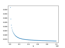
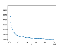
Before we proceed to the DNN theoretical counterpart, let us briefly present a single numerical test meant to support the estimates in Theorem(Part I). For more numerical tests in this sense we refer the reader to Section 5. Here, Figure 1 below depicts the evolution w.r.t. of the mean errors and for the Poisson problem (1.1), where , is the coronal cube defined in Section 5, whilst the exact solution is given by (5.4) from Section 5. The above expectations have also been approximated by Monte Carlo simulations, for more details see Section 5, more precisely Figure 7.
The second part of the main result of this paper is dedicated to the construction of a neural network approximation. In fact, in this paper we deal only with the special class of feed-forward neural networks whose activation function is given by ReLU (rectified linear unit), and such a network shall further be referred to as a ReLU DNN. The essential part of this construction is the formula (1.5). The key fact is that we choose to be already a ReLU DNN. This is the main reason for our modification of the walk on spheres algorithm with instead of the usual distance to the boundary. In addition, having some ReLU DNN approximations of the data respectively , we can use these building blocks together with some basic facts about the ReLU DNNs in conjunction with (1.8) to get the following result.
Theorem (Part II; see Theorem 3.10 for details).
Under the same context as Theorem (Part I), assume that satisfies the uniform exterior ball condition, and that we are given ReLU DNNs such that
If is chosen such that from 3.10 hold, and , then we can construct a (random) ReLU DNN such that
with
where
Furthermore, if is defective convex (see (2.15)) then we get the significant improvement
Here denotes the number of non-zero parameters in the neural network, and represent the width respectively the length of the neural network . The implicit constants depend on .
1.4 Further extensions
This paper has outlined a novel method with the potential to extend to a general principle for solving high-dimensional partial differential equations (PDEs) without encountering the curse of dimensionality. The approach is threefold:
- (i)
-
(ii)
The subsequent phase involves the rapid simulation of this stochastic process, aligning closely with the PDE solution representation. This step is harmonized with the Monte-Carlo method for approximating the solution.
-
(iii)
The final phase focuses on approximating the solution at specific points within an auxiliary grid of the domain. Following this, we employ a concentration inequality to extend this approximation to the continuous domain, thus compensating for the complexity introduced by the grid.
Such a strategy finds immediate application in the realm of parabolic PDEs solvable by diffusion processes, as discussed in [3] and [10], especially within time-dependent domains. It also applies to PDEs characterized by (sticky-)reflecting boundary conditions, in line with the frameworks established in [53] and [32].
Furthermore, this methodology opens new avenues in molecular dynamics, particularly in scenarios where the operator exhibits discontinuous coefficients, as explored in [9, 38, 36]. Another promising direction involves the extension of this approach to (sub-)Riemannian or metric measure spaces, utilizing tools as the ones in [47, 26, 51, 2, 4, 49].
1.5 Organization of the paper
In Section 2 we present the main notations, the important quantities and the main results. For the sake of readability of the paper we moved the proofs to Section 4. Section 2 in turn contains several subsections which we discuss now because they show the main approach. Subsection 2.1 details the first probabilistic representation of the solution and various types of estimates based on the annular diameter of a domain, which is a certain one dimensional characterisation of the domain. In Subsection 2.2 the walk on spheres and its modified version enters the scene and we give the main estimates on the number of steps needed to get in the proximity of the boundary for general domains. Also here we introduce the class of -defective convex domains, a class of domains for which we provide better estimates for the number of steps to the proximity of the boundary. Subsection 2.3 provides the main analysis of the modified walk-on-spheres chain stopped at a deterministic time (thus uniformly for all points in the domain and all samples) as opposed to the one in [23] which is random and very difficult to control. Here we estimate first the sup norm of where is the solution to (1.1) represented probabilistically by (2.2), whilst is given by (2.20); the estimates are given in terms of the regularity of the data, the geometry of the boundary and the parameter . If the annular diameter is finite then in fact the estimates depend only on the diameter and the annular diameter or the parameter (the convex defectivness). Furthermore, Subsection 2.4 introduces the Monte Carlo estimator (see (1.5)) for and contains the main results, namely Theorem 2.26 and Corollary 2.28. Subsection 2.5 contains the main extensions we need to deal with the walk on sphere algoritm. Fundamentally, in order to construct either (2.20) or (1.5) we need to extend the values of boundary data inside the domain and we do this under some regularity conditions.
Section 3 contains the neural network consequences of the main probabilistic results and benefits from the very careful preliminary construction of the modified walk on spheres. We should only point out the key fact that from (1.5) namely that once we replaced , and by neural networks then the function also becomes a neural network. A word is in place here about the distance function , the distance to the boundary. In the original walk on spheres, one uses for the construction of the radius of the spheres. We modified this into . The benefit is that if we have an approximation of by a neural network, we can easily construct which is already a neural network. This avoids complications which arise in [23] from the approximation of by a neural network after the Monte-Carlo estimator is constructed. The rest of the section here is judicious counting of the size of the neural network obtained for replacing and by their corresponding approximating networks.
2 The presentation of the main results
As we already discussed, this work concerns probabilistic representations and their DNN counterpart for the solution to problem
| (2.1) |
Throughout this paper, is a bounded domain in , is bounded on and is continuous on the boundary . Further regularity shall also be imposed on , and , so let us fix some notations: We say that a set is of class if its boundary can be locally represented as the graph of a function. We write to say that is continuous on . is the standard Lebesgue space with norm denoted by . For a bounded function , that is for , we shall denote by the essential sup-norm of . For and an -Hölder function for ( or Lipschitz, for ), we set .
Before we proceed, let us remark that one could also consider the anisotropic operator instead of , where is a (homogeneous) positive definite symmetric matrix, without altering the forthcoming results. This can be done mainly due to the following straightforward change of variables lemma. For completeness, we also include its short proof in the smooth case.
Lemma 2.1.
For any given a symmetric, positive-definite matrix, assume that is a classical solution to (2.1) with replaced by . If we take a matrix such that , then denoting and , we have
Proof in Subsection 4.1.
2.1 Probabilistic representation for Laplace equation and exit time estimates
We fix , to be a standard Brownian motion on which starts from zero, that is . Then, we set
and recall that the law on the path-space is precisely the law of the Brownian motion starting from .
By we denote the first hitting time of by , namely
The following result is the fundamental starting point of this work. It is standard for sufficiently regular data, but under the next assumptions we refer to [18, Theorem 6].
Theorem 2.2 ([18]).
Let and . Then there exists a unique function such that is a (weak) solution to problem (2.1). Moreover, it is given by
| (2.2) |
Let be given by
| (2.3) |
Most of the main estimates obtained in this paper are expressed in terms of the sup-norm of in the proximity of the boundary of (see e.g. (2.21)). In a following paragraph we shall explore such estimates for for domains that satisfy the uniform exterior ball condition. Before that, let us start with the following consequence of 2.2:
Corollary 2.3.
The following assertions hold for given by (2.3).
-
i)
.
-
ii)
is the solution to the Poisson problem
(2.4)
Proof in Subsection 4.1.
The annular diameter of a set in and exit time estimates
Now we explore more refined bounds for , , aiming at providing a general class of domains for which , where is a sort of annular diameter of which in particular is a one dimensional parameter that depends on . For more details, see (2.7) below for the precise definition, and 2.6 for the precise result.
The first step here in understanding the exit problem from a domain which is not necessarily convex is driven by our first model, namely the annulus defined by as
We set .
The result in this direction is the following.
Now we extend the above result to a larger class of domains, namely those that satisfy the uniform exterior ball condition. To do it in a quantitative way, we need to define first a notion of annular diameter of a set as follows:
Definition 2.1.
For a bounded domain , and , we set
| (2.6) |
with the convention . Furthermore, we set
| (2.7) |
Now for a point , taking and such that the above infimumum is attained, it is easy to see using the triangle inequality that for any and thus we get that
| (2.8) |
This is strongly related to the exterior ball condition at , since the former holds if and only if . In fact if we have the exterior ball condition with the radius of the exterior ball is , then we can choose and .
The above discussion leads to the following formal statement.
Proposition 2.5.
A bounded domain satisfies the uniform exterior ball condition if and only if . If the radius of the exterior ball is at least , we can estimate
However, for instance a ball centered at from which we remove a cone with the vertex at the center does not have a finite adiam. On the other hand, obviously, a convex bounded domain has finite adiam and in fact, this is actually equal to the diameter of the set. Indeed, one can see this by taking a tangent ball of radius and taking . Letting tend to infinity we deduce that for a convex set we actually have .
Now we can present the main estimate of this paragraph.
Proposition 2.6.
If has , then for any ,
In particular, using (2.8) and (2.7), we have
where recall that is the first exit time from and .
Proof in Subsection 4.1.
2.2 Walk-on-Spheres (WoS) and -shell estimates revisited
An important benefit of representation (2.2) is that the solution may be numerically approximated by the empirical mean of iid realizations of the random variables under expectation, thanks to the law of large numbers. One way to construct such realizations is by simulating a large number of paths of a Brownian motion that starts at and is stopped at the boundary . However, as introduced by Muller in [40], there is a much more (numerically) efficient way of constructing such realisations, based on the idea that (2.2) does not require the entire knowledge of how Brownian motion reaches . This is clearer if one considers the case , when the only information required in (2.2) is the location of Brownian motion at the hitting point of . In this subsection we shall revisit and enhance Muller’s method.
For any let denote the distance from to , or equivalently, the radius of the largest sphere centered at and contained in , that is
| (2.9) |
Clearly, is a Lipschitz function.
Recall that the standard WoS algorithm introduced by Muller [40] (see also [45], [14] or [13] for more recent developments) is based on constructing a Markov chain that steps on spheres of radius where denotes its current position. However, it is often the case, especially in practice, that merely an approximation of the distance function is available, and not the exact . This is the case, for example, if for computational reasons, is simply approximated with the (computationally cheaper) distance function to a polygonal surrogate for the domain . Another situation, which is in fact central to this study, is given in Section 3 below, when is approximated by a neural network. In both cases, is approximated by a function with a certain error. It turns out that considering the chain which walks on spheres of radius exhibits certain difficulties regarding the error analysis and also the construction of the chain itself. We do not go into more details at this point, but we refer the reader to 2.23, iii)-iv) below for a more technical explanation of these issues.
Our strategy is to solve both of the above difficulties at once, by developing from scratch the entire analysis in terms of (a modification of) , and not in terms of as it is typically done. This motivates the following concept of distance.
Definition 2.7.
Let be a bounded open set and the distance function to the boundary. Given and , a Lipschitz function is called a -distance on if
When we say that is a -distance, and if in addition then it is obvious that .
Notice that if is a -distance, then it is also a -distance for any smaller . Thus if we fix a and is a -distance, then, is also a -distance for any .
Remark 2.8.
Suppose that is a Lipschitz function such that . If and , then a simple computation yields that
is a -distance on . For example if we take , we can choose , therefore, given any , a Lipschitz approximation of , there exists which is -distance. The moral is that we can always work with a -distance with .
This example already anticipates the amenability of this to the ReLU neural networks. Indeed, the positive function is precisely the non-linear activation function and from this standpoint, if is a neural network, we can argue that becomes also a ReLU neural network. More on this in Section 3.
-WoS chain.
Let be defined (for simplicity) on the same probability space , independent and uniformly distributed, where is the sphere centered at the origin with radius . Let be the filtration generated by , where , namely
Also, let , , and be a -distance on . For each , we construct the chain recursively by
| (2.10) | ||||
| (2.11) |
Clearly, is a homogeneous Markov chain in with respect to the filtration , which starts from and has transition kernel given by
where is the normalized surface measure on ; that is, bounded and measurable. We name it an -WoS chain.
We return now to problem (2.1)
which by Theorem 2.2 admits the probabilistic representation (2.2). Further, we consider the following sequence of stopping times
| (2.12) |
Remark 2.9.
It is clear that if , i.e. is a -distance, then
The following result is a generalization of Lemma 3.4 from [23]:
Corollary 2.10.
Let be a bounded open set, , and be the solution to (2.1). Also, for bounded and measurable set
If is a -distance ( i.e. it is a -distance) then the following assertions hold:
-
i)
For all we have
where , whilst acts on with respect to the variable.
-
ii)
The mapping renders a probability measure on with density , where is the Green function associated to on . More explicitly, for we have that is proportional to
-
iii)
Let be a real valued random variable defined on , with distribution , such that is independent of . Then for all we have
(2.13)
Proof in Subsection 4.1.
Consider the -WoS chain described above, and for each let us define the required number of steps to reach the -shell of by
which is clearly an -stopping time.
The estimates to be obtained in the next subsection, and consequently the size of the DNN that we are going to construct in order to approximate the solution to (2.1), depend on how big is. The goal of this section is to provide upper bounds for , the number of steps the walk on spheres needs to get to the -shell. These estimates are first obtained for general domains, and then improved considerably for ”defective convex” domains which are introduced in 2.12, below. We provide what are, to our knowledge, the strongest estimates when compared with the currently available literature, as well as rigorous proofs that rely on the general technique of Lyapunov functions. Some of these results have some something in common with the results in [8], though the estimates in there are not clearly determined in terms of the dimension.
It is essentially known that for a general bounded domain in , the average of grows with respect to at most as (see [33, Theorem 5.4] and its subsequent discussion), hence, by Markov inequality, can be bounded by . The next result shows that, in fact, decays exponentially with respect to , and independent of the dimension .
Proposition 2.11.
Let be a bounded domain, , and be a -distance. Then for any ,
| (2.14) |
where denotes the diameter of . In particular,
Proof in Subsection 4.2.
If the domain is convex, then the average number of steps required by the WoS to reach the -shell is of order . This was shown by Muller in [40], and also reconsidered in [8]. However, it is of high importance to the present work to track an explicit constant in front of in terms of the space dimension . In this subsection we aim to clarify (the proof of) this result and extend it from convex domains to a larger class of domains, resembling the technique of Lyapunov functions from ergodic theory. More importantly, as in the case of 2.11, we are strongly interested in tail estimates for , not in its expected value. In a nutshell, the idea is to show that the square root of the distance function to is pushing the WoS chain towards the boundary at geometric speed. This is a technique meant to be easily extended for more general operators, in a further work.
The following definition settles the class of domains for which the aforementioned estimate is going to hold.
Definition 2.12.
We say that a Lipschitz bounded domain is ”-defective convex” if and
| (2.15) |
where we recall that is the distance function to the boundary , whilst .
Remark 2.13.
Recall that by [1], is convex if and only if the signed distance function is superharmonic on , where
Hence a defective convex domain as defined by (2.15) is more general than a convex domain; in fact, even if (2.15) holds (on ) with , it is not necessarily true that is convex, as explained in [1]. To give an intuition on how a defective convex domain could differ from a convex domain, imagine a ball in which is deformed into a defective convex domain by squeezing it slightly, or a straight cylinder in which is bent mildly. However, a defective convex domain can differ seriously from a convex domain, as revealed by the next two examples.
Example 2.14.
Let be an annulus of radii , namely . If for some , then is a -defective convex domain.
Proof in Subsection 4.2.
Example 2.15.
We take to be a connected, compact orientable hypersurface in , with , endowed with the Riemannian metric induced by the embedding. We denote by the principal curvatures at . The orientation is specified by a globally defined unit normal vector field . Then there exists a positive thickness , such that the tubular neighbourhood given by
| (2.16) |
is -defective convex. In fact, can be chosen explicitly in terms of the principal curvatures of .
Proof in Subsection 4.2.
Proposition 2.16.
Let be -defective convex as in (2.15). Let , and be a -distance, and consider the transition kernel of the -WoS Markov chain . If we set , then
| (2.17) |
In particular,
| (2.18) |
and if , then for any
| (2.19) |
Proof in Subsection 4.2.
Remark 2.17.
It can be shown that 2.16 still holds if condition (2.15) is satisfied merely in some strict neighbourhood of the boundary. In particular, in view of 2.15, 2.16 holds for all domains with smooth boundary, but the estimates would also depend on the thickness of the neighbourhood where condition (2.15) is fulfilled. Going even further, any bounded domain that can be uniformly approximated from inside by smooth domains enjoys, for fixed , a similar estimate with respect to and as in (2.18), with possibly depending on . This behavior is numerically confirmed by Test 1 in Section 5 for annular hypercubes, and it is going to be analyzed theoretically in a forthcoming work.
2.3 WoS stopped at deterministic time and error analysis
Throughout this subsection we assume that is the solution to problem (2.1), hence 2.2 and 2.10 are applicable. Moreover, we keep all the notations from the previous subsections. Before we proceed with the main results of this subsection, let us emphasize several aspects that are essential to this work. To make the explanation simple, assume that , that is the WoS chain is constructed using the -distance . Given , a usual way to employ WoS Markov chain in order to approximate through the representation furnished by 2.10, is to start the chain from and run it until it reaches the -shell, for some given . In other words, is usually stopped at the (random) stopping time and represented by (2.2) is then approximated with
The intuition behind is that stopping WoS chain at the -proximity of the boundary should provide a good approximation of how the Brownian motion first hits the boundary , and estimates that certify this fact are in principle well known. As discussed in the previous subsection, the number of steps required to reach the -shell is small, especially if the domain is (defective) convex, which eventually leads to a fast numerical algorithm.
From the point of view of this work (also of [23]), the fundamental inconvenience of the above stopping rule is that it depends strongly on the starting point , mainly through . In other words, although computationally efficient for estimating a single value , the above point estimate of is expected to fail at overcoming the curse of high dimensions for solving (2.1) globally in . Moreover, if one aims at constructing a (deep) neural network architecture based on the above representation, as considered in [23] and also in Section 3 below, would be the input while would give the number of layers; however, the latter should be independent of , which is obviously not the case. To deal with this architectural impediment, in [23] the authors proposed as a random time to stop the WoS chain. However, beside the measurability and the stopping time property issues for , it is still unclear, at least to us, that and that this expectation does not depend on the dimension .
Anyway, our approach is consistently different. Instead of stopping the WoS chain at a random stopping time, be it or , the idea is to stop the chain after a deterministic number of steps, say , independently of the starting point . Such a choice turns out to be feasible, and it not only avoids the above mentioned issues concerning , but it eventually provides a way to break the curse of high dimensions for solving (2.1), merely using WoS algorithm but in a global fashion. Furthermore, in terms of neural networks, this strategy would also render a way of explicitly constructing a corresponding DNN architecture, that could be easily sampled, and why not, further trained. Also, as already mentioned in 2.8, when we shall deal with neural networks in Section 3 the distance to the boundary needs to be replaced by an approximation given by a DNN, with a certain error. Therefore, in light of 2.7 and 2.8, we shall work instead with a -distance on , for some and properly chosen. Having all these in mind, the aim of this subsection is to estimate the error of approximating the solution with
| (2.20) |
for a given (deterministic) number of steps that does not depend on .
To keep the assumption on the regularity of as general as possible, the forthcoming estimates shall be obtained in terms of the function defined by (2.3) or (2.4), more precisely in terms of the behavior of near the boundary measured for each by
| (2.21) |
Though this is our primary measure of the geometry of the boundary, we can in fact refine things by defining
| (2.22) |
We include here a small result which reveals the main properties we need further on.
Proposition 2.18.
We have
| (2.23) |
For any domain and any compact ,
| (2.24) |
We will only point how one can prove this by using the observation that for any stopping time , is a bounded right-continuous supermartingale, thus converges for . As a consequence, we obtain that converges to . On the other hand, we just observe that is non-increasing in , thus by Dini’s theorem, we get the uniform convergence to .
Let us first consider the case of homogeneous boundary conditions, namely .
Proposition 2.19.
Let , , be a -distance, , and be the solution to (2.1) with . If is given by (2.20) then
| (2.25) |
In particular,
| (2.26) |
Proof in Subsection 4.3.
Let us treat now the in-homogeneous Dirichlet problem, this time taking .
Proposition 2.20.
Let , , be a -distance, be the solution to (2.1) with and . Further, for each consider that is given by (2.20) If is -Hölder on for some then
| (2.27) |
and in particular,
| (2.28) |
Proof in Subsection 4.3.
Theorem 2.21.
Let us point out that if (see (2.6) below), then involved above may be replaced by . Furthermore, when the domain is defective convex (see subsection 2.2), we can improve considerably the above error estimates with respect to the required number of WoS steps, . This can be done analogously to the proofs of 2.19 and 2.20, just by replacing the tail estimate given by 2.11 with the one provided by 2.16. Therefore, we give below the precise statement, but we skip its proof.
2.4 Monte-Carlo approximations: mean versus tail estimates
We place ourselves in the same framework as before, namely: is bounded domain, , , and is the solution to (2.1).
Further, let be a family of independent and uniformly distributed random variables on , be a -distance on for some and (see 2.7), and set:
On the same probability space as , let be iid random variables with distribution given by 2.10, ii), such that the family is independent of .
Remark 2.23.
At this point we would like to point out that estimator is different than the one employed in [23], Proposition 4.3 in several main aspects:
-
i)
The first aspect was already anticipated in the beginning of Subsection 2.3, namely instead of stopping the WoS chain at which is a random time that is difficult to handle both theoretically and practically, we simply stop it a deterministic time which is going to be chosen according to the estimates obtained in 2.26 below and its two subsequent corollaries.
-
ii)
The second aspect is that the estimator used in [23] considers iid samples drawn from , for each of the iid samples drawn from , leading to a total of samples. In contrast, requires merely samples, because and are sampled simultaneously (and independently), on the same probability space.
-
iii)
The third aspect is more subtle: In [23], the Monte Carlo estimator of type (2.29) is constructed based on a given DNN approximation of the distance to the boundary , for any prescribed error, let us say . Then, the approximation error of the solution is obtained based on the error of the Monte Carlo estimator constructed with the exact distance , and on how such an estimator varies when is replaced with . However, the latter source of error scales like , where . To compensate this explosion of error, has to be taken extremely small, and to do so, in [23] it is assumed that can be realized with complexity ; The authors show that such a complexity can indeed be attained for the case of a ball or a hypercube in , and probably can be extended to other domains with a nice geometry. Our approach is different and the key ingredient is to rely on the notion of -distance introduced in 2.7. More precisely, using 2.8 we can replace by some -distance at essentially no additional cost, and rely on the herein developed analysis for -WoS. This approach turns out to avoid the additional error of order mentioned above, in particular we shall be able to consider domains whose distance function to the boundary may be approximated by a DNN merely at a polynomial complexity with respect to the approximation error.
-
iv)
Another issue regards the construction of the WoS chain itself. Because from iii) may be strictly bigger than , for a given position , the sphere of radius might exceed , so there is a risk that the WoS chain leaves the domain . In particular, if one constructs the WoS chain based on , then in order to make the analysis rigorous the boundary data and the source should be extended also to the complement of the domain . Fortunately, this issue is completely avoided by considering -WoS chains (as it is done in this work), since by definition on .
Let us begin with the following mean estimate in :
Proposition 2.24.
Let , , and be a -distance. Then for all , and
| (2.30) |
where is the Lebegue measure on , whilst and are given by (2.20) and (2.29). In particular, the above inequality can be made more explicit by employing the estimates for obtained in 2.21 and 2.22, depending on the regularity of and .
Proof in Subsection 4.4.
Remark 2.25.
Note that as in [23], Section 4, the above error estimate depends on the volume . When scales well with the dimension (e.g. at most polynomially), then (2.30) can be employed to overcome the curse of high dimensions; in fact, if is a subset of a hypercube whose side has length less then some , then , hence, in this case, the factor improves the mean squared error exponentially with respect to . However, may also grow exponentially with respect to , and the above estimate can not be used to construct a neural network whose size scales at most polynomially with respect to the dimension. Therefore, our next (and in fact) main goal is to solve this inconvenience, by looking at tail estimates for the Monte-Carlo error; one key idea is to quantify the error using the sup-norm instead of the -norm.
Before we move forward, we recall the notion of a regular domain. We say that a bounded domain is regular if for any continuous function on the boundary, the harmonic function with the boundary condition is continuous in .
As announced in the above remark, we conclude now with the central result of this paper.
Theorem 2.26.
Keep the same framework and notations as in the beginning of this subsection. Fix a small , , a -distance, and consider and given by (2.20) and (2.29). Also, assume that and are -Hölder on for some . Then, for any compact subset , for all , and , then
| (2.31) |
where
| (2.32) |
and
| (2.33) |
If then in (2.31) the term can be replaced by and
Moreover, if we set
| (2.34) |
then we also have the estimate on the expectation of the total error in the form
| (2.35) |
As a consequence, from 2.18, for any compact set ,
| (2.36) |
For regular domains, we can take .
Furthermore, for any domain, we can replace with . Moreover, if the domain satisfies the exterior ball condition, then in (2.33) we can take and replace by .
If the domain is -defective convex, we can replace from the definition of A in (2.33) with .
Proof in Subsection 4.4.
Remark 2.27.
Note that the left hand side of (2.31) does not depend on , and if is a -distance, then it does not depend on as well. Therefore, in the right hand side of (2.31) one may take the infimum with respect to , and if is a -distance then one may also take the infimum with respect to ; but optimizing the previously obtained bounds in this way may be cumbersome. Anyway, convenient bounds can be easily obtained from particular choices of and , so let us do so in the sequel.
Let us conclude this subsection with the following consequence obtained for some convenient choices for and .
Corollary 2.28.
Let such that it satisfies the uniform exterior ball condition. Further, let and be -Hölder on for some , be a prescribed error, be a prescribed confidence, and be a -distance with and such that
| (2.37) | ||||
| Also, choose | ||||
| (2.38) | ||||
Then
| (2.39) |
whenever we choose
| (2.40) |
and
| (2.41) |
Furthermore, if is -defective convex, then can be chosen as
| (2.42) |
Proof in Subsection 4.4.
Remark 2.29.
By some simple computations, , , and from 2.28, exhibit the following asymptotic behaviors:
-
,
and if is -defective convex then
whilst if satisfies the uniform exterior ball condition then
Here, the Landau symbols tacitly depend on (the regularity of) . In particular, only in terms of the dimension , if the domain is -convex then and , whilst merely under the uniform exterior ball condition, and .
2.5 On regular extensions of the boundary data inside the domain
Recall that one assumption of the main results in the previous subsections (see e.g. 2.26) is that the boundary data can be extended as a regular function (Hölder or ) defined on the entire domain . This is required by the fact that the data needs to be evaluated at the location where the WoS chain is stopped, see (2.29), and such stopped position lies in principle in the interior of the domain . However, usually in practice, is measured (hence known) merely at the boundary . With this issue in mind, in this subsection we address the problem of extending regularly from to , in a constructive way which is also DNN-compatible.
We take to be a set of class , or , hence (see [19, sec. 14.6]) there exists a neighbourhood of such that the restriction of the distance function is of class , and the nearest point projection is of class . We have:
Lemma 2.30.
Let to be a set of class hence for any point there exist a function of class and a radius such that
We denote by . Furthermore, denoting by the ordered principal curvatures of let us take . Take to be such that on and on , . We define the extension in of the -Hölder function given on the boundary , for as:
| (2.43) |
Then is -Hölder on and
If, furthemore, the domain is of class and then is in with on and furthermore we have:
where is an explicitly computable constant in terms of , , and .
Proof in Subsection 4.5.
Remark 2.31.
One can easily provide a non-constructive -Hölder extension on of the -Hölder boundary data given on by setting .
3 DNN counterpart of the main results
Let be the rectified linear unit (ReLU) activation function, that is , . Let be a sequence of positive integers. Let and , , and set . We define the realization of the DNN by
| (3.1) |
where , , is defined coordinatewise. The weights of the ReLU DNN are the entries of . The size of denoted by is the number of non-zero weights. The width of is defined by and is the depth of denoted by . In the sequel, we only consider DNNs with ReLU activation function.
For the reader’s convenience, before we proceed to the main result of this section (see 3.10 below), we present first several technical lemmas following [15] and [52], as well as some of their consequences; all these preparatory results are meant to provide a clear and systematic way of quantifying the size of the DNN which is constructed in the forthcoming main result, namely 3.10.
The following lemma is [52, Proposition 3].
Lemma 3.1.
For every and , there exists a DNN such that
Now, we recall Lemma II.6 from [15]:
Lemma 3.2.
Let , be ReLU DNNs with the same input dimension and the same depth . Let , , be scalars. Then there exists a ReLU DNN such that
-
i)
for every ,
-
ii)
,
-
iii)
,
-
iv)
.
The following lemma is taken from [15, Lemma II.3], with the mention that the last assertion iv) brings some improvement which is relevant to our purpose; it is immediately entailed by the proof of the same [15, Lemma II.3], so we skip its justification.
Lemma 3.3.
Let and be two ReLU DNNs. Then there exists a ReLU DNN such that
-
i)
for every ,
-
iii)
,
-
iii)
,
-
iv)
.
The next lemma is essentially [15, Lemma II.4]. As in the case of the previous lemma, assertion iv) comes with a slight modification of the original result, which can be immediately deduced from the proof of [15, Lemma II.4].
Lemma 3.4.
Let be a ReLU DNN such that . Then there exists a second ReLU DNN such that
-
i)
for all ,
-
ii)
,
-
iii)
,
-
iv)
.
As a direct consequence of 3.1, 3.3, 3.4, and [15, Lemma II.5], one gets the following approximation result for products of scalar ReLU DNN:
Corollary 3.5.
Let be two ReLU DNNs, be a bounded subset, and let be given by 3.1 for and . Then there exists a ReLU DNN such that
-
i)
for every ,
-
ii)
-
iii)
.
The following two lemmas are going to be employed later in order to quantify the size of one generic step of the WoS chain given by (2.10)-(2.11), regarded as an action of a ReLU DNN.
Lemma 3.6.
Let be a ReLU DNN and be a vector. Then there exists a ReLU DNN such that
-
i)
for all ,
-
ii)
,
-
iii)
,
-
iv)
.
Proof in Subsection 4.5.
Corollary 3.7.
Let be a ReLU DNN and be a sequence of vectors. Then there exist ReLU DNNs , such that for every
-
i)
and for all , where is the one constructed in 3.6,
-
ii)
,
-
iii)
,
-
iv)
.
We end this first paragraph by a ReLU DNN extension of a Hölder continuous boundary data to the entire domain .
Corollary 3.8.
Let to be a set of class and be -Hölder on . For and as defined in Lemma 2.30 we assume that for every , there exist ReLU DNNs , , and such that
With the one given in 2.30, set
If is the -Hölder extension in of the boundary data given by (2.43), then there exists a ReLU DNN such that
-
i)
-
ii)
.
Proof in Subsection 4.5.
3.1 DNN approximations for solutions to problem (2.31)
We are now ready to present the DNN byproduct of 2.26, in fact of 2.28. First, let us state that the -WoS chain given by (2.10)-(2.11) renders a ReLU DNN as soon as is a ReLU DNN; this follows from a simple corroboration of 3.6 and 3.7, so we skip its formal proof.
Corollary 3.9.
Suppose that is a ReLU DNN on the bounded set such that , where recall that specified by (2.9) is the distance function to the boundary of . Further, let and be the -WoS chain at step given by . Then for each there exists a ReLU DNN defined on and denoted by such that
-
i)
for all ,
-
ii)
,
-
iii)
,
-
iv)
.
The main result of this section is the following, proving that ReLU DNNs can approximate the solution to problem (2.31) without the curse of dimensions.
Theorem 3.10.
The statement requires a detailed context, so let us label the assumption and the conclusion separately.
Assumption: Let be a bounded domain satisfying the uniform exterior ball condition, and be -Hölder functions on for some , and be the solution to (2.31), as in 2.2. Let be ReLU DNNs such that
and set Also, let be the ReLU DNN given by 3.1.
Further, let be a prescribed error, be a prescribed confidence, and consider the following assumptions on the parameters :
-
a.1)
,
-
a.2)
,
-
a.3)
, so that, by 2.8, is a -distance if we choose ,
-
a.4)
and ,
where is specified below.
Further, consider the iid pairs on , as in the beginning of Subsection 2.4, and
| (3.2) |
Let us choose
| (3.3) | ||||
| (3.4) |
where .
Furthermore, if is -defective convex then can be chose such that
Conclusion: Under the above assumption and keeping the same notations, there exits a measurable function such that
-
c.1)
is a ReLU DNN for each , and
-
c.2)
For each we have that
In particular,
where
and the tacit constant depends on .
Furthermore, if is -defective convex then if holds then
.
Proof in Subsection 4.5.
We end the exposition of the main results with the remark that it is sufficient to prescribe the Dirichlet data merely on (not necessarily extended to ), as expressed by the following direct consequence of 3.8.
4 Proofs of the main results
4.1 Proofs for Subsection 2.1
Proof of 2.1.
Let . Then and
Thus we need to determine such that . We know that there exists a rotation matrix (hence ) such that . Since is positive definite we have for . Then we have:
| (4.1) |
We denote and observe that (4.1) can be rewritten as . We can now take . Thus . ∎
Proof of 2.3.
The second assertion follows directly from 2.2 and from classical regularity theory for Poisson equation, so let us prove the first one. To this end, note that without loss of generality we may assume that , so by Ito’s formula we get that is a martingale and
∎
Proof of 2.10.
i). Using 2.9 we have that,
where the second equality follows by the strong Markov and the scaling properties of Brownian motion, whilst the last equality follows from the fact that the law of under and the law of under are the same. Therefore, the statement follows by 2.2.
ii). The claim follows from the fact that , where solves
for all .
iii). We use conditional expectation, namely for every
where for the last equality we used that has distribution and is independent of . ∎
Proof of 2.4.
Recall that , where is given by (2.3). The idea is to explicitly solve for in radial form as
which is explicitly solved as
Now, if we start from a point we can use the intermediate value theorem to obtain first that
for some point . Therefore our task now is to estimate the above derivative, which we can compute explicitly as
To estimate this in a transparent way we set and for . In these new notations we have
Now, it is an elementary matter that for two functions which are differentiable on (and non-vanishing), we can find a point such that
Using this fact for , and we argue that for some point we have
As a function of the above function is increasing, thus we have
| (4.2) |
Therefore in order to control it suffices to control the absolute values of the two bounds above. The right hand side bound is easy because for any , thus we obtain that
| (4.3) |
The left hand side of (4.2) in absolute value is bounded by
| (4.4) |
where we go back to the fact that and in the second line we used that because for . Thus combining (4.3) and (4.4) we get that
which is our claim. ∎
4.2 Proofs for Subsection 2.2
Proof of 2.11.
The proof goes through several steps.
The first step observes the following two basic facts which can be easily checked by direct computations. On the ball of radius centered at we have
| (4.5) |
and
| (4.6) |
The second step consists in proving some estimates for the exit time of the Brownian motion from the ball of radius and centered at . Denote by this exit time for the Brownian motion started at the origin. Then
| (4.7) |
and
| (4.8) |
The proofs of (4.7) and (4.8) are based on the previous step. For example, using (4.5) we learn that for and this combined with Itô’s formula means that is a supermartingale. In particular, stopping it at time , we obtain that
from which we deduce (4.7).
With these two steps at hand we can move to proving the actual result. To proceed, we take the iid sequence of uniform random variables on the unit sphere in which drives the walk on spheres. Now set to denote the number of steps to the -shell for the walk on spheres using the random variables . Notice that for a fixed point , in distribution sense, have the same distribution for all . Also, set the point on the sphere of radius determined by the first step of the walk on spheres determined by . The key now is the fact that
| (4.9) |
The intuitive explanation of this is rather simple, the walk on spheres starts with the first step. If we land in the -shell we stop. Otherwise we have to start again but this time we have already used the random variable and thus we have to base our remaining walk on spheres using .
Using now (4.9) we can write that
| (4.10) |
where we used conditioning with respect to the first random variable .
Now we are going to use a such that
where is the first exit time of the Brownian motion from the ball of radius starting at . This is the place where we can use the estimate (4.8) to show that is sufficient to guarantee the above estimate. Notice the key point here, namely the fact that has the same distribution as where is the Brownian motion started at and denotes the exit time of the Brownian motion from the ball of radius .
Thus now we use this to argue that
| (4.11) |
Now repeating this one more step using the new starting point we will get
Repeating this we finally obtain that
| (4.12) |
Here we use and . To finish the proof, we need to estimate now the right hand side in (4.12). To do this we enclose the domain in the ball of radius centered at and now use (4.7) with to get that
Finally, using that for and choosing , we obtain (2.14).
The second inequality of the statement is obtained based on the first estimate and Markov inequality:
∎
Proof of 2.14.
The -defectiv convexity condition for this region amounts to the inequality:
where we used the fact that the distance function is Lipschitz, hence one can integrate by parts and discard the boundary terms due to the fact that .
We use the fact that on and the function is in fact smooth and we integrate by parts on each region to obtain that the left hand side above becomes:
where we used spherical coordinates on the boundary and denoted by prime the derivative in the radial direction. Also, the is well defined, in a classical sense, on except for the set of measure zero that in spherical coordinates is given by . Noting that:
we have for all and for all , hence the -defective convexity condition amounts to the inequality:
which (taking into account that ) is satisfied if for instance . ∎
Proof of 2.15.
Arguing similarly as in the previous example, the -defective convexity condition becomes:
| (4.13) |
where is well-defined, in a classical sense, except on the set of measure zero . We also denote respectively .
We recall (see for instance, [19], Lemma , p. 355) that
hence we have:
thus the condition (2.15) holds for suitably small . ∎
Proof of 2.16.
We split the proof in two steps.
Step I (Regularization). Let for each , where is such that . Further, let be a (smooth) mollifier on such that , and set , . In particular,
| (4.14) |
Now let us consider that we extend from to by setting on , and set
We claim that
-
i)
on for all and .
-
ii)
on for all and .
To prove the claim, note first that by a simple calculation we get
hence ii) follows from i) and the fact that . So, it remains to prove the first assertion of the claim: Let , and proceed with integration by parts and Fubini’s theorem as follows
| so, by (4.14) and then using (2.15) we can continue with | ||||
which proves i) and hence the entire claim.
Now, by Ito’s formula in corroboration with the claim proved above yield:
| (4.15) |
Step II (Passing to the limit in (4.15)). The next step is to let and then in (4.15). To this end, note that because , we have
-
iii)
uniformly on ,
-
iv)
a.e. and boundedly on .
In particular, because for large enough and , we have that
-
v)
boundedly on , for each .
We are now in the position to let in (4.15) to get that for
where we have used that a.e. The fact that , follows from two basic facts. On one hand, is -Lipschitz so . On the other hand, from Lipschitz conditions and Rademacher theorem, is differentiable almost everywhere. If is a point where is differentiable, and such that , and , then it is easy to see that the derivative of in the direction is constant , thus the claim.
4.3 Proofs for Subsection 2.3
Proof of 2.19.
Further, we need the following lemma:
Lemma 4.1.
Let , , be a -distance, , and be the corresponding -WoS chain. If is a finite stopping times such that . If is -Hölder on for some then
If then
Proof.
It is easy to see that for , is a bounded martingale, hence
By employing the martingale problem for the Markov chain , we get that for any finite stopping time , hence and therefore
Suppose now that . Then, by the martingale problem we deduce
On the other hand, by Itô’s formula
hence
∎
Proof of 2.20.
4.4 Proofs for Subsection 2.4
Before proving the main result, 2.26, we need several preliminary Lemmas.
Lemma 4.2.
Let and . If and are -Hölder for some , and , then
for all almost surely. In particular,
Proof.
Clearly, it is sufficient to prove the estimate for , independently of , . To this end, since is Lipschitz
Therefore,
∎
The next lemma is the well-known Hoeffding’s inequality:
Lemma 4.3.
Suppose that are iid real random variables such that for all . Then for all and
Using Hoeffding’s inequality we immediately get the following estimate.
Corollary 4.4.
For all , and we have
Proof.
Finally, we are in the position to prove the main theorem.
Proof of 2.26.
First of all, assume without loss of generality that , and for each consider the grid
For such that we set
Note that {fleqn}
where the last inequality follows from 4.2 and by the fact that
Consequently, by setting
and using union bound inequality we have
In the case of , we only need to use the second part of 2.21, the rest of the argument being the same.
The assertions about the particular domains are clear.
For the statement about the expectation stated in (2.35), we only have to involve the following Lemma.
Lemma 4.5.
If is a non-negative random variable with the property that there exist constants and such that
| (4.17) |
then
Proof.
Start with and write
Optimizing over , yields the optimum point as
which in turn yields
This concludes the estimate. ∎
The rest of the statements in the theorem are straightforward now.
∎
Proof of 2.28.
Note that since is a -distance, it is also a -distance since .
Now, using (2.38) we get that
Also, because , by 2.6 we have that . Therefore, since is given by (2.37) and using that , we get that
Now, if is as in (2.41), then
Furthermore, if is -defective convex and is chosen as in (2.42), we have that
All the choices above ensure that from 2.26 satisfies
Taking into account the above inequality and the estimate (2.31), it is a dircet check to see that the right hand side of (2.31) is less than if satisfies (3.3), which concludes the proof. ∎
4.5 Proofs for Subsection 2.5
Proof of 2.30.
We have:
For the second part, we know that if of class and and thus . Using the definition of we have
| respectively | ||||
Taking into account that and we have:
For any point let and denote respectively the unit exterior normal to at the point and the tangent hyperspace to at . By a rotation of coordinates we can assume that the coordinate lies in the direction . In some neighbourhood of , is given by where , and . The eigenvalues of the matrix denoted are then the principal curvatures of at . By a further rotation of coordinates we can assume that the axes lie along principal directions corresponding to at .
The Hessian matrix with respect to the principal coordinate system at described above is given by
As noted in the proof of Lemma in [19] the maximal radius of the interior ball that can be associated to each point on the boundary, is bounded from below by a certain and we have that bounds the principal curvatures, hence our choice of as .
The unit exterior normal vector at a point is given by
Hence with respect to the principal coordinate system at we have:
| (4.18) |
We note that for each there exists a unique such that . We have:
| (4.19) |
As pointed in the proof of Lemma in [19] we have . Differentiating the i-th coordinate of (4.19) with respect to we get:
| (4.20) |
Furthermore, differentiating (4.20) with respect to we get:
| (4.21) |
As noted in the proof of Lemma in [19] we have that in terms of a principal coordinate system at as chosen before
| (4.22) |
and,
| (4.23) |
hence
| (4.24) |
hence
where we estimated because due to the cut-off function we only need to estimate in the neighbourhood of the boundary.
∎
Proof of 3.6.
Proof of 3.8.
We first note that
Therefore, by the triangle inequality we get
Proof of 3.10.
i) The fact that can be realized, for each , as a ReLU DNN, denoted in the statement by , is a direct consequence of 3.9, 3.5, 3.3, and 3.2.
Next, let be given by (2.29) and consider the modification of by replacing and with and , namely
Then using assumption we can easily deduce that . Therefore,
where the last inequality follows from assumptions , . Consequently,
so, we can employ 2.28 to conclude the first assertion.
Let us proceed at proving ii). First of all, note that
| (4.25) |
Further, for each , by 3.3 we get
| and since has the same size as , we can continue with | ||||
| (4.26) | ||||
| (4.28) | ||||
| (4.29) |
Finally, corroborating (4.25) with (4.29) and by applying 3.2, we obtain that for each
and by assumption we deduce that
where the tacit constant depends on .
In particular,
where
and the tacit constant depends on .
Now, if is -defective convex, then
where is as above and the tacit constant depends on . ∎
5 Numerical results
Throughout this section we numerically test some key theoretical results obtained in this paper. In order to take advantage of the highly parallelizable properties of the proposed Monte Carlo methods, we have implemented the algorithms using GPU parallel computing within the PyTorch framework.
Concretely, we consider two types of domains, namely:
which are illustrated by Figure 2 for the case .
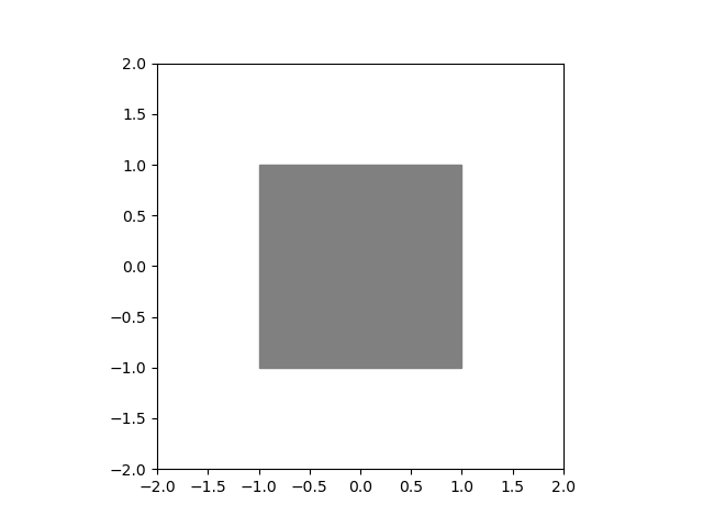
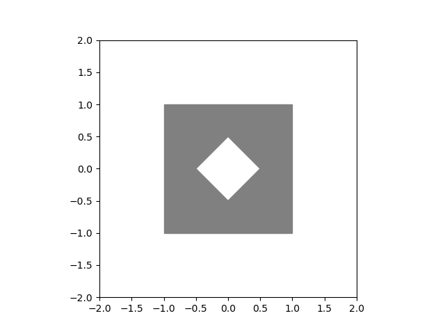
We have performed the following numerical tests by:
Test 1. Here we numerically verify the estimate (2.18), namely that
| (5.1) |
by fixing and varying and for both and . Note that is -defective convex since it is in fact convex, so (5.1) is valid with by 2.16. Furthermore, for this test, the WoS is constructed with the exact distance to the boundary, so we shall take . On the other hand, is not defective convex since if we denote the boundary corner by , then is unbounded on the cone , hence (2.15) can not hold. Nevertheless, for fixed we speculated in 2.17 that a similar asymptotic behavior as in (5.1) still holds with respect to and ; this is numerically tested in Figure 5(b) below.
Let us introduce the notations
so that the inequality to be tested becomes
| (5.2) |
We obtained the following results:
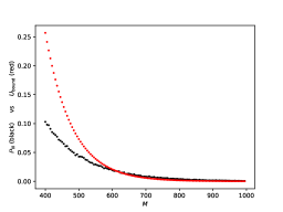
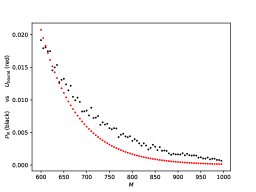
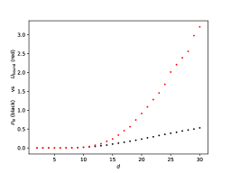
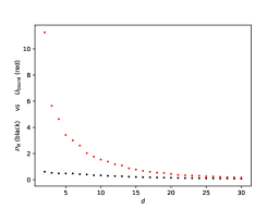
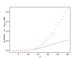
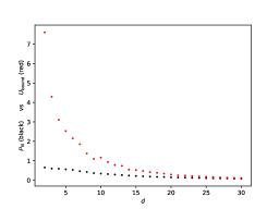
Comments on Test 1.
-
The numerical results depicted in Figure 3 and Figure 4 validate the upper bound (5.2). Note that in Figure 3(b), namely for large values of , inequality (5.2) becomes quite sharp, yet slightly reversed; the apparent reversed inequality is just a consequence of the Monte Carlo error that appears in the approximation corresponding to Monte Carlo samples.
-
Finally, recall that our main estimates obtained in the previous sections in the case of defective convex domains require . This requirement is suggested also by comparing Figure 4(a) versus Figure 4(b) as well as Figure 5(a) versus Figure 5(b); in Figure 4(b) and Figure 5(b) we have chosen instead of only because in the latter case it is harder to nicely visualize the numerical results.
Test 2. Here the goal is to test the approximation of the solution to (1.1) by simulating its Monte Carlo estimator (1.5). For simplicity we take the source term , hence we deal with
| (5.3) |
In order to validate the numerical results, we consider a particular explicit solution to (5.3), namely
| (5.4) | ||||
| (5.5) |
Further, we need to introduce some notations. For and independent and uniformly distributed on , we introduce the notations
| where are iid copies of , independent of , | ||||
where are independent copies of . In particular, by the law of large numbers we immediately have
| (5.6) |
whilst by a similar argument as in [5, Lemma 4.3] one can show that
| (5.7) |
The aim of this test is to numerically validate the approximation by computing the mean errors and . To this end, justified by (5.6) and (5.7), we shall simulate and for large, e.g. or . In order to reduce the computational burden, the value of is going to be taken relatively small, e.g. or . However, we point out that choosing a small value for shall not alter the reliability of the Monte Carlo estimate, mainly due to the fact that one can show that the distribution of is concentrated.
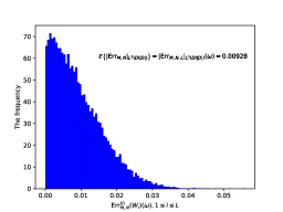
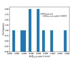
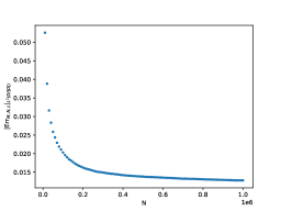
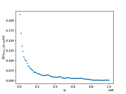
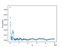
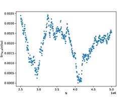
Comments on Test 2.
-
The numerical tests depicted by Figure 7 for the Poisson problem (5.3) for and confirm that the errors and , approximated by (5.6) and (5.7) respectively, are decreasing to a small value as the number of WoS trajectories increases. The limit error attained when goes to infinity is not zero as it depends on , but it decreases to zero as the latter parameter is also increased to infinity. This is discussed in the next comment.
-
Concerning the dependence of and with respect to , our numerical tests revealed that on the one hand the choice of required in 2.26 or 2.28 is quite optimal, and on the other hand that the value of can be in fact taken much smaller than the one required in the same theoretical results. As a consequence suggested by this numerical evidence, one could expect that the width of the DNNs provided by 3.10 can be significantly reduced.
-
Finally, let us emphasize that the numerical results obtained during Test 2 are conducted for the domain which is nor defective convex, neither satisfies the uniform exterior ball condition, hence the test turned out to be successful even on a worse domain geometry.
Acknowledgements. Lucian Beznea and Oana Lupascu-Stamate were supported by a grant of the Ministry of Research, Innovation and Digitization, CNCS - UEFISCDI, project number PN-III-P4-PCE-2021-0921, within PNCDI III. Iulian Cimpean acknowledges support from the project PN-III-P1-1.1-PD-2019-0780, within PNCDI III. The work of Arghir Zarnescu has been partially supported by the Basque Government through the BERC 2022-2025 program and by the Spanish State Research Agency through BCAM Severo Ochoa excellence accreditation Severo Ochoa CEX2021-00114 and through project PID2020-114189RB-I00 funded by Agencia Estatal de Investigación (PID2020-114189RB-I00 / AEI / 10.13039/501100011033).
References
- [1] D.H. Armitage and Ü. Kuran. The convexity of a domain and the superharmonicity of the signed distance function. Proceedings of the Amer. Math. Soc., 93(4):598–600, 1985.
- [2] Marc Arnaudon and Xue-Mei Li. Reflected Brownian motion: selection, approximation and linearization. Electronic Journal of Probability, 22(none):1 – 55, 2017.
- [3] Vlad Bally and Denis Talay. The law of the euler scheme for stochastic differential equations: I. convergence rate of the distribution function. Probability Theory and Related Fields, 104, 07 1994.
- [4] Fabrice Baudoin. Stochastic analysis on sub-Riemannian manifolds with transverse symmetries. The Annals of Probability, 45(1):56 – 81, 2017.
- [5] Christian Beck, Sebastian Becker, Philipp Grohs, Nor Jaafari, and Arnulf Jentzen. Solving the Kolmogorov PDE by means of Deep learning. J. Sci. Comput., 88(3), sep 2021.
- [6] Christian Beck, Martin Hutzenthaler, Arnulf Jentzen, and Benno Kuckuck. An overview on deep learning-based approximation methods for partial differential equations. Discrete and Continuous Dynamical Systems - B, 28(6):3697–3746, 2023.
- [7] Lucian Beznea and Andrei-George Oprina. Nonlinear pdes and measure-valued branching type processes. Journal of Mathematical Analysis and Applications, 384(1):16–32, 2011. Special Issue on Stochastic PDEs in Fluid Dynamics, Particle Physics and Statistical Mechanics.
- [8] I. Binder and M. Braverman. The rate of convergence of the walk on spheres algorithm. Geometric and Functional Analysis, 22(3):558–587, 2012.
- [9] Mireille Bossy, Nicolas Champagnat, Sylvain Maire, and Denis Talay. Probabilistic interpretation and random walk on spheres algorithms for the poisson-boltzmann equation in molecular dynamics. ESAIM: Mathematical Modelling and Numerical Analysis, 44(5):997–1048, 2010.
- [10] Krzysztof Burdzy, Zhen-Qing Chen, and John Sylvester. The heat equation and reflected Brownian motion in time-dependent domains. The Annals of Probability, 32(1B):775 – 804, 2004.
- [11] Patrick Cheridito, H. Soner, Nizar Touzi, and Nicolas Victoir. Second order backward stochastic differential equations and fully non-linear parabolic pdes. 10 2005.
- [12] G. Cybenko. Approximation by superpositions of a sigmoidal function. Mathematics of Control, Signals and Systems, 2(4):303–314, 1989.
- [13] M. Deaconu, S. Herrmann, and S. Maire. The walk on moving spheres: A new tool for simulating brownian motion’s exit time from a domain. Mathematics and Computers in Simulation, 135:28–38, 2017. Special Issue: 9th IMACS Seminar on Monte Carlo Methods.
- [14] Madalina Deaconu and Antoine Lejay. A random walk on rectangles algorithm. Methodology And Computing In Applied Probability, 8:135–151, 03 2006.
- [15] D. Elbrächter, D. Perekrestenko, P. Grohs, and H. Bölcskei. Deep neural network approximation theory. IEEE Transactions on Information Theory, 67(5):2581–2623, 2021.
- [16] Arash Fahim, Nizar Touzi, and Xavier Warin. A probabilistic numerical method for fully nonlinear parabolic PDEs. The Annals of Applied Probability, 21(4):1322 – 1364, 2011.
- [17] J. F. Le Gall. Spatial branching processes, random snakes, and partial differential equations. 1999.
- [18] W.D. Gerhard. The probabilistic solution of the Dirichlet problem for with singular coefficients. Journal of Theoretical Probability, 5(3):503–520, 1992.
- [19] D. Gilbarg and N.S. Trudinger. Elliptic Partial Differential Equations of Second Order. Springer, 2001.
- [20] Emmanuel Gobet. Monte-Carlo methods and stochastic processes: from linear to non-linear. Chapman and Hall/CRC, 2016.
- [21] Lukas Gonon, Philipp Grohs, Arnulf Jentzen, David Kofler, and David Šiška. Uniform error estimates for artificial neural network approximations for heat equations. IMA Journal of Numerical Analysis, 42(3):1991–2054, 2022.
- [22] Lukas Gonon, Philipp Grohs, Arnulf Jentzen, David Kofler, and David Šiška. Uniform error estimates for artificial neural network approximations for heat equations. IMA Journal of Numerical Analysis, 42(3):1991–2054, 2021.
- [23] P. Grohs and L. Herrmann. Deep neural network approximation for high-dimensional elliptic PDEs with boundary conditions. IMA Journal of Numerical Analysis, 42(3):2055–2082, 05 2021.
- [24] Gerald Trutnau Haesung Lee, Wilhelm Stannat. Analytic theory of Itô-stochastic differential equations with non-smooth coefficients. arxix, (none), 2022.
- [25] J. Han, A. Jentzen, and E. Weinan. Solving high-dimensional partial differential equations using deep learning. Proceedings of the National Academy of Sciences, 115(34):8505–8510, 2018.
- [26] Elton P Hsu. Stochastic analysis on manifolds. Number 38. American Mathematical Soc., 2002.
- [27] Martin Hutzenthaler, Arnulf Jentzen, and Thomas Kruse. Overcoming the curse of dimensionality in the numerical approximation of parabolic partial differential equations with gradient-dependent nonlinearities. Foundations of Computational Mathematics, page 905–966, 2022.
- [28] Martin Hutzenthaler, Arnulf Jentzen, Thomas Kruse, Tuan Anh Nguyen, and Philippe von Wurstemberger. Overcoming the curse of dimensionality in the numerical approximation of semilinear parabolic partial differential equations. Proceedings of the Royal Society A, 476(2244):20190630, 2020.
- [29] Martin Hutzenthaler, Arnulf Jentzen, Thomas Kruse, and Tuan Nguyen. A proof that rectified deep neural networks overcome the curse of dimensionality in the numerical approximation of semilinear heat equations. SN Partial Differential Equations and Applications, 1, 04 2020.
- [30] Martin Hutzenthaler, Arnulf Jentzen, and von Wurstemberger Wurstemberger. Overcoming the curse of dimensionality in the approximative pricing of financial derivatives with default risks. Electronic Journal of Probability, 25(none):1 – 73, 2020.
- [31] A. Jentzen, D. Salimova, and T. Welti. A proof that deep artificial neural networks overcome the curse of dimensionality in the numerical approximation of kolmogorov partial differential equations with constant diffusion and nonlinear drift coefficients. Communications in Mathematical Sciences, 19(5):1167–1205, 2021.
- [32] Vitalii Konarovskyi, Victor Marx, and Max von Renesse. Spectral gap estimates for Brownian motion on domains with sticky-reflecting boundary diffusion. arXiv e-prints, page arXiv:2106.00080, May 2021.
- [33] A.E. Kyprianou, A.Osojnik, and T. Shardlow. Unbiased ‘walk-on-spheres’ monte carlo methods for the fractional laplacian. IMA Journal of Numerical Analysis, 38, 09 2017.
- [34] I.E. Lagaris, A. Likas, and D.I. Fotiadis. Artificial neural networks for solving ordinary and partial differential equations. IEEE transactions on neural networks, 9(5):987–1000, 1998.
- [35] I.E Lagaris, A.C. Likas, and D.G. Papageorgiou. Neural-network methods for boundary value problems with irregular boundaries. IEEE Transactions on Neural Networks, 11(5):1041–1049, 2000.
- [36] Antoine Lejay and Sylvain Maire. New monte carlo schemes for simulating diffusions in discontinuous media. Journal of computational and applied mathematics, 245:97–116, 2013.
- [37] A. Malek and R. Shekari Beidokhti. Numerical solution for high order differential equations using a hybrid neural network—optimization method. Applied Mathematics and Computation, 183(1):260–271, 2006.
- [38] Miguel Martinez and Denis Talay. One-dimensional parabolic diffraction equations: pointwise estimates and discretization of related stochastic differential equations with weighted local times. Electronic Journal of Probability, 17:1–30, 2012.
- [39] T. Marwah, Z.C. Lipton, and A. Risteski. Parametric complexity bounds for approximating pdes with neural networks. In M. Ranzato, A. Beygelzimer, Y. Dauphin, P.S. Liang, and J. Wortman Vaughan, editors, Advances in Neural Information Processing Systems, volume 34, pages 15044–15055. Curran Associates, Inc., 2021.
- [40] M.E. Muller. Some continuous monte carlo methods for the dirichlet problem. The Annals of Mathematical Statistics, pages 569–589, 1956.
- [41] Etienne Pardoux and Shanjian Tang. Forward-backward stochastic differential equations and quasilinear parabolic pdes. Probability Theory and Related Fields, 114(2):123–150, 1999.
- [42] A. Pinkus. Approximation theory of the mlp model in neural networks. Acta Numerica, 8:143–195, 1999.
- [43] M. Raissi, P. Perdikaris, and G. Karniadakis. Physics-informed neural networks: A deep learning framework for solving forward and inverse problems involving nonlinear partial differential equations. Journal of Computational Physics, 378:686–707, 2019.
- [44] K.K. SABELFELD and D. TALAY. Integral formulation of the boundary value problems and the method of random walk on spheres. Monte Carlo Methods and Applications, 1(1):1–34, 1995.
- [45] K.K. Sabelfeld and D. Talay. Integral formulation of the boundary value problems and the method of random walk on spheres. Monte Carlo Methods and Applications, 1(1):1–34, 1995.
- [46] J. Sirignano and K. Spiliopoulos. DGM: A deep learning algorithm for solving partial differential equations. Journal of Computational Physics, 375:1339–1364, 2018.
- [47] Daniel W Stroock. An introduction to the analysis of paths on a Riemannian manifold. Number 74. American Mathematical Soc., 2000.
- [48] Denis Talay and Luciano Tubaro. Expansion of the global error for numerical schemes solving stochastic differential equations. Stochastic Analysis and Applications, 8(4):483–509, 1990.
- [49] Anton Thalmaier and James Thompson. Exponential integrability and exit times of diffusions on sub-riemannian and metric measure spaces. Bernoulli, 26(3):2202–2225, 2020.
- [50] N. Valenzuela. A new approach for the fractional laplacian via deep neural networks. arXiv preprint arXiv:2205.05229, 2022.
- [51] Max-K von Renesse and Karl-Theodor Sturm. Transport inequalities, gradient estimates, entropy and ricci curvature. Communications on pure and applied mathematics, 58(7):923–940, 2005.
- [52] D. Yarotsky. Error bounds for approximations with deep relu networks. Neural Networks, 94:103–114, 2017.
- [53] Yijing Zhou, Wei Cai, and Elton Hsu. Computation of local time of reflecting brownian motion and probabilistic representation of the neumann problem. Communications in Mathematical Sciences, 15, 02 2015.