Transition from insulating to conducting states in the bilayer Hubbard model by perpendicular quench field

Abstract

A many-body quantum system with different parameters may support two distinct quantum states in the same energy shell. It allows the dynamical transition from the ground state of pre-quench Hamiltonian to a steady state of post-quench one. We study the dynamical response of the ground states of a two-layer half-filled Hubbard model to a perpendicular electric field. We show that the steady state is conducting state when the field is resonant to the on-site repulsion, while the initial state is a Mott-insulating state. In addition, two layers exhibit the same conducting behavior due to the formation of the long-lived dopings, which are manifested by the performance of the charge fluctuation. The key to achieving this dynamic transition is the cooperation between on-site interaction and the resonant field rather than the role of either. Our finding provides an alternative mechanism for field-induced conductivity in a strongly correlated system.

I Introduction

Understanding the static and dynamical properties of strongly correlated quantum systems poses a major challenge in both theory and experiment Dagotto (1994); Georges et al. (1996); Yeshurun et al. (1996); Dukelsky et al. (2004); Basov and Timusk (2005); Bloch et al. (2008); Aoki et al. (2014). Although the presence of strong quantum correlations often precludes intuitive models, the interplay between particle-particle interaction and kinetic energy gives rise to novel effects including the magnetism and superconductivity Auerbach (1994); Sierra and Martín-Delgado (1997); Giamarchi et al. (2016). The Hubbard model provides a minimal paradigm for studying these properties and, as such, is attracting the attention of theoreticians from many different corners of condensed matter Hubbard and Flowers (1964); Fisher et al. (1989); Yang (1989); Georges et al. (1996); Lee et al. (2006); Sachdev (2011); Keimer et al. (2015); Zhang and Song (2021); Xie et al. (2023). Recent years have seen a significant progress in simulating quantum many-body physics with ultracold atoms that are well isolated from the environment and therefore evolve under their intrinsic quantum dynamics Giorgini et al. (2008); Bloch et al. (2008); Randeria et al. (2012); Christian and Immanuel (2017). In particular, ultracold fermionic atoms in an optical lattice can be used to realize the Hubbard model Köhl et al. (2005); Jördens et al. (2008); Schneider et al. (2008); Esslinger (2010); Taie et al. (2012); Hart et al. (2015); Duarte et al. (2015); Cocchi et al. (2016); Hartke et al. (2020). However, most real materials possess rather complex lattice structures, which can be approximated as a system of coupled layers. Fortunately, a bilayer Fermi–Hubbard model can be realized through a highly stable vertical superlattice González-Tudela and Cirac (2019); Koepsell et al. (2020); Gall et al. (2021); Meng et al. (2021), which provides a platform to study the basic property and enlarge our understanding of the multi-layer interacting system.

Driven by the advances of high-resolution microscopy, the theory describing the various quantum phase transitions has advanced remarkably in the context of interacting many-body quantum systems at equilibrium. However, the behavior of such systems is far less understood when it comes to the non-equilibrium regime, whose relevance has rapidly grown triggered by the significant experimental progress. Examples of systems that offer a large degree of control such as ultracold atoms in optical lattices Greiner et al. (2002); Bloch et al. (2008); Estève et al. (2008); Schneider et al. (2008); Bakr W. et al. (2010); Abanin et al. (2019), trapped ions Albiez et al. (2005); Schumm et al. (2005); Hofferberth et al. (2007); Bakr W. et al. (2010); Blatt and Roos (2012), superconducting qubits Roushan et al. (2017); Xu et al. (2018), as well as nuclear and electron spins associated with impurity atoms in diamond Doherty et al. (2013); Schirhagl et al. (2013). The tunability and long coherence times of these systems, along with the ability to prepare highly non-equilibrium states, enable one to probe quantum dynamics and thermalization in closed systems Abanin et al. (2019). Hence, it seems very timely to investigate the non-equilibrium behavior of the bilayer Hubbard system and unravel the potential exotic behavior.

The bilayer Hubbard model served as a paradigm to study band to Mott insulator crossover Kancharla and Okamoto (2007); Gall et al. (2021). In the large $U$ limit, whether the ground state is in a planar antiferromagnetically ordered Mott insulating phase or a band insulating phase is fully determined by the ratio of the inter-and intra-layer coupling. But no matter what phase the system is in, its ground state is non-conductive. In this work, we propose a way to realize the conductivity of the two-layer system through non-equilibrium dynamics. To this end, we first prepare the system into a Mott insulator phase with a strong antiferromagnetic correlation. Then we switch on a resonant perpendicular electric field such that the single-occupied Mott insulating states and non-ferromagnetic state doped with doublons and holes hybridize in the same energy shell. This guarantees the significant charge fluctuation of the low-energy eigenstates of the post-quench Hamiltonian since the conducting proportion overwhelms the insulating ratio. Furthermore, these states reside in the low-lying sector protected by the energy gap. This keeps the two layers with dopings for a long time providing a platform to facilitate the mobility of the particles in each layer under the non-ferromagnetic background. Accordingly, the evolved state driven by the post-quench Hamiltonian can hardly return to the initial insulating state with zero charge fluctuation. Correspondingly, the system enters into a non-equilibrium conducting phase featured by the large charge fluctuation. The key ingredient of our proposal is the formation of the long-lived dopings in each layer arising from the cooperation between the on-site interaction and the resonant electric field. It is hoped that these results can inspire further studies on the non-equilibrium bilayer even multi-layer interacting system.

The remainder of the paper is structured as follows: In Sec. II, we introduce the bilayer Hubbard model subjected to a perpendicular electric field. Aiding by the symmetries of the considered system, the role of the external field is elucidated in the absence of the on-site interaction. Sec. III is devoted to investigating the formation of the possible energy shell that is determined by the cooperation between the resonant field and on-site interaction. In Sec. IV, the mechanism of the field-induced conducting state is sketched in which the long-lived dopings play the pivotal role. Then a non-equilibrium scheme for generating a steady conducting state is proposed. Finally, we summarize our results in In Sec. VI.

II Two-layer Hubbard Model

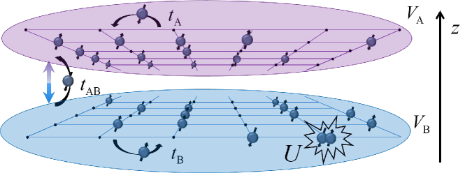
Figure 1: Schematic illustration of the bilayer-Hubbard system subjected to a perpendicular electric field. Experimentally, the bilayer system is realized by a bichromatic superlattice in the $z$ direction trapping atoms in several bilayer sheets Gall et al. (2021). The intra-layer hoppings $t_{\mathrm{A}}$ and $t_{\mathrm{B}}$ between lattice sites are controlled by the depth of the optical lattices; the inter-layer tunnelling $t_{\mathrm{AB}}$, on the other hand, is independently induced by microwaves Meng et al. (2021). Using tomographic imaging, (spin-) densities in a single layer are detected.

We consider a two-layer Hubbard model system, described by the Hamiltonian

$$H=H_{\mathrm{A}}+H_{\mathrm{B}}+H_{\mathrm{AB}},$$ (1)

with sub-Hamiltonian on each layer

$$H_{\mathrm{A}} = t_{\mathrm{A}}\sum_{\sigma=\uparrow,\downarrow}\sum_{\left\langle i,j\right\rangle}(a_{i,\sigma}^{{\dagger}}a_{j,\sigma}+\mathrm{H.c.})+U\sum_{i=1}^{N}a_{i,\uparrow}^{{\dagger}}a_{i,\downarrow}^{{\dagger}}a_{i,\downarrow}a_{i,\uparrow}$$

$$+V_{\mathrm{A}}\sum_{i=1}^{N}\left(a_{i,\uparrow}^{{\dagger}}a_{i,\uparrow}+a_{i,\downarrow}^{{\dagger}}a_{i,\downarrow}\right),$$

$$H_{\mathrm{B}} = t_{\mathrm{B}}\sum_{\sigma=\uparrow,\downarrow}\sum_{\left\langle i,j\right\rangle}(b_{i,\sigma}^{{\dagger}}b_{j,\sigma}+\mathrm{H.c.})+U\sum_{i=1}^{N}b_{i,\uparrow}^{{\dagger}}b_{i,\downarrow}^{{\dagger}}b_{i,\downarrow}b_{i,\uparrow}$$ (2)

$$+V_{\mathrm{B}}\sum_{i=1}^{N}\left(b_{i,\uparrow}^{{\dagger}}b_{i,\uparrow}+b_{i,\downarrow}^{{\dagger}}b_{i,\downarrow}\right),$$

and inter-layer hopping term

$$H_{\mathrm{AB}}=t_{\mathrm{AB}}\sum_{\sigma=\uparrow,\downarrow}\sum_{j=1}^{L}(b_{j,\sigma}^{{\dagger}}a_{j,\sigma}+\mathrm{H.c.}),$$ (3)

where $a_{i,\sigma}$ and $b_{j,\sigma}$ are fermion operators with spin-$\frac{1}{2}$ polarization $\sigma=\uparrow,\downarrow$ in layers $A$ and $B$, respectively. The parameters $t_{\mathrm{A}}(t_{\mathrm{B}})$ and $t_{\mathrm{AB}}$ are intra- and inter-layer hopping strengths, and taken to be real in this paper. The on-site interaction $U$ tends to localize the fermions by establishing a Mott insulator at half band filling. Here $H_{\mathrm{A}}$ and $H_{\mathrm{B}}$ are identical, describing a standard Hubbard model, which is restricted as simple bipartite lattice with no restriction on their geometries. In particular, the key features of the setup are: (i) $H_{\mathrm{AB}}$ is the rung of the whole system representing the tunneling between two subsystems $H_{\mathrm{A}}$ and $H_{\mathrm{B}}$. (ii) The on-site potentials $V_{\mathrm{A}}$ and $V_{\mathrm{B}}$. The gradient of such two uniform potentials acts as the electric field that can bring the migration of particles. Such two ingredients play a pivotal role in the subsequent quench dynamics. The schematic of the system is presented in Fig. 1. Driven by the advances of high-resolution microscopy, such a bilayer Fermi–Hubbard model can be realized experimentally by using ultracold atoms in an optical lattice. In particular, the bichromatic optical superlattice in the vertical direction can be employed to control the bilayer systems and inter-layer tunneling $t_{\mathrm{AB}}$ Koepsell et al. (2020); Hartke et al. (2020); Gall et al. (2021). The other Hamiltonian parameters $t_{\mathrm{A}}$, $t_{\mathrm{B}}$, $V_{\mathrm{A}}$, $V_{\mathrm{B}}$, $U$, the geometry Soltan-Panahi et al. (2011); Wirth et al. (2011); Tarruell et al. (2012); Jo et al. (2012); Shintaro et al. (2015), and the dimensionality are experimentally tunable, thus providing access to a large parameter range.

The Hamiltonian in Eq. (1) has a rich structure due to the symmetry it possesses. To gain further insight into this model, we define pseudo-spin operators

$$s^{+} = \left(s^{-}\right)^{{\dagger}}=\sum_{i=1}^{N}\left(a_{i,\uparrow}^{{\dagger}}a_{i,\downarrow}+b_{i,\uparrow}^{{\dagger}}b_{i,\downarrow}\right),$$ (4)

$$s^{z} = \frac{1}{2}\sum_{i=1}^{N}\left(a_{i,\uparrow}^{{\dagger}}a_{i,\uparrow}+b_{i,\uparrow}^{{\dagger}}b_{i,\uparrow}-a_{i,\downarrow}^{{\dagger}}a_{i,\downarrow}-b_{i,\downarrow}^{{\dagger}}b_{i,\downarrow}\right),$$ (5)

which satisfy the Lie algebra commutation relations $\left[s^{\mu},s^{\nu}\right]=\sum_{\lambda=x,y,z}2i\epsilon^{\mu\nu\lambda}s^{\lambda}$, and are employed to characterize the symmetry of the system. It can be shown that the Hamiltonian has SU(2) symmetry, obeying

$$\left[H,s^{z}\right]=\left[H,s^{\pm}\right]=0.$$ (6)

It has been shown that the ground state of $H$ with zero field at half-filling is singlet with $s=0$ Lieb (1989), or anti-ferromagnetic insulating state. The presence of the on-site potentials $V_{\mathrm{A}}$ and $V_{\mathrm{B}}$ does not break the SU(2) symmetry. It has two implications: (i) The appearance of the potential brings the possibility to change the property of the original system, such as improving the mobility of particle. (ii) The retained spin symmetry maintains the invariant subspaces, which allows us to investigate the problem in each sector. And every sector can be selected by adding an electric field in the experiment.

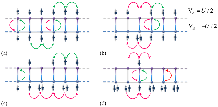
Figure 2: Sketch of the possible movement of the particles driven by a resonant electric field in a ladder system. Here we present several typical configurations to show the underlying mechanism of the transition. (a) The system is initialized in a single-occupied state such that the cooperation between the resonant electric field $V_{\mathrm{A}}=-V_{\mathrm{B}}=U/2$ and interaction $U$ only allows the migration of the particles from the $\mathrm{A}$ layer to the $\mathrm{B}$ layer. As a consequence, a hole is left in the $\mathrm{A}$ layer while a doublon is formed in the $\mathrm{B}$ layer. But the hopping of particles within each layer is strictly prohibited. (b)-(d) denote the multi-doublon and hole cases. With the constraint of energy conservation, the electron and hole can move in the non-ferromagnetic background. In particular, the spin-up particle can move freely in the upper layer while the spin-down particle (doublon) can effectively move as a single particle with the aid of the background spin configuration. The principle of the particle migration is that doublon cannot appear in the $\mathrm{A}$ layer and holes cannot appear in the $\mathrm{B}$ layer. The hopping processes denoted by red arrows are allowed, while green arrows are forbidden.

Based on the aforementioned statement, we examine the response of the system to the quenched perpendicular electric field when the interaction is free for simplicity. To this end, we introduce the Fourier transformation in two sub-systems,

$$a_{j,\sigma} = \frac{1}{\sqrt{N}}\sum_{k}e^{ikj}a_{k,\sigma},$$ (7)

$$b_{j,\sigma} = \frac{1}{\sqrt{N}}\sum_{k}e^{ikj}b_{k,\sigma},$$ (8)

where the wave vector $k=2n\pi/N$, $\left(n\in\left[-L/2,\text{ }L/2-1\right]\right)$. This transformation block diagonalizes the Hamiltonian due to its translational symmetry, i.e.,

$$H=\sum_{k,\sigma}H_{k,\sigma}=\sum_{k,\sigma}\psi_{k,\sigma}^{\dagger}h_{k,\sigma}\psi_{k,\sigma},$$ (9)

satisfying $\left[H_{k,\sigma},\text{ }H_{k^{\prime},\sigma^{\prime}}\right]=0$. Here $H$ is rewritten in the Nambu representation with the basis

$$\psi_{k,\sigma}=\left(\begin{array}[]{c}a_{k,\sigma}\\ b_{k,\sigma}\end{array}\right),$$ (10)

and $h_{k,\sigma}$ is a core matrix with the form

$$h_{k,\sigma}=\left(\begin{array}[]{cc}\lambda_{\mathrm{A}}&t_{\mathrm{AB}}\\ t_{\mathrm{AB}}&\lambda_{\mathrm{B}}\end{array}\right),$$ (11)

where $\lambda_{\mathrm{\sigma}}=-2t_{\parallel}\cos k+V_{\mathrm{\sigma}}$ ($\mathrm{\sigma=A,}$ $\mathrm{B}$). Note that $t_{\mathrm{A}}=t_{\mathrm{B}}=t_{\parallel}$ is assumed for simplicity. The Hamiltonian can be diagonalized by taking the linear transformation on $h_{k,\sigma}$. Straightforward algebra shows that

$$H=\sum_{k,\sigma}\left(\zeta_{k}+\varepsilon\right)\alpha_{k,\sigma}^{\dagger}\alpha_{k,\sigma}+\left(\zeta_{k}-\varepsilon\right)\beta_{k,\sigma}^{\dagger}\beta_{k,\sigma},$$ (12)

where

$$\zeta_{k} = -2t_{\parallel}\cos k+\frac{V_{\mathrm{A}}+V_{\mathrm{B}}}{2},$$ (13)

$$\varepsilon = \sqrt{t_{\mathrm{AB}}^{2}+\left(\frac{V_{\mathrm{A}}-V_{\mathrm{B}}}{2}\right)^{2}},$$ (14)

and

$$\alpha_{k,\sigma}^{\dagger} = \cos\frac{\theta}{2}a_{k,\sigma}^{\dagger}+\sin\frac{\theta}{2}b_{k,\sigma}^{\dagger},$$ (15)

$$\beta_{k,\sigma}^{\dagger} = \sin\frac{\theta}{2}a_{k,\sigma}^{\dagger}-\cos\frac{\theta}{2}b_{k,\sigma}^{\dagger},$$ (16)

with $\cos\theta=\left(V_{\mathrm{A}}-V_{\mathrm{B}}\right)/2\varepsilon$. Evidently, the role of the tilted potential and tunneling $t_{\mathrm{AB}}$ is to separate two identical single-particle energy bands. Hence, the ground state of the system is the direct product of spin-singlets and triplets belonging to the different $k$ subspace, given that the influence of the electric field is not considered and the system is at half-filling. The corresponding ratio between such two components is determined by $t_{\mathrm{AB}}$. In particular, the ground state is a band insulator of spin-singlets along the bonds between the layers when $t_{\mathrm{AB}}/t_{\parallel}>2$. Without loss of generality, we take the ground state of $H$ with $V_{\mathrm{A}}=V_{\mathrm{B}}=0$ at half-filling as the initial state

$$\left|\psi\left(0\right)\right\rangle=\prod_{\left|k^{\prime}\right|<k_{c}^{\prime},\sigma}a_{k^{\prime},\sigma}^{\dagger}b_{k^{\prime},\sigma}^{\dagger}\prod_{k_{c}^{\prime}<\left|k\right|<k_{c},\sigma}\frac{a_{k,\sigma}^{\dagger}-b_{k,\sigma}^{\dagger}}{\sqrt{2}}\left|\mathrm{Vac}\right\rangle,$$ (17)

where $\left|\mathrm{Vac}\right\rangle$ is the vacuum state of fermion. Here $k_{c}^{\prime}=$min$\{$arccos$(t_{\mathrm{AB}}/2t_{\parallel})$, arccos$(-t_{\mathrm{AB}}/2t_{\parallel})\}$, and $k_{c}=\pi-k_{c}^{\prime}$. After a quench, the on-site potentials $V_{\mathrm{A}}$ and $V_{\mathrm{B}}$ are applied, then the evolve state driven by $H$ can be given as

$$\left|\psi\left(t\right)\right\rangle = \prod_{\left|k^{\prime}\right|<k_{c}^{\prime},\sigma}e^{-2i\zeta_{k^{\prime}}t}a_{k^{\prime},\sigma}^{\dagger}b_{k^{\prime},\sigma}^{\dagger}\times$$ (18)

$$\prod_{k_{c}^{\prime}<\left|k\right|<k_{c},\sigma}e^{-i\zeta_{k}t}\frac{P_{-}a_{k,\sigma}^{\dagger}-P_{+}b_{k,\sigma}^{\dagger}}{\sqrt{2}}\left|\mathrm{Vac}\right\rangle,$$

where $P_{\pm}=\cos\varepsilon t+i\sin\varepsilon t\left(\sin\theta\pm\cos\theta\right)$. To measure the migration of particles, the ratio of the particle density between two layers

$$r(t)=\frac{\langle\sum_{\sigma,i=1}^{N}a_{i,\sigma}^{{\dagger}}a_{i,\sigma}\rangle}{\langle\sum_{\sigma,i=1}^{N}b_{i,\sigma}^{{\dagger}}b_{i,\sigma}\rangle},$$ (19)

is introduced. For the evolved state $\left|\psi\left(t\right)\right\rangle$, its transfer rate can be given as

$$r(t)=\frac{\sum_{\left|k^{\prime}\right|<k_{c}^{\prime},\sigma}1+\frac{1}{2}\sum_{k_{c}^{\prime}<\left|k\right|<k_{c},\sigma}\left[1-\sin 2\theta\sin^{2}\varepsilon t\right]}{\sum_{\left|k^{\prime}\right|<k_{c}^{\prime},\sigma}1+\frac{1}{2}\sum_{k_{c}^{\prime}<\left|k\right|<k_{c},\sigma}\left[1+\sin 2\theta\sin^{2}\varepsilon t\right]}.$$ (20)

Evidently, $r(t)$ exhibits a periodical behavior with period $\tau=\pi/\varepsilon$. Further, the averaged transfer ratio over a long time interval $T$ is defined as

$$\overline{r}=\lim_{T\rightarrow\infty}\frac{1}{T}\int_{0}^{T}r(t)\mathrm{d}t.$$ (21)

Direct derivation shows that

$$\overline{r}=\frac{\sum_{\left|k^{\prime}\right|<k_{c}^{\prime},\sigma}1+\frac{1}{2}\sum_{k_{c}^{\prime}<\left|k\right|<k_{c},\sigma}\left[1-\sin\theta\cos\theta\right]}{\sum_{\left|k^{\prime}\right|<k_{c}^{\prime},\sigma}1+\frac{1}{2}\sum_{k_{c}^{\prime}<\left|k\right|<k_{c},\sigma}\left[1+\sin\theta\cos\theta\right]}.$$ (22)

It indicates that the cooperation of the perpendicular field and $t_{\mathrm{AB}}$ leads to the transfer of particles between the different layers, which serves as the building block to realize the conducting phase from a Mott insulator as $U$ switches on. Note, in passing, that the direction of particle transfer depends on the choice of the initial state and is not necessarily related to the direction of gradient of the chemical potential. An obvious example is the sign reversal of $\theta$ in Eq. (22) for the highest excited state, where particles tend to go from layer $\mathrm{B}$ to layer A. It is in stark difference from the classical system in which the flow of particles is along the direction of the gradient of the potential. On the other hand, in the absence of $U$, the transfer rate between two layers oscillates such that the system acquires the information of the initial state once the time $t=n\tau$ ($n$ is a positive integer). In other words, the presence of potential only induces the particle migration and does not result in the imbalance of particle density between two layers over a long time interval.

In the following, we study the dynamical response of the ground state of $H$ (large $U$) to a quenched electric field with the resonant value.

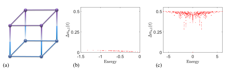
Figure 3: Plots of the local charge fluctuation $\Delta n_{a,1}$ for the low energy excitation of the Hubbard model at half-filling. The geometry of the considered two-layer system is illustrated in Fig. 3(a). The other system parameters are given as (b) $t_{\mathrm{B}}/t_{\mathrm{A}}=1$, $V=0$, and $U/t_{\mathrm{A}}=20$ (c) $t_{\mathrm{B}}/t_{\mathrm{A}}=1$, $V/t_{\mathrm{A}}=5$, and $U/t_{\mathrm{A}}=20$. In Fig. 3(b), the system favors the Mott-insulating phase and hence $\Delta n_{a,1}$ of low-energy eigenstates are around $0$. However, $\Delta n_{a,1}$ is around $0.5$ except for very few eigenstates when the resonant field $V$ presents. The cooperation between $U$ and $V$ results in a dramatic change in the system conductivity.

III Resonant field

Meanfiled theory Sachdev (2011) has shown that the phase diagram of a Hubbard model is described by the Mott lobe, which is a function of $U$ and chemical potential. The formation of the anti-ferromagnetic insulating ground state requires large $U$ and half-filling. For the bilayer system, we note that the total particle number of the two-layer is conservative, while the one of each layer is not. In this work we consider the case with fixed particle number, which equals to $2N$. Thus when taking $V_{\mathrm{A}}=V_{\mathrm{B}}$, the ground state is an anti-ferromagnetic insulating state. However, when taking $V_{\mathrm{A}}\neq V_{\mathrm{B}}$, the chemical potentials can adjust the particle density on each layer, since one layer can act as a source of particles for the other. It happens by the difference of the chemical potential, or the perpendicular electric field. In the following, we will show that an optimal field can provide a resonant channel for the directional migration of particles from one layer to the other.

We start with the simplest case with $t_{\mathrm{A}}=t_{\mathrm{B}}=t_{\mathrm{AB}}=V_{\mathrm{A}}=V_{\mathrm{B}}=0$. The Hamiltonian only contains the repulsive term, i.e., $U\sum_{i=1}^{N}\left(a_{i,\uparrow}^{{\dagger}}a_{i,\downarrow}^{{\dagger}}a_{i,\downarrow}a_{i,\uparrow}+b_{i,\uparrow}^{{\dagger}}b_{i,\downarrow}^{{\dagger}}b_{i,\downarrow}b_{i,\uparrow}\right)$, and then the ground states in the subspace with zero $s^{z}$ are multi-degenerate. The energy is zero and the degenerate degree is $\mathcal{N}_{\mathrm{I}}=C_{2N}^{N}$, the explicit expression of which is $C_{2N}^{N}=(2N)!/[(2N-N)!(N)!]$. These states construct singlet ground state when parameters $t_{\mathrm{A}}=t_{\mathrm{B}}=t_{\mathrm{AB}}$ are switched on in large $U$ limit, and are referred to as the insulating set (I-set) of states in this paper.

Now we consider the case with $t_{\mathrm{A}}=t_{\mathrm{B}}=t_{\mathrm{AB}}$, and $V_{\mathrm{A}}=-V_{\mathrm{B}}=U/2$ (hereafter $V_{\mathrm{A}}=-V_{\mathrm{B}}=V$), which is referred to as the resonant field. The Hamiltonian can be rewritten in the from

$$H_{\mathrm{A}} = U/2\sum_{i=1}^{N}\left(a_{i,\uparrow}^{{\dagger}}a_{i,\uparrow}+a_{i,\downarrow}^{{\dagger}}a_{i,\downarrow}\right)^{2},$$ (23)

$$H_{\mathrm{B}} = -U/2\sum_{i=1}^{N}\left(b_{i,\uparrow}^{{\dagger}}b_{i,\uparrow}-b_{i,\downarrow}^{{\dagger}}b_{i,\downarrow}\right)^{2},$$ (24)

which is convenient for the following analysis. The eigen energy of $H_{\mathrm{A}}+H_{\mathrm{B}}$ is

$$E=U/2\sum_{i=1}^{N}\left[\left(n_{\mathrm{A,}i,\uparrow}+n_{\mathrm{A,}i,\downarrow}\right)^{2}-\left(n_{\mathrm{B,}i,\uparrow}-n_{\mathrm{B,}i,\downarrow}\right)^{2}\right],$$ (25)

where $n_{a\mathrm{,}i,\sigma}$ and $n_{b\mathrm{,}i,\sigma}$ are eigen values of operators $a_{i,\sigma}^{{\dagger}}a_{i,\sigma}$ and $b_{i,\sigma}^{{\dagger}}b_{i,\sigma}$, respectively. For the half-filled case in the subspace with zero spin component in $z$ direction, we have the following constraint conditions

$$\sum_{\sigma=\uparrow,\downarrow}\left(N_{a\mathrm{,}\sigma}+N_{b\mathrm{,}\sigma}\right) = 2N,$$ (26)

$$N_{a\mathrm{,}\uparrow}+N_{b\mathrm{,}\uparrow}-N_{a\mathrm{,}\downarrow}-N_{b\mathrm{,}\downarrow} = 0,$$ (27)

where $N_{a\mathrm{,}\sigma}$ and $N_{b\mathrm{,}\sigma}$ denote the eigen values of operators $\sum_{i=1}^{N}a_{i,\sigma}^{{\dagger}}a_{i,\sigma}$ and $\sum_{i=1}^{N}b_{i,\sigma}^{{\dagger}}b_{i,\sigma}$, respectively. Notice that when every site is occupied by a single particle, we have $\left(n_{a\mathrm{,}i,\uparrow}+n_{a\mathrm{,}i,\downarrow}\right)^{2}=\left(n_{b\mathrm{,}i,\uparrow}-n_{b\mathrm{,}i,\downarrow}\right)^{2}=1$ for all $i\in\left[1,N\right]$ such that the ground state energy is $E=0$. In the following, we analyse all the possible eigenstates with zero energy, since the number and configuration of which are important for our results. As the mentioned above, the number of single-occupied states is $\mathcal{N}_{\mathrm{I}}$ and the superposition of these states constructs the anti-ferromagnetic groundstate of the original Hamiltonian with large $U$ and zero $V$. Based on such states, losing a particle in layer $\mathrm{A}$ results in energy lose of $U/2$, while gaining a fermion in layer B results in energy lose of $-U/2$, generating a new zero energy state. Accordingly, a set of zero energy states can be constructed by losing $n$ ($n\in\left[1,N\right]$) particles in layer $\mathrm{A}$ and gaining $n$ particle in layer B. The number of such kind of states is $\left(C_{N}^{n}\right)^{2}C_{2N-2n}^{N-n}$, in which term $C_{N}^{n}$ comes from the configuration of hole in layer $\mathrm{A}$ or the doublon in layer B, and $C_{2N-2n}^{N-n}$ comes from the spin configuration of the rest single-occupied particles. Then the total number of zero-energy (ground) states is $\mathcal{N}_{\mathrm{C}}=\sum_{j=1}^{N}(C_{N}^{j})^{2}C_{2N-2j}^{N-j}$. All these states are hybridized by the inter-chain and intra-chain hoppings. In other words, the hopping terms can drive one of these states to all the rest states.

IV the mobility of the free doublons and holes

In this section, we discuss the observable results based on the analysis in the last section. We can classify all states into two sets: (i) I-set (insulating set), as mentioned above, which consists of complete single-occupied states; (ii) C-set (conducting set), which consists of states involving holes and doublons. The reason for such a classification is that the superposition of states in I-set describes an antiferromagnetic Mott insulating state, while the superposition of states in C-set describes a conducting state. We explain the reason for the classification via the following examples. For simplicity, we consider the simplest case involving states with single-hole and single-doublon. A set representative of states in C-set can be expressed as the form $a_{i,\uparrow}b_{i,\uparrow}^{{\dagger}}\left|\Uparrow\right\rangle_{\mathrm{A}}\left|\Downarrow\right\rangle_{\mathrm{B}}$, where states $\left|\Uparrow\right\rangle_{\mathrm{A}}=\prod_{l=1}^{N}a_{l,\uparrow}^{{\dagger}}\left|\mathrm{Vac}\right\rangle$ and $\left|\Downarrow\right\rangle_{\mathrm{B}}=\prod_{l=1}^{N}b_{l,\downarrow}^{{\dagger}}\left|\mathrm{Vac}\right\rangle$ denote ferromagnetic states of A and B layers, respectively, and $\left|\mathrm{Vac}\right\rangle$ is the empty state of the whole system. Obviously, the dynamics of hole and electron on each layers can act as free carriers on the ferromagnetic background. Likewise, similar situation occurs for multi-hole and doublon cases, and for other types of non-ferromagnetic background. For clarity, we sketch some typical cases in Fig. 2.

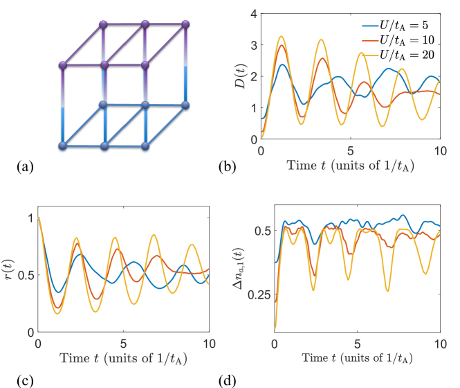
Figure 4: Numerical simulation of the quenched bilayer Hubbard system for different repulsive interactions $U/t_{\mathrm{A}}=5$, $10$, and $20$. The system consists of two coupled ladders and is initialized in the ground state of $H_{\mathrm{pre}}$. The small charge fluctuation of the initial ground state arises from the finite interaction which allows the existence of a double-occupied state with $s=0$. Such non-ferromagnetic kind of states is suppressed when $U$ increases. After a quench, the doublons and holes appear in the evolved state due to the particle flow from the upper layer to the lower layer as shown in Fig. 3(a). This is protected by the energy shell residing in the low-energy excited subspace. In the non-ferromagnetic background, the non-equilibrium system enters into the conducting phase manifested by the increase of the charge fluctuation. Note that the layers A and B share the same charge fluctuation $\Delta n_{a,j}=\Delta n_{b,j}=\Delta n_{j}$ since both free electrons and holes play the same role in the particle migration.

In order to predict the dynamical behavior of the quench, we estimate the following two quantities. The first one is the ratio of the dimensions of insulating and conducting classes. Straightforward calculation gives

$$r_{1}=\frac{\mathcal{N}_{\mathrm{I}}}{\mathcal{N}_{\mathrm{C}}}\approx e^{-\gamma N},$$ (28)

where factor $\gamma=0.325$ is obtained from the numerical fitting. The second one is the ratio of the average particle numbers between insulating and conducting classes. Considering a mixed state, in which all the zero-energy states have the same probability, we have the average numbers on each layers

$$\overline{N}_{\mathrm{A,}\uparrow} = \overline{N}_{\mathrm{A,}\downarrow}=\frac{\sum_{j=1}^{N}j(C_{N}^{j})^{2}C_{2N-2j}^{N-j}}{\mathcal{N}_{\mathrm{I}}+\mathcal{N}_{\mathrm{C}}}=\frac{N}{3},$$ (29)

$$\overline{N}_{\mathrm{B,}\uparrow} = \overline{N}_{\mathrm{B,}\downarrow}=\frac{\sum_{j=1}^{N}j(C_{N}^{j})^{2}C_{2j}^{j}}{\mathcal{N}_{\mathrm{I}}+\mathcal{N}_{\mathrm{C}}}=\frac{2N}{3},$$ (30)

which result in

$$r_{2}=\frac{\overline{N}_{\mathrm{A,}\uparrow}+\overline{N}_{\mathrm{A,}\downarrow}}{\overline{N}_{\mathrm{B,}\uparrow}+\overline{N}_{\mathrm{B,}\downarrow}}=1/2.$$ (31)

These two quantities imply the following predictions. (i) The initial state has a very small portion ($r_{1}$) comparing to the possible evolved states, which will never go back to the initial one. It is similar to the case with a site initial state in a square lattice. The probability will spread out, approaching to uniform distribution after a long time. Then the evolved state probably relaxes to a conducting state. (ii) The value of $r_{2}$ indicates that the ratio of numbers on two layers turns to be $0.5$ after a long time. It predicts that there is a particle flow in the quench dynamical process.

In order to capture the main consequence of the particle flow arising from the cooperation of $U$ and resonant $V$, we further introduce the local charge fluctuation $\Delta n_{\lambda,j}$ to compare the conductivity of the eigenstates before and after quench. The definition of $\Delta n_{\lambda,j}$ is given by

$$\Delta n_{\lambda,j}=\sqrt{\Delta_{1,\lambda,j}-\Delta_{2,\lambda,j}^{2}}\quad(\lambda=a,b),$$ (32)

where

$$\Delta_{1,\lambda,j} = \langle(\sum_{\sigma}\lambda_{j,\sigma}^{{\dagger}}\lambda_{j,\sigma})^{2}\rangle,$$ (33)

$$\Delta_{2,\lambda,j} = \langle\sum_{\sigma}\lambda_{j,\sigma}^{{\dagger}}\lambda_{j,\sigma}\rangle.$$ (34)

Specifically, if the system is in the Mott insulating phase, such fluctuation would become energetically unfavorable, forcing the system into a number state and exhibiting a vanishing particle number fluctuation $\Delta n_{\lambda,j}$. Beyond the Mott insulator regime, the fermions are delocalized with the non-vanishing charge fluctuation. In Fig. 3, we figure out the conductivity of the eigenstates in the cases of $H\left(V=0\right)$ and $H\left(V=U/2\right)$, respectively. The system is at symmetric half filling, i.e., $s^{z}=0$, and its geometry is illustrated in Fig. 3(a). We focus on the low-lying eigenstates whose energy is around $0$. When $V=0$ and large $U$ limit, the low energy excitation of the considered half-filled Hubbard model can be effectively described by the Heisenberg model with two layers. The corresponding eigenstates are the superposition of bases belonging to the I-set. As such, the charge fluctuation $\Delta n_{a,1}$ is about $0$ as shown in Fig. 3(b). Conversely, the low-lying eigenstates of $H\left(V=U/2\right)$ possess the non-zero charge fluctuation since C-set dominates especially in the large $N$ limit. This can be seen in Fig. 3(c). The local charge fluctuation for most eigenstates is $0.5$. To gain further insight into the dynamics of the two-layer system, we consider an initial state expanded in such energy shell,

$$\left|\psi\left(0\right)\right\rangle=\sum_{\alpha}c_{\alpha}\left|E_{\alpha}\right\rangle\text{,}$$ (35)

where $\left|E_{\alpha}\right\rangle$ is the eigenstate of $H$ with eigenvalue $E_{\alpha}$ in the low-lying energy shell. The expectation value of a local operator $\widehat{O}$ as a function of time thus reads

$$O\left(t\right) \equiv \left\langle\psi\left(t\right)\right|\widehat{O}\left|\psi\left(t\right)\right\rangle$$ (36)

$$= \sum_{\alpha}\left|c_{\alpha}\right|^{2}O_{\alpha\alpha}+\sum_{\alpha\neq\beta}O_{\alpha\beta}e^{i\left(E_{\alpha}-E_{\beta}\right)t},$$

where $O_{\alpha\alpha}=\left\langle E_{\alpha}\right|\widehat{O}\left|E_{\alpha}\right\rangle$ and $\widehat{O}$ stands for either the operator $(\sum_{\sigma}\lambda_{j,\sigma}^{{\dagger}}\lambda_{j,\sigma})^{2}$ or $\sum_{\sigma}\lambda_{j,\sigma}^{{\dagger}}\lambda_{j,\sigma}$ in the considered two-layer system. Due to phase cancellation of the off-diagonal terms in Eq. (36), the long-time average is determined only by the average in the diagonal element such that

$$\overline{O}\left(t\right)=\lim_{T\rightarrow\infty}\frac{1}{T}\int_{0}^{T}O\left(t\right)\mathrm{d}t=\sum_{\alpha}\left|c_{\alpha}\right|^{2}O_{\alpha\alpha}.$$ (37)

For the considered two types of the systems $H\left(V=0\right)$ and $H\left(V=U/2\right)$, $O_{\alpha\alpha}$ approaches a constant number for the most eigenstates of the low-lying energy sector. Hence, $\overline{O}\left(t\right)=O_{\alpha\alpha}$ indicating that the eigenstate and arbitrary evolved state share the same average value of $\Delta n_{\lambda,j}$. It can be expected that the initial state containing the insulating component will tend to the conducting state after a long-time evolution. In the subsequent section, we will demonstrate this point through a quench process.

Before ending this section, we want to point out that the conducting mechanism is different from that of the single-layer system wherein the particles are not half-filling. For the latter system, the maximum of holes is contingent on the filled particle number. As for the two-layer system, layer A acts as a source of particles for layer B, and the corresponding particle number of layer A is not conserved. As a consequence, layer A involves all the possible configurations of holes in the low-energy sector, which provides more channels for the transfer of particles between the layers. The cooperation between $U$ and the resonant $V$ can stabilize the system in this phase for a long time.

V Dynamical density transfer

The above analysis provides a prediction about the dynamical transition from an insulating state to a conducting state in a composite system. In a slightly different language, the main point of the above consideration can be viewed as follows. A Mott insulating state is essentially the result of Pauli exclusion principle and Coulomb repulsion at half-filling. It is not a stable equilibrium since the chemical potential can change the particle density for an open system. For a half-filled bilayer Hubbard system with zero fields, the ground state lies at the equilibrium point for each layer. When the resonant external field is switched on, the low-energy eigenstates changes dramatically with positive or negative doping in each layer. This exactly compensates for repulsive interactions presents in the Hubbard model such that the transfer of particles between the two layers cost free. As a consequence, many nearly degenerate conducting states lie at the low-energy sector of quenched Hamiltonian which allows an easier transfer of particles between layers.

We perform numerical simulations on a finite system for the following quench process. The pre-quench Hamiltonian is assumed as $H_{\mathrm{pre}}=H$ with $t_{\mathrm{A}}=t_{\mathrm{B}}=t_{\mathrm{AB}}=1$, and $V=0$. The post-quench Hamiltonian is then $H_{\mathrm{pos}}=H$ with $V=U/2$. Initially, the system is half-filled and at the ground state, being an insulating state with a strong anti-ferromagnetic correlation. According to our analysis, the quench dynamics should result in a steady conducting state, realizing the dynamical transition from an insulating state to a conducting state. The evolved states $\left|\Psi\left(t\right)\right\rangle$ for initial anti-ferromagnetic ground state $\left|\Psi\left(0\right)\right\rangle$ is calculated by exact diagonalization method. We focus on the following quantities: (i) The ratio of particle density between two layers $r(t)$ which is a key signature of the dynamical transition; (ii) The number fluctuation $\Delta n_{\lambda,j}$ of the evolved state $\left|\Psi\left(t\right)\right\rangle$.

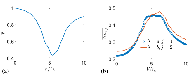
Figure 5: Average $\overline{r}$ and $\overline{\Delta n_{\lambda,j}}$ as functions of $V$ for $12$-site Hubbard model at half filling and $s_{z}=0$. The initial state is prepared as the ground state of $H_{\mathrm{pre}}$. The system parameters are $U/t_{\mathrm{A}}=10$ and cutoff quench time $T=50/t_{\mathrm{A}}$. It indicates that, as $V$ approaches $U/2$, a dip will appear verifying our prediction in the text.

The lattice geometry and numerical results are plotted in Fig. 4, where a $12$-site Hubbard model at half filling is considered. It can be shown that the resonant electric field can induce the particle transfer from the upper layer to the lower layer forming the doublons and holes in the evolved state. This can be demonstrated by the increase of total double occupancy $D=\sum_{j}\langle D_{j}\rangle$, where the local double-occupation operator is given by $D_{\lambda,j}=\lambda_{j,\uparrow}^{\dagger}\lambda_{j,\uparrow}\lambda_{j,\downarrow}^{\dagger}\lambda_{j,\downarrow}$ ($\lambda=a,$ $b$). The movable electrons and holes significantly increase the number fluctuations of both layers and hence enhances the conductivity. Such a mechanism still holds even in the small $U$ condition which can be shown by comparing Figs. 4 (b)-(d). The weak interaction means that the ground state does not fully consist of the single-occupied Mott insulating state such that the initial double occupancy and charge fluctuation is not zero, which can be shown in Figs. 4 (b) and (d). Instead, the portion of the other state $s=0$, i.e., doublon state, increases leading to the non-zero number fluctuation of the initial state and total transfer rate between the two layers. It indicates that the effectiveness of the scheme is suppressed due to the tunneling between the considered energy shell (I- and C-set) and other energy levels. To further check the validity of the earlier analysis, we introduce the average number fluctuation

$$\overline{\Delta n}_{\lambda,j}=\lim_{T\rightarrow\infty}\frac{1}{T}\int_{0}^{T}\Delta n_{\lambda,j}\mathrm{d}t,$$ (38)

to compare the results of the resonant and non-resonant cases. Average $\overline{r}$ and $\overline{\Delta n}_{\lambda,j}$ as functions of parameter $V$ for different $j$ are plotted in Fig. 5. It can be shown that the dips appear in both $\overline{r}$ and $\overline{\Delta n}_{\lambda,j}$ when the resonant electric field is taken. Another interesting phenomenon is that both layers share the same conducting behavior manifested by the performance of $\overline{\Delta n}_{a,j}$ and $\overline{\Delta n}_{b,j}$. This can be understood as follow: Assume that the initial state is prepared as the direct product of ferromagnetic states within each layer, i.e., $\left|\Uparrow\right\rangle_{\mathrm{A}}\left|\Downarrow\right\rangle_{\mathrm{B}}$. The resonant electric field makes the spin-up particle migrates from the layer $\mathrm{A}$ to $\mathrm{B}$ such that a hole and a doublon are formed in two layers individually. The spin-up particle can move freely based on the spin-down ferromagnetic background while the formation of the hole enable the hopping of the spin-down particles. Although the free particles are formed in different ways in two layers, both facilitate the movement of particles within each layer and thus increase the conductivity. Note that such a steady state is the consequence of the non-equilibrium many-body dynamics that is usually absent in the ground-state phase. Before ending this part, it is worthy pointing out that the lattice structure of real materials, such as bilayer graphene, is composed of coupled layers and is therefore not strictly two-dimensional. Another advantage of our scheme is that it is not only applicable to the bilayer system. Instead, it still makes sense even in the multi-layer system. The core is that the interplay between the resonant electric field and interaction can hybridize a small number of insulating states and a large number of conducting states such that the particles tend to move in each layer rather than localize at each site.

VI Summary

In summary, we have systematically investigated the quench dynamics of the bilayer Hubbard model subjected to a perpendicular electric field. In the presence of the resonance electric field, the system can enter into the steady conducting phase via a non-equilibrium scheme, which can be demonstrated by the increase of the charge fluctuation. The underlying mechanism is that the cooperation between the resonant electric field and on-site interaction $U$ provides an energy shell hybridizing the single-and double-occupied states with $s=0$. Due to the energy gap determined by the large $U$ and resonant field, the inter- and intra- layer hopping does not induce the tunneling between the considered shell and other shells so that the dynamics in the quasi subspace is protected by the so-called ”energy conservation”. The stable hybridization of such two kinds of states allow the directional particle flow between the two layers, which forms the holes in the A layer and doublon in the B layer. This facilitates the movement of the particles within each layer and hence enhances the conductivity. The particles exhibit the same conducting behavior in both layers since the formation of the free particles shares a similar mechanism in both layers. Due to the large proportion of double-occupied states in the resonant energy shell, a non-equilibrium system can accommodate such a conducting state for a long time. Our findings establish a strategy for enhancing the conductivity of the multi-layer strongly correlated system from an out of equilibrium method.