Steady off-diagonal long-range order state in a half-filled dimerized Hubbard chain induced by a resonant pulsed field

Abstract

We show that a resonant pulsed field can induce a steady superconducting state even in the deep Mott insulating phase of the dimerized Hubbard model. The superconductivity found here in the non-equilibrium steady state is due to the $\eta$-pairing mechanism, characterized by the existence of the off-diagonal long-range order (ODLRO), and is absent in the ground-state phase diagram. The key of the scheme lies in the generation of the field-induced charge density wave (CDW) state that is from the valence bond solid. The dynamics of this state resides in the highly-excited subspace of dimerized Hubbard model and is dominated by a $\eta$-spin ferromagnetic model. The decay of such long-living excitation is suppressed because of energy conservation. We also develop a dynamical method to detect the ODLRO of the non-equilibrium steady state. Our finding demonstrates that the non-equilibrium many-body dynamics induced by the interplay between the resonant external field and electron-electron interaction is an alternative pathway to access a new exotic quantum state, and also provides an alternative mechanism for enhancing superconductivity.

I Introduction

Driving is not only a transformative tool to investigate complex many-body system but also makes it possible to create non-equilibrium phase of quantum matter with desirable properties Verstraete et al. (2009); Ichikawa et al. (2011); Eisert et al. (2015); Basov et al. (2017); Mor et al. (2017); Cavalleri (2018); Ishihara (2019). It can significantly alter the microscopic behavior of strongly correlated system and manifest a variety of collective and cooperative phenomena at the macroscopic level. Spurred on by experiments in ultra-cold atomic gases, the non-equilibrium strongly correlated systems have been the subject of intense study over the last decade Greiner et al. (2002); Freericks et al. (2006); Bloch et al. (2008); Freericks (2008); Aron et al. (2012); Aoki et al. (2014); Essler and Fagotti (2016); Vidmar and Rigol (2016); Vasseur and Moore (2016); Wang et al. (2016); Zhang and Song (2020); Rubio-Abadal et al. (2020); Moudgalya et al. (2020); Wei et al. (2021); Zhang and Song (2022). Additionally, pump-probe spectroscopy offers a new avenue for the exploration of available electronic states in correlated materials Perfetti et al. (2006). Among them, the most striking is the discovery of photoinduced transient superconducting behaviors in some high-$T_{c}$ cuprates Fausti et al. (2011); Hu et al. (2014); Kaiser et al. (2014) and alkali-doped fullerenes Mitrano et al. (2016); Cantaluppi et al. (2018). All these advances have revived interest in the fundamental behavior of quantum systems away from equilibrium.

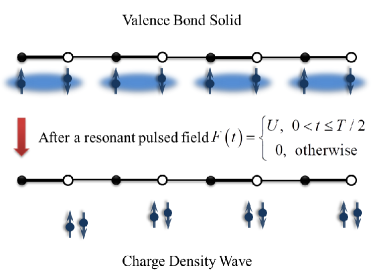
Figure 1: Schematic illustration of the dynamical pairing process considered in this work. The system is initialized in a dimerized Hubbard model at half filling. The strong dimerization divides the whole $2N$ lattice into $N$ unitcells. In each unitcell, two electron spins form a spin $0$ singlet due to the antiferromagnetic interaction, while not being entangled with the spins of other unitcell. Hence, the gound state is a valence bond solid. The resonant pulsed field $F$ plays the role in each unitcell individually such that the CDW state can be generated after a period $T/2$ with $T=\pi/\Delta$. Then the CDW state will evolve to an ODLRO state via doublon diffusion, which is the key to realizing the non-equilibrium superconducting phase.

Non-equilibrium control of quantum matter is an intriguing prospect with potentially important technological applications Yonemitsu and Nasu (2008); Giannetti et al. (2016); Oka and Kitamura (2019); de la Torre et al. (2021). Experiments with various materials and excitation conditions have witnessed phenomena with no equilibrium analog or accessibility of chemical substitution, including superconducting-like phases Fausti et al. (2011); Mitrano et al. (2016); Cavalleri (2018); Suzuki et al. (2019), charge density waves (CDW) Stojchevska et al. (2014); Matsuzaki et al. (2014); Kogar et al. (2020) and excitonic condensation Murotani et al. (2019). Among various non-equilibrium protocols, the generation of the $\eta$-pairing-like state possessing the off-diagonal long-range order (ODLRO), originally proposed by Yang for the Hubbard model Yang (1989), plays a pivotal role in which the existence of doublon and holes facilitate the superconductivity Kitamura and Aoki (2016); Kaneko et al. (2019); Tindall et al. (2019); Fujiuchi et al. (2019); Peronaci et al. (2020); Fujiuchi et al. (2020); Ejima et al. (2020); Li et al. (2020); Kaneko et al. (2020); Zhang and Song (2021). Therefore, how to stabilize a system in a non-equilibrium superconducting phase with a long lifetime is a great challenge and is at the forefront of current research. Besides, constructing a clear and simple physical picture to realize the non-equilibrium superconducting phase for the experiment is also the goal of on-going theoretical investigation.

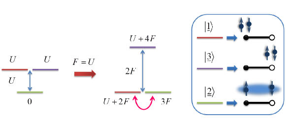
Figure 2: Sketch of the resonant pairing mechanism in the two-site Hubbard model at half-filling. The system can be divided into two subspaces labeled by the spin quantum numbers $s=0$, and $s=1$. We focus on the subspace with $s=0$. The double-occupied bases are denoted by red and purple lines and the green line indicates the valence bond state that is the GS when $U/\kappa\gg 1$. In the absence of $F$, there exists an energy difference of $U$ between such two types of states. The resonant $F$ places the valence bond state and red double-occupied state on the same energy shell such that the kinetic term allows a transfer between these two states. The gap $2F$ prohibits the tunneling from the lower two states to the upper purple state and hence protects the formation of the CDW state in the whole lattice.

It is the aim of this paper to unveil the underlying mechanism of superconductivity in a non-equilibrium matter. The core is how to excite a Mott insulator to a pairing state (CDW state) within the highly excited subspace. Then it evolves to a steady ODLRO state. To this end, we consider a repulsive dimerized Hubbard model, in which the dimerization can control the type of the ground state but does not change the magnetic correlation. The strong dimerization can make the main component of the anti-ferromagnetic ground state change from a Neel state to a valence bond solid where the electrons belonging to the different unitcells are not entangled with each other. This allows that the resonant pulsed field can drive the spin singlet state to a double-occupied state in each unitcell so that the CDW state is constructed in the entire lattice. The doublons and holes can significantly enhance the conductivity of the system. Fig. 1 illustrates this core dynamics of the proposed non-equilibrium scheme. Note that non-resonant external field will also increase the conductivity of the system, but will not form a CDW state with maximized doublons and holes. This does not favor the superconductivity in the subsequent dynamics. Due to the energy conservation, the system can stay in the highly-excited subspace, which shares the same energy shell with the CDW state, for a long time. The corresponding doublon dynamics can be fully captured by the effective $\eta$-spin ferromagnetic model that can be obtained through the virtual exchange of the particles. In this context, such an effective Hamiltonian can drive the CDW state to a steady state which distributes evenly in the lattice and possess the long-range $\eta$-spin correlation. This is the characteristic of the system entering the non-equilibrium superconducting phase. By introducing the magnetic flux, we further develop a method of detecting this kind of non-equilibrium phase of matter based on the performance of the Loschmidt echo (LE). Specifically, the characteristic that LE shows periodical behavior rather than a constant value around $1$ can be used to detect whether the system is in the superconducting phase. It is hoped that these results can motivate further studies of both the fundamental aspects and potential applications of the non-equilibrium interacting system.

The remainder of this paper is organized as follows. In Sec. II, we first present the pairing dynamics induced by the resonant pulsed field. Second, we explore the long-time dynamics of a single doublon and extend the results to the multi-doublon case, which paves the way to achieve the effective $\eta$-spin model and hence facilitates the understanding of the steady ODLRO state. In Sec. III, we propose a dynamical scheme to excite the system into the non-equilibrium superconducting phase based on the repulsive dimerized Hubbard model. Correspondingly, a dynamical detection method is constructed to examine such a phase. Finally, we conclude our results in Sec. IV. Some details of our calculation are placed in the Appendix.

II Two simple models to elucidate the underlying mechanism

Recently, much attention has been paid to the realization of the superconductivity in the deep Mott insulator phase via out-of-equilibrium dynamics, e.g., quench dynamics. The underlying mechanism can be attributed to the $\eta$-pairing state induced by the external field. From a deep level, however, such a statement is neither complete nor the corresponding dynamic process is clear. In this section, we provide two examples to unravel the field-induced superconductivity. Such two models correspond to the two key parts of the entire dynamic process, namely the pairing induced by the external field and the formation of the long-range correlation via diffusion of doublon.

II.1 pairing induced by a resonant tilted fled

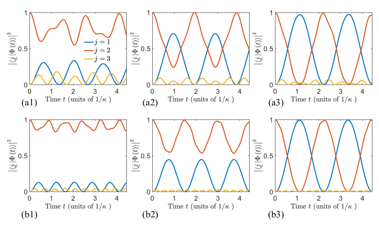
Figure 3: Dynamical pairing of the $2$-site Hubbard model at half filling for the different pulsed fields: (a1)-(b1) $F/U=0.3$; (a2)-(b2) $F/U=0.7$; (a3)-(b3) $F/U=1$; The other system parameters are (a1)-(a3) $U=5\kappa$, and (b1)-(b3) $U=10\kappa$. It can be shown that the resonant pulsed field can bring about the transition of the initial state from the valence bond state to pairing state. The corresponding transfer period is $\pi/2\Delta$, which agrees with the theoretical result in the main text. When the non-resonant external field is introduced, there will still be some double-occupancy components in the evolved state, which is beneficial to the conductivity of the system. In principle, the larger $U$, the larger the gap in the system and therefore more efficient this transition. However, we can find that, by comparing the Figs. (a) and (b), the efficiency of this dynamical scheme is still good even when a small $U$ is applied.

We start from the 1D Hubbard model subjected to a tilted field, the Hamiltonian of which is given by

$$H=H_{\mathrm{o}}+H_{\text{{e}}},$$ (1)

with

$$H_{\mathrm{o}} = -\kappa\sum_{j,\sigma}(c_{j,\sigma}^{\dagger}c_{j+1,\sigma}+\text{H.c.})+U\sum_{j}n_{j,\uparrow}n_{j,\downarrow},$$ (2)

$$H_{\text{{e}}} = F\sum_{j,\sigma}jn_{j,\sigma},$$ (3)

where $c_{i,\sigma}$ ($c_{i,\sigma}^{\dagger}$) is the annihilation (creation) operator for an electron at site $i$ with spin $\sigma\left(=\uparrow,\downarrow\right)$, and $n_{i,\sigma}=c_{i,\sigma}^{\dagger}c_{i,\sigma}$. $\kappa$ is the hopping integral between the nearest-neighboring sites, while $U>0$ is the on-site repulsive interaction. To gain further insights into the field-induced paring, we first analyze the symmetry of the system. When the titled field is switched off, the system $H_{\mathrm{o}}$ respects the spin symmetry characterized by the generators

$$s^{+} = \left(s^{-}\right)^{\dagger}=\sum_{j}s_{j}^{+},$$ (4)

$$s^{z} = \sum_{j}s_{j}^{z},$$ (5)

where the local operators $s_{j}^{+}=c_{j,\uparrow}^{\dagger}c_{j,\downarrow}$ and $s_{j}^{z}=\left(n_{j,\uparrow}-n_{j,\downarrow}\right)/2$ obey the Lie algebra, i.e., $[s_{j}^{+},$ $s_{j}^{-}]=2s_{j}^{z}$, and $[s_{j}^{z},$ $s_{j}^{\pm}]=\pm s_{j}^{\pm}$. Because of the commutation relation $[H_{\mathrm{o}}$, $\eta^{+}]=U\eta^{+}$, the system has a set of eigenstates generated by the $\eta$-pairing operators, i.e., {$\left(\eta^{+}\right)^{N_{\eta}}|\mathrm{Vac}\rangle$} where $|\mathrm{Vac}\rangle$ is a vacuum state with no electrons and $N_{\eta}$ is the number of $\eta$ pairs. Here, $\eta$ operator can be explicitly written down as

$$\eta^{+} = \left(\eta^{-}\right)^{\dagger}=\sum_{j}\eta_{j}^{+},$$ (6)

$$\eta^{z} = \sum_{j}\eta_{j}^{z},$$ (7)

with $\eta_{j}^{+}=\left(-1\right)^{j}c_{j,\uparrow}^{\dagger}c_{j,\downarrow}$ and $\eta_{j}^{z}=\left(n_{j,\uparrow}+n_{j,\downarrow}-1\right)/2$ satisfying commutation relation, i.e., $[\eta_{j}^{+},$ $\eta_{j}^{-}]=2\eta_{j}^{z}$, and $[\eta_{j}^{z},$ $\eta_{j}^{\pm}]=\pm\eta_{j}^{\pm}$. At half-filling, the ground state (GS) of $H_{\mathrm{o}}$ resides in the subspace with quantum number $s^{2}=0$, $s^{z}=0$, and is often refereed to as the anti-ferromagnetic ground state in the large $U$ limit ($U/\kappa\gg 1$). It mainly consists of the Neel state. To give further insight into the pairing mechanism, we consider a two-site system, wherein the GS becomes a single valence bond state with the form of $(c_{1,\uparrow}^{\dagger}c_{2,\downarrow}^{\dagger}-c_{1,\downarrow}^{\dagger}c_{2,\uparrow}^{\dagger})/\sqrt{2}|\mathrm{Vac}\rangle$. The presence of $H_{\text{{e}}}$ does not break the first spin symmetry but change the property of the GS. What we are interested in is how does the system response to the tilted field if the system is initialized in the GS of $H_{\mathrm{o}}$. For clarity, the matrix form of Hamiltonian (1) is written as

$$H=\left(\begin{array}[]{ccc}U+2F&-\sqrt{2}\kappa&0\\ -\sqrt{2}\kappa&3F&-\sqrt{2}\kappa\\ 0&-\sqrt{2}\kappa&U+4F\end{array}\right),$$ (8)

in the invariant subspace $s^{2}=0$, $s^{z}=0$ under the basis of {$|\underline{j}\rangle$}, where

$$|\underline{1}\rangle = c_{1,\uparrow}^{\dagger}c_{1,\downarrow}^{\dagger}|\mathrm{Vac}\rangle,$$ (9)

$$|\underline{2}\rangle = \frac{1}{\sqrt{2}}(c_{1,\uparrow}^{\dagger}c_{2,\downarrow}^{\dagger}-c_{1,\downarrow}^{\dagger}c_{2,\uparrow}^{\dagger})|\mathrm{Vac}\rangle,$$ (10)

$$|\underline{3}\rangle = c_{2,\uparrow}^{\dagger}c_{2,\downarrow}^{\dagger}|\mathrm{Vac}\rangle.$$ (11)

The presence of tilted field $F$ modulates the energy gap between the three bases such that the system can exhibit rich dynamic behavior in addition to doublon hopping in the large $U$ limit. Specifically, when we choose the resonant field, that is, $F=U$, the energies of states $|\underline{1}\rangle$ and $|\underline{2}\rangle$ are close to resonance, but there is an energy gap $2F$ between them and $|\underline{3}\rangle$. Hence, one can envisage that the evolved state will only oscillate periodically with respect to two such bases if the system is initialized in the valence bond state $|\underline{2}\rangle$. For simplicity, we sketch the effect of the resonant $F$ in Fig. 2. Correspondingly, the propagator can be given as $U=e^{i\sigma_{x}\Delta t}$ in the basis of {$|\underline{1}\rangle$, $|\underline{2}\rangle$}, and the transfer period is $T/2$, where $T=\pi/\Delta$ with $\Delta=\sqrt{2}\kappa$. Fig. 3 is plotted to exhibit this transfer process with the initial state being valence bond state, which agrees with the theoretical prediction. In the experiment, the considered square pulsed field is not easy to realize due to its sharp transition with time. For more realistic fields that vary slowly with time, one can also arrive at the same result by carefully modulating parameters. As the examples, we consider two different types of $F_{j}\left(t\right)$ ($j=1,$ $2$) possessing the smoothed forms of

$$F_{1}\left(t\right) = \frac{F_{0}}{2}[\mathrm{thanh}\frac{\left(t-T/2\right)}{\delta}-\mathrm{thanh}\frac{\left(t-T\right)}{\delta}],$$ (12)

$$F_{2}\left(t\right) = 1.45F_{0}e^{-\alpha^{2}\left(t-3T/4\right)^{2}},$$ (13)

with $\delta=0.1$ and $\alpha=4\left(\text{{ln}}2\right)^{1/2}/T$. $F_{0}$ is assumed to be equal to $U$. Here $\delta$ controls the slope of the curve on both sides and the half-width of the Gaussian pulsed field $F_{2}\left(t\right)$ is assumed to be $T/4$ such that it can excite the system to the CDW state. To check the effect of these two realistic fields, the fidelity $\mathcal{O}\left(t\right)=|\langle\underline{1}|e^{-iHt}|\underline{2}\rangle|$ is introduced, where $|\underline{2}\rangle$ is the initial valence bond state and $|\underline{1}\rangle$ is the target double-occupied state. Fig. 4 shows clearly that $F_{j}\left(t\right)$ plays the same effect as that of square pulsed field $F\left(t\right)$. So far we have demonstrated that the resonant titled field can transfer the GS of $H_{\mathrm{o}}$ to a doublon state. The key point lies that $F$ places such two states on the same energy shell.

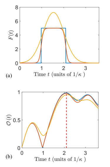
Figure 4: Comparison of three typical pulsed fields. The system is initialized in the valence bond state with $U=5\kappa$, and $F_{0}=U$. Fig. 4 (a) plots the shape of $F\left(t\right)$ and $F_{j}\left(t\right)$. Here $F\left(t\right)$ represents a square pulsed filed with $F\left(t\right)=F_{0}$ for $T/2\leqslant t\leqslant T$. The fidelity $\mathcal{O}\left(t\right)$ first oscillates because $|\underline{2}\rangle$ is not the eigenstate of the system. When the pulsed field is applied, $\mathcal{O}\left(t\right)$ approaches $1$. The only difference between such three pulsed fields is the maximum value of $\mathcal{O}\left(t\right)$, which is indicated by red dashed line. The idea case of $\mathcal{O}\left(t\right)=1$ requires: the interaction $U$ is large enough such that $|\underline{2}\rangle$ is the eigenstate of $H_{\mathrm{o}}$; the resonant pulsed filed $F_{0}=U$; the exact duration time $T/2$. It can be shown that these two types of the pulsed filed can fulfill the task that excites the system to the CDW state although $F_{j}\left(t\right)$ does not fully meet these conditions.

When we consider a Peierls distorted chain such that the nearest-neighbor hopping of $H_{\mathrm{o}}$ is staggered, the GS still has quantum number $s^{2}=0$, and $s_{z}=0$ Lieb (1989). However, the strong dimerization and large $U$ prescribe that GS is the direct product of a single valence bond in each dimerized unitcell forming a valence bond solid. This guarantees that the pulsed field takes effect in each unitcell so that the double-occupied states can be prepared individually with the same duration time $T/2$. As a consequence, the system is excited to the CDW state residing in the high energy sector. We sketch this process in Fig. 1 for clarity. This dynamical process plays a vital role in the formation of the non-equilibrium superconducting state. In the later section, we will show that such a state can develop into a superconducting state.

II.2 doublon dynamics

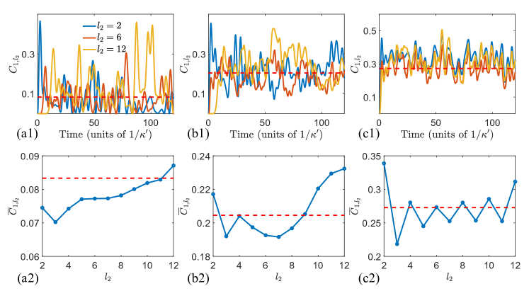
Figure 5: (a1)-(c1) Time evolution of the correlations $C_{l_{1},l_{2}}\left(t\right)$ for $2$, $6$ and $12$ filled particles of $12$-site Hubbard model. (a2)-(c2) The averaged doublon-doublon correlators $\overline{C}_{1,l_{2}}$ as function of $l_{2}$. For simplicity, $l_{1}$ is assumed to be $1$ and $l_{2}$ takes the values of $2$, $6$, and $12$ for (a1)-(c1), respectively. The initial states are chosen as $|\psi\left(0\right)\rangle=\eta_{1}^{+}|\mathrm{Vac}\rangle$, $\eta_{1}^{+}\eta_{3}^{+}\eta_{5}^{+}|\mathrm{Vac}\rangle$, and $\eta_{1}^{+}\eta_{3}^{+}\eta_{5}^{+}\eta_{7}^{+}\eta_{9}^{+}\eta_{11}^{+}|\mathrm{Vac}\rangle$. The red lines of (a)-(c) obtained by Eq. (15) serve as the benchmark to show whether the system is in the non-equilibrium superconductivity phase. It is shown that the correlator first quickly approaches the value of Eq. (15) and then it oscillates around the red line. Such dynamic behavior is independent of $l_{2}$, which indicates that the system reaches the superconducting phase featured by the emergence of the steady state with ODLRO. The unit of time $t$ is the inverse effective hopping rate $1/\kappa^{\prime}$ and the duration time $\tau$ of Figs. 5(a2)-(c2) is assumed as $240/\kappa^{\prime}$.

The dynamics of a spatially extended system of strongly correlated fermions poses a notoriously complex many-body problem that is hardly accessible to exact analytical or numerical methods. In this section, we first study the single doublon dynamics in a uniform Hubbard model, which may shed light on multi-doublon dynamics in the subsequently proposed scheme. To begin with, we assume that the two fermions are initially at the same site $j_{0}$, i.e., $|\psi_{i}\rangle=c_{j_{0},\uparrow}^{\dagger}c_{j_{0},\downarrow}^{\dagger}|\mathrm{Vac}\rangle$. Two fermions occupying the same site with strongly repulsive interaction $U$ form a doublon manifested by the fact that the total double occupancy $D=\sum_{j}\langle D_{j}\rangle$ stays near $1$. The corresponding local double-occupation operator is given by $D_{j}=n_{j,\uparrow}n_{j,\downarrow}$. It is a long-living excitation, the decay of which is suppressed because of energy conservation Hofmann and Potthoff (2012). Hence, in the large $U$ limit, the doublon dynamics can be fully captured by the following effective $\eta$-spin model, in powers of $\kappa/U$:

$$H_{\mathrm{eff}}=-\kappa^{\prime}\sum_{j}(\bm{\eta}_{j}\cdot\bm{\eta}_{j+1}-\frac{1}{4})$$ (14)

which is obtained by a unitary transformation to project out the energetically well separated high-energy part of the spectrum Fazekas (1999). In its essence, a small cluster is enough to capture the feature of doublon movement and doublon-doublon interaction due to the absence of the long-range coupling. One can safely extend the result to a large system. In Appendix A, a simple two-site case is provided to elucidate this mechanism. Note that we neglect the energy base $mU$ compared with Eq. (39) in Appendix. Here, $\kappa^{\prime}=4\kappa^{2}/U$ and $\bm{\eta}_{j}=(\eta_{j}^{x},$ $\eta_{j}^{y},$ $\eta_{j}^{z})$. For the repulsive interaction, $H_{\mathrm{eff}}$ describes a $\eta$-spin ferromagnetic model, the ground state of which is $\eta$-pairing state with the form of $|\psi_{\mathrm{eff}}^{\mathrm{g}}\left(M\right)\rangle=\left(\eta^{+}\right)^{M}/\sqrt{\Omega}|\mathrm{Vac}\rangle$ where $M$ denotes the filled number of doublons and the normalization efficient is $\Omega=C_{N}^{M}$. The discussion about the uniform Hubbard model is instructive for the effective Hamiltonian based on the dimerized Hubbard model in the subsequent section since dimerization does not alter the property of GS according to Lieb theorem Lieb (1989). It is worthy pointing out that such paring ground state usually relates to the superconductivity of the system due to the following $j$-independent correlation relation Tindall et al. (2019); Yang (1989)

$$|\langle\psi_{\mathrm{eff}}^{\mathrm{g}}\left(M\right)|\eta_{i}^{+}\eta_{i+j}^{-}|\psi_{\mathrm{eff}}^{\mathrm{g}}\left(M\right)\rangle|=\left\{\begin{array}[]{c}\frac{M(N-M)}{N(N-1)}\text{, for }j\neq 0\\ \frac{M}{N}\text{, for }j=0\end{array}\right..$$ (15)

It is also served as the building block to realize ODLRO state in the subsequent non-equilibrium dynamic scheme. To gain further insight, we first focus on the single-doublon case such that $\sum_{j}\eta_{j}^{z}\eta_{j+1}^{z}$ only provides an energy base and plays no effect on the dynamics. Hence, Eq. (14) takes the form of the tight-binding model with the effective hopping $-\kappa^{\prime}/2$, that is

$$H_{\mathrm{eff}}=-\frac{\kappa^{\prime}}{2}\sum_{j}(\eta_{j}^{+}\eta_{j+1}^{-}+\eta_{j}^{-}\eta_{j+1}^{+}).$$ (16)

Performing the open boundary condition, the resulting free tight-binding Hamiltonian is diagonalized by a simple transformation (see Appendix B for more details). According to the Appendix B, one can readily obtain the evolved state as

$$|\psi\left(t\right)\rangle=\sum_{j}g\left(j_{0},j,t\right)\eta_{j}^{+}|\mathrm{Vac}\rangle,$$ (17)

with

$$g\left(j_{0},j,t\right)=\sum_{l=-\infty}^{\infty}i^{C_{l.j_{0},j}^{1}}\mathcal{J}_{C_{l.j}^{1}}\left(2\kappa^{\prime}t\right)-i^{C_{l.j_{0},j}^{2}}\mathcal{J}_{C_{l.j}^{2}}\left(2\kappa^{\prime}t\right),$$ (18)

and

$$C_{l.j_{0},j}^{1} = j-j_{0}+lN+1,$$ (19)

$$C_{l.j_{0},j}^{2} = j-1+j_{0}+\left(l-1\right)N,$$ (20)

where $\mathcal{J}_{l}$ denotes the $l$th Bessel function of the first kind. We concentrate on the property of the evolved state after a long time scale. To this end, two physical quantities are employed to characterize $|\psi\left(t\right)\rangle$. The first is the expectation value of $d_{l}^{\dagger}d_{l}$ which can be given as

$$\overline{D}_{l}=\frac{1}{\tau}\int_{0}^{\tau}D_{l}\left(t\right)\mathrm{d}t\text{,}$$ (21)

where $D_{l}\left(t\right)=\left\langle\psi\left(t\right)\right|d_{l}^{\dagger}d_{l}|\psi\left(t\right)\rangle$ represents the doublon occupancy per site and $d_{l}^{\dagger}=c_{l,\uparrow}^{\dagger}c_{l,\downarrow}^{\dagger}$. Here $\tau$ characterizes the relaxation time that the system reaches to the steady state. The second is the averaged doublon-doublon correlation

$$\overline{C}_{l_{1},l_{2}}=\frac{1}{\tau}\int_{0}^{\tau}C_{l_{1},l_{2}}\left(t\right)\mathrm{d}t\text{,}$$ (22)

where $C_{l_{1},l_{2}}\left(t\right)=|\left\langle\psi\left(t\right)\right|\eta_{l_{1}}^{\dagger}\eta_{l_{2}}|\psi\left(t\right)\rangle|$. Note that the Eq. (15) can be employed as a benchmark to examine whether the system reaches the superconductivity. Straightforward algebra shows that $\overline{D}_{l}=1/\left(N+1\right)$ that is irrelevant to the location of the initial state $j_{0}$. It also indicates that the doublon is evenly distributed on each lattice site. Hence, one can expect that $\overline{C}_{l_{1},l_{2}}$ is independent of the relative distance between the two doublons. Due to the complexity of the analytical solution of $\overline{C}_{l_{1},l_{2}}$, we fix $l_{1}=1$ and examine the value of $\overline{C}_{1,l_{2}}$ as a function of $l_{2}$ in Fig. 5. It is shown that $\overline{C}_{1,l_{2}}$ does not depend on $l_{2}$. As the increase of the number of the doublons, the correlator $\overline{C}_{1,l_{2}}$ still stays at a constant value, that is almost $\overline{D}_{l}=M/\left(N+1\right)$, manifesting that the result is not only applicable to the case of dilute doublon gas. Figs. 5(a1)-(c1) clear show that the correlations oscillate around the red lines. The values of those lines are $0.0833$, $0.2045$, and $0.2727$, respectively, which are obtained by setting $M=1$, $3$, $6$ and $N=12$ in the Eq. (15). This indicates that such a non-equilibrium system can favor the existence of the steady ODLRO state $|\psi_{\mathrm{eff}}^{\mathrm{g}}\left(M\right)\rangle$ on a long time scale in which $\eta$-pairing mechanism plays a vital role. Such a feature is exactly what makes the system superconducting. In addition, we can also see that the system needs a certain relaxation time to enter into the non-equilibrium superconducting phase in Fig. 5. In such a dynamic process, the doublons gradually diffuse throughout the whole lattice and finally forms a stead state with a long-range correlation manifested by the oscillation of the correlator around the red line. For the Hubbard model at half-filling in Fig. 5(c), one can roughly infer that such duration time is $4N/\kappa^{\prime}$, which will be used to estimate the time scale of the subsequent dynamical scheme. So far we have demonstrated the dynamic mechanism that can generate the superconducting state from the Mott insulator phase via pulsed field. In what follows, we will propose a scheme to prepare the ODLRO state based on the dimerized Hubbard model.

III Scheme to preparing and detecting the ODLRO state

In this section, we concentrate on how to generate the ODLRO state via out-of-equilibrium dynamics based on the SSH Hubbard model. Further, we propose a dynamic method of detecting such non-equilibrium superconducting phase.

III.1 Dynamical preparing of the ODLRO state

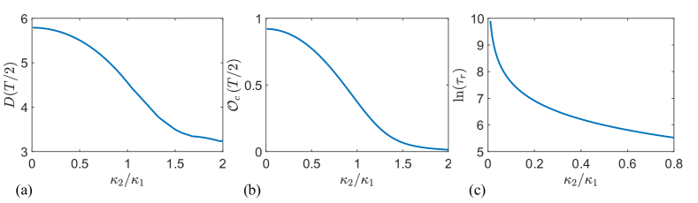
Figure 6: Plots of $D\left(T/2\right)$, $\mathcal{O}_{c}\left(T/2\right)$, and $\tau_{r}$ as a function of $\kappa_{2}/\kappa_{1}$ for the system $H^{\mathrm{d}}$ with $12$ sites. The system is initialized in the GS of a half-filled dimerized Hubbard model. The system parameters are $U=5\kappa_{1}$, and $F=U$. It is shown that the increase of $\kappa_{2}/\kappa_{1}$ decreases $D\left(T/2\right)$, and $\mathcal{O}_{c}\left(T/2\right)$, respectively. It indicates that the initial state cannot be excited to the high-energy sector of $H_{\mathrm{o}}^{\mathrm{d}}$ such that the effective Hamiltonian $H_{\mathrm{eff}}^{\mathrm{d}}$ does not hold for the evolved state when $t>T/2$. The degree of dimerization affects the relaxation time $\tau_{r}$. The stronger the dimerization the longer the relaxation time. Hence, one needs to choose a suitable intercell coupling to generate a steady superconducting state.

According to the two dynamic mechanisms proposed above, we will give the method of generating ODLRO state through the dimerized Hubabrd model. The considered $1$D time-dependent Hamiltonian can be given as

$$H^{\mathrm{d}}=H_{\mathrm{o}}^{\mathrm{d}}+H_{\mathrm{e}}^{\mathrm{d}},$$ (23)

where

$$H_{\mathrm{o}}^{\mathrm{d}} = -\sum_{j=1}^{N-1}\sum_{\sigma=\uparrow,\downarrow}(\kappa_{1}c_{2j-1,\sigma}^{\dagger}c_{2j,\sigma}$$ (24)

$$+\kappa_{2}c_{2j-1,\sigma}^{\dagger}c_{2j,\sigma}+\text{{H.c.}})$$

$$+U\sum_{j=1}^{2N}n_{j,\uparrow}n_{j,\downarrow},$$

$$H_{\mathrm{e}}^{\mathrm{d}} = F\left(t\right)\sum_{j=1}^{2N}\sum_{\sigma=\uparrow,\downarrow}jn_{j,\sigma},$$ (25)

with

$$F\left(t\right)=\left\{\begin{array}[]{c}U,\text{ }0<t\leqslant T/2\\ 0,\text{ otherwise}\end{array}\right..$$ (26)

When $U=0$, Eq. (24) reduces to a celebrated Su-Schrieffer-Heeger model that is a paradigm for characterizing the topology. Here, $\kappa_{1}/\kappa_{2}$ ratio controls the type of dimerization. In the OBC, we concentrate on the GS property of $H_{\mathrm{o}}^{\mathrm{d}}$ and do not concern the edge state behavior. Considering $H_{\mathrm{o}}^{\mathrm{d}}$ at half-filling, the GS $|\psi_{\mathrm{d}}^{\mathrm{g}}\rangle$ of $H_{\mathrm{o}}^{\mathrm{d}}$ possesses the dimerized behavior if $\kappa_{1}>\kappa_{2}$, which can be shown in Fig. 1. However, two end sites are not paired if $\kappa_{1}<\kappa_{2}$. In the extreme case of $\kappa_{1}/\kappa_{2}\gg 1$, the GS is fully dimerized and become a valence bond solid. When the tilted field is applied, each dimerized sector respects the dynamical mechanism developed in the subsection 3. As a consequence, the valence bond solid state $|\Phi\left(0\right)\rangle=|\psi_{\mathrm{d}}^{\mathrm{g}}\rangle$ will evolve to a CDW state, that is $|\Phi\left(T/2\right)\rangle=|\psi_{\mathrm{CDW}}\rangle$. For clarity, this dynamical behavior is illustrated in Fig. 1. This is the law that the evolved state should follow in an ideal case. In practice, one can neither cut off the inter-cell coupling nor increase the on-site interaction to the infinity. It can be envisioned that the presence of the inter-cell coupling suppresses the dimerization and hence leads to the reduction of the component of $|\psi_{\mathrm{CDW}}\rangle$ in the evolved state. To check this point, we plot the overlap $\mathcal{O}_{c}\left(t\right)=|\langle\Phi\left(t\right)|e^{-iH^{\mathrm{d}}t}|\psi_{\mathrm{CDW}}\rangle|$ for different values of $\kappa_{2}/\kappa_{1}$ in Fig. 6. It is shown that $D\left(T/2\right)$ and $\mathcal{O}_{c}\left(T/2\right)$ decrease as intercell-coupling increases. This indicates that the GS is not excited to the high-energy sector even though the resonant tilted field $F$ is applied. To ensure the success of the proposed scheme, one needs to choose a small inter-cell coupling such that the quantity $\mathcal{O}_{c}\left(t\right)$ approaches $1$. However, a small enough $\kappa_{2}$ also brings other drawbacks, which will be seen later.

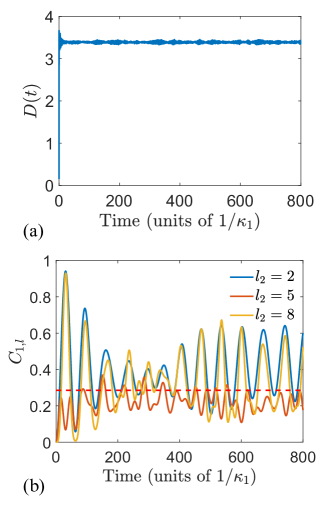
Figure 7: (a1)-(c1) Upper panel: Time evolutions of total double occupancy $D\left(t\right)$. Lower panel: Time evolutions of $\eta$ correlators $C_{1,2}\left(t\right)$, $C_{1,5}\left(t\right)$, and $C_{1,8}\left(t\right)$. The red line denotes the correlation of $\eta$-pairing state $|\psi_{\mathrm{eff}}^{\mathrm{g}}\left(M\right)\rangle$ with $M=4$, which is served as a benchmark. The system is initialized in the ground state of $H_{\mathrm{o}}^{\mathrm{SSH}}$ that is a $8$-site $1$D SSH Hubbard model at half filling with $U=10\kappa_{1}$, and $\kappa_{2}=0.5\kappa_{1}$. Under the action of the resonant pulsed field, $D\left(t\right)$ first increases rapidly to the peak, and then decays to $3.6$ followed by an almost constant trend. The tiny fluctuations around the constant “final” value are simply reflecting the fact that the total double occupancy does not commute with the Hamiltonian. Such the constant value is determined by the degree of the dimerization and guarantees the validity of our analytical analysis in the main text. After the quench, the evolved state acquires the long-range correlation in the sense that the correlator $C_{1,8}\left(t\right)$ oscillates around $0.3$. Note that the time $t$ is measured in units of the inverse hopping $1/\kappa_{1}$.

When $t>T/2$, the dynamics of $|\Phi\left(t>T/2\right)\rangle$ is only govern by $H_{\mathrm{o}}^{\mathrm{d}}$. According to the mechanism shown in the subsection 5, one can expect that the system will drive the CDW state into a ODLRO state. The only difference lies in the effective Hamiltonian regarding the doublon dynamics. It is a dimerized instead of a uniform $\eta$-spin model that can be given as

$$H_{\mathrm{eff}}^{\mathrm{d}} = -\kappa_{1}^{\prime}\sum_{j=1}^{N-1}(\bm{\eta}_{2j-1}\cdot\bm{\eta}_{2j}-\frac{1}{4})$$ (27)

$$-\kappa_{2}^{\prime}\sum_{j=1}^{N-1}(\bm{\eta}_{2j}\cdot\bm{\eta}_{2j+1}-\frac{1}{4}),$$

where $\kappa_{j}^{\prime}=4\kappa_{j}^{2}/U$. However, such staggered coupling coefficients do not alter the magnetic property of the system and hence the corresponding ground state is still a $\eta$-spin ferromagnetic state. This minor difference does not change the final steady state but only affects the relaxation time due to the inhomogeneous effective hopping $\kappa_{j}^{\prime}$ which prohibits the diffusion of the doublon in the entire lattice. For clarity, we plot the relaxation time $\tau_{r}$ as a function of $\kappa_{2}/\kappa_{1}$ in Fig. 6. Here the relaxation time refers to the duration of time that the system experiences when physical observables $\overline{C}_{l_{1},l_{2}}$, and $\overline{D}_{l}$ do not vary with time. This time is in proportion to $U/\kappa_{2}^{2}$, which can be understood by the effective Hamiltonian $H_{\mathrm{eff}}^{\mathrm{d}}$. Although the strong dimerization can ensure the main component of the final state is $|\psi_{\mathrm{CDW}}\rangle$, the relaxation time is much longer than the condition of weak dimerization due to the effective intercell hopping $U/\kappa_{2}^{2}$. Evidently, the relaxation time is infinite when the system is fully dimerized ($\kappa_{2}=0$). Given all of that, the formation of the non-equilibrium superconducting state is a trade-off. On the one hand, the strong dimerization ($\kappa_{1}/\kappa_{2}\gg 1$) ensures that the GS of $H_{\mathrm{o}}^{\mathrm{d}}$ mainly consists of the valence bond solid. Therefore, the combination of pulsed field and dimerized Hubbard model can evolve the initial ground state to a CDW state which paves the way to preparing the non-equilibrium ODLRO state. However, the cost is to significantly suppress the effective hopping between the different dimerized unit cells leading to a very long relaxation time. On the other hand, if one decreases the degree of dimerization to $\kappa_{1}\approx\kappa_{2}$, the main constituent of the GS is the Neel state although the system is still in the Mott insulating phase. Such an initial GS cannot be driven to the CDW state even though a resonant pulsed field is applied. Therefore, the non-equilibrium superconducting phase fails to achieve. In this point of view, the selection of hopping coefficient is a tradeoff between the efficiency of the proposed scheme and the duration time.

In Fig. 7, we demonstrate this dynamical scheme by setting $\kappa_{1}/\kappa_{2}=2$. In this setting, the portion of the valence-bond-solid state in the GS is about $0.9$. Hence, after a resonant pulsed field, the expectation value $\sum_{l}D_{l}\left(t\right)$ of the target state is approximately $3.6$. Fig. 7(a) clearly shows that the total double occupancy quickly approaches $3.6$ and is stabilized around that value protected by the energy conservation. Such long-lived excitation guarantees the validity of the effective $\eta$-spin ferromagnetic model in the subsequent doublon-diffusion dynamics. Consequently, the long-range correlation of $\eta$ spin is established as shown in Fig. 7(b). To give a panoramic view of the dynamical scheme, we also perform the numerical simulation in Fig. 8 to show the time evolutions of $\overline{D}_{l}$ and $\overline{C}_{1,l_{2}}$. It can be shown that the final steady state distributes evenly in the entire lattice with $\overline{D}_{l}=M/(N+1)$. This indicates the uniform diffusion of the doublons over the lattice. Furthermore, the averaged correlator $\overline{C}_{1,l}$ oscillates around $0.28$ suggesting that the system enters into the non-equilibrium superconducting phase, which verifies the previous analysis. In experiment, the proposed scheme could be implemented in the ultracold atoms loaded in optical lattices Jünemann et al. (2017); Abanin et al. (2019). The tunability and long coherence times of this system, along with the ability to prepare highly nonequilibrium states, enable one to probe such quantum dynamics.

III.2 Dynamical detection of the non-equilibrium superconducting phase

To further capture the superconductivity of the non-equilibrium system, we introduce the LE, which is a measure of reversibility and sensitivity to the perturbation of quantum evolution. The perturbation considered in our scheme is the magnetic flux threading the ring. To this end, an additional quench process should be implemented. The corresponding post-quench Hamiltonian can be given as

$$H_{\mathrm{p}}^{\mathrm{b}} = -\sum_{j=1}^{N}\sum_{\sigma=\uparrow,\downarrow}(\kappa_{1}e^{i\phi}c_{2j-1,\sigma}^{\dagger}c_{2j,\sigma}$$ (28)

$$+\kappa_{2}e^{i\phi}c_{2j,\sigma}^{\dagger}c_{2j+1,\sigma}+\text{{H.c.}})$$

$$+U\sum_{j=1}^{N}n_{j,\uparrow}n_{j,\downarrow},$$

where $c_{2N+j,\sigma}=c_{j,\sigma}$, and $\phi=2N\phi$ denotes the total magnetic flux piercing the ring. Taking the steady state $|\Phi\left(t_{f}\right)\rangle$ as an initial state, the LE is defined as

$$\mathcal{L}\left(t\right)=|\langle\Phi\left(t_{f}\right)|e^{-iH_{\mathrm{p}}^{\mathrm{b}}t}e^{iH_{\mathrm{o}}^{\mathrm{b}}t}|\Phi\left(t_{f}\right)\rangle|^{2},$$ (29)

where $t_{f}$ is relaxation time of the first quench dynamics. Eq. (29) represents the overlap at time $t$ of two states evolved from $\left|\Phi\left(t_{f}\right)\right\rangle$ under the action of the Hamiltonian operators $H_{\mathrm{o}}^{\mathrm{b}}$ and $H_{\mathrm{p}}^{\mathrm{b}}$. Consider a typical case $\kappa_{1}\sim\kappa_{2}$, the GS of $H_{\mathrm{o}}^{\mathrm{d}}$ at half-filling is an anti-ferromagnetic state. The resonant pulsed field $H_{\mathrm{e}}^{\mathrm{d}}$ does not induce the particle pairing and hence cannot place the evolved state $|\Phi\left(t_{f}\right)\rangle$ in the high-energy sector of $H_{\mathrm{o}}^{\mathrm{d}}$. It is still an insulating state residing in the low-energy sector and its dynamics is described by the effective Heisenberg Hamiltonian

$$H_{\mathrm{eff}}^{\mathrm{s}} = -\kappa_{1}^{\prime}\sum_{j=1}^{N}(\bm{s}_{2j-1}\cdot\bm{s}_{2j}-\frac{1}{4})$$ (30)

$$-\kappa_{2}^{\prime}\sum_{j=1}^{N}(\bm{s}_{2j}\cdot\bm{s}_{2j+1}-\frac{1}{4}).$$

Because of the virtual exchange of particles, this Hamiltonian does hold regardless of the presence or absence of the magnetic field. As a consequence, the post- and before-quench Hamiltonians share the same effective Hamiltonian $H_{\mathrm{eff}}^{\mathrm{s}}$ such that $\mathcal{L}\left(t\right)$ stay at $1$. Now we switch gear to another typical case $\kappa_{1}/\kappa_{2}\gg 1$ in which the steady state $|\Phi\left(t_{f}\right)\rangle$ resides in the high-energy sector due to the resonant pulsed field. It is a superconducting state featured by the constant $\eta$-spin correlator. With the same spirit, one can obtain the effective post-quench Hamiltonian in such a sector when the magnetic field is applied. According to the Appendix A, it can be given as

$$H_{\mathrm{eff}}^{\mathrm{p}} = -\frac{\kappa_{1}^{\prime}}{2}\sum_{j=1}^{N}(e^{i2\phi}\eta_{2j-1}^{+}\eta_{2j}^{-}+\text{{H.c.}}$$ (31)

$$+2\eta_{2j-1}^{z}\eta_{2j}^{z}-\frac{1}{2})$$

$$-\frac{\kappa_{2}^{\prime}}{2}\sum_{j=1}^{N}(e^{i2\phi}\eta_{2j}^{+}\eta_{2j+1}^{-}+\text{{H.c.}}$$

$$+2\eta_{2j}^{z}\eta_{2j+1}^{z}-\frac{1}{2}),$$

where the phase factor $e^{i2\phi}$ stems from the doublon hopping. This ensures that the system can respond to the external magnetic field, and hence $\mathcal{L}\left(t\right)$ changes. Note that when $\phi=n\pi$, the effective post- and before-quench Hamiltonians are the same as each other resulting in $\mathcal{L}\left(t\right)=1$. If we fix the reversal time $t=\tau$, the value of $\mathcal{L}\left(\tau\right)$ will show a periodical behavior as $\phi$ varies. In this sense, whether the LE exhibits periodic behavior is an important feature to mark whether the particles move in pairs. To confirm this conclusion, a numerical simulation of average $\overline{\mathcal{L}}$ defined as

$$\overline{\mathcal{L}}=\frac{1}{\tau}\int_{0}^{\tau}|\langle\Phi\left(t_{f}\right)|e^{-iH_{\mathrm{p}}^{\mathrm{b}}t}e^{iH_{\mathrm{o}}^{\mathrm{b}}t}|\Phi\left(t_{f}\right)\rangle|^{2}\mathrm{d}t$$ (32)

is performed in Fig. 9. It is shown that when $\kappa_{2}/\kappa_{1}=0.3$, $\overline{\mathcal{L}}\left(\phi\right)$ exhibits an oscillation with period $\phi=\pi$, which agrees with our prediction. On the contrary, $\overline{\mathcal{L}}\left(\phi\right)$ stays at $1$ if $\kappa_{2}/\kappa_{1}=1$ indicating that system is still in the Mott insulating phase. This scheme suggests an alternative dynamical approach to detecting the non-equilibrium phase of matter.

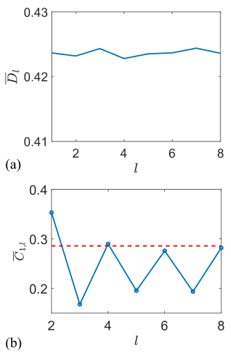
Figure 8: Numerical results for the averaged $\overline{C}_{1,l}$ and $\overline{D}_{l}$. The corresponding duration time $\tau$ is chosen as $2000/\kappa_{1}$. The other system parameters are the same as those in Fig. 8. $\overline{D}_{l}$ is evenly distributed on each lattice site leading to $l$-independent $\eta$-spin correlation. Note that the red line denotes the correlation of the $\eta$-pairing state $|\psi_{\mathrm{eff}}^{\mathrm{g}}\left(M\right)\rangle$ with $M=4$. Evidently, the steady superconducting state is prepared via non-equilibrium dynamics.

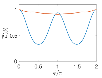
Figure 9: The average LE ($\overline{\mathcal{L}}$) for different intercell couplings with resonant pulsed field $F$. The simulation is performed in a $12$-site Hubbard model at half-filling with $s^{z}=0$, and the total magnetic flux penetrating the 1D ring is taken as $12\phi$. The red and blue lines denote $\kappa_{2}/\kappa_{1}=0.3$, and $1$, respectively. The other system parameters are $U=10\kappa_{1}$, and $t_{f}=1200/\kappa_{1}$. For the uniform chain, the final evolved state lies in the low-energy sector of $H_{\mathrm{p}}^{\mathrm{b}}$ and $H_{\mathrm{o}}^{\mathrm{d}}$. Correspondingly, the effective Heisenberg Hamiltonians of both systems share the same form as shown in Eq. (30). Hence, the average LE ($\overline{\mathcal{L}}$) does not respond to the magnetic flux. For the strong dimerization, the resonant pulse field can fully drive the valence-bond-solid state into a CDW state. Its dynamics can be captured by $\eta$-spin Hamiltonian (31) rather than Heisenberg Hamiltonian (30). When a doublon moves, it acquires a $2\phi$ phase factor that can be witnessed by the decrease of $\mathcal{L}\left(t\right)$. However, when $\phi=\pi$, the two effective Hammiltonians $H_{\mathrm{eff}}^{\mathrm{p}}$ and $H_{\mathrm{eff}}^{\mathrm{d}}$ are the same so that $\mathcal{L}\left(t\right)$ returns to $1$. In this sense, the periodical oscillation behavior of $\overline{\mathcal{L}}\left(\phi\right)$ may serve as a dynamical signature to probe whether the systems enters into the non-equilibrium superconducting phase.

IV Summary

In summary, we have proposed a non-equilibrium method to realize the long-living superconductivity in the dimerized Hubbard model. The underlying mechanism can be dissected into two main dynamical processes, dynamical pairing and doublon dynamics in the highly-excited subspace. Specifically, the dimerization in the Hubbard model makes the main component of the anti-ferromagnetic ground state change from Neel state to a valence bond solid. Therefore, the dynamical pairing is confined to each unitcell such that the corresponding valence bond state is excited to the doublon state forming the so-called CDW state. When the external field is switched off, the energy conservation prevents the decay of the doublon and hence protects such the long-lived excitation. The dynamics of the CDW state is determined by the highly-excited state of the dimerized Hubbard model, which can be described by a Heisenberg-like $\eta$-spin ferromagnetic model. After a long-time evolution, the doublons tend to distribute evenly in the entire lattice and form a steady state with ODLRO. Furthermore, we propose a dynamical detection method to identify this non-equilibrium superconducting phase via introducing the magnetic flux to trigger a quench and measuring the LE. Our results open a new avenue toward enhancing and detecting superconductivity through non-equilibrium dynamics.

Appendix A Simple example of two-site case for the effective Hamiltonian $H_{\mathrm{eff}}$

In this section, our goal is to obtain the effective Hamiltonian (14). To this end, we first divide the Hamiltonian $H_{\mathrm{o}}$ into two parts $H_{\mathrm{o}}=H_{0}+H_{t}$, where

$$H_{0} = U\sum_{j=1}n_{j,\uparrow}n_{j,\downarrow},$$ (33)

$$H_{t} = -\kappa\sum_{\sigma,j}(c_{j,\sigma}^{\dagger}c_{j+1,\sigma}+\text{H.c.}).$$ (34)

To second order in perturbation theory, the effective Hamiltonian is given by

$$H_{\mathrm{eff}}=P_{0}H_{0}P_{0}+P_{0}H_{t}P_{1}\frac{1}{E_{0}-H_{0}}P_{1}H_{t}P_{0}+O\left(\frac{\kappa^{3}}{U^{2}}\right),$$ (35)

where $P_{0}$ is a projector onto the Hilbert subspace in which there are $m$ lattice sites occupied by two particles with opposite spin orientation, and $P_{1}=1-P_{0}$ is the complementary projection. Here the energy $E_{0}$ of the unperturbed state is set to $E_{0}=mU$ where $m$ denotes the number of doublons. Since $H_{t}$ acting on states in $P_{0}$ annihilates only one double occupied site, all states in $P_{1}H_{t}P_{0}$ have exactly $m-1$ doubly occupied sites. Now we provide a detailed calculation of the two-site case for the effective Hamiltonian $H_{\mathrm{eff}}$ which may shed light to obtain the effective Hamiltonian (14). In the simplest two-site case, $P_{0}=\sum_{\alpha\in\text{{d.o.}}}|\alpha\rangle\langle\alpha|$ is the projection operator to the doublon subspace spanned by the configuration $\left\{|\text{{x}}0\rangle,|0\text{{x}}\rangle\right\}$, and $P_{1}=1-P_{0}=\sum_{a\notin\text{{d.o.}}}|a\rangle\langle a|$ is the complementary projection. Here the abbreviation d.o. means the doubly occupied subspace and $|$x$0\rangle=c_{1,\uparrow}^{\dagger}c_{1,\downarrow}^{\dagger}|$Vac$\rangle$, $|0$x$\rangle=c_{2,\uparrow}^{\dagger}c_{2,\downarrow}^{\dagger}|$Vac$\rangle$. The first term of Eq. (35) clear gives $P_{0}H_{0}P_{0}=U$. The second term can be simplified by noting: (i) the unperturbed energy $E_{0}$ is $U$; (ii) $P_{1}H_{t}P_{0}$ annihilates the doubly occupied site. Then $H_{\mathrm{eff}}^{2}$ for two-site Hubbard system can be written as

$$H_{\mathrm{eff}}^{2} = U+\sum_{\alpha,\beta\in\text{d.o.}}\sum_{a,b\notin\text{d.o.}}|\alpha\rangle\langle\alpha|H^{\prime}|a\rangle\langle a|$$ (36)

$$\times\frac{1}{U-H_{0}}|b\rangle\langle b|H^{\prime}|\beta\rangle\langle\beta|$$

$$= U+\frac{1}{U}\sum_{\alpha,\beta\in\text{d.o.}}\langle\alpha|\left(H^{\prime}\right)^{2}|\beta\rangle|\alpha\rangle\langle\beta|.$$

The second term describes the virtual exchange of the fermions yielding that

$$H_{\mathrm{eff}}^{2}=U+\frac{2\kappa^{2}}{U}\left(|\text{{x}}0\rangle\langle 0\text{{x}}|+|0\text{{x}}\rangle\langle\text{{x}}0|+|\text{{x}}0\rangle\langle\text{{x}}0|+|0\text{{x}}\rangle\langle 0\text{{x}}|\right).$$ (37)

Combining the cases in the subspaces of $|\mathrm{xx}\rangle$ and $|$Vac$\rangle$, the pseudo spin Hamiltonian can be given by the Heisenberg-like model

$$H_{\mathrm{eff}}=U-\frac{4t^{2}}{U}\left(\bm{\eta}_{1}\cdot\bm{\eta}_{2}-\frac{1}{4}\right),$$ (38)

where $\bm{\eta}_{j}=(\eta_{j}^{x},$ $\eta_{j}^{y},$ $\eta_{j}^{z})$, and $m$ can be $0$, $1$, and $2$ denoting the number of pairs of the doublon subspace. Evidently, the GS of $H_{\mathrm{eff}}$ is the $\eta$-spin ferromagnetic state with the form of $\left(\eta^{+}\right)^{2}|$Vac$\rangle$. One can extend the result to the system with $N$ sites, the corresponding effective Hamiltonian is given as

$$H_{\mathrm{eff}}=mU-\frac{4t^{2}}{U}\sum_{j}\left(\bm{\eta}_{j}\cdot\bm{\eta}_{j+1}-\frac{1}{4}\right).$$ (39)

Hence, the ferromagnetic state of $\eta$ spins aligned on the $x-y$ plane is the $\eta$-pairing superconducting state.

Appendix B The dynamics of a single doublon in a finite chain

The diffusion of the doublon on the entire lattice is the key to achieving the non-equilibrium superconducting phase of the proposed scheme. Here, we give a single doublon dynamics analytically, which may shed light on dilute doublon gas. Starting from effective Hamiltonian (16), it is a free tight-binding Hamiltonian with open boundary condition, which can be diagonalized by the following transformation

$$\eta_{k}^{+} = \sqrt{\frac{2}{N+1}}\sum_{j}\sin\left(kj\right)\eta_{j}^{+}|\mathrm{Vac}\rangle,$$ (40)

$$\eta_{k}^{-} = \sqrt{\frac{2}{N+1}}\sum_{j}\sin\left(kj\right)\eta_{j}^{-}|\mathrm{Vac}\rangle,$$ (41)

where $k=n\pi/(N+1)$. Correspondingly, the effective Hamiltonian in this representation can be given as

$$H_{\mathrm{eff}}=\sum_{k}\varepsilon_{k}\eta_{k}^{+}\eta_{k}^{-}$$ (42)

with eigen energy $\varepsilon_{k}=-\kappa^{\prime}\cos k$. Consider a double-occupied initial state with form

$$|\psi\left(t\right)\rangle=\eta_{j_{0}}^{+}|\mathrm{Vac}\rangle,$$ (43)

, one can readily obtain the evolved state in terms of operator $\eta_{k}^{+}$ as

$$|\psi\left(t\right)\rangle=\sqrt{\frac{2}{N+1}}\sum_{k}e^{-i\varepsilon_{k}t}\sin kj_{0}\eta_{k}^{+}|\mathrm{Vac}\rangle,$$ (44)

Taking the inverse transformation, the evolved state in the coordinate space is

$$|\psi\left(t\right)\rangle=\sum_{j}g\left(j_{0},j,t\right)\eta_{j}^{+}|\mathrm{Vac}\rangle,$$ (45)

where

$$g\left(j_{0},j,t\right)=\frac{2}{N+1}\sum_{k}e^{-i\varepsilon_{k}t}\sin kj\sin kj_{0},$$ (46)

can be deemed as the propagator describing how much the probability of the doublon flow from the initial $j_{0}$th to $j$th site. In the limit $N\rightarrow\infty$, the summation $\sum_{k}/N$ in Eq. (46) can be replaced by the integral $\int\mathrm{d}k$ such that

$$g\left(j_{0},j,t\right)=i^{j-j_{0}}\mathcal{J}_{j-j_{0}}\left(2\kappa^{\prime}t\right)-i^{j+j_{0}}\mathcal{J}_{j+j_{0}}\left(2\kappa^{\prime}t\right),$$ (47)

where $\mathcal{J}_{l}$ denotes the $l$th Bessel function of the first kind. However, such substitution is not true as $N$ is a finite number. As an alternative, the summation in Eq. (46) can be expanded by the Bessel function as

$$g\left(j_{0},j,t\right)=\sum_{l=-\infty}^{\infty}i^{C_{l.j_{0},j}^{1}}\mathcal{J}_{C_{l.j_{0},j}^{1}}\left(2\kappa^{\prime}t\right)-i^{C_{l.j_{0},j}^{2}}\mathcal{J}_{C_{l.j_{0},j}^{2}}\left(2\kappa^{\prime}t\right),$$ (48)

with

$$C_{l.j_{0},j}^{1} = j-j_{0}+lN+1,$$ (49)

$$C_{l.j_{0},j}^{2} = j-1+j_{0}+\left(l-1\right)N.$$ (50)

From another point of view, the dynamics in a finite chain can be obtained by projecting the dynamics of an infinite system to such a finite system. In this scenario, one can utilize safely the Bessel function to capture the interference behavior when the evolved state touches the boundary. The cost is to project the Bessel function entirely into the subsystem. The infinite summation of Eq. (48) denotes such a physical process.

References

- Verstraete et al. (2009) F. Verstraete, M. M. Wolf, and J. Ignacio Cirac, Nature Physics 5, 633 (2009), ISSN 1745-2481, URL https://doi.org/10.1038/nphys1342.
- Ichikawa et al. (2011) H. Ichikawa, S. Nozawa, T. Sato, A. Tomita, K. Ichiyanagi, M. Chollet, L. Guerin, N. Dean, A. Cavalleri, S.-i. Adachi, et al., Nature Materials 10, 101 (2011), ISSN 1476-4660, URL https://doi.org/10.1038/nmat2929.
- Eisert et al. (2015) J. Eisert, M. Friesdorf, and C. Gogolin, Nature Physics 11, 124 (2015), ISSN 1745-2481, URL https://doi.org/10.1038/nphys3215.
- Basov et al. (2017) D. N. Basov, R. D. Averitt, and D. Hsieh, Nature Materials 16, 1077 (2017), ISSN 1476-4660, URL https://doi.org/10.1038/nmat5017.
- Mor et al. (2017) S. Mor, M. Herzog, D. Golež, P. Werner, M. Eckstein, N. Katayama, M. Nohara, H. Takagi, T. Mizokawa, C. Monney, et al., Phys. Rev. Lett. 119, 086401 (2017), URL https://link.aps.org/doi/10.1103/PhysRevLett.119.086401.
- Cavalleri (2018) A. Cavalleri, Contemporary Physics 59, 31 (2018), ISSN 0010-7514, URL https://doi.org/10.1080/00107514.2017.1406623.
- Ishihara (2019) S. Ishihara, J. Phys. Soc. Jpn. 88, 072001 (2019), ISSN 0031-9015, URL https://doi.org/10.7566/JPSJ.88.072001.
- Greiner et al. (2002) M. Greiner, O. Mandel, T. W. Hänsch, and I. Bloch, Nature 419, 51 (2002), ISSN 1476-4687, URL https://doi.org/10.1038/nature00968.
- Freericks et al. (2006) J. K. Freericks, V. M. Turkowski, and V. Zlatić, Phys. Rev. Lett. 97, 266408 (2006), URL https://link.aps.org/doi/10.1103/PhysRevLett.97.266408.
- Bloch et al. (2008) I. Bloch, J. Dalibard, and W. Zwerger, Rev. Mod. Phys. 80, 885 (2008), URL https://link.aps.org/doi/10.1103/RevModPhys.80.885.
- Freericks (2008) J. K. Freericks, Phys. Rev. B 77, 075109 (2008), URL https://link.aps.org/doi/10.1103/PhysRevB.77.075109.
- Aron et al. (2012) C. Aron, G. Kotliar, and C. Weber, Phys. Rev. Lett. 108, 086401 (2012), URL https://link.aps.org/doi/10.1103/PhysRevLett.108.086401.
- Aoki et al. (2014) H. Aoki, N. Tsuji, M. Eckstein, M. Kollar, T. Oka, and P. Werner, Rev. Mod. Phys. 86, 779 (2014), URL https://link.aps.org/doi/10.1103/RevModPhys.86.779.
- Essler and Fagotti (2016) F. H. L. Essler and M. Fagotti, Journal of Statistical Mechanics: Theory and Experiment 2016, 064002 (2016), ISSN 1742-5468, URL http://dx.doi.org/10.1088/1742-5468/2016/06/064002.
- Vidmar and Rigol (2016) L. Vidmar and M. Rigol, Journal of Statistical Mechanics: Theory and Experiment 2016, 064007 (2016), ISSN 1742-5468, URL http://dx.doi.org/10.1088/1742-5468/2016/06/064007.
- Vasseur and Moore (2016) R. Vasseur and J. E. Moore, Journal of Statistical Mechanics: Theory and Experiment 2016, 064010 (2016), ISSN 1742-5468, URL http://dx.doi.org/10.1088/1742-5468/2016/06/064010.
- Wang et al. (2016) Y. Wang, B. Moritz, C.-C. Chen, C. J. Jia, M. van Veenendaal, and T. P. Devereaux, Phys. Rev. Lett. 116, 086401 (2016), URL https://link.aps.org/doi/10.1103/PhysRevLett.116.086401.
- Zhang and Song (2020) X. Z. Zhang and Z. Song, Phys. Rev. B 102, 174303 (2020), URL https://link.aps.org/doi/10.1103/PhysRevB.102.174303.
- Rubio-Abadal et al. (2020) A. Rubio-Abadal, M. Ippoliti, S. Hollerith, D. Wei, J. Rui, S. L. Sondhi, V. Khemani, C. Gross, and I. Bloch, Phys. Rev. X 10, 021044 (2020), URL https://link.aps.org/doi/10.1103/PhysRevX.10.021044.
- Moudgalya et al. (2020) S. Moudgalya, N. Regnault, and B. A. Bernevig, Phys. Rev. B 102, 085140 (2020), URL https://link.aps.org/doi/10.1103/PhysRevB.102.085140.
- Wei et al. (2021) D. Wei, A. Rubio-Abadal, B. Ye, F. Machado, J. Kemp, K. Srakaew, S. Hollerith, J. Rui, S. Gopalakrishnan, and N. Y. Yao, arXiv preprint arXiv:2107.00038 (2021).
- Zhang and Song (2022) X. Z. Zhang and Z. Song, Phys. Rev. B 105, 054302 (2022), URL https://link.aps.org/doi/10.1103/PhysRevB.105.054302.
- Perfetti et al. (2006) L. Perfetti, P. A. Loukakos, M. Lisowski, U. Bovensiepen, H. Berger, S. Biermann, P. S. Cornaglia, A. Georges, and M. Wolf, Phys. Rev. Lett. 97, 067402 (2006), URL https://link.aps.org/doi/10.1103/PhysRevLett.97.067402.
- Fausti et al. (2011) D. Fausti, R. I. Tobey, N. Dean, S. Kaiser, A. Dienst, M. C. Hoffmann, S. Pyon, T. Takayama, H. Takagi, and A. Cavalleri, Science 331, 189 (2011), URL http://science.sciencemag.org/content/331/6014/189.abstract.
- Hu et al. (2014) W. Hu, S. Kaiser, D. Nicoletti, C. R. Hunt, I. Gierz, M. C. Hoffmann, M. Le Tacon, T. Loew, B. Keimer, and A. Cavalleri, Nature Materials 13, 705 (2014), ISSN 1476-4660, URL https://doi.org/10.1038/nmat3963.
- Kaiser et al. (2014) S. Kaiser, C. R. Hunt, D. Nicoletti, W. Hu, I. Gierz, H. Y. Liu, M. Le Tacon, T. Loew, D. Haug, B. Keimer, et al., Phys. Rev. B 89, 184516 (2014), URL https://link.aps.org/doi/10.1103/PhysRevB.89.184516.
- Mitrano et al. (2016) M. Mitrano, A. Cantaluppi, D. Nicoletti, S. Kaiser, A. Perucchi, S. Lupi, P. Di Pietro, D. Pontiroli, M. Riccò, S. R. Clark, et al., Nature 530, 461 (2016), ISSN 1476-4687, URL https://doi.org/10.1038/nature16522.
- Cantaluppi et al. (2018) A. Cantaluppi, M. Buzzi, G. Jotzu, D. Nicoletti, M. Mitrano, D. Pontiroli, M. Riccò, A. Perucchi, P. Di Pietro, and A. Cavalleri, Nature Physics 14, 837 (2018), ISSN 1745-2481, URL https://doi.org/10.1038/s41567-018-0134-8.
- Yonemitsu and Nasu (2008) K. Yonemitsu and K. Nasu, Physics Reports 465, 1 (2008), ISSN 0370-1573, URL https://www.sciencedirect.com/science/article/pii/S0370157308001476.
- Giannetti et al. (2016) C. Giannetti, M. Capone, D. Fausti, M. Fabrizio, F. Parmigiani, and D. Mihailovic, Advances in Physics 65, 58 (2016), ISSN 0001-8732, URL https://doi.org/10.1080/00018732.2016.1194044.
- Oka and Kitamura (2019) T. Oka and S. Kitamura, Annu. Rev. Condens. Matter Phys. 10, 387 (2019), ISSN 1947-5454, URL https://doi.org/10.1146/annurev-conmatphys-031218-013423.
- de la Torre et al. (2021) A. de la Torre, D. M. Kennes, M. Claassen, S. Gerber, J. W. McIver, and M. A. Sentef, Rev. Mod. Phys. 93, 041002 (2021), URL https://link.aps.org/doi/10.1103/RevModPhys.93.041002.
- Suzuki et al. (2019) T. Suzuki, T. Someya, T. Hashimoto, S. Michimae, M. Watanabe, M. Fujisawa, T. Kanai, N. Ishii, J. Itatani, S. Kasahara, et al., Communications Physics 2, 115 (2019), ISSN 2399-3650, URL https://doi.org/10.1038/s42005-019-0219-4.
- Stojchevska et al. (2014) L. Stojchevska, I. Vaskivskyi, T. Mertelj, P. Kusar, D. Svetin, S. Brazovskii, and D. Mihailovic, Science 344, 177 (2014), URL http://science.sciencemag.org/content/344/6180/177.abstract.
- Matsuzaki et al. (2014) H. Matsuzaki, M. Iwata, T. Miyamoto, T. Terashige, K. Iwano, S. Takaishi, M. Takamura, S. Kumagai, M. Yamashita, R. Takahashi, et al., Phys. Rev. Lett. 113, 096403 (2014), URL https://link.aps.org/doi/10.1103/PhysRevLett.113.096403.
- Kogar et al. (2020) A. Kogar, A. Zong, P. E. Dolgirev, X. Shen, J. Straquadine, Y.-Q. Bie, X. Wang, T. Rohwer, I.-C. Tung, Y. Yang, et al., Nature Physics 16, 159 (2020), ISSN 1745-2481, URL https://doi.org/10.1038/s41567-019-0705-3.
- Murotani et al. (2019) Y. Murotani, C. Kim, H. Akiyama, L. N. Pfeiffer, K. W. West, and R. Shimano, Phys. Rev. Lett. 123, 197401 (2019), URL https://link.aps.org/doi/10.1103/PhysRevLett.123.197401.
- Yang (1989) C. N. Yang, Phys. Rev. Lett. 63, 2144 (1989), URL https://link.aps.org/doi/10.1103/PhysRevLett.63.2144.
- Kitamura and Aoki (2016) S. Kitamura and H. Aoki, Phys. Rev. B 94, 174503 (2016), URL https://link.aps.org/doi/10.1103/PhysRevB.94.174503.
- Kaneko et al. (2019) T. Kaneko, T. Shirakawa, S. Sorella, and S. Yunoki, Phys. Rev. Lett. 122, 077002 (2019), URL https://link.aps.org/doi/10.1103/PhysRevLett.122.077002.
- Tindall et al. (2019) J. Tindall, B. Buča, J. R. Coulthard, and D. Jaksch, Phys. Rev. Lett. 123, 030603 (2019), URL https://link.aps.org/doi/10.1103/PhysRevLett.123.030603.
- Fujiuchi et al. (2019) R. Fujiuchi, T. Kaneko, Y. Ohta, and S. Yunoki, Phys. Rev. B 100, 045121 (2019), URL https://link.aps.org/doi/10.1103/PhysRevB.100.045121.
- Peronaci et al. (2020) F. Peronaci, O. Parcollet, and M. Schiró, Phys. Rev. B 101, 161101 (2020), URL https://link.aps.org/doi/10.1103/PhysRevB.101.161101.
- Fujiuchi et al. (2020) R. Fujiuchi, T. Kaneko, K. Sugimoto, S. Yunoki, and Y. Ohta, Phys. Rev. B 101, 235122 (2020), URL https://link.aps.org/doi/10.1103/PhysRevB.101.235122.
- Ejima et al. (2020) S. Ejima, T. Kaneko, F. Lange, S. Yunoki, and H. Fehske, Phys. Rev. Research 2, 032008 (2020), URL https://link.aps.org/doi/10.1103/PhysRevResearch.2.032008.
- Li et al. (2020) J. Li, D. Golez, P. Werner, and M. Eckstein, Phys. Rev. B 102, 165136 (2020), URL https://link.aps.org/doi/10.1103/PhysRevB.102.165136.
- Kaneko et al. (2020) T. Kaneko, S. Yunoki, and A. J. Millis, Phys. Rev. Research 2, 032027 (2020), URL https://link.aps.org/doi/10.1103/PhysRevResearch.2.032027.
- Zhang and Song (2021) X. Z. Zhang and Z. Song, Phys. Rev. B 103, 235153 (2021), URL https://link.aps.org/doi/10.1103/PhysRevB.103.235153.
- Lieb (1989) E. H. Lieb, Phys. Rev. Lett. 62, 1201 (1989), URL https://link.aps.org/doi/10.1103/PhysRevLett.62.1201.
- Hofmann and Potthoff (2012) F. Hofmann and M. Potthoff, Phys. Rev. B 85, 205127 (2012), URL https://link.aps.org/doi/10.1103/PhysRevB.85.205127.
- Fazekas (1999) P. Fazekas, Lecture Notes on Electron Correlation and Magnetism, vol. Volume 5 (WORLD SCIENTIFIC, 1999), URL https://doi.org/10.1142/2945.
- Jünemann et al. (2017) J. Jünemann, A. Piga, S.-J. Ran, M. Lewenstein, M. Rizzi, and A. Bermudez, Phys. Rev. X 7, 031057 (2017), URL https://link.aps.org/doi/10.1103/PhysRevX.7.031057.
- Abanin et al. (2019) D. A. Abanin, E. Altman, I. Bloch, and M. Serbyn, Rev. Mod. Phys. 91, 021001 (2019), URL https://link.aps.org/doi/10.1103/RevModPhys.91.021001.