Sivers, Boer-Mulders and worm-gear distributions at next-to-leading order

Abstract

We compute the Sivers, Boer-Mulders, worm-gear (T and L) transverse momentum dependent distributions in terms of twist-two and twist-three collinear distributions in the small-$b$ limit up to next-to-leading order (NLO) in perturbation theory.

1 Introduction

The leading power transverse momentum dependent factorization theorem introduces eight quark transverse momentum-dependent distributions (TMDs) Mulders:1995dh ; Boer:1997nt ; Boer:1999uu , which are listed in table 1. Altogether, these eight TMDs provide a comprehensive description of the nucleon’s three-dimensional spin-orbital structure in momentum space. Some of these TMDs (primarily the unpolarized ones) are studied very well theoretically and experimentally (for recent developments, see Scimemi:2019cmh ; Bacchetta:2022awv ). However, several of these TMDs are still almost unexplored. This paper is devoted to study the Sivers, Boer-Mulders, worm-gear-T, and worm-gear-L (also known as Kotzinian–Mulders) functions in the limit of small-$b$ (or, equivalently, large transverse momentum) within QCD perturbation theory.

TMDs are nonperturbative functions of two kinematic variables $x$ and $k_{T}$, being $x$ the collinear momentum-fraction and $k_{T}$ the transverse momentum. Equivalently, one can use Fourier transformed TMDs $k_{T}$-space to position space, labelling the transverse coordinate vector with $b$. In many aspects, the position space definition is advantageous. We use it throughout the work, referring to the distributions depending on $x$ and $b$ as TMDs. Different ranges of $x$ and $b$ correspond to different physical pictures, relevant for different processes. In particular, in the limit of small $b$, TMDs turn into ordinary one-dimensional collinear parton distributions. Schematically, this relation has the form

$$F(x,b)=C(x,\ln(\mu b))\otimes f(x,\mu)+\mathcal{O}(b^{2}),$$ (1)

where $F$ is a TMD, $f$ is a collinear distribution, $C$ is a perturbative coefficient function, and $\otimes$ is an integral convolution. The expansion (1) (also known as the “matching relation” Collins:2011zzd ) follows from the operator product expansion (OPE) and can be derived systematically order-by-order in the coupling constant and powers of $b^{2}$ Moos:2020wvd .

Small-$b$ expansions for TMDs have been intensively studied during the last decade. Naturally, the main efforts were devoted to the unpolarized distribution $f_{1}$, for which the coefficient function is known at next-to-next-to-next-to-leading order (N³LO) in the QCD coupling constant Ebert:2020qef ; Luo:2020epw . For the other distributions, the analysis is less developed. So, the transversity $h_{1}$ and linearly-polarized gluon TMD $h^{g}_{1}$ are known up to NNLO Gutierrez-Reyes:2018iod ; Gutierrez-Reyes:2019rug . The helicity $g_{1}$ is known at NLO Gutierrez-Reyes:2017glx ; Buffing:2017mqm ; Bacchetta:2013pqa . All these TMDs are special because their small-$b$ asymptotic contains only collinear distributions of twist-two. Therefore, their computation is relatively straightforward and can be done with standard techniques. However, the majority of TMDs match collinear distributions of higher twists, making their study more cumbersome. Thus, for Boer-Mulders $h_{1}^{\perp}$, worm-gear-T $g_{1T}$, and worm-gear-L $h_{1L}^{\perp}$ the small-$b$ expansion is known only at LO Kanazawa:2015ajw ; Scimemi:2018mmi ; Meissner:2007rx ; Boer:2003cm with some partial results known at NLO Ji:2006ub ; Zhou:2009jm ; Dai:2014ala , and for the Sivers function $f_{1T}^{\perp}$ at NLO Scimemi:2019gge . The pretzelosity distribution $h_{1T}^{\perp}$ differs from other TMDs. Its leading term is given by a twist-four operator, while matching is only known for the twist-three part Moos:2020wvd . In table 1 we indicate the twists of collinear distributions that appear as the leading-power term in eqn. (1).

	U	H	T
U	$f_{1}$ (tw2)		$h_{1}^{\perp}$ (tw3)
L		$g_{1}$ (tw2)	$h_{1L}^{\perp}$ (tw2 & tw3)
T	$f_{1T}^{\perp}$ (tw3)	$g_{1T}$ (tw2 & tw3)	$h_{1}$ (tw2)
			$h_{1T}^{\perp}$ (tw3 & tw4)

Table 1: Quark TMDs sorted with respect to polarization properties of both the operator (columns) and the hadron (rows). The labels U, H, L, and T, are for the unpolarized, helicity, longitudinal, and transverse polarizations. In brackets, we indicate the twist of collinear distributions to which TMDs match at small-$b$. The blue color highlights TMDs that are investigated in this work.

The usage of matching relations is essential for practical applications. It allows incorporating the already-known parton distribution functions into TMDs, essentially increasing the predictive power of the formalism. In fact, all modern phenomenological extractions of TMDs are based on these relations (see f.i. Bacchetta:2017gcc ; Scimemi:2017etj ; Scimemi:2019cmh ; Bacchetta:2022awv ; Cammarota:2020qcw ; Echevarria:2020hpy ; Bury:2022czx ). The twist-two part of the matching relation (the so-called Wandzura-Wilczek-like (WW-like) approximation) is supposed to work fairly well for many cases Cammarota:2020qcw ; Bhattacharya:2021twu . Also, matching relations can be inverted and used to determine collinear distributions from TMDs. For example, the knowledge of Sivers function provides an essential constraint on the Qiu-Sterman twist-three distribution Bury:2021sue ; Bury:2020vhj . Finally, the relation (1) links TMD factorization theorem to resummation approach Collins:1981uk , which is vital for the description of the high-energy data. In all these cases, it is critical to employ at least NLO expressions to fix the scaling properties of distributions.

This contribution aims to close the remaining gap in the theoretical description of polarized TMDs and compute the small-$b$ expansion for TMDs with leading twist-three contributions at NLO. This includes the Sivers, Boer-Mulders, worm-gear-T, and worm-gear-L functions, highlighted in table 1.

There are several approaches to compute higher-twist contributions to the small-$b$ asymptotics of TMDs Kanazawa:2015ajw ; Sun:2013hua ; Dai:2014ala ; Scimemi:2018mmi ; Scimemi:2019gge ; Moos:2020wvd . Among them, the most practical for the present case is the method used in ref. Scimemi:2019gge , i.e. the background-field method with collinear counting. This method is a generalization of the classical approach to deep-inelastic scattering (DIS) Balitsky:1987bk . It has been used recently for many higher-twist computations including quasi- and pseudo-distributions Braun:2021aon ; Braun:2021gvv , leading and sub-leading power TMDs Scimemi:2019gge ; Vladimirov:2021hdn ; Rodini:2022wki . In many aspects, the work presented here is the straightforward generalization of the computation performed in ref. Scimemi:2019gge for different polarizations (we also recompute the Sivers function as a cross-check). Therefore, we do not provide a detailed description of the method, which can be found in the refs. Scimemi:2019gge ; Braun:2021aon together with computational examples. Instead, we provide a general discussion, emphasizing the present case’s particularities, and present the final expression.

The paper is structured as follows. In section 2, we collect the definitions of TMDs and collinear distributions – the main subjects of the present work. In section 3, we provide the essential details on the computation method (referring, for an extended discussion, to Scimemi:2019gge ; Braun:2021aon ). The generalization of $\gamma^{5}$ in $d$ dimensions and the definition of gluon correlator) are described in more detail in sections 3.3 and 3.4, respectively. In section 4, we present NLO expressions for Sivers, Boer-Mulders, and worm-gear functions in momentum-fraction space. The position space expressions (split into contributions from the different diagrams) are given in appendix B. In appendix A are collected the expressions for the twist-three evolution kernels used as cross-check of our computation.

2 Definition of distributions

In this work, we deal with many parton distributions. For clarity, we collect their definition and important properties in this section.

2.1 TMD distributions

The quark TMDs are defined for the Drell-Yan process, taken as an example, by the following matrix element

$$\Phi^{[\Gamma]}(x,b)=\frac{1}{2}\int\frac{dz}{2\pi}e^{-ixzp^{+}}\langle p,S|\bar{q}(zn+b)[zn+b,-\infty n+b]\Gamma[-\infty n,0]q(0)|p,S\rangle,$$ (2)

where $n$ is the light-like vector ($n^{2}=0$) associated with the large component of the hadron momentum $p$, $b$ is the vector tranverse to the $(p,n)$ plane, and $\Gamma$ is a Dirac matrix. $[x,y]$ is the straight Wilson lines from $x$ to $y$,

$$[a_{1}n+b,a_{2}n+b]=P\exp\left(ig\int_{a_{2}}^{a_{1}}d\sigma n^{\mu}A_{\mu}(\sigma n+b)\right).$$ (3)

The standard parameterization of the matrix element (2) can be found in ref. Mulders:1995dh . It reads

$$\Phi^{[\gamma^{+}]}(x,b) = f_{1}(x,b)+i\epsilon^{\mu\nu}_{T}b_{\mu}s_{T\nu}Mf_{1T}^{\perp}(x,b),$$ (4)

$$\Phi^{[\gamma^{+}\gamma^{5}]}(x,b) = \lambda g_{1}(x,b)+i(b\cdot s_{T})Mg_{1T}(x,b),$$ (5)

$$\Phi^{[i\sigma^{\alpha+}\gamma^{5}]}(x,b) = s_{T}^{\alpha}h_{1}(x,b)-i\lambda b^{\alpha}Mh_{1L}^{\perp}(x,b)$$

$$+i\epsilon^{\alpha\mu}b_{\mu}Mh_{1}^{\perp}(x,b)-\frac{M^{2}b^{2}}{2}\left(\frac{g_{T}^{\alpha\mu}}{2}-\frac{b^{\alpha}b^{\mu}}{b^{2}}\right)s_{T\mu}h_{1T}^{\perp}(x,b),$$

where $b^{2}<0$. Here,

$$g_{T}^{\mu\nu}=g^{\mu\nu}-n^{\mu}\bar{n}^{\nu}-\bar{n}^{\mu}n^{\nu},\qquad\epsilon^{\mu\nu}_{T}=\bar{n}_{\alpha}n_{\beta}\epsilon^{\alpha\beta\mu\nu}=\epsilon^{-+\mu\nu},$$ (7)

where $\bar{n}^{\mu}$ is light-cone vector ($\bar{n}^{2}=0$) associated with the small-component of the hadron momentum, i.e. $p^{\mu}=p^{+}\bar{n}^{\mu}+M^{2}n^{\mu}/(2p^{+})$ with $p^{+}=(n\cdot p)$. The relative normalization is $(n\cdot\bar{n})=1$. The Levi-Civita tensor and $\gamma^{5}$-matrix are defined in $4$ dimensions as

$$\epsilon^{0123}=+1,\qquad\gamma^{5}=-\frac{i}{4!}\epsilon^{\mu\nu\alpha\beta}\gamma_{\mu}\gamma_{\nu}\gamma_{\alpha}\gamma_{\beta}.$$ (8)

Consequently, $\epsilon_{T}^{12}=\epsilon_{T,12}=+1$.

The variables $\lambda$ and $s_{T}$ are longitudinal and transverse components of the spin vector

$$s^{\mu}=\lambda\frac{p^{+}\bar{n}^{\mu}}{M}-\lambda\frac{n^{\mu}M}{2p^{+}}+s_{T}^{\mu},$$ (9)

where $M$ is the mass of the hadron. This implies $\lambda=Ms^{+}/p^{+}$.

All TMDs are dimensionless real functions that depend on $b^{2}$ (the argument $b$ is used for shortness). In this work, we consider only Sivers ($f_{1T}^{\perp}$), Boer-Mulders ($h_{1}^{\perp}$), worm-gear-T ($g_{1T}$) and worm-gear-L ($h_{1L}^{\perp}$) functions.

The definition (2) in a SIDIS-like process has the Wilson line pointing to $+\infty n$ Boer:2003cm instead to $-\infty n$. The T-even TMDs (in the present context, these are the worm-gear functions, $g_{1T}$ and $h_{1L}^{\perp}$) are independent of the direction of the staple contour due to the T-invariance of QCD. They are the same for Drell-Yan-like and SIDIS-like cases. In contrast, the T-odd TMDs (Sivers $f_{1T}^{\perp}$ and Boer-Mulders $h_{1}^{\perp}$ functions) dependent on the direction of the staple contour. One has Collins:2002kn

$$f_{1T}^{\perp}(x,b)\Big{|}_{\text{DY}}=-f_{1T}^{\perp}(x,b)\Big{|}_{\text{SIDIS}},\qquad h_{1}^{\perp}(x,b)\Big{|}_{\text{DY}}=-h_{1}^{\perp}(x,b)\Big{|}_{\text{SIDIS}}.$$ (10)

Apart of the sign-change the TMDs are identical for both cases. In the following, we assume the DY-like definition, if not specified.

The bare TMDs contain two types of divergences – ultraviolet and rapidity divergences. Both types of divergences are multiplicatively renormalizable Vladimirov:2017ksc . As a consequence, the renormalized TMD depends on two scales $\mu$ and $\zeta$. These dependencies are described by the evolution equations

$$\mu^{2}\frac{dF(x,b;\mu,\zeta)}{d\mu^{2}}=\frac{\gamma_{F}(\mu,\zeta)}{2}F(x,b;\mu,\zeta),\qquad\zeta\frac{dF(x,b;\mu,\zeta)}{d\zeta}=-\mathcal{D}(b,\mu)F(x,b;\mu,\zeta),$$ (11)

where $F$ is any TMD, $\gamma_{F}$ is the TMD anomalous dimension, and $\mathcal{D}$ is the Collins-Soper kernel Collins:1981uk . At LO, these kernels are Aybat:2011zv

$$\gamma_{F}(\mu,\zeta)=a_{s}(\mu)\left(4C_{F}\mathbf{l}_{\zeta}+6C_{F}\right)+\mathcal{O}(a_{s}^{2}),\qquad\mathcal{D}(b,\mu)=a_{s}(\mu)2C_{F}\mathbf{L}_{b}+\mathcal{O}(a_{s}^{2},b^{2}),$$ (12)

where

$$a_{s}(\mu)=\frac{g^{2}}{(4\pi)^{2}},\qquad\mathbf{l}_{\zeta}=\ln\left(\frac{\mu^{2}}{\zeta}\right),\qquad\mathbf{L}_{b}=\ln\left(\frac{(-b^{2})\mu^{2}}{4e^{-2\gamma_{E}}}\right),$$ (13)

with $g$ being the QCD coupling constant, and $\gamma_{E}$ is the Euler-Mascheroni constant. In the following text, we often omit the scales $(\mu,\zeta)$ to simplify notation. These scales can be reconstructed from the context.

The relation between momentum and position space TMDs is

$$\Phi^{[\Gamma]}(x,k_{T})=\int\frac{d^{2}b}{(2\pi)}e^{-i(b\cdot k_{T})}\Phi^{[\Gamma]}(x,b),$$ (14)

where $k_{T}$ is the transverse momentum ($k_{T}^{2}<0$). The transformations for individual TMDs can be found in refs. Boer:2011xd ; Scimemi:2018mmi . The momentum-space definition is less convenient for theoretical computations. Therefore, in the following, we use only position space TMDs.

2.2 Collinear distributions of twist-two

The collinear distributions of twist-two are defined as follows (see e.g. Jaffe:1996zw )

$$\langle p,S|\bar{q}(zn)[zn,0]\gamma^{+}q(0)|p,S\rangle = 2p^{+}\int_{-1}^{1}dxe^{ixzp^{+}}f_{1}(x),$$ (15)

$$\langle p,S|\bar{q}(zn)[zn,0]\gamma^{+}\gamma^{5}q(0)|p,S\rangle = 2\lambda p^{+}\int_{-1}^{1}dxe^{ixzp^{+}}g_{1}(x),$$ (16)

$$\langle p,S|\bar{q}(zn)[zn,0]i\sigma^{\alpha+}\gamma^{5}q(0)|p,S\rangle = 2s_{T}^{\alpha}p^{+}\int_{-1}^{1}dxe^{ixzp^{+}}h_{1}(x),$$ (17)

where $\alpha$ is a transverse index. These distributions are known as unpolarized ($f_{1}$), helicity ($g_{1}$) and tranversity distributions ($h_{1}$). They are defined for $x\in[-1,1]$ and are zero for $|x|>1$. The distributions with negative $x$ are usually interpreted as distributions of antiquarks,

$$f_{1}(x) = \theta(x)f_{1,q}(x)-\theta(-x)f_{1,\bar{q}}(-x),$$

$$g_{1}(x) = \theta(x)g_{1,q}(x)+\theta(-x)g_{1,\bar{q}}(-x),$$ (18)

$$h_{1}(x) = \theta(x)h_{1,q}(x)-\theta(-x)h_{1,\bar{q}}(-x).$$

In the present work, the unpolarized distribution does not appear, and is presented here only for comparison.

Note that the notation $f_{1}$, $g_{1}$ and $h_{1}$ is the same for TMD distributions and collinear distributions. We distinguish these functions by their arguments, which are $(x,b)$ for TMDs and $(x)$ for collinear distributions.

The gluon collinear distributions are defined as

$$\langle p,S|F_{\mu+}(zn)[zn,0]F_{\nu+}(0)|p,S\rangle = (p^{+})^{2}\int_{-1}^{1}dxe^{ixzp^{+}}\frac{x}{2}\left(-g^{\mu\nu}_{T}f_{g}(x)-i\epsilon^{\mu\nu}_{T}\Delta f_{g}(x)\right),$$ (19)

where $f_{g}$ and $\Delta f_{g}$ are unpolarized and helicity gluon distributions. Gluon distributions satisfy the ralation

$$f_{g}(-x)=-f_{g}(x),\qquad\Delta f_{g}(-x)=+\Delta f_{g}(x).$$ (20)

In dimensional regularization (with $d=4-2\epsilon$) the definition of gluon distributions (19) is modified and takes the form

$$\langle p,S|F_{\mu+}(zn)[zn,0]F_{\nu+}(0)|p,S\rangle = (p^{+})^{2}\int_{-1}^{1}dxe^{ixzp^{+}}\frac{x}{2}\left(-\frac{g^{\mu\nu}_{T}f_{g}(x)}{1-\epsilon}-\frac{i\epsilon^{\mu\nu}_{T}\Delta f_{g}(x)}{(1-\epsilon)(1-2\epsilon)}\right),$$ (21)

where $\epsilon_{T}^{\mu\nu}$ is the $d$-dimensional generalized Levi-Civita tensor (see sec. 3.3). The $\epsilon$-dependent factors are chosen such that the contraction of the correlator’s matrix element with $g_{T}^{\mu\nu}$ or $\epsilon_{T}^{\mu\nu}$ yields the same result in any dimension.

The scale-dependence of a twist-two distribution $F$ is given by the DGLAP-type equation

$$\mu^{2}\frac{dF_{f}(x,\mu)}{d\mu^{2}}=\sum_{f^{\prime}}\int_{x}^{1}\frac{dy}{y}P_{f\leftarrow f^{\prime}}(y)F_{f^{\prime}}\left(\frac{x}{y},\mu\right),$$ (22)

where $f$ labels the partons flavor, and $P$ is the evolution kernel. In this work we need only LO expressions for $P$, which can be found, e.g., in Jaffe:1996zw .

2.3 Collinear distributions of twist-three

The twist-three distributions parametrize the three-point light-cone operators. The quark-gluon-quark distributions are defined as

$$\langle p,S|g\bar{q}(z_{1}n)F^{\mu+}(z_{2}n)\gamma^{+}q(z_{3}n)|p,S\rangle$$ (23)

$$\qquad\qquad=2\epsilon^{\mu\nu}_{T}s_{\nu}(p^{+})^{2}M\int[dx]e^{-ip^{+}(x_{1}z_{1}+x_{2}z_{2}+x_{3}z_{3})}T(x_{1},x_{2},x_{3}),$$

$$\langle p,S|g\bar{q}(z_{1}n)F^{\mu+}(z_{2}n)\gamma^{+}\gamma^{5}q(z_{3}n)|p,S\rangle$$ (24)

$$\qquad\qquad=2is_{T}^{\mu}(p^{+})^{2}M\int[dx]e^{-ip^{+}(x_{1}z_{1}+x_{2}z_{2}+x_{3}z_{3})}\Delta T(x_{1},x_{2},x_{3}),$$

$$\langle p,S|g\bar{q}(z_{1}n)F^{\mu+}(z_{2}n)i\sigma^{\nu+}\gamma^{5}q(z_{3}n)|p,S\rangle$$ (25)

$$\qquad\qquad=2(p^{+})^{2}M\int[dx]e^{-ip^{+}(x_{1}z_{1}+x_{2}z_{2}+x_{3}z_{3})}\left(\epsilon^{\mu\nu}_{T}E(x_{1},x_{2},x_{3})+i\lambda g^{\mu\nu}_{T}H(x_{1},x_{2},x_{3})\right),$$

where $F_{\mu\nu}$ is the gluon field-strength tensor, and we have omitted the Wilson links $[z_{1}n,z_{2}n]$ and $[z_{2}n,z_{3}n]$ for brevity. The integral measure

$$\int[dx]=\int_{-1}^{1}dx_{1}dx_{2}dx_{3}\delta(x_{1}+x_{2}+x_{3}),$$ (26)

reflects momentum conservation. Note that in the above definitions, by convention, the phase of the exponential has the opposite sign compare to the twist-2 distributions.

The quark-gluon-quark distributions are real-valued functions that satisfy the symmetry relations

$$T(x_{1},x_{2},x_{3}) =T(-x_{3},-x_{2},-x_{1}), \qquad\Delta T(x_{1},x_{2},x_{3}) =-\Delta T(-x_{3},-x_{2},-x_{1}),$$ (27)

$$E(x_{1},x_{2},x_{3}) =E(-x_{3},-x_{2},-x_{1}), \qquad H(x_{1},x_{2},x_{3}) =-H(-x_{3},-x_{2},-x_{1}).$$

Often it is convenient to use the following combination

$$S^{\pm}(x_{1},x_{2},x_{3})=\frac{-T(x_{1},x_{2},x_{3})\pm\Delta T(x_{1},x_{2},x_{3})}{2}.$$ (28)

In the literature one can find different notations for these distributions Kang:2008ey ; Boer:1997bw ; Kanazawa:2000hz ; Boer:2003cm ; Eguchi:2006mc . For example, ref. Kang:2008ey defines $\widetilde{\mathcal{T}}_{q,F}(x_{3},-x_{1})=MT(x_{1},-x_{1}-x_{3},x_{3})$, and $\widetilde{\mathcal{T}}_{\Delta q,F}(x_{3},-x_{1})=M\Delta T(x_{1},-x_{1}-x_{3},x_{3})$, and ref. Scimemi:2018mmi defines $\delta T_{\epsilon}=E$ and $\delta T_{g}=H$. A dictionary between the different notations is provided by ref. Scimemi:2018mmi .

For the three-gluon distributions, a standard definition has not yet been established. In the literature, one can find several notation for the parametrization of the same three-gluon correlators Braun:2000yi ; Kang:2008ey ; Beppu:2010qn ; Scimemi:2019gge . Here we follow the convention of ref. Scimemi:2019gge , in which the three-gluon correlators are parametrized as

$$\langle p,S|igf^{ABC}F^{\mu+}_{A}(z_{1}n)F^{\nu+}_{B}(z_{2}n)F^{\rho+}_{C}(z_{3}n)|p,S\rangle$$ (29)

$$\qquad\qquad=(p^{+})^{3}M\int[dx]e^{-ip^{+}(x_{1}z_{1}+x_{2}z_{2}+x_{3}z_{3})}\sum_{i}t_{i}^{\mu\nu\rho}F_{i}^{+}(x_{1},x_{2},x_{3}),$$

$$\langle p,S|gd^{ABC}F^{\mu+}_{A}(z_{1}n)F^{\nu+}_{B}(z_{2}n)F^{\rho+}_{C}(z_{3}n)|p,S\rangle$$ (30)

$$\qquad\qquad=(p^{+})^{3}M\int[dx]e^{-ip^{+}(x_{1}z_{1}+x_{2}z_{2}+x_{3}z_{3})}\sum_{i}t_{i}^{\mu\nu\rho}F_{i}^{-}(x_{1},x_{2},x_{3}),$$

where $f^{ABC}$ and $d^{ABC}$ are the anti-symmetric and symmetric structure constants of SU($N_{c}$). There are six tensor structures $t_{i}$. Their complete derivation and classification is given in appendix A of ref. Scimemi:2019gge . Only three structures are non-vanishing for $d=4$. These are

$$t_{2}^{\mu\nu\rho} = s^{\alpha}_{T}\epsilon^{\mu\alpha}_{T}g_{T}^{\nu\rho}+s^{\alpha}_{T}\epsilon^{\nu\alpha}_{T}g_{T}^{\rho\mu}+s^{\alpha}_{T}\epsilon^{\rho\alpha}_{T}g_{T}^{\mu\nu},$$

$$t_{4}^{\mu\nu\rho} = -s^{\alpha}_{T}\epsilon^{\mu\alpha}_{T}g_{T}^{\nu\rho}+2s^{\alpha}_{T}\epsilon^{\nu\alpha}_{T}g_{T}^{\rho\mu}-s^{\alpha}_{T}\epsilon^{\rho\alpha}_{T}g_{T}^{\mu\nu},$$ (31)

$$t_{6}^{\mu\nu\rho} = s^{\alpha}_{T}\epsilon^{\mu\alpha}_{T}g_{T}^{\nu\rho}-s^{\alpha}_{T}\epsilon^{\rho\alpha}_{T}g_{T}^{\mu\nu}.$$

The other structures (i.e. $t_{3,5,7}^{\mu\nu\rho}$) parametrize evanescent operators. In general, these contributions are non-zero in the dimension regularization and should be taken into account during the renormalization procedure Dugan:1990df . However, in the present calculation they do not contribute to the pole part, and thus decouple. For that reason these functions can be set to zero in $d=4$.

The three-gluon gluon functions are defined as Scimemi:2019gge

$$F_{2}^{\pm}(x_{1},x_{2},x_{3})=-\frac{G_{\pm}(x_{1},x_{2},x_{3})}{2(2-\epsilon)},\qquad F_{4}^{\pm}(x_{1},x_{2},x_{3})=-\frac{Y_{\pm}(x_{1},x_{2},x_{3})}{2(1-2\epsilon)}.$$ (32)

The distribution $F_{6}$ can be expressed via $Y_{\pm}$

$$F_{6}^{\pm}(x_{1},x_{2},x_{3})=\pm\frac{Y_{\pm}(x_{1},x_{3},x_{2})-Y_{\pm}(x_{2},x_{1},x_{3})}{2(1-2\epsilon)}.$$ (33)

Like in the twist-two case (21), the $\epsilon$-dependent factors are chosen such that most of the $\epsilon$-dependence at NLO cancels.

The distributions $G_{\pm}$ and $Y_{\pm}$ satisfy the following symmetry relations

$$G_{\pm}(x_{1},x_{2},x_{3})=G_{\pm}(-x_{3},-x_{2},-x_{1})=\mp G_{\pm}(x_{2},x_{1},x_{3})=\mp G_{\pm}(x_{1},x_{3},x_{2}),$$

$$Y_{\pm}(x_{1},x_{2},x_{3})=Y_{\pm}(-x_{3},-x_{2},-x_{1})=\mp Y_{\pm}(x_{3},x_{2},x_{1}),$$ (34)

$$Y_{\pm}(x_{1},x_{2},x_{3})+Y_{\pm}(x_{2},x_{3},x_{1})+Y_{\pm}(x_{3},x_{1},x_{2})=0.$$

These relations constrain the internal structure of three-gluon distributions Scimemi:2019gge . For a comparison of our convention with others see ref. Scimemi:2019gge .

All twist-three distributions are functions of two variables, since the third variable is fixed by the momentum conservation condition $x_{1}+x_{2}+x_{3}=0$. Nevertheless, we use the the three-variable notation for its convenience since in this notation the symmetry transformations (27, 34) are more transparent. Also, each sector $(x_{i}\lessgtr 0)$ has a special interpretation in the parton picture Jaffe:1983hp , which is harder to see in the two-variable notation.

The set of parton distributions $\{T,\Delta T,E,H,G_{\pm},Y_{\pm}\}$ evolves autonomously under a change of renormalization scale $\mu$ Balitsky:1987bk ; Braun:2009vc ,

$$\mu^{2}\frac{dF_{1}(x_{1},x_{2},x_{3};\mu)}{d\mu^{2}}=\sum_{F_{2}}\int[dy]K_{F_{1}\leftarrow F_{2}}(x_{1},x_{2},x_{3};y_{1},y_{2},y_{3};a_{s})F_{2}(y_{1},y_{2},y_{3};\mu),$$ (35)

where $F_{1,2}\in\{T,\Delta T,E,H,G_{\pm},Y_{\pm}\}$. Moreover, the chiral-odd distributions $E$ and $H$ do not mix with other distributions. The expressions for the evolution kernels $K_{F_{1}\leftarrow F_{2}}$ are rather long, and not explicitly needed in the present work. For the reader’s convenience we present them in position space in appendix A. The momentum space expressions are much more cumbersome Ji:2014eta .

The set of parton distributions $\{T,\Delta T,E,H,G_{\pm},Y_{\pm}\}$ is complete in the sense that all other twist-three distributions can be expressed in this basis (and possibly twist-two distributions). For example, the twist-three distributions $g_{T}$, $h_{L}$ and $e$ Jaffe:1996zw can be express in terms of $\{T,\Delta T\}$, $H$ and $E$ (see e.g. Scimemi:2018mmi ; Braun:2021aon ; Braun:2021gvv ).

3 Evaluation of small-$b$ expansion

The NLO computation presented in this work has been done using the background-field method. It is a very well developed method for the computation of perturbative corrections involving higher-twist operators. A detailed explanation of the method can be found in refs. Balitsky:1987bk ; Scimemi:2019gge ; Braun:2021aon ; Braun:2021gvv ; Vladimirov:2021hdn . We skip the detailed description of the computation process, which can be found in ref. Scimemi:2019gge ; Braun:2021aon . In this section, we present a general discussion, and focus on particularities of the current case.

3.1 General structure of small-$b$ expansion

In the regime of small-$b$ the TMD operator can be expressed as a series of light-cone operators with increasing dimensions,

$$\Phi^{[\Gamma]}(x,b)=\phi^{[\Gamma]}(x)+b^{\mu}\phi_{\mu}^{[\Gamma]}(x)+b^{\mu}b^{\nu}\phi_{\mu\nu}^{[\Gamma]}(x)+...~{}.$$ (36)

Here, the leading terms are

$$\phi^{[\Gamma]}(x) = \frac{1}{2}\int\frac{dz}{2\pi}e^{-ixzp_{+}}\langle p,S|\bar{q}(z,n)[zn,0]\Gamma q(0)|p,S\rangle,$$ (37)

$$\phi^{[\Gamma]}_{\mu}(x) = \frac{1}{2}\int\frac{dz}{2\pi}e^{-ixzp_{+}}\langle p,S|\bar{q}(z,n)[zn,-\infty n]\overleftarrow{D_{\mu}}[-\infty n,0]\Gamma q(0)|p,S\rangle,$$ (38)

where $D_{\mu}$ is the QCD covariant derivative. The series (36) is a particular application of light-cone OPE and can be written also as series of local operators Moos:2020wvd . The matrix element (37) can be expresses by collinear parton distributions of twist-two, while for the matrix element (38) they are of twist-two and twist-three. The higher dimension matrix elements involve higher-twist distributions.

There is no simple correspondence between the twist of TMDs and the twist of the leading contribution of its small-$b$ series. The factors $b^{\mu}$ in the parametrization of TMDs (4 – 2.1) spoils the counting and thus the series for individual TMDs start with terms of different twist. So, the small-$b$ series for the TMDs $f_{1}$, $g_{1}$ and $h_{1}$ start with (37) and have leading contributions of twist-two Bacchetta:2013pqa ; Echevarria:2015uaa ; Gutierrez-Reyes:2017glx . The small-$b$ series for the TMDs $f_{1T}^{\perp}$, $g_{1T}$, $h_{1L}^{\perp}$ and $h_{1}^{\perp}$ start with operators of type (38) and involve twist-three distributions Boer:2003cm ; Kang:2011mr ; Kanazawa:2015ajw ; Scimemi:2018mmi . Finally, the pretzelosity distribution $h_{1T}^{\perp}$ starts with $\phi_{\mu\nu}(x)$ and the leading term contains already twist-four terms Moos:2020wvd .

The expression (36) is a tree-level expression. Accounting of quantum corrections modifies (36) by terms $\sim a_{s}=\alpha_{s}/4\pi$. These terms can be absorbed into the coefficient functions, which enter in convolution with collinear distributions. For example, the twist-two term turns into

$$\phi_{f}^{[\Gamma]}(x)\to\sum_{f^{\prime}}\int_{x}^{1}\frac{dy}{y}C_{f\leftarrow f^{\prime}}(y,\ln b^{2};\mu,\zeta;\mu_{\text{OPE}})\phi_{f^{\prime}}^{[\Gamma]}\left(\frac{x}{y},\mu_{\text{OPE}}\right),$$ (39)

where indices $f$ label contributions of different parton content. The coefficient function explicitly contains the dependence on $(\mu,\zeta)$. It also contains the $\mu_{\text{OPE}}$-scale, which is the scale of OPE. The whole expression (39) is independent on $\mu_{\text{OPE}}$. Using the TMD evolution equations (11) and the evolution equation for collinear distributions (22), one can deduce the part of the coefficient function proportional to logarithms (see e.g. Echevarria:2016scs ). In what follows, we set $\mu_{\text{OPE}}=\mu$ for simplicity, such that the coefficient function depends only on $(a_{s}(\mu),\mathbf{L}_{b},\mathbf{l}_{\zeta})$. Therefore, the small-$b$ expansion for the TMDs $F\in\{f_{1},g_{1},h_{1}\}$ takes the form

$$F_{f}(x,b;\mu,\zeta)=\sum_{f^{\prime}}\int_{x}^{1}\frac{dy}{y}C^{F}_{f\leftarrow f^{\prime}}(y;\mathbf{L}_{b},\mathbf{l}_{\zeta})f_{f^{\prime}}\left(\frac{x}{y},\mu\right)+\mathcal{O}(b^{2}),$$ (40)

with $f$ being collinear distributions of twist-two.

The expressions for twist-three have a similar general structure, but a more involved form. Generally, for $F\in\{f_{1T}^{\perp},g_{1T},h_{1L}^{\perp},h_{1}^{\perp}\}$ one has

$$F_{f}(x,b;\mu,\zeta) = \sum_{f^{\prime}}\int_{x}^{1}\frac{dy}{y}C^{F,\text{tw2}}_{f\leftarrow f^{\prime}}(y;\mathbf{L}_{b},\mathbf{l}_{\zeta})f_{f^{\prime}}\left(\frac{x}{y},\mu\right)$$

$$+\sum_{f^{\prime}}\int[dx]C^{F,\text{tw3}}_{f\leftarrow f^{\prime}}(x,x_{1},x_{2},x_{3};\mathbf{L}_{b},\mathbf{l}_{\zeta})t_{f^{\prime}}(x_{1},x_{2},x_{3};\mu),$$

where $f$ and $t$ are distributions of twist-two and three, correspondingly. Note, that in the case of the Sivers and Boer-Mulders function $C^{\text{tw2}}=0$. The coefficient functions for the Sivers function are known at NLO Scimemi:2019gge . For the other functions they are known at LO Boer:2003cm ; Kang:2011mr ; Kanazawa:2015ajw ; Scimemi:2018mmi , and computed here at NLO.

3.2 Computation

In a nutshell, the computation within the background-field method consists in following steps.

1. The matrix element for a TMD is presented in a functional-integral form. Then the QCD fields are split into the quantum and background modes ($q(x)=q_{\text{quan.}}(x)+q_{\text{back.}}(x)$), with corresponding momentum counting.

2. The quantum modes are (functionally) integrated using both the perturbative expansion and the expansion in the number of background fields. The Lagrangian of the quantum-to-background fields interaction can be found in ref. Abbott:1981ke . As result of the integration, one obtains the effective operator.

3. The effective operator is decomposed in the basis of definite-twist operators using equations of motion and algebraic manipulations.

During this procedure one expects that the hadron is composed of the low-energy fields only, and that thus the highly-energetic quantum modes do not contribute to its wave function. Therefore, the computation is done on the level of the operator itself without any reference to the hadron state. For a detailed discussion of each step in the concrete application to TMD operators (Sivers function) we refer to Scimemi:2019gge .

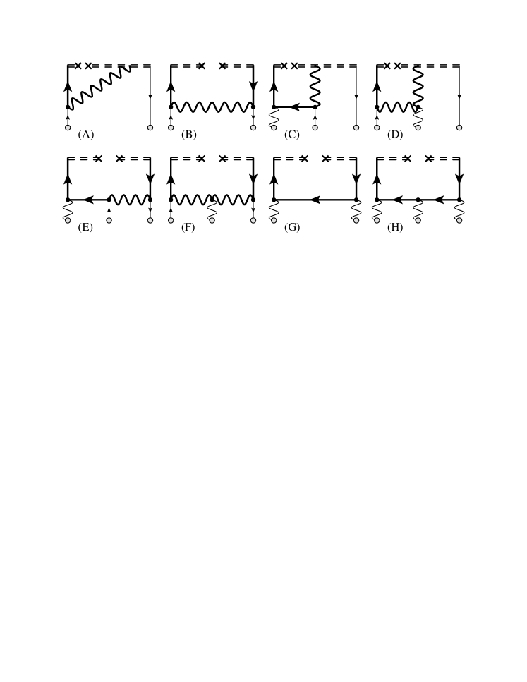
Figure 1: Diagrams contributing to the NLO effective operator at twist-two and twist-three level. The dashed lines show the half-infinite Wilson lines. The mirror diagrams to (A, C, D, E) should be added.

At the twist-three level one has to compute all diagrams of mass-dimension four. They are shown in fig.1. The diagrams with two external fields (A, B, G) have to be computed up to a single transverse-derivative contribution. These diagrams contain twist-two and twist-three parts, which can be identified using the QCD equations of motion. The diagrams with three external fields (C, D, E, F, H) contain only twist-three terms.

The diagrams have been evaluated in position space. It is the preferred representation for dealing with higher-twist operators, because the resulting expressions are much shorter in comparison to momentum space. Examples of diagram computations in this technique can be found in appendices of refs. Scimemi:2019gge ; Braun:2021aon ; Vladimirov:2021hdn . The final expressions in position space are presented in appendix B. The subsequent Fourier transformation to momentum space is laborious but straightforward.

As a by-product of the computations for diagrams A and B, we obtained the NLO matching coefficients for the TMDs $f_{1}$, $g_{1}$ and $h_{1}$. Our expressions coincides with well-known results Bacchetta:2013pqa ; Echevarria:2015uaa ; Gutierrez-Reyes:2017glx ; Buffing:2017mqm . This served as an intermediate check of our computation.

The computation is done for the bare operators and requires renormalization. Schematically the renormalization factor has the form

$$\Phi_{\text{renor.}}(\mu,\zeta)=Z^{-1}_{UV}(\mu,\zeta)R^{-1}(\zeta)\Phi_{\text{bare}}=Z^{-1}_{UV}(\mu,\zeta)R^{-1}(\zeta)\left(C_{\text{bare}}\otimes\phi_{\text{bare}}+...\right),$$ (42)

where in the last equality we inserted the bare small-$b$ expansion. Here, $Z_{UV}$ is the ultraviolet renormalization factor, and $R$ is the rapidity renormalization factor. We also renormalize the collinear distribution and obtain

$$\Phi_{\text{renor.}}(\mu,\zeta)=C_{\text{renor.}}(\mu,\zeta,\mu_{\text{OPE}})\otimes\phi_{\text{renor.}}(\mu_{\text{OPE}}),$$ (43)

where

$$C_{\text{renor.}}(\mu,\zeta,\mu_{\text{OPE}})=Z^{-1}_{UV}(\mu,\zeta)R^{-1}(\zeta)C_{\text{bare}}\otimes Z_{\phi}(\mu_{\text{OPE}}),$$ (44)

where $Z_{\phi}$ is the renormalization factor for the collinear distribution $\phi$. The function $C_{\text{renor.}}$ is finite.

To regularize divergences we use the combination of dimensional regularization and $\delta$-regularization (for rapidity divergences), which has been used in many TMD-related computations (see e.g. refs. Echevarria:2016scs ; Echevarria:2012js ; Buffing:2017mqm ). Collecting expressions for the LO renormalization factors Aybat:2011zv ; Echevarria:2015byo , we derive the following pocket formula for the renormalization of the NLO coefficient functions

$$C^{\text{NLO}}_{\text{renorm}} = \mu^{2\epsilon}e^{\epsilon\gamma_{E}}C_{\text{bare}}^{\text{NLO}}+\Big{[}\mu^{2\epsilon}e^{\epsilon\gamma_{E}}2\left(\frac{-b^{2}}{4}\right)^{\epsilon}C_{F}\Gamma(-\epsilon)\left(\mathbf{L}_{b}-\mathbf{l}_{\zeta}+2\ln\left(\frac{\delta^{+}}{p^{+}}\right)-\psi(-\epsilon)-\gamma_{E}\right)$$ (45)

$$-C_{F}\left(\frac{2}{\epsilon^{2}}+\frac{3+2\mathbf{l}_{\zeta}}{\epsilon}\right)-\frac{a_{s}}{\epsilon}\mathbb{H}\otimes\Big{]}C^{\text{LO}},$$

where the factors $\mu^{2\epsilon}e^{\epsilon\gamma_{E}}$ are the usual factors of the $\overline{\text{MS}}$-scheme, $\delta^{+}$ is the parameter of the $\delta$-regularization, $\epsilon$ is the parameter of the dimensional regularization ($d=4-2\epsilon$), and $\mathbb{H}$ is the LO evolution kernel for the corresponding collinear distribution. The cancellation of divergences in this combination is a very sensitive check of the computation.

3.3 Treatment of $\gamma_{5}$

The $\gamma^{5}$ matrix requires an additional treatment in dimensional regularization. In our computation we use the “Larin+”-scheme introduced in ref. Gutierrez-Reyes:2017glx . This is based on the four-dimensional identity

$$\gamma^{+}\gamma^{5}=\frac{i}{2!}\epsilon_{T}^{\mu\nu}\gamma^{+}\gamma_{\mu}\gamma_{\nu}.$$ (46)

The anti-symmetric tensor $\epsilon_{T}^{\mu\nu}$ is generalized to an arbitrary number of dimensions by means of the identity

$$\epsilon_{T}^{\mu_{1}\mu_{2}}\epsilon_{T}^{\nu_{1}\nu_{2}}=g_{T}^{\mu_{1}\nu_{1}}g_{T}^{\mu_{2}\nu_{2}}-g_{T}^{\mu_{1}\nu_{2}}g_{T}^{\mu_{2}\nu_{1}}.$$ (47)

This generalization is different from the ordinary Larin-scheme Larin:1993tq . The “Larin+”-scheme is preferable to the Larin-scheme, because it preserves the TMD-twist of an operator Gutierrez-Reyes:2017glx ; Rodini:2022wki , and consequently, the structure of its divergences.

The generalization of the $\gamma^{5}$ matrix to $d$-dimensions could also involve a multiplication by scheme-dependent factor $Z_{5}$. However, there is no necessity to introduce such factor for the TMD operators, because their renormalization is independent on the $\Gamma$-structure (as long as it preserves the TMD-twist). The factor $Z_{5}$ in the “Larin+”-scheme has been computed in ref. Gutierrez-Reyes:2017glx demanding the equality between helicity and unpolarized coefficient functions,

$$Z_{5}\otimes C_{q\leftarrow q}^{[\Gamma=\gamma^{+}\gamma^{5}]}=C_{q\leftarrow q}^{[\Gamma=\gamma^{+}]}.$$ (48)

Unfortunately, up to now, no accurate generalization of this scheme to the twist-three case exists.

In this work, we use the following procedure, which allows us to (partially) by-pass the problems associated with the definition of $\gamma^{5}$. First of all, we note that the problem exists only for the worm-gear-T function $g_{1T}$. For the chiral-odd operators with $\Gamma=i\sigma^{\alpha+}\gamma^{5}$, the $\gamma^{5}$-factor is illusory since $i\sigma^{\alpha+}\gamma^{5}=-\epsilon_{T}^{\alpha\beta}\sigma_{\beta+}$. The twist-two part of the function $g_{1T}$ can be computed using the standard definition. For the twist-three part of $g_{1T}$, we distinguish quark and gluon contributions. For the pure quark contributions we use an anti-commuting $\gamma^{5}$ (which is equivalent to implementing condition (48)). For the gluon contributions (diagrams G and H) we compute the trace using (46) and (47).

The result of this procedure (at NLO for the coefficient function) is equivalent to an $\overline{\text{MS}}$ twist-two computation. The deviations arrears at term suppressed by $\epsilon$ and at NNLO. It is straightforward to proof that the current scheme is equivalent at NLO to the ’t Hooft-Veltman-Breitenlohner-Maison tHooft:1972tcz ; Breitenlohner:1977hr scheme.

3.4 Twist-decomposition of the $F_{\mu+}D_{\alpha}F_{\nu+}$ operator

The diagrams A, B, and G result in two-point operators of generic twist-three. Such operators must be rewritten in terms of definite-twist-2 and -3 operators, which can be accomplished by using Dirac algebra and equations of motion.

For the diagrams A and B, these operators have the form $\bar{q}(zn)[zn,0]\Gamma_{T}q(0)$ where $\Gamma\in\{\gamma^{\mu},\gamma^{\mu}\gamma^{5},\sigma^{\mu\nu}\}$ (with $\mu$ and $\nu$ being transverse indices), and $\bar{q}(zn)[zn,0]\Gamma_{+}D_{\mu}q(0)$. The decomposition of such operators can be found in the literature, e.g. in refs. Balitsky:1987bk ; Scimemi:2018mmi ; Moos:2020wvd . A typical relation has the form

$$\langle p,S|\bar{q}(zn)[zn,0]\gamma^{\mu}\gamma^{5}q(0)|p,S\rangle = 2s_{T}^{\mu}M\int_{-1}^{1}dxe^{ix\zeta}g_{T}(x)$$

$$= 2s_{T}^{\mu}M\Big{(}\int_{0}^{1}d\alpha\widehat{g_{1}}(\zeta)+2\zeta^{2}\int_{0}^{1}d\alpha\int_{0}^{\bar{\alpha}}d\beta\beta\widehat{S}^{+}(\bar{\alpha}\zeta,\beta\zeta,0)\Big{)},$$

where $\zeta=zp_{+}$, $\bar{\alpha}=1-\alpha$, and $\widehat{g_{1}}$ and $\widehat{S}_{+}$ are Fourier transformations of the corresponding collinear distributions (92, 93). The first term in eqn. (3.4) gives the celebrated Wandzura-Wilczek relation Wandzura:1977qf .

For the diagram G the operator is $\mathbb{O}^{\mu\alpha\nu}(z)$ which comes from the expansion in $b$ of the leading-twist gluon TMD operator

$$\mathbb{O}^{\mu\alpha\nu}(z)=F^{\mu+}(zn+b)[zn,\pm\infty n]\overset{\leftarrow}{D}\phantom{\,}^{\alpha}[\pm\infty n,0]F^{\nu+}(0)$$ (50)

where all indices are transverse and the sign $\pm$ depends on the process. We have not found the decomposition of his operator in the literature and, therefore, perform it here.

To derive the decomposition, we have used the technique based on the spinor-helicity formalism developed in ref. Moos:2020wvd . This formalism yields in a natural way the result written as Fourier transformation of the momentum space representation. The operator $\mathbb{O}^{\mu\alpha\nu}$ has twist-two and twist-three parts

$$\mathbb{O}^{\mu\alpha\nu}(z)=[\mathbb{O}^{\mu\alpha\nu}(z)]_{\text{tw2}}+[\mathbb{O}^{\mu\alpha\nu}(z)]_{\text{tw3}}.$$ (51)

For the twist-two part we found

$$\langle p,S|\left[\mathbb{O}^{\mu\alpha\nu}(z)\right]_{\text{tw2}}|p,S\rangle = \frac{\epsilon_{T}^{\mu\nu}s_{T}^{\alpha}M}{2(1-\epsilon)(1-2\epsilon)}\text{FDF}^{\text{tw2}}(z)$$ (52)

$$= \frac{\epsilon_{T}^{\mu\nu}s_{T}^{\alpha}M}{2(1-\epsilon)(1-2\epsilon)}\int_{0}^{1}d\alpha\int_{-\infty}^{\infty}dye^{iy\alpha p^{+}z}(\alpha p^{+}y)^{2}\Delta f_{g}(y),$$ (53)

where $\Delta f_{g}$ is the gluon-helicity distribution (21). The twist-three term contains three tensor structures,

$$\langle p,S|\left[\mathbb{O}^{\mu\alpha\nu}(z)\right]_{\text{tw3}}|p,S\rangle = t_{2}^{\mu\alpha\nu}M\ \text{FDF}^{\text{tw3}}_{2}(z)+t_{4}^{\mu\alpha\nu}M\ \text{FDF}^{\text{tw3}}_{4}(z)+t_{6}^{\mu\alpha\nu}M\ \text{FDF}^{\text{tw3}}_{6}(z),$$ (54)

where

$$\text{FDF}^{\text{tw3}}_{2}(z) =\mp ip_{+}^{2}\pi\int_{-1}^{1}dyF^{+}_{2}(-y,0,y)e^{iyp_{+}z},$$

$$\text{FDF}^{\text{tw3}}_{4}(z) =\mp ip_{+}^{2}\pi\int_{-1}^{1}dyF^{+}_{4}(-y,0,y)e^{iyp_{+}z},$$

$$\text{FDF}^{\text{tw3}}_{6}(z) =p_{+}^{2}\int[dx]g^{+}(x_{1},x_{2},x_{3})\int_{0}^{1}du\left(\frac{3x_{1}+2x_{3}}{x_{2}^{2}}u^{2}e^{-iux_{1}p^{+}z}+\frac{x_{3}}{x_{2}^{2}}u^{2}e^{iux_{3}p^{+}z}\right)$$

$$+p_{+}^{2}\sum_{q}\int[dx]2T_{q}(x_{1},x_{2},x_{3})\int_{0}^{1}duu^{2}e^{-ip_{+}zux_{2}},$$

with $g^{+}=(2F_{2}^{+}+F_{4}^{+}+F_{6}^{+})$. The tensors $t_{i}^{\mu\nu\rho}$ and functions $F_{2,4,6}$ are defined in eqns.(31, 32, 33). The last term in $\text{FDF}^{\text{tw3}}_{6}$ is a consequence of the QCD equations of motion, and gives the singlet-quark contribution. (Note the sum over all active flavors.) The signs $\mp$ depend on the defining process, and are “-”(“+”) for SIDIS (Drell-Yan).

4 Results

In this section, we present the results for Sivers, Boer-Mulders and worm-gear TMDs in the small-$b$ regime at NLO. The expression for the Sivers function has been computed in ref. Scimemi:2019gge . In this paper, we have re-evaluated it as cross-check and present it here for completeness. The intermediate results of our computation, which could be interesting for theoretical investigations, are presented in appendix B.

In the formulas presented below we employ the notation for the logarithms defined in eqn.(13). The bar-variables are $\bar{\alpha}=1-\alpha$, $\bar{y}=1-y$, etc. The color factors are $C_{F}=(N_{c}^{2}-1)/2N_{c}$, $C_{A}=N_{c}$. For simplicity of presentation we use the delta-function form of the Mellin convolution

$$\int_{-1}^{1}dy\int_{0}^{1}d\alpha\delta(x-\alpha y)f(\alpha,y)=\left\{\begin{array}[]{lc}\displaystyle\int_{x}^{1}\frac{dy}{y}f\left(\frac{x}{y},y\right),&x>0,\\ \displaystyle\int_{-x}^{1}\frac{dy}{y}f\left(\frac{-x}{y},-y\right),&x<0.\end{array}\right.$$ (57)

The “plus”-distribution is defined as usual

$$(f(\alpha))_{+}=f(\alpha)-\delta(\bar{\alpha})\int_{0}^{1}d\beta f(\beta).$$ (58)

For all distributions the NLO expression has the following general form

$$F(x,b;\mu,\zeta) = F^{(0)}(x)+a_{s}\Bigg{\{}C_{F}\left(-\mathbf{L}_{b}^{2}+2\mathbf{L}_{b}\mathbf{l}_{\zeta}+3\mathbf{L}_{b}-\frac{\pi^{2}}{6}\right)F^{(0)}(x)$$

$$-2\mathbf{L}_{b}\mathbb{H}\otimes F^{(0)}(x)+F^{(1)}(x)\Bigg{\}}+\mathcal{O}(a_{s}^{2},b^{2}),$$

where $F^{(0)}$ is the tree-level expression, $F^{(1)}(x)$ is the finite part of the coefficient function, and $\mathbb{H}\otimes F^{(0)}$ contains the evolution kernel for the corresponding distribution,

$$\mu^{2}\frac{dF^{(0)}(x)}{d\mu^{2}}=2a_{s}\mathbb{H}\otimes F^{(0)}(x).$$ (60)

The parts proportional to the logarithms follow from the evolution equations (11, 22, 35). In each case, we found agreement between our results and the known evolution equations, see appendix A.

For practical applications, it is convenient to use the so-called optimal TMDs Scimemi:2018xaf ; Scimemi:2017etj . They are defined at $\zeta=\zeta(b,\mu)$, where $\zeta(b,\mu)$ is a null-evolution curve that passes through the saddle point of $(\gamma_{F},\mathcal{D})$-field Scimemi:2018xaf . To receive the coefficient function for optimal TMDs at NLO, it is enough to set $\mathbf{l}_{\zeta}$ according to

$$-\mathbf{L}_{b}^{2}+2\mathbf{L}_{b}\mathbf{l}_{\zeta}+3\mathbf{L}_{b}=0.$$ (61)

Note, that the remaining dependence on $\mu$ is compensated by the evolution of collinear PDF, and thus the remaining $\mu$ is the scale of OPE $\mu_{\text{OPE}}$.

4.1 Sivers function $f_{1T}^{\perp}$

The NLO expression for the Sivers function reads

$$f_{1T,q}^{\perp}(x,b;\mu,\zeta) = \pm\pi T_{q}(-x,0,x)\pm\pi a_{s}\Big{\{}C_{F}\left(-\mathbf{L}_{b}^{2}+2\mathbf{L}_{b}\mathbf{l}_{\zeta}+3\mathbf{L}_{b}-\frac{\pi^{2}}{6}\right)T_{q}(-x,0,x)$$

$$-2\mathbf{L}_{b}\mathbb{H}\otimes T_{q}(-x,0,x)+\mathbf{\delta f}_{1T}^{\perp}(x)\Big{\}}+\mathcal{O}(a_{s}^{2},b^{2}).$$

The finite part is

$$\mathbf{\delta f}_{1T}^{\perp}(x) = \int_{-1}^{1}dy\int_{0}^{1}d\alpha\delta(x-\alpha y)\Big{[}$$

$$\left(C_{F}-\frac{C_{A}}{2}\right)2\bar{\alpha}T_{q}(-y,0,y)+\frac{3\alpha\bar{\alpha}}{2}\frac{G_{+}(-y,0,y)+G_{-}(-y,0,y)}{y}\Big{]}.$$

The action of the evolution kernel on the function $T(-x,0,x)$ is

$$\mathbb{H}\otimes T_{q}(-x,0,x)=\int_{-1}^{1}dy\int_{0}^{1}d\alpha\delta(x-\alpha y)\Bigg{\{}$$ (64)

$$\qquad\left(C_{F}-\frac{C_{A}}{2}\right)\Big{[}\left(\frac{1+\alpha^{2}}{1-\alpha}\right)_{+}T_{q}(-y,0,y)+(2\alpha-1)_{+}T_{q}(-x,y,x-y)-\Delta T_{q}(-x,y,x-y)\Big{]}$$

$$\qquad+\frac{C_{A}}{2}\Big{[}\left(\frac{1+\alpha}{1-\alpha}\right)_{+}T_{q}(-x,x-y,y)+\Delta T_{q}(-x,x-y,y)\Big{]}$$

$$\qquad+\frac{1-2\alpha\bar{\alpha}}{4}\frac{G_{+}(-y,0,y)+Y_{+}(-y,0,y)+G_{-}(-y,0,y)+Y_{-}(-y,0,y)}{y}\Bigg{\}},$$

The choice of the sign $\pm$ is related to the process. For the case of Drell-Yan definition the ”$+$” sign should be taken. For the case of SIDIS definition ”$-$” sign should be taken.

In the present form, the NLO matching for the Sivers function (4.1) has been first computed in ref. Scimemi:2019gge . The logarithmic part (64) has been derived in ref. Braun:2009mi . The quark and gluon contributions to the finite part (4.1) were derived earlier in Sun:2013hua and Dai:2014ala , respectively, performing fixed-order computations for the SSA cross-sections. The detailed comparison of (4.1) with earlier work is given in ref. Scimemi:2019gge . In this contribution we have reproduced the results of Scimemi:2019gge which served us as a check of our computation.

4.2 Worm-gear-T function $g_{1T}$

The expression for the worm-gear-T function is the most cumbersome in this work. It is convenient to split it into twist-two and twist-three contributions

$$g_{1T,q}(x,b;\mu,\zeta)=g_{1T,q}^{\text{tw2}}(x,b;\mu,\zeta)+g_{1T,q}^{\text{tw3}}(x,b;\mu,\zeta).$$ (65)

The twist-two part is convenient to present in the form

$$g_{1T,q}^{\text{tw2}}(x,b;\mu,\zeta) = x\int_{x}^{1}\frac{dy}{y}\Big{[}C_{1T,q\leftarrow q}^{\text{tw2}}\left(\frac{x}{y}\right)g_{1q}(y)+C_{1T,q\leftarrow g}^{\text{tw2}}\left(\frac{x}{y}\right)\Delta f_{g}(y)\Big{]},$$ (66)

where

$$C_{1T,q\leftarrow q}^{\text{tw2}}(x) = 1+a_{s}C_{F}\left[-\mathbf{L}_{b}^{2}+2\mathbf{L}_{b}\mathbf{l}_{\zeta}-2\mathbf{L}_{b}\left(-\bar{x}+2\ln\bar{x}-\ln x\right)-2\bar{x}-2\ln x-\frac{\pi^{2}}{6}\right]+\mathcal{O}(a_{s}^{2}),$$

$$C_{1T,q\leftarrow g}^{\text{tw2}}(x) = \frac{a_{s}}{2}\left[-2\mathbf{L}_{b}(2\bar{x}+\ln x)+2\bar{x}+\ln x\right]+\mathcal{O}(a_{s}^{2}).$$ (67)

These expressions can be used as the Wandzura-Wilczek approximation for the worm-gear-T function. The logarithmic part of eqn. (66) coincides with the one predicted by evolution equations for helicity distributions (see e.g. Moch:2014sna ).

The twist-three part is complicated. We split it into a number of terms

$$g_{1T,q}^{\text{tw3}}(x,b;\mu,\zeta)=g_{1T,q}^{(0),\text{tw3}}(x)+a_{s}\Big{\{}C_{F}\left(-\mathbf{L}_{b}^{2}+2\mathbf{L}_{b}\mathbf{l}_{\zeta}+3\mathbf{L}_{b}-\frac{\pi^{2}}{6}\right)g_{1T,q}^{(0),\text{tw3}}(x)$$ (68)

$$\qquad-2\mathbf{L}_{b}\left(\mathbb{H}_{NS}+\mathbb{H}_{G}+\sum_{q^{\prime}}\mathbb{H}^{q^{\prime}}_{S}\right)\otimes g_{1T,q}^{\perp,(0),\text{tw3}}(x)+\mathbf{\delta g}_{NS}(x)+\mathbf{\delta g}_{G}(x)\Big{\}}+\mathcal{O}(a_{s}^{2},b^{2}).$$

We emphasize that the singlet-quark contribution to the finite part vanishes.

At the tree-level

$$g_{1T,q}^{(0),\text{tw3}}(x)=2x\int[dy]\int_{0}^{1}d\alpha\delta(x-\alpha y_{3})\left(\frac{\Delta T_{q}(y_{1,2,3})}{y_{2}^{2}}+\frac{T_{q}(y_{1,2,3})-\Delta T_{q}(y_{1,2,3})}{2y_{2}y_{3}}\right),$$ (69)

where $(y_{i,j,k})$ is a shorthand notation for $(y_{i},y_{j},y_{k})$. In this form the expression (69) has been derived in ref. Scimemi:2018mmi . The same result (but in a different basis) has been also derived in ref. Kanazawa:2015ajw .

The finite parts for eqn.(68) are

$$\mathbf{\delta g}_{NS}(x) = 2\int[dy]\int_{0}^{1}d\alpha\Bigg{\{}\left(C_{F}-\frac{C_{A}}{2}\right)\left(-\frac{\bar{\alpha}}{y_{3}}T+\frac{\bar{\alpha}(1-2\alpha)}{y_{3}}\Delta T\right)\delta(x-\alpha y_{2})$$

$$\qquad+\delta(x-\alpha y_{3})\Bigg{[}\left(-C_{F}\frac{\alpha\ln\alpha}{y_{2}}+\left(C_{F}-\frac{C_{A}}{2}\right)\frac{\bar{\alpha}y_{3}}{y_{1}y_{2}}\right)T$$

$$\qquad+\left(C_{F}\frac{\alpha\ln\alpha(y_{2}-2y_{3})-2\bar{\alpha}y_{3}}{y_{2}^{2}}+\left(C_{F}-\frac{C_{A}}{2}\right)\left(\frac{\bar{\alpha}(1-2\alpha)y_{3}}{y_{1}y_{2}}+\frac{2\bar{\alpha}^{2}y_{3}}{y_{2}^{2}}\right)\right)\Delta T\Bigg{]}\Bigg{\}},$$

$$\mathbf{\delta g}_{G}(x) = \int[dy]\int_{0}^{1}d\alpha\delta(x-\alpha y_{3})\Bigg{\{}$$

$$\qquad\alpha(\ln\alpha-2\bar{\alpha})\left(\frac{G_{+}(y_{1,2,3})-4Y_{+}(y_{2,3,1})}{y_{2}y_{3}}+2\frac{Y_{+}(y_{2,3,1})-Y_{+}(y_{3,1,2})}{y_{2}^{2}}\right)$$

$$\qquad+\alpha\bar{\alpha}\left(8\frac{Y_{+}(y_{2,3,1})-Y_{+}(y_{3,1,2})}{y_{2}^{2}}-18\frac{Y_{+}(y_{2,3,1})}{y_{2}y_{3}}\right)$$

$$\qquad+\bar{\alpha}\left(1-\frac{3}{8}\alpha\right)\frac{-G_{+}(y_{1,2,3})+G_{-}(y_{1,2,3})+2Y_{+}(y_{1,2,3})+2Y_{-}(y_{1,2,3})}{y_{1}y_{2}}\Bigg{\}},$$

where we use the shortened notation $T=T_{q}(y_{1},y_{2},y_{3})$, $\Delta T=\Delta T_{q}(y_{1},y_{2},y_{3})$ for the quark-gluon-quark distributions. Notice that the singlet quark contribution (summed over flavors) does not appear in the finite part. The logarithmic parts are

$$\mathbb{H}_{NS}\otimes g_{1T,q}^{(0),\text{tw3}}(x) = \int[dy]\int_{0}^{1}d\alpha\Bigg{\{}\delta(x-\alpha y_{3})\Bigg{[}$$

$$2xC_{F}\Big{\{}\left(\frac{1}{2}+\alpha-\ln\alpha+2\ln\bar{\alpha}\right)\left(\frac{T-\Delta T}{2y_{2}y_{3}}+\frac{\Delta T}{y_{2}^{2}}\right)-\frac{\Delta T}{y_{2}^{2}}\Big{\}}$$

$$+\left(C_{F}-\frac{C_{A}}{2}\right)\left(\alpha\frac{(2-\alpha)T-(4-3\alpha)\Delta T}{y_{2}}-\bar{\alpha}\frac{T-(1-2\alpha)\Delta T}{y_{1}}\right)$$

$$+\frac{C_{A}}{2}\Big{\{}\left(\frac{\alpha\bar{\alpha}-2}{y_{2}}-\frac{1}{x+y_{1}}\right)\left(T-\Delta T-2y_{3}\frac{\Delta T}{y_{2}}\right)-2(1-2\alpha)y_{3}\frac{\Delta T}{y_{2}^{2}}\Big{\}}\Bigg{]}$$

$$+\delta(x-\alpha y_{2})\left(C_{F}-\frac{C_{A}}{2}\right)\left(-\alpha+\bar{\alpha}^{2}\frac{y_{2}}{y_{3}}\right)\frac{T+(1-2\alpha)\Delta T}{x+y_{1}}$$

$$+\delta(x-y_{2}-\alpha y_{3})\left(C_{F}-\frac{C_{A}}{2}\right)\frac{1}{y_{2}}\left[T+\left(1+2\frac{\alpha y_{3}}{y_{2}}\right)\Delta T\right]\Bigg{\}},$$

$$\mathbb{H}_{G}\otimes g_{1T,q}^{(0),\text{tw3}}(x) = -\int[dy]\int_{0}^{1}d\alpha\delta(x-\alpha y_{3})\Bigg{\{}\frac{\alpha\bar{\alpha}}{2}\frac{Y_{+}(y_{2,3,1})-Y_{+}(y_{3,1,2})}{y_{2}y_{3}}$$

$$\qquad+\alpha(2\bar{\alpha}+\ln\alpha)\left(\frac{G_{+}(y_{1,2,3})-2Y_{+}(y_{2,3,1})}{y_{2}y_{3}}+\frac{Y_{+}(y_{2,3,1})-Y_{+}(y_{3,1,2})}{y_{2}^{2}}\right)$$

$$\qquad+\frac{\bar{\alpha}}{4}\frac{G_{+}(y_{1,2,3})-G_{-}(y_{1,2,3})}{y_{1}y_{2}}-\frac{\bar{\alpha}(1-3\alpha)}{2}\frac{Y_{+}(y_{3,1,2})-Y_{-}(y_{3,1,2})}{y_{1}y_{2}}$$

$$\qquad+\frac{\bar{\alpha}(1-2\alpha)}{2}\frac{Y_{+}(y_{2,3,1})-Y_{+}(y_{3,1,2})-Y_{-}(y_{2,3,1})+Y_{-}(y_{3,1,2})}{y_{2}^{2}}\Bigg{\}},$$

$$\mathbb{H}^{q^{\prime}}_{S}\otimes g_{1T,q}^{\perp,(0),\text{tw3}}(x) = 2\int[dy]\int_{0}^{1}d\alpha\delta(x-\alpha y_{2})(\alpha\bar{\alpha}+\alpha\ln\alpha)\frac{T_{q^{\prime}}(y_{1},y_{2},y_{3})}{y_{2}},$$ (74)

where we use the shortened notation $T=T_{q}(y_{1},y_{2},y_{3})$, $\Delta T=\Delta T_{q}(y_{1},y_{2},y_{3})$ for the quark-gluon-quark distributions, and $(y_{i,j,k})=(y_{i},y_{j},y_{k})$ for three-gluon distributions. To simplify these expressions we have used the symmetry relations (27) and (34).

The logarithmic part coincides with the prediction given by the renormalization group equation Braun:2009mi ; Braun:2009vc (see appendix A). It provides a strong check of our computation. The comparison has been made in position space (see appendix B). The integrands of eqns. (4.2 – 74) are finite for $y_{i}\to 0$. Also, we observed the cancelation of various undesirable terms such as $\ln^{2}\alpha$ and $\ln\bar{\alpha}/\alpha$ that appear in the individual diagrams. Altogether, these observations provide extra confidence in the result.

4.3 Boer-Mulders function $h_{1}^{\perp}$

The Boer-Mulders function is in many aspects similar to the Sivers function, which is the consequence of their T-oddness. We have

$$h_{1,q}^{\perp}(x,b;\mu,\zeta) = \mp\pi E_{q}(-x,0,x)\mp\pi a_{s}\Big{\{}C_{F}\left(-\mathbf{L}_{b}^{2}+2\mathbf{L}_{b}\mathbf{l}_{\zeta}+3\mathbf{L}_{b}-\frac{\pi^{2}}{6}\right)E_{q}(-x,0,x)$$

$$-2\mathbf{L}_{b}\mathbb{H}\otimes E_{q}(-x,0,x)\Big{\}}+\mathcal{O}(a_{s}^{2},b^{2}).$$

where the $\mp$ identifies the process under consideration. For DY (SIDIS) the upper (lower) sign should be taken. For the Boer-Mulders function, we have found that the finite part (besides the $\pi^{2}/6$ contribution), exactly vanishes, i.e.:

$$\mathbf{\delta h}_{1,f}^{\perp}(x) = 0$$ (76)

For the evolution kernel, we have

$$\mathbb{H}\otimes E_{q}(-x,0,x)=-\frac{C_{F}}{2}E_{q}(-x,0,x)+\int_{0}^{1}d\alpha\int dy\delta(x-\alpha y)\Big{\{}$$ (77)

$$\qquad 2\left(C_{F}-\frac{C_{A}}{2}\right)\Big{[}\left(\frac{\alpha}{1-\alpha}\right)_{+}E_{q}(-y,0,y)-\bar{\alpha}E_{q}(-x,y,x-y)\Big{]}+C_{A}\frac{E_{q}(-x,x-y,y)}{(1-\alpha)_{+}}\Big{\}}.$$

In general the expression for the Boer-Mulders function has the simplest form among all TMD distributions that match twist-three operators. The expression for the evolution kernel agrees with the general kernel for the twist-three functions Braun:2009vc ; Braun:2021gvv , see also appendix A.

4.4 Worm-gear-L function $h_{1L}^{\perp}$

It is convenient to split the expression for the worm-gear-T function into twist-two and twist-three contributions

$$h_{1L,q}^{\perp}(x,b;\mu,\zeta)=h_{1L,q}^{\perp,\text{tw2}}(x,b;\mu,\zeta)+h_{1L,q}^{\perp,\text{tw3}}(x,b;\mu,\zeta).$$ (78)

The twist-two part can be written in the form

$$h_{1L,q}^{\perp,\text{tw2}}(x,b;\mu,\zeta) = -x^{2}\int_{x}^{1}\frac{dy}{y}C_{1L,q\leftarrow q}^{\perp,\text{tw2}}\left(\frac{x}{y}\right)h_{1}(y),$$ (79)

where

$$C_{1L,q\leftarrow q}^{\perp,\text{tw2}}(x) = 1+a_{s}C_{F}\left[-\mathbf{L}_{b}^{2}+2\mathbf{L}_{b}\mathbf{l}_{\zeta}-4\mathbf{L}_{b}\left(\ln x-\ln\bar{x}\right)-\frac{\pi^{2}}{6}\right]+\mathcal{O}(a_{s}^{2}),$$

These expressions can be used as the Wandzura-Wilczek-like approximation for the worm-gear-L function. The logarithmic part of eqn. (79) coincides with the one predicted by evolution equations for transversity distributions (see e.g. Vogelsang:1997ak ). The finite part contains only the trivial contribution $\pi^{2}/6$. The non-trivial part vanishes (see the diagram $\mathbf{B}$ in sec.B.3).

The twist-three part is

$$h_{1L,q}^{\perp,\text{tw3}}(x,b;\mu,\zeta) = h_{1L,q}^{\perp,(0),\text{tw3}}(x)+a_{s}\Big{\{}C_{F}\left(-\mathbf{L}_{b}^{2}+2\mathbf{L}_{b}\mathbf{l}_{\zeta}+3\mathbf{L}_{b}-\frac{\pi^{2}}{6}\right)h_{1L,q}^{\perp,(0),\text{tw3}}(x)$$

$$-2\mathbf{L}_{b}\mathbb{H}\otimes h_{1L,q}^{\perp,(0),\text{tw3}}(x)+\mathbf{\delta h}(x)\Big{\}}+\mathcal{O}(a_{s}^{2},b^{2}).$$

At tree-level it is

$$h_{1L,q}^{\perp,(0),\text{tw3}}(x)=-2x\int_{0}^{1}d\alpha\int[dy]\alpha\delta(x-\alpha y_{3})H_{q}(y_{1},y_{2},y_{3})\frac{y_{3}-y_{2}}{y_{2}^{2}y_{3}}.$$ (81)

This expression has been derived in refs. Scimemi:2018mmi ; Kanazawa:2015ajw . Note that the integral is finite for $y_{2}\to 0$, since $H(-y,0,y)=0$.

The finite and logarithmic parts of the twist-three expression are

$$\mathbf{\delta h}(x)=-4\int[dy]H_{q}(y_{1},y_{2},y_{3})\Bigg{\{}$$ (82)

$$\qquad\int_{0}^{1}d\alpha\Big{[}\left(C_{F}-\frac{C_{A}}{2}\right)\alpha\bar{\alpha}\left(\frac{\delta(x-\alpha y_{2})}{y_{3}}-\frac{\delta(x-\alpha y_{3})}{y_{1}}\right)+\frac{C_{A}}{2}\bar{\alpha}(\alpha y_{2}+\bar{\alpha}y_{3})\frac{\delta(x-\alpha y_{3})}{y_{2}^{2}}\Big{]}$$

$$\qquad+\int_{0}^{1}d\alpha\int_{0}^{1}d\beta\frac{\alpha}{x+y_{1}}\left(\frac{C_{A}}{2}\delta(x+\alpha y_{1}+\alpha\beta y_{2})-\left(C_{F}-\frac{C_{A}}{2}\right)\delta(x+\alpha y_{1}+\alpha\beta y_{3})\right)\Bigg{\}}.$$

$$\mathbb{H}\otimes h_{1L,q}^{\perp,(0),\text{tw3}}(x)=-2\int[dy]H_{q}(y_{1},y_{2},y_{3})\Bigg{\{}$$ (83)

$$\qquad\int_{0}^{1}d\alpha C_{F}\alpha x\left(\frac{3}{2}+2\ln\bar{\alpha}-2\ln\alpha\right)\frac{y_{3}-y_{2}}{y_{2}^{2}y_{3}}\delta(x-\alpha y_{3})$$

$$\qquad+\int_{0}^{1}d\alpha\int_{0}^{1}d\beta\frac{\alpha(y_{2}-x)}{y_{2}(x+y_{1})}\left(\frac{C_{A}}{2}\delta(x+\alpha y_{1}+\alpha\beta y_{2})-\left(C_{F}-\frac{C_{A}}{2}\right)\delta(x+\alpha y_{1}+\alpha\beta y_{3})\right)\Bigg{\}}.$$

The double-integrals in the last lines of these equations can be integrated over one of the variables, but the resulting expressions have a complicated form.

5 Conclusion

We have computed the leading small-$b$ asymptotics for Sivers ($f_{1T}^{\perp}$), Boer-Mulders ($h_{1}^{\perp}$) and worm-gear functions ($g_{1T}$ and $h_{1L}^{\perp}$) at NLO in perturbation theory. These functions are expressed in terms of twist-two and twist-three collinear distributions. The computation is performed using the well-established background-field method, which was also used for similar computations in refs. Scimemi:2019gge ; Braun:2021aon ; Braun:2021gvv . The result is presented both in position (appendix B) and momentum-fraction (section 4) space. The logarithmic parts of the obtained expressions agree with the predictions of the renormalization group equations. The result for the Sivers function coincides with the one computed in ref. Scimemi:2019gge .

With the results of this work the knowledge of small-$b$ expressions for TMDs of leading twist is complete at NLO (or even higher, see refs. Luo:2020epw ; Gutierrez-Reyes:2018iod ). The only distribution for which this is still missing is pretzelosity that has leading twist-four contributions at small-$b$ Moos:2020wvd . In the transverse momentum space the computed expressions corresponds to the large momentum asymptotic of TMDs.

The perturbative expansions for the Sivers and Boer-Mulders functions on one side and the worm-gear functions on the other side are drastically different, which is a consequence of the T-parity properties of these functions. So, the Sivers and Boer-Mulders at LO have the Qiu-Sterman form of quark-anti-quark correlators with a null-momentum gluon field Qiu:1991pp $T(-x,0,x)$ and $E(-x,0,x)$. The NLO expressions for these distributions contain only twist-three distributions and are relatively simple (in particular, the finite part of the Boer-Mulders function is trivial (76)). The global sign of the small-$b$ expression depends on the orientation of the gauge link.

In contrast, the worm-gear functions have involved forms. Already at LO, they are expressed by convolution integrals of twist-two and twist-three distributions, which lead to bulky NLO expressions. The expression for the worm-gear-T distribution is especially cumbersome, since it contains mixtures with a three-gluon correlator and a singlet-quark contribution. Unfortunately, we have not found any significant simplifications for these distributions. At the moment, the most practically important result for worm-gear functions is the part proportional to twist-two distributions, because it can be used as an approximation for these functions (Wandzura-Wilczek-like approximation). The goodness of such an approximation is difficult to establish at the moment. It remains, however, a useful one given the currently available data.

The derived NLO expressions are important for the phenomenology of TMDs and twist-three distributions. They provide the leading logarithmic terms, and thus allow to properly include QCD evolution effects in the data analysis. This will be definitely important for the next-generation of high-precision polarized experiments such as EIC AbdulKhalek:2021gbh .

Appendix A Evolution equations for twist-three collinear distributions

In this appendix, we collect the expressions for the LO evolution kernels of twist-three distributions $\widehat{F}$. The expressions are given in position space where they are more compact and which we used for the checks of our computations. We define

$$\widehat{F}(\zeta_{1},\zeta_{2},\zeta_{3})=\int[dx]e^{-i(\zeta_{1}x_{1}+\zeta_{2}x_{2}+\zeta_{3}x_{3})}F(x_{1},x_{2},x_{3}),$$ (84)

for $F\in\{S^{\pm},T,\Delta T,H,E,F_{2},F_{4},F_{6}\}$.

The evolution equations in position space have the form

$$\mu^{2}\frac{d}{d\mu^{2}}\widehat{F}(\zeta_{1},\zeta_{2},\zeta_{3})=2a_{s}[\mathbb{H}\otimes\widehat{F}](\zeta_{1},\zeta_{2},\zeta_{3}),$$ (85)

where $\mathbb{H}$ is an integral operator. The derivation and original expressions for the kernels can be found in refs. Balitsky:1987bk ; Braun:2009vc . The momentum space expressions are much longer. They can be found (in parts) in refs. Ji:2014eta ; Braun:2009mi ; Vladimirov:2021hdn .

The evolution kernel for the quark-gluon-quark chiral-even operators has three flavor contributions

$$[\mathbb{H}\otimes\widehat{F}_{q}]=[\mathbb{H}_{NS}\otimes\widehat{F}_{q}]+[\mathbb{H}_{G}\otimes\widehat{F}_{q}]+\sum_{q^{\prime}}[\mathbb{H}^{q^{\prime}}_{S}\otimes\widehat{F}_{q}],$$ (86)

where $q$ labels the flavor of the quark field, and we omit the arguments $(z_{1},z_{2},z_{3})$ in each term. The non-singlet part for the function $\widehat{S}^{+}$ reads

$$[\mathbb{H}_{NS}\otimes\widehat{S}^{+}](\zeta_{1},\zeta_{2},\zeta_{3})$$ (87)

$$\quad=\frac{C_{A}}{2}\int_{0}^{1}d\alpha\Big{[}\frac{\bar{\alpha}\widehat{S}^{+}(\zeta_{12}^{\alpha},\zeta_{2},\zeta_{3})+\bar{\alpha}\widehat{S}^{+}(\zeta_{1},\zeta_{2},\zeta_{32}^{\alpha})+\bar{\alpha}^{2}\widehat{S}^{+}(\zeta_{1},\zeta_{21}^{\alpha},\zeta_{3})+\bar{\alpha}^{2}\widehat{S}^{+}(\zeta_{1},\zeta_{23}^{\alpha},\zeta_{3})}{(\alpha)_{+}}$$

$$\qquad+2\int_{0}^{\bar{\alpha}}d\beta\bar{\beta}\widehat{S}^{+}(\zeta_{12}^{\alpha},\zeta_{21}^{\beta},\zeta_{3})\Big{]}$$

$$\qquad+\left(C_{F}-\frac{C_{A}}{2}\right)\int_{0}^{1}d\alpha\Big{[}\frac{\bar{\alpha}\widehat{S}^{+}(\zeta_{13}^{\alpha},\zeta_{2},\zeta_{3})+\bar{\alpha}\widehat{S}^{+}(\zeta_{1},\zeta_{2},\zeta_{31}^{\alpha})}{(\alpha)_{+}}-\bar{\alpha}\widehat{S}^{+}(\zeta_{1},\zeta_{32}^{\alpha},\zeta_{3})$$

$$\qquad+\int_{0}^{\bar{\alpha}}d\beta\widehat{S}^{+}(\zeta_{13}^{\alpha},\zeta_{2},\zeta_{31}^{\beta})-2\int_{\bar{\alpha}}^{1}d\beta\bar{\beta}\widehat{S}^{+}(\zeta_{12}^{\alpha},\zeta_{21}^{\beta},\zeta_{3})\Big{]}+\frac{3}{2}C_{F}\widehat{S}^{+}(\zeta_{1},\zeta_{2},\zeta_{3}),$$

where

$$\bar{\alpha}=1-\alpha,\qquad\zeta_{ij}=\zeta_{i}\bar{\alpha}+\zeta_{j}\alpha.$$

The gluon mixing (also for the $\widehat{S}^{+}$ function) is

$$[\mathbb{H}_{G}\otimes\widehat{S}^{+}](z_{1},z_{2},z_{3})$$ (88)

$$\quad=-i(\zeta_{1}-\zeta_{3})\Big{[}\int_{0}^{1}d\alpha\int_{0}^{\bar{\alpha}}d\beta(1-\alpha-\beta+2\alpha\beta)(g^{+}+g^{-})+\int_{0}^{1}d\alpha\int_{\bar{\alpha}}^{1}d\beta\bar{\alpha}\bar{\beta}(-g^{+}+g^{-})\Big{]},$$

where

$$g^{\pm}=2\widehat{F}_{2}^{\pm}(\zeta_{13}^{\alpha},\zeta_{2},\zeta_{31}^{\beta})+\widehat{F}_{4}^{\pm}(\zeta_{13}^{\alpha},\zeta_{2},\zeta_{31}^{\beta})+\widehat{F}_{6}^{\pm}(\zeta_{13}^{\alpha},\zeta_{2},\zeta_{31}^{\beta}),$$ (89)

with $\widehat{F}_{1,2,3}$ being defined in eqn.(32, 33). Finally, the mixture with the quark-gluon-quark operators (of all active flavors including the original one) is

$$[\mathbb{H}_{S}^{q}\otimes\widehat{S}^{+}](\zeta_{1},\zeta_{2},\zeta_{3})=\int_{0}^{1}d\alpha\,\alpha\bar{\alpha}\widehat{S}^{+}(\zeta_{13}^{\alpha},\zeta_{2},\zeta_{13}^{\alpha}).$$ (90)

This contribution appears via the QCD equation of motion in the diagrams with external “bad” components of gluon fields (see e.g. Ji:2001bm ).

The evolution kernel of the chiral-odd functions is

$$[\mathbb{H}\otimes\widehat{F}](\zeta_{1},\zeta_{2},\zeta_{3})$$ (91)

$$\quad=\frac{C_{A}}{2}\int_{0}^{1}d\alpha\Big{[}\frac{\bar{\alpha}\widehat{F}(\zeta_{12}^{\alpha},\zeta_{2},\zeta_{3})+\bar{\alpha}\widehat{F}(\zeta_{1},\zeta_{2},\zeta_{32}^{\alpha})+\bar{\alpha}^{2}\widehat{F}(\zeta_{1},\zeta_{21}^{\alpha},\zeta_{3})+\bar{\alpha}^{2}\widehat{F}(\zeta_{1},\zeta_{23}^{\alpha},\zeta_{3})}{(\alpha)_{+}}$$

$$\qquad+2\int_{0}^{\bar{\alpha}}d\beta\bar{\beta}\left(\widehat{F}(\zeta_{12}^{\alpha},\zeta_{21}^{\beta},\zeta_{3})+\widehat{F}(\zeta_{1},\zeta_{23}^{\beta},\zeta_{32}^{\alpha})\right)\Big{]}$$

$$\qquad+\left(C_{F}-\frac{C_{A}}{2}\right)\int_{0}^{1}d\alpha\Big{[}\frac{\bar{\alpha}\widehat{F}(\zeta_{13}^{\alpha},\zeta_{2},\zeta_{3})+\bar{\alpha}\widehat{F}(\zeta_{1},\zeta_{2},\zeta_{31}^{\alpha})}{(\alpha)_{+}}$$

$$\qquad-2\int_{\bar{\alpha}}^{1}d\beta\bar{\beta}\left(\widehat{F}(\zeta_{12}^{\alpha},\zeta_{21}^{\beta},\zeta_{3})+\widehat{F}(\zeta_{1},\zeta_{23}^{\beta},\zeta_{31}^{\alpha})\right)\Big{]}+\frac{3}{2}C_{F}\widehat{F}(\zeta_{1},\zeta_{2},\zeta_{3}),$$

where $\widehat{F}$ stands for $\widehat{H}$ or $\widehat{E}$. Note, that the equation can be simplified for each case using (anti)symmetry of the functions $\widehat{E}(\widehat{H})$.

Appendix B Intermediate expressions in position space

In this appendix we provide the full set of expressions in position space obtained by evaluating the diagrams with the background field method. For the twist-two distributions, $F\in\{f_{1},g_{1},h_{1},f_{g},\Delta f_{g}\}$ we define

$$\widehat{F}(\zeta)=\int_{-1}^{1}dxe^{ix\zeta}F(x).$$ (92)

For the twist-three distributions $F\in\{S^{\pm},T,\Delta T,H,E,G,Y\}$ we define

$$\widehat{F}(\zeta_{1},\zeta_{2},\zeta_{3})=\int[dx]e^{-i(\zeta_{1}x_{1}+\zeta_{2}x_{2}+\zeta_{3}x_{3})}F(x_{1},x_{2},x_{3}),$$ (93)

being $[dx]=dx_{1}dx_{2}dx_{3}\delta(x_{1}+x_{2}+x_{3})$. In position space the collinear distributions satisfy translation invariance

$$\widehat{F}(\zeta_{1}+\tau,\zeta_{2}+\tau,\zeta_{3}+\tau)=\widehat{F}(\zeta_{1},\zeta_{2},\zeta_{3}).$$ (94)

In the following formulas, we have used this relation together with the symmetry relations to simplify expressions.

In the following we use the notation $[d\alpha d\beta d\gamma]$ to denote the integral over the simplex of Feynman variables, i.e.

$$\int[d\alpha d\beta d\gamma]=\int_{0}^{1}d\alpha\int_{0}^{1}d\beta\int_{0}^{1}d\gamma\delta(1-\alpha-\beta-\gamma)$$ (95)

We present the results for both SIDIS- and DY-like TMDs. For this reason, it is convenient to introduce $L$ as

$$L=\begin{cases}+\infty&\text{SIDIS-like process},\\ -\infty&\text{DY-like process}.\end{cases}$$ (96)

For all diagrams we show the contribution to a particular TMD. For example, for $g_{1T}$ we extract the coefficient of $(b\cdot s_{T})$, and divide it by $iM$.

B.1 Worm-gear-T function $g_{1T}$

Diagrams A and B are most conveniently written in terms of the tree level expressions for the matching of the worm-gear function $g_{1T}$ and for the function $g_{T}$. In position space they are:

$$\begin{split}\widehat{g}_{1T}^{tree}(\zeta)&=\frac{1}{i\zeta}\left(\widehat{g}_{1}(\zeta)+\int_{0}^{1}d\beta\widehat{g}_{1}(\beta\zeta)\right)+i\left(\int_{L}^{0}d\tau-\int_{0}^{-L}d\tau\right)\widehat{S}^{+}(\zeta,\tau,0)\\ &+i\zeta\int[d\alpha d\beta d\gamma]\left(2\beta\widehat{S}^{+}(\bar{\alpha}\zeta,\beta\zeta)+2\widehat{S}^{+}(\zeta,\beta\zeta,0)\right),\\ \widehat{g}_{T}(\zeta)&=\int_{0}^{1}d\alpha\widehat{g}_{1}(\alpha\zeta)+2\zeta^{2}\int[d\alpha d\beta d\gamma]\beta\widehat{S}^{+}(\bar{\alpha}\zeta,\beta\zeta,0).\end{split}$$ (97)

We use the distributions $S^{+},T,\Delta T$ to present the results. These are linked by the following relations

$$\widehat{T}(\zeta_{1},\zeta_{2},\zeta_{3}) = \widehat{T}(-\zeta_{3},-\zeta_{2},-\zeta_{1}),\quad\widehat{\Delta T}(\zeta_{1},\zeta_{2},\zeta_{3})=-\widehat{\Delta T}(-\zeta_{3},-\zeta_{2},-\zeta_{1}),$$ (98)

$$2\widehat{S}^{\pm}(\zeta_{1},\zeta_{2},\zeta_{3}) = -\widehat{T}(\zeta_{1},\zeta_{2},\zeta_{3})\pm\widehat{\Delta T}(\zeta_{1},\zeta_{2},\zeta_{3}),\quad\widehat{S}^{+}(\zeta_{1},\zeta_{2},\zeta_{3})=\widehat{S}^{-}(-\zeta_{3},-\zeta_{2},-\zeta_{1})$$ (99)

On a diagram by diagram basis, we have for $g_{1T}$:

$$\bm{A+A^{*}} = 2a_{s}C_{F}B^{\epsilon}\Gamma(-\epsilon)\int_{0}^{1}d\alpha\left(\frac{2\alpha}{\bar{\alpha}}\right)_{+}\alpha\widehat{g}_{1T}^{tree}(\alpha\zeta)-2\delta(\bar{\alpha})(1+\lambda_{\delta})\widehat{g}_{1T}^{tree}(\alpha\zeta),$$ (100)

$$\bm{B} = 2a_{s}(1-\epsilon)\Gamma(-\epsilon)C_{F}B^{\epsilon}\int_{0}^{1}d\alpha\ 2\alpha\bar{\alpha}\hat{g}^{tree}_{1T}(\alpha\zeta)+(1-2\alpha)\frac{\widehat{g}_{T}(\alpha\zeta)}{i\zeta},$$ (101)

$$\bm{C+C^{*}} = ia_{s}\left(C_{F}-\frac{C_{A}}{2}\right)\Gamma(-\epsilon)B^{\epsilon}\int[d\alpha d\beta d\gamma]\left[\int_{L}^{0}d\tau-\int_{0}^{-L}d\tau\right]$$

$$\times\Bigg{\{}2\frac{\beta}{\bar{\beta}}\widehat{\Delta T}\left(\beta\zeta;\tau-\alpha\zeta;0\right)$$

$$-\left(2\frac{\alpha}{\bar{\beta}}-1\right)\widehat{\Delta T}\left(\zeta_{\tau\zeta}^{\beta};\alpha(\tau-\zeta);0\right)+\widehat{T}\left(\zeta_{\tau\zeta}^{\beta};\alpha(\tau-\zeta);0\right)\Bigg{\}},$$

$$\bm{D+D^{*}} = -ia_{s}\frac{C_{A}}{2}\Gamma(-\epsilon)B^{\epsilon}\left(\int_{L}^{0}d\tau-\int_{0}^{-L}d\tau\right)\int[d\alpha d\beta d\gamma]$$

$$\times\Bigg{[}\left(1+2\frac{\alpha}{\beta}\right)\widehat{\Delta T}(\zeta_{\zeta\tau}^{\beta},\alpha(\zeta-\tau),0)+\widehat{T}(\zeta_{\zeta\tau}^{\beta},\alpha(\zeta-\tau),0)$$

$$+2\frac{\bar{\beta}}{\beta}\widehat{\Delta T}(\bar{\beta}\zeta,\tau+\alpha\zeta,0)\Bigg{]},$$

$$\bm{E+E^{*}} = -ia_{s}\Gamma(-\epsilon)B^{\epsilon}\left(C_{F}-\frac{C_{A}}{2}\right)\int[d\alpha d\beta d\gamma]\left(\int_{L}^{0}d\tau-\int_{0}^{-L}d\tau\right)$$

$$\times\Bigg{[}(1-\epsilon)(1-4\gamma)\widehat{\Delta T}\left(\alpha\zeta;\tau-\beta\zeta;0\right)-(1+\epsilon)\widehat{T}\left(\alpha\zeta;\tau-\beta\zeta;0\right)\Bigg{]}\Bigg{]},$$

$$\bm{F} = -2ia_{s}\frac{C_{A}}{2}\Gamma(-\epsilon)(1-\epsilon)B^{\epsilon}\int[d\alpha d\beta d\gamma]\beta\left(\int_{L}^{0}d\tau-\int_{0}^{-L}d\tau\right)\widehat{\Delta T}(\bar{\beta}\zeta,\tau+\alpha\zeta,0),$$ (105)

$$\bm{G} = ia_{s}\Gamma(-\epsilon)B^{\epsilon}\int_{0}^{1}d\alpha\Bigg{[}\frac{\alpha}{2}\left(2\alpha-1-2\bar{\alpha}\frac{\epsilon}{1-\epsilon}\right)\left(\int_{L}^{0}d\tau-\int_{0}^{-L}d\tau\right)\text{FDF}^{\text{tw2}}(\tau+\alpha\zeta)$$

$$+(1-2\epsilon)\alpha(2\alpha-1-2\epsilon\bar{\alpha})\left(\int_{L}^{0}d\tau-\int_{0}^{-L}d\tau\right)\text{FDF}^{\text{tw3}}_{6}(\tau+\alpha\zeta)$$

$$-i(1-2\epsilon)^{2}\frac{\bar{\alpha}\alpha}{2}\left(\int_{L}^{0}d\tau-\int_{0}^{-L}d\tau\right)\left(\int_{L}^{0}d\sigma-\int_{0}^{-L}d\sigma\right)F_{6}(\sigma+\alpha\zeta,\tau,0)$$

$$-2(1-2\epsilon)\left(\int_{L}^{0}d\tau-\int_{0}^{-L}d\tau\right)\alpha\bar{\alpha}\widehat{T}(0,\tau+\alpha\zeta,0)\Bigg{]}.$$

For diagram H, we present the result using light-cone gauge for the background fields, which allows us to write

$$A^{\mu}(z)=-\int_{L}^{0}d\tau F^{\mu+}(\tau+z).$$ (107)

For more details on this relation, we refer to Ref. Vladimirov:2021hdn . Also, to present the result in a compact form, we define $\partial_{1,2,3}$ as derivatives acting only on $A^{\mu}$, $A^{\nu}$ and $A^{\sigma}$, respectively. We obtain:

$$\bm{H} =\frac{ga_{s}\Gamma(-\epsilon)B^{\epsilon}}{4i(b\cdot s_{T})M}\int[d\alpha d\beta d\gamma d\rho](d^{ABC}+if^{ABC})\braket{P}{A^{\mu}_{A}(\beta\zeta)A^{\nu}_{B}((\beta+\gamma)\zeta)A^{\sigma}_{C}(\bar{\alpha}\zeta)}{P}$$ (108)

$$+ib^{\sigma}(\partial_{1}^{+}-\partial_{3}^{+})\epsilon_{T}^{\mu\nu}(\gamma\zeta\partial_{1}^{+}-\rho\zeta\partial_{3}^{+}-1)$$

$$+ib^{\nu}\epsilon_{T}^{\mu\sigma}\left(\gamma(2\gamma-1)\zeta(\partial_{1}^{+})^{2}+\rho(2\rho-1)\zeta(\partial_{3}^{+})^{2}-8\gamma\partial_{1}^{+}+8\rho\partial_{3}^{+}-\partial_{1}^{+}\partial_{3}^{+}\zeta(4\gamma\rho-\gamma-\rho)+4\partial_{1}^{+}+\partial_{2}^{+}\right)$$

$$-ib^{\mu}\epsilon_{T}^{\nu\sigma}\left(\gamma(2\gamma-1)\zeta(\partial_{1}^{+})^{2}+\rho(2\rho-1)\zeta(\partial_{3}^{+})^{2}-8\gamma\partial_{1}^{+}+8\rho\partial_{3}^{+}-\partial_{1}^{+}\partial_{3}^{+}\zeta(4\gamma\rho-\gamma-\rho)-4\partial_{3}^{+}-\partial_{2}^{+}\right)$$

$$+i\epsilon_{T}^{\mu\rho}b_{\rho}\left(g^{\nu\sigma}\left(\rho\zeta\partial_{2}^{+}\partial_{3}^{+}-\gamma\zeta\partial_{1}^{+}\partial_{2}^{+}+\partial_{2}^{+}-2\partial_{3}^{+}\right)+4\epsilon\partial_{1}^{+}\frac{b^{\nu}b^{\sigma}}{b^{2}}\right)$$

$$+i\epsilon_{T}^{\nu\rho}b_{\rho}\left(g^{\mu\sigma}\left(\rho\zeta\partial_{2}^{+}\partial_{3}^{+}-\gamma\zeta\partial_{1}^{+}\partial_{2}^{+}+\partial_{2}^{+}-2\partial_{1}^{+}\right)+4\epsilon\partial_{3}^{+}\frac{b^{\mu}b^{\sigma}}{b^{2}}\right)$$

$$+i\epsilon_{T}^{\sigma\rho}b_{\rho}\left(g^{\mu\nu}\left(\gamma\zeta\partial_{1}^{+}\partial_{2}^{+}-\rho\zeta\partial_{2}^{+}\partial_{3}^{+}-\partial_{2}^{+}\right)+4\epsilon\partial_{2}^{+}\frac{b^{\mu}b^{\nu}}{b^{2}}\right).$$ (109)

The factor $i(b\cdot s_{T})M$ comes from the definition of $g_{1T}(\zeta,b)$. Expanding the result for diagram $\bm{H}$ and writing it in terms of distributions is most conveniently done using directly the momentum space representation.

B.2 Boer-Mulders function $h_{1}^{\perp}$

The Boer-Mulders function is similar to the Sivers function. It has only a twist-3 contribution. Specifically we have

$$\widehat{h}_{1}^{\perp,tree}(\zeta)=-\frac{1}{2}\int_{L}^{-L}d\tau\widehat{E}(\zeta,\tau,0).$$ (110)

The function $E(\zeta_{1},\zeta_{2},\zeta_{3})$ obeys the symmetry relation

$$\widehat{E}(\zeta_{1},\zeta_{2},\zeta_{3})=\widehat{E}(-\zeta_{3},-\zeta_{2},-\zeta_{1})$$ (111)

In this expression, it is trivial to see that, passing from SIDIS-like processes to DY-like processes, the function changes sign.

For the individual diagrams, we have

$$\bm{A+A^{*}} =2a_{s}C_{F}B^{\epsilon}\Gamma(-\epsilon)\int_{0}^{1}d\alpha\left(\frac{2\alpha}{\bar{\alpha}}\right)_{+}\alpha\widehat{h}_{1}^{\perp,tree}(\alpha\zeta)-2\delta(\bar{\alpha})(1+\lambda_{\delta})\widehat{h}_{1}^{\perp,tree}(\alpha\zeta),$$

$$\bm{B} =4a_{s}C_{F}\Gamma(1-\epsilon)B^{\epsilon}\int d\alpha\alpha\bar{\alpha}\widehat{h}_{1}^{\perp}(\alpha\zeta),$$

$$\bm{C+C^{*}} =2a_{s}\Gamma(-\epsilon)\left(C_{F}-\frac{C_{A}}{2}\right)B^{\epsilon}\int_{0}^{1}d\alpha\int_{L}^{-L}d\tau\left(\alpha\widehat{E}(\tau,\zeta_{\zeta\tau}^{\alpha},0)-\alpha\widehat{E}(\alpha\zeta,\tau,0)\right),$$

$$\bm{D+D^{*}} =2a_{s}\Gamma(-\epsilon)B^{\epsilon}\frac{C_{A}}{2}\int[d\alpha d\beta d\gamma]\int_{L}^{-L}d\tau\left[-\bar{\beta}\widehat{E}(\zeta_{\zeta\tau}^{\alpha},\zeta_{\tau\zeta}^{\beta},0)-\frac{\bar{\alpha}\bar{\beta}}{\alpha}\widehat{E}(\zeta_{\zeta\tau}^{\alpha},\zeta_{\tau\zeta}^{\beta},0)-\widehat{E}(\bar{\alpha}\zeta,\zeta_{\tau\zeta}^{\beta},0)\right],$$

$$\bm{E+E^{*}} =2a_{s}\left(C_{F}-\frac{C_{A}}{2}\right)\Gamma(1-\epsilon)B^{\epsilon}\int_{0}^{1}d\alpha\ \alpha\bar{\alpha}\int_{L}^{-L}d\tau\widehat{E}(\alpha\zeta;\tau;0),$$

$$\bm{F} =2a_{s}\frac{C_{A}}{2}\Gamma(1-\epsilon)B^{\epsilon}\int_{0}^{1}d\alpha\ \alpha\bar{\alpha}\int_{L}^{-L}d\tau\widehat{E}(\alpha\zeta,\tau,0).$$ (112)

It is straightforward to convince oneself that the sum $\bm{B+E+E^{*}+F}$ vanishes identically. Therefore, the only non-zero contribution is to the pole part.

B.3 Worm-gear-L function $h_{1L}^{\perp}$

The worm-gear function $h_{1L}^{\perp}$ behaves similar to the worm-gear function $g_{1T}$, but has no gluon-contributions. Specifically, one has both twist-three and twist-three tree-level matching:

$$\widehat{h}_{1L}^{\perp,tree}(\zeta) =\frac{1}{i\zeta}\left(2\int_{0}^{1}d\alpha\alpha\widehat{h}_{1}(\alpha\zeta)-\widehat{h}_{1}(\zeta)\right)+i\zeta\int_{0}^{1}d\beta\beta\widehat{H}(\zeta,\beta\zeta,0)$$

$$-i\zeta\int[d\alpha d\beta d\gamma]2\beta^{2}\widehat{H}(\bar{\alpha}\zeta,\beta\zeta,0)-\frac{i}{2}\left(\int_{L}^{0}d\tau-\int_{0}^{-L}d\tau\right)\widehat{H}(\zeta,\tau,0),$$

$$\widehat{h}_{L}(\zeta) =2\int_{0}^{1}d\alpha\alpha\widehat{h}_{1}(\alpha\zeta)+2\zeta^{2}\int[d\alpha d\beta d\gamma]\beta^{2}\widehat{H}(\bar{\alpha}\zeta,\beta\zeta,0),$$ (113)

where the function $\widehat{H}$ obeys the symmetry relation

$$\widehat{H}(\zeta_{1},\zeta_{2},\zeta_{3})=-\widehat{H}(-\zeta_{3},-\zeta_{2},-\zeta_{1}).$$ (114)

For individual diagrams, we find:

$$\bm{A+A^{*}} =2a_{s}C_{F}B^{\epsilon}\Gamma(-\epsilon)\int_{0}^{1}d\alpha\left(\frac{2\alpha}{\bar{\alpha}}\right)_{+}\alpha\widehat{h}_{1L}^{\perp,tree}(\alpha\zeta)-2\delta(\bar{\alpha})(1+\lambda_{\delta})\widehat{h}_{1L}^{\perp,tree}(\alpha\zeta),$$

$$\bm{B} =-2a_{s}C_{F}\Gamma(1-\epsilon)B^{\epsilon}\int d\alpha\ 2\alpha\bar{\alpha}\widehat{h}_{1L}^{\perp,tree}(\alpha\zeta)-(1-2\alpha)\frac{\widehat{h}_{L}(\alpha\zeta)}{i\zeta},$$

$$\bm{C+C^{*}} =-ia_{s}\Gamma(-\epsilon)\left(C_{F}-\frac{C_{A}}{2}\right)B^{\epsilon}p^{+}\int[d\alpha d\beta d\gamma]\left[\int_{L}^{0}d\tau-\int_{0}^{-L}d\tau\right]$$

$$\times\left[2\frac{\beta}{\bar{\beta}}\widehat{H}(\beta\zeta,\tau-\alpha\zeta,0)+2\frac{\gamma}{\bar{\beta}}\widehat{H}(\zeta_{\tau\zeta}^{\beta},\alpha(\tau-\zeta),0)-2\epsilon\widehat{H}(\zeta_{\tau\zeta}^{\beta},\alpha(\tau-\zeta),0)\right],$$

$$\bm{D+D^{*}} =ia_{s}\frac{C_{A}}{2}B^{\epsilon}\Gamma(-\epsilon)\int[d\alpha d\beta d\gamma]\left(\int_{L}^{0}d\tau-\int_{0}^{-L}d\tau\right)\Bigg{\{}$$

$$\left(\frac{2\bar{\alpha}}{\beta}-2\epsilon\right)\widehat{H}(\zeta_{\zeta\tau}^{\beta},\gamma(\zeta-\tau),0)+\frac{2\bar{\beta}}{\beta}\widehat{H}(\bar{\beta}\zeta,\tau+\alpha\zeta,0)\Bigg{\}},$$

$$\bm{E+E^{*}} =2ia_{s}\left(C_{F}-\frac{C_{A}}{2}\right)\Gamma(1-\epsilon)B^{\epsilon}$$

$$\times\int[d\alpha d\beta d\gamma]\left(\int_{L}^{0}d\tau-\int_{0}^{-L}d\tau\right)(2\gamma-1+\epsilon)\widehat{H}(\alpha\zeta,\tau-\beta\zeta,0),$$

$$\bm{F} =-2i\Gamma(1-\epsilon)a_{s}\frac{C_{A}}{2}B^{\epsilon}\int[d\alpha d\beta d\gamma]\ \beta\left(\int_{L}^{0}d\tau-\int_{0}^{-L}d\tau\right)\widehat{H}(\bar{\beta}\zeta,\tau+\alpha\zeta,0).$$ (116)

It is interesting to observe that after substitution of (113) the twist-two part of the diagram $\mathbf{B}$ vanishes. It leads to a trivial finite part for the twist-two contribution.

References

• (1) P.J. Mulders and R.D. Tangerman, The Complete tree level result up to order 1/Q for polarized deep inelastic leptoproduction, Nucl. Phys. B 461 (1996) 197 [hep-ph/9510301].
• (2) D. Boer and P.J. Mulders, Time reversal odd distribution functions in leptoproduction, Phys. Rev. D 57 (1998) 5780 [hep-ph/9711485].
• (3) D. Boer, R. Jakob and P.J. Mulders, Angular dependences in electroweak semiinclusive leptoproduction, Nucl. Phys. B 564 (2000) 471 [hep-ph/9907504].
• (4) I. Scimemi and A. Vladimirov, Non-perturbative structure of semi-inclusive deep-inelastic and Drell-Yan scattering at small transverse momentum, JHEP 06 (2020) 137 [1912.06532].
• (5) A. Bacchetta, V. Bertone, C. Bissolotti, G. Bozzi, M. Cerutti, F. Piacenza et al., Unpolarized Transverse Momentum Distributions from a global fit of Drell-Yan and Semi-Inclusive Deep-Inelastic Scattering data, 2206.07598.
• (6) J. Collins, Foundations of perturbative QCD, vol. 32, Cambridge University Press (11, 2013).
• (7) V. Moos and A. Vladimirov, Calculation of transverse momentum dependent distributions beyond the leading power, JHEP 12 (2020) 145 [2008.01744].
• (8) M.A. Ebert, B. Mistlberger and G. Vita, TMD Fragmentation Functions at N3LO, JHEP 07 (2021) 121 [2012.07853].
• (9) M.-x. Luo, T.-Z. Yang, H.X. Zhu and Y.J. Zhu, Unpolarized quark and gluon TMD PDFs and FFs at N3LO, JHEP 06 (2021) 115 [2012.03256].
• (10) D. Gutierrez-Reyes, I. Scimemi and A. Vladimirov, Transverse momentum dependent transversely polarized distributions at next-to-next-to-leading-order, JHEP 07 (2018) 172 [1805.07243].
• (11) D. Gutierrez-Reyes, S. Leal-Gomez, I. Scimemi and A. Vladimirov, Linearly polarized gluons at next-to-next-to leading order and the Higgs transverse momentum distribution, JHEP 11 (2019) 121 [1907.03780].
• (12) D. Gutiérrez-Reyes, I. Scimemi and A.A. Vladimirov, Twist-2 matching of transverse momentum dependent distributions, Phys. Lett. B 769 (2017) 84 [1702.06558].
• (13) M.G.A. Buffing, M. Diehl and T. Kasemets, Transverse momentum in double parton scattering: factorisation, evolution and matching, JHEP 01 (2018) 044 [1708.03528].
• (14) A. Bacchetta and A. Prokudin, Evolution of the helicity and transversity Transverse-Momentum-Dependent parton distributions, Nucl. Phys. B 875 (2013) 536 [1303.2129].
• (15) K. Kanazawa, Y. Koike, A. Metz, D. Pitonyak and M. Schlegel, Operator Constraints for Twist-3 Functions and Lorentz Invariance Properties of Twist-3 Observables, Phys. Rev. D 93 (2016) 054024 [1512.07233].
• (16) I. Scimemi and A. Vladimirov, Matching of transverse momentum dependent distributions at twist-3, Eur. Phys. J. C 78 (2018) 802 [1804.08148].
• (17) S. Meissner, A. Metz and K. Goeke, Relations between generalized and transverse momentum dependent parton distributions, Phys. Rev. D 76 (2007) 034002 [hep-ph/0703176].
• (18) D. Boer, P.J. Mulders and F. Pijlman, Universality of T odd effects in single spin and azimuthal asymmetries, Nucl. Phys. B 667 (2003) 201 [hep-ph/0303034].
• (19) X. Ji, J.-W. Qiu, W. Vogelsang and F. Yuan, A Unified picture for single transverse-spin asymmetries in hard processes, Phys. Rev. Lett. 97 (2006) 082002 [hep-ph/0602239].
• (20) J. Zhou, F. Yuan and Z.-T. Liang, Transverse momentum dependent quark distributions and polarized Drell-Yan processes, Phys. Rev. D 81 (2010) 054008 [0909.2238].
• (21) L.-Y. Dai, Z.-B. Kang, A. Prokudin and I. Vitev, Next-to-leading order transverse momentum-weighted Sivers asymmetry in semi-inclusive deep inelastic scattering: the role of the three-gluon correlator, Phys. Rev. D 92 (2015) 114024 [1409.5851].
• (22) I. Scimemi, A. Tarasov and A. Vladimirov, Collinear matching for Sivers function at next-to-leading order, JHEP 05 (2019) 125 [1901.04519].
• (23) A. Bacchetta, F. Delcarro, C. Pisano, M. Radici and A. Signori, Extraction of partonic transverse momentum distributions from semi-inclusive deep-inelastic scattering, Drell-Yan and Z-boson production, JHEP 06 (2017) 081 [1703.10157].
• (24) I. Scimemi and A. Vladimirov, Analysis of vector boson production within TMD factorization, Eur. Phys. J. C 78 (2018) 89 [1706.01473].
• (25) Jefferson Lab Angular Momentum collaboration, Origin of single transverse-spin asymmetries in high-energy collisions, Phys. Rev. D 102 (2020) 054002 [2002.08384].
• (26) M.G. Echevarria, Z.-B. Kang and J. Terry, Global analysis of the Sivers functions at NLO+NNLL in QCD, JHEP 01 (2021) 126 [2009.10710].
• (27) M. Bury, F. Hautmann, S. Leal-Gomez, I. Scimemi, A. Vladimirov and P. Zurita, PDF bias and flavor dependence in TMD distributions, 2201.07114.
• (28) S. Bhattacharya, Z.-B. Kang, A. Metz, G. Penn and D. Pitonyak, First global QCD analysis of the TMD g1T from semi-inclusive DIS data, Phys. Rev. D 105 (2022) 034007 [2110.10253].
• (29) M. Bury, A. Prokudin and A. Vladimirov, Extraction of the Sivers function from SIDIS, Drell-Yan, and $W^{\pm}/Z$ boson production data with TMD evolution, JHEP 05 (2021) 151 [2103.03270].
• (30) M. Bury, A. Prokudin and A. Vladimirov, Extraction of the Sivers Function from SIDIS, Drell-Yan, and $W^{\pm}/Z$ Data at Next-to-Next-to-Next-to Leading Order, Phys. Rev. Lett. 126 (2021) 112002 [2012.05135].
• (31) J.C. Collins and D.E. Soper, Back-To-Back Jets in QCD, Nucl. Phys. B 193 (1981) 381.
• (32) P. Sun and F. Yuan, Transverse momentum dependent evolution: Matching semi-inclusive deep inelastic scattering processes to Drell-Yan and W/Z boson production, Phys. Rev. D 88 (2013) 114012 [1308.5003].
• (33) I.I. Balitsky and V.M. Braun, Evolution Equations for QCD String Operators, Nucl. Phys. B 311 (1989) 541.
• (34) V.M. Braun, Y. Ji and A. Vladimirov, QCD factorization for twist-three axial-vector parton quasidistributions, JHEP 05 (2021) 086 [2103.12105].
• (35) V.M. Braun, Y. Ji and A. Vladimirov, QCD factorization for chiral-odd parton quasi- and pseudo-distributions, JHEP 10 (2021) 087 [2108.03065].
• (36) A. Vladimirov, V. Moos and I. Scimemi, Transverse momentum dependent operator expansion at next-to-leading power, 2109.09771.
• (37) S. Rodini and A. Vladimirov, Definition and evolution of transverse momentum dependent distribution of twist-three, 2204.03856.
• (38) J.C. Collins, Leading twist single transverse-spin asymmetries: Drell-Yan and deep inelastic scattering, Phys. Lett. B 536 (2002) 43 [hep-ph/0204004].
• (39) A. Vladimirov, Structure of rapidity divergences in multi-parton scattering soft factors, JHEP 04 (2018) 045 [1707.07606].
• (40) S.M. Aybat and T.C. Rogers, TMD Parton Distribution and Fragmentation Functions with QCD Evolution, Phys. Rev. D 83 (2011) 114042 [1101.5057].
• (41) D. Boer, L. Gamberg, B. Musch and A. Prokudin, Bessel-Weighted Asymmetries in Semi Inclusive Deep Inelastic Scattering, JHEP 10 (2011) 021 [1107.5294].
• (42) R.L. Jaffe, Spin, twist and hadron structure in deep inelastic processes, in Ettore Majorana International School of Nucleon Structure: 1st Course: The Spin Structure of the Nucleon, pp. 42–129, 1, 1996 [hep-ph/9602236].
• (43) Z.-B. Kang and J.-W. Qiu, Evolution of twist-3 multi-parton correlation functions relevant to single transverse-spin asymmetry, Phys. Rev. D 79 (2009) 016003 [0811.3101].
• (44) D. Boer, P.J. Mulders and O.V. Teryaev, Single spin asymmetries from a gluonic background in the Drell-Yan process, Phys. Rev. D 57 (1998) 3057 [hep-ph/9710223].
• (45) Y. Kanazawa and Y. Koike, Chiral odd contribution to single transverse spin asymmetry in hadronic pion production, Phys. Lett. B 478 (2000) 121 [hep-ph/0001021].
• (46) H. Eguchi, Y. Koike and K. Tanaka, Twist-3 Formalism for Single Transverse Spin Asymmetry Reexamined: Semi-Inclusive Deep Inelastic Scattering, Nucl. Phys. B 763 (2007) 198 [hep-ph/0610314].
• (47) V.M. Braun, G.P. Korchemsky and A.N. Manashov, Gluon contribution to the structure function g(2)(x, Q**2), Nucl. Phys. B 597 (2001) 370 [hep-ph/0010128].
• (48) H. Beppu, Y. Koike, K. Tanaka and S. Yoshida, Contribution of Twist-3 Multi-Gluon Correlation Functions to Single Spin Asymmetry in Semi-Inclusive Deep Inelastic Scattering, Phys. Rev. D 82 (2010) 054005 [1007.2034].
• (49) M.J. Dugan and B. Grinstein, On the vanishing of evanescent operators, Phys. Lett. B 256 (1991) 239.
• (50) R.L. Jaffe, Parton Distribution Functions for Twist Four, Nucl. Phys. B 229 (1983) 205.
• (51) V.M. Braun, A.N. Manashov and J. Rohrwild, Renormalization of Twist-Four Operators in QCD, Nucl. Phys. B 826 (2010) 235 [0908.1684].
• (52) Y. Ji and A.V. Belitsky, Renormalization of twist-four operators in light-cone gauge, Nucl. Phys. B 894 (2015) 161 [1405.2828].
• (53) M.G. Echevarria, T. Kasemets, P.J. Mulders and C. Pisano, QCD evolution of (un)polarized gluon TMDPDFs and the Higgs $q_{T}$-distribution, JHEP 07 (2015) 158 [1502.05354].
• (54) Z.-B. Kang, B.-W. Xiao and F. Yuan, QCD Resummation for Single Spin Asymmetries, Phys. Rev. Lett. 107 (2011) 152002 [1106.0266].
• (55) M.G. Echevarria, I. Scimemi and A. Vladimirov, Unpolarized Transverse Momentum Dependent Parton Distribution and Fragmentation Functions at next-to-next-to-leading order, JHEP 09 (2016) 004 [1604.07869].
• (56) L.F. Abbott, Introduction to the Background Field Method, Acta Phys. Polon. B 13 (1982) 33.
• (57) M.G. Echevarría, A. Idilbi and I. Scimemi, Soft and Collinear Factorization and Transverse Momentum Dependent Parton Distribution Functions, Phys. Lett. B 726 (2013) 795 [1211.1947].
• (58) M.G. Echevarria, I. Scimemi and A. Vladimirov, Universal transverse momentum dependent soft function at NNLO, Phys. Rev. D 93 (2016) 054004 [1511.05590].
• (59) S.A. Larin, The Renormalization of the axial anomaly in dimensional regularization, Phys. Lett. B 303 (1993) 113 [hep-ph/9302240].
• (60) G. ’t Hooft and M.J.G. Veltman, Regularization and Renormalization of Gauge Fields, Nucl. Phys. B 44 (1972) 189.
• (61) P. Breitenlohner and D. Maison, Dimensional Renormalization and the Action Principle, Commun. Math. Phys. 52 (1977) 11.
• (62) S. Wandzura and F. Wilczek, Sum Rules for Spin Dependent Electroproduction: Test of Relativistic Constituent Quarks, Phys. Lett. B 72 (1977) 195.
• (63) I. Scimemi and A. Vladimirov, Systematic analysis of double-scale evolution, JHEP 08 (2018) 003 [1803.11089].
• (64) V.M. Braun, A.N. Manashov and B. Pirnay, Scale dependence of twist-three contributions to single spin asymmetries, Phys. Rev. D 80 (2009) 114002 [0909.3410].
• (65) S. Moch, J.A.M. Vermaseren and A. Vogt, The Three-Loop Splitting Functions in QCD: The Helicity-Dependent Case, Nucl. Phys. B 889 (2014) 351 [1409.5131].
• (66) W. Vogelsang, Next-to-leading order evolution of transversity distributions and Soffer’s inequality, Phys. Rev. D 57 (1998) 1886 [hep-ph/9706511].
• (67) J.-w. Qiu and G.F. Sterman, Single transverse spin asymmetries, Phys. Rev. Lett. 67 (1991) 2264.
• (68) R. Abdul Khalek et al., Science Requirements and Detector Concepts for the Electron-Ion Collider: EIC Yellow Report, 2103.05419.
• (69) X.-D. Ji and J. Osborne, An Analysis of the next-to-leading order corrections to the g(T) = g(1) + g(s)) scaling function, Nucl. Phys. B 608 (2001) 235 [hep-ph/0102026].