LiteDepth: Digging into Fast and Accurate
Depth Estimation on Mobile Devices

Abstract

Monocular depth estimation is an essential task in the computer vision community. While tremendous successful methods have obtained excellent results, most of them are computationally expensive and not applicable for real-time on-device inference. In this paper, we aim to address more practical applications of monocular depth estimation, where the solution should consider not only the precision but also the inference time on mobile devices. To this end, we first develop an end-to-end learning-based model with a tiny weight size (1.4MB) and a short inference time (27FPS on Raspberry Pi 4). Then, we propose a simple yet effective data augmentation strategy, called R² crop, to boost the model performance. Moreover, we observe that the simple lightweight model trained with only one single loss term will suffer from performance bottleneck. To alleviate this issue, we adopt multiple loss terms to provide sufficient constraints during the training stage. Furthermore, with a simple dynamic re-weight strategy, we can avoid the time-consuming hyper-parameter choice of loss terms. Finally, we adopt the structure-aware distillation to further improve the model performance. Notably, our solution named LiteDepth ranks 2^nd in the MAI&AIM2022 Monocular Depth Estimation Challenge, with a si-RMSE of 0.311, an RMSE of 3.79, and the inference time is 37$ms$ tested on the Raspberry Pi 4. Notably, we provide the fastest solution to the challenge. Codes and models will be released at https://github.com/zhyever/LiteDepth.

1 Introduction

Monocular depth estimation plays a vital role in the computer vision community, where a wide spread of various depth-depended tasks related to autonomous driving [6, 36, 8, 31, 7, 40, 22, 39], virtual reality [3, 11], and scene understanding [46, 37, 13, 35] provide strong demand for fast and accurate monocular depth estimation methods that are applicable to portable low-power hardware. Therefore, research along the line of accelerating depth estimation while reducing quality sacrifice on mobile devices has drawn increasing attention [15, 38].

As a classic ill-posed problem, estimating accurate depth from a single image is challenging. However, with the fast development of deep learning techniques, neural network demonstrates groundbreaking improvement with plausible depth estimation results [9, 20, 5, 42, 24, 25]. While engaging results have been presented, most of these state-of-the-art (SoTA) models are only optimized for high fidelity results while not taking into account computational efficiency and mobile-related constraints. The requirements of powerful high-end GPUs and consuming gigabytes of RAM lead to a dilemma when developing these models on resource-constrained mobile hardware [15, 1, 2].

In this paper, we aim to address the more practical application problem of monocular depth estimation on mobile devices, where the solution should consider not only the precision but also the inference time [15]. We first investigate a suitable network design. Typically, the depth estimation network follows a UNet paradigm [32] consisting of an encoder and a decoder with skip connections. Regarding the encoder, we choose a variant version of MobileNet-v3 [14] as a trade-off between performance and inference time, where we drop out the last convolution layer to speed up inference and reduce the model size. Moreover, we observe that the commonly used image normalization pre-process on input images is also time-consuming (19$ms$ on Raspberry Pi 4). To solve this issue, we propose to merge the normalization into the first convolution layer in a post-process manner so that the redundant overhead can be eliminated without bells and whistles. Following [15], we adopt the fast downsampling strategy, which could quickly downsample the resolution of input images from 480 $\times$ 640 to 4 $\times$ 6. A light decoder is introduced to recover the spatial details, consisting of a few convolutional layers and upsampling layers.

After determining the model structure, we propose several effective training strategies to boost the fidelity of the lightweight model. (1) We adopt an effective augmentation strategy called R² crop. It not only adopts crop patches on images with Random locations but also Randomly changes the size of crop patches. This strategy increases the diversity of the scenes and effectively avoids overfitting the training set. (2) We introduce a multiple-loss training strategy to provide sufficient supervision during the training stage, where we propose a gradience loss that can handle invalid holes in training samples and adopt the other three loss terms proposed in previous works. Moreover, we install a dynamic re-weighting strategy that can avoid the time-consuming weight selection of loss terms. (3) We highlight that our work focuses on the model training strategies, unlike previous solutions that adopt variant distillation methods [15, 38]. However, model distillation can also be an effective way to boost the model fidelity without any overhead. Therefore, we adopt the structure-aware distillation [27] in a fine-tuning manner.

We evaluate our method on Mobile AI (MAI2022) dataset, and the results demonstrate that each strategy can improve the accuracy of the lightweight network. With a short inference time (37$ms$ per image) on Raspberry Pi 4 and a lightweight model design (totally 1.4MB), our solution named MobileDepth achieves results of 0.311 si-RMSE and ranks second in the MAI&AIM 2022 Monocular Depth Estimation Challenge [18].

In summary, our main contributions are:

• We design a lightweight depth estimation model that achieves fast inference on mobile hardware, where an image normalization merging strategy is proposed to reduce the redundant overhead.

• We adopt an effective augmentation strategy called R² crop that is adopted at random locations on images with a randomly changed size of patches.

• We design a gradience loss that can handle invalid holes in training samples and propose to apply multiple-loss items to provide sufficient supervision during the training stage.

• We evaluate our method on MAI2022 dataset and rank second place in the MAI&AIM2022 Monocular Depth Estimation Challenge [18].

Table 1: Ranking results in the MAI&AIM2022 Monocular Depth Estimation Challenge, which are evaluated on the online test server. We highlight our results in bold.

Rank Username  si-RMSE    RMSE    log₁₀     REL  Runtime   Score 1 TCL 0.277 3.47 0.110 0.299 46$ms$ 297.79 2 Zhenyu Li 0.311 3.79 0.124 0.342 37$ms$ 232.04 3 ChaoMI 0.299 3.89 0.134 0.380 54$ms$ 187.77 4 parkzyzhang 0.303 3.80 12.189 0.301 68$ms$ 141.07 5 RocheL 0.329 4.06 0.137 0.366 65$ms$ 102.07 6 mvc 0.349 4.46 0.140 0.340 139$ms$ 36.07 7 Byung Hyun Lee 0.338 6.73 0.332 0.507 142$ms$ 41.58

2 Related Work

Monocular depth estimation is an ill-posed problem [9]. Lack of cues, scale ambiguities, translucent or reflective materials all leads to ambiguous cases where appearance cannot infer the spatial construction [24]. With the rapid development of deep learning, the neural network has dominated the primary workhorse to provide reasonable depth maps from a single RGB input [43, 20, 5, 24, 25].

Eigen et al. [9] first groundbreakingly propose a multi-scale deep network, consisting of a global network and a local network to predict the coarse depth and refine predictions, respectively. Subsequent works focus on various points to boost depth estimation, for instance, problem formulation [10, 5, 25], network architecture [20, 24, 19], supervision design [4, 43, 30], interpretable method [44], pre-training strategy [23, 29], unsupervised training [12, 45], etc. Though achieving engaging fidelity, these methods neglect the limitation of resource-constrained hardware and can be hard to develop on portable devices or embedded systems.

Notably, there are also some methods that take the inference time and model complexity into account, which makes them applicable on mobile devices [15]. FastDepth [41] deploys a real-time depth estimation method on embedded systems by designing an efficient model architecture and a pruning strategy to further reduce the model complexity. In our paper, we follow FastDepth [41] to choose MobileNet-v3 [14] as our encoder and design an even more lightweight decoder (only consisting of four convolution layers) to achieve a trade-off between fidelity and inference speed.

3 Method

In this section, we first present our network design in Sec. 3.1, where tons of details should be considered to achieve the best trade-off between fidelity and inference speed. Then, we introduce our proposed R² Crop in Sec. 3.2 and Multiple Loss Training strategy in Sec. 3.3. Subsequently, we illustrate the installation of the structure-aware Distillation strategy in Sec. 3.4.

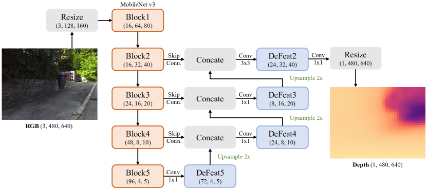
Figure 1: Illustration of our proposed network architecture that follows the prevalent Unet [32] design consisting of a MobileNet-V3 [14] encoder and a lightweight decoder with skip connections.

3.1 Network Design

As shown in Fig. 1, our proposed network consists of an encoder and a lightweight decoder with skip connections. We sequentially introduce each component and design detail.

Encoder plays a crucial role in extracting features from input images for depth estimation. To achieve a trade-off between fidelity and inference speed, we choose MobileNet-v3 [14] as our encoder. It is worth noticing that MobileNet contains a dimension-increasing layer (1$\times$1 convolution with an input dimension of 96 and output dimension of 960) to facilitate training for a classification task. We remove this layer to improve the inference speed and reduce the number of model parameters. Following [15], we adopt the Fast Downsampling Strategy in which a resize layer is inserted at the beginning of the encoder to resize the high-resolution input image from 480 × 640 to 128 × 160. As a result, the encoder can quickly downsample the resolution of feature maps, significantly shorten the inference time. Typically, input images are normalized to align with the pre-training setting. We discern the vanilla image normalization is time-consuming (19$ms$ of the image normalization v.s. 37$ms$ of the whole model) on the target device (i.e., Raspberry Pi 4). Therefore, we propose to merge the image normalization into the first convolution layer in a post-process manner so that we can avoid the redundant overhead without bells and whistles. Consider the image normalization and the first convolution layer:

$$I_{n}=\frac{I_{r}-m}{s},$$ (1)

$$f=W*I_{n}+b,$$ (2)

where $I_{n}$ and $I_{r}\in\mathbb{R}^{3\times H\times W}$ are normalized and raw input images. $m\in\mathbb{R}^{3}$ and $s\in\mathbb{R}^{3}$ are the mean and standard deviation used in the image normalization. $f\in\mathbb{R}^{C\times H_{f}\times W_{f}}$ is the output feature map with $C$ channels of the first convolution in our network. $W\in\mathbb{R}^{3\times C\times k^{2}}$ and $b\in\mathbb{R}^{C}$ are the trained weight and bias of the first $k\times k$ convolution. $*$ denotes the convolution operation. Given a trained model with parameters $W$ and $b$ of the first convolution, we update the them based on the mean and standard deviation used in the image normalization during the training stage:

$$W^{\prime}=\frac{W}{s},$$ (3)

$$b_{i}^{\prime}=b_{i}-\sum\limits_{d}^{3}\left(\frac{m_{d}}{s_{d}}\times\sum\limits_{j}^{k\times k}W_{dij}\right),~{}i\in(1,2,...,C),$$ (4)

$$b^{\prime}=\mathbf{Concat}([b_{1}^{\prime},b_{2}^{\prime},...,b_{C}^{\prime}]),$$ (5)

where the $W^{\prime}$ and $b^{\prime}$ are the updated weight and bias of the first $k\times k$ convolution. $\mathbf{Concat}$ is the element-wise concatenation. $d$ is the index of RGB dimension. Consequently, we discard the image normalization and apply the first convolution directly on input images as:

$$f=W^{\prime}*I_{r}+b^{\prime}.$$ (6)

As a result, the trained network can directly recieve the raw input images without the time-consuming image normalization.

Decoder is adopted to recover the spatial details by fusing the multi-level deep and shallow features. Unlike previous works [41, 15, 38] that utilize the symmetrical encoder and decoder, we drop out the last decoder layer to further accelerate the model inference. Hence, the resolution of outputs is 4$\times$ downsampled (i.e., 32$\times$64). At each decoding stage, we apply a simple feature fusion module to aggregate the decoded and skip-connected features, which consists of a concatenation operation and a convolution layer (with ReLU as the activation function). To achieve the best trade-off between fidelity and speed, we utilize the 1$\times$1 and 3$\times$3 convolution for deep and shallow features, respectively. The final feature map is projected to the predicted depth map via the 1$\times$1 convolution, which is then passed by a ReLU function to suppress the plural prediction. Finally, we insert a resize block at the end of the decoder to upsample the predicted depth map to the raw resolution 480$\times$640. We highlight the lightweight design of the decoder that only consists of five convolution layers but achieves satisfactory fidelity.

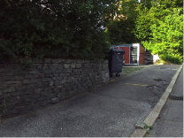
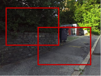
w/o crop	random crop	R2 crop

Figure 2: Comparisons among different crop augmentations. As for R² crop, we utilize different colors to indicate that we adopt randomly selected size of crop patches.

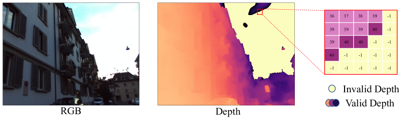
Figure 3: Illustration of invalid depth GT pixels in the dataset. These pixels appear not only in the sky areas but also in close positions where the sensor cannot provide reliable GT value. We highlight a training sample for a clear Introduction of our valid mask in gradloss in Fig. 4.

3.2 R² Crop

Data augmentation is crucial to training models with better performance. Typically, the sequence of data augmentation for monocular depth estimation includes random rotation, random flip, random crop, and random color enhancement [21]. We propose the more effective crop strategy R² crop, in which we randomly select the size of crop patches and the cropped locations. We highlight the discrepancy with other commonly used crop methods in Fig. 2. It increases the diversity of the scenes and effectively avoids overfitting the training set.

3.3 Multiple Loss Training

Previous depth estimation methods [20, 5, 24, 25] only adopt the silog loss to train the neural network:

$$\mathcal{L}_{silog}=\alpha\sqrt{\frac{1}{N}\sum\limits_{i}^{N}e_{i}^{2}-\frac{\lambda}{N^{2}}(\sum\limits_{i}^{N}e_{i})^{2}},$$ (7)

where $e_{i}=\log\hat{d}_{i}-\log d_{i}$ with the ground truth depth $d_{i}$ and predicted depth $\hat{d}_{i}$. $N$ denotes the number of pixels having valid ground truth values. Since we discover that the lightweight model supervised by this simple single loss lacks representation capability and is easily stuck in local optimal, we adopt diverse loss terms to provide various targets for sufficient model training.

Motivated by [34], we first propose a gradience loss $\mathcal{L}_{grad}$ formulated as:

$$\mathcal{L}_{grad}=\frac{1}{N}\sum_{i}\left(M_{x_{i}}\times\left\|\nabla_{x}\hat{d}_{i}-\nabla_{x}d_{i}\right\|_{1}+M_{y_{i}}\times\left\|\nabla_{y}\hat{d}_{i}-\nabla_{y}d_{i}\right\|_{1}\right),$$ (8)

where $\nabla$ is the gradience calculation operation. Since the gradience loss is calculated in a dislocation subtraction manner and there are tremendous invalid depth GT in the dataset as shown in Fig. 3, as presented in Fig. 4, simply applying gradience calculation will blemish the information of invalid pixels and introduce outlier values when calculating the loss term. Hence, it is necessary to carefully design a strategy to calculate masks $M$ to filter these invalid pixels in $\mathcal{L}_{grad}$. To solve this issue, we first replace the invalid value with NaN and then calculate the GT for gradience loss. Thanks to the numeral property of NaN and Inf, invalid information can be reserved. Consequently, we can filter the NaN and Inf when calculating the gradience loss.

Moreover, we also adopt the virtual norm loss $\mathcal{L}_{vnl}$ [43], and robust loss $\mathcal{L}_{robust}$ [4]. We formulate them as follows:

$$\mathcal{L}_{vnl}=\frac{1}{N}\sum\limits_{i}^{N}\left\|\hat{n}_{i}-n_{i}\right\|_{1},$$ (9)

where $n$ is the virtual norm. We refer more details in the original paper [43]. Unlike the original implementation, we sample points from reconstructed point clouds and adopt constraints on predictions to filter invalid samples instead of ground truth. It helps the model convergence at the beginning of training.

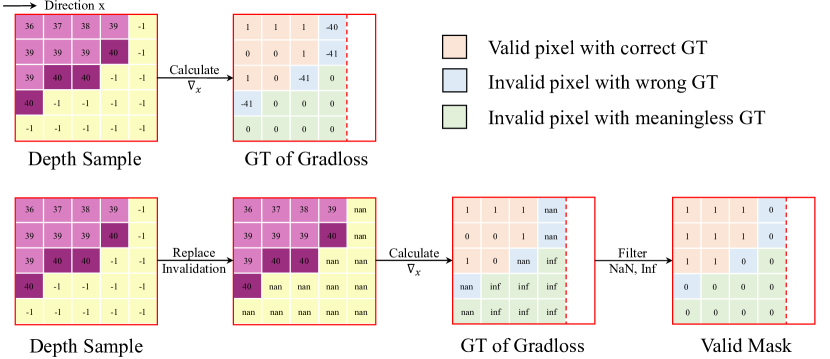
Figure 4: Illustration of valid mask calculation for gradience loss (x direction). First line: vanilla calculation of gradience loss. Second line: we propose to first replace invalid value with NaN and compute reasonable valid mask for gradience loss.

$$\mathcal{L}_{robust}=\frac{1}{N}\sum\limits_{i}^{N}\frac{|\alpha-2|}{\alpha}\left(\left(\frac{(e_{i}/c)^{2}}{|\alpha-2|}\right)^{\alpha/2}-1\right),$$ (10)

where $e_{i}=\hat{d}_{i}-d_{i}$. We experimentally set $\alpha=1$ and $c=2$. In fact, the loss reduces to a simple $L_{2}$ loss, but which is proven to be more effective compared with the proposed adaptive version in our task. More experiments can be conducted to decide a better choice for $\alpha$ and $c$.

Finally, we adopt a combination of these loss terms to train our network. The total depth loss is

$$\mathcal{L}_{depth}=w_{1}\mathcal{L}_{silog}+w_{2}\mathcal{L}_{grad}+w_{3}\mathcal{L}_{vnl}+w_{4}\mathcal{L}_{robust}.$$ (11)

We set $w_{1}=1$, $w_{2}=0.25$, $w_{3}=2.5$, and $w_{4}=0.6$ based on tremendous experiments. Then, we apply a dynamic re-weight strategy in which the loss weights $w$ are set as model parameters and are automatically fine-tuned during the training stage. Experimental results indicate that this strategy can achieve similar results as tuning the weights by hand.

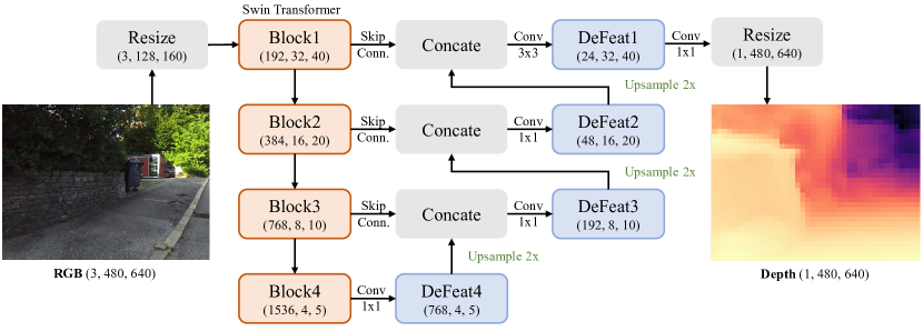
Figure 5: Illustration of the teacher network.

3.4 Structure-Aware Distillation

We apply the structure-aware distillation strategy [27, 38] to further boost model performance. For the teacher model, we choose Swin Transformer [28] as the encoder and adopt a similar lightweight decoder to recover featrue resolution and predict depth maps. We present the network architecture in Fig. 5. The teacher model is trained via the supervision of $\mathcal{L}_{depth}$ and is then fixed when distilling the student model. During the distillation, multi-level distlling losses are adopted to provide supervisons on immediate features as shown in Fig. 6. The distillation loss is formulated as

$$\mathcal{L}_{distill}=\sum\limits_{l}^{L}\left(\frac{1}{H\times W}\sum\limits_{i}^{H}\sum\limits_{j}^{W}\left\|a_{ij}^{s}-a_{ij}^{t}\right\|_{1}\right),$$ (12)

where $a$ is the affinity map calculated via inner-product of $L_{2}$ normalized features. We refer to [27, 38] for more details. $s$ and $t$ indicate the features are from the student and teacher model, respectively. We choose three level ($L=3$) features for distll, which are DeFeat2, DeFeat3, and DeFeat4 in Fig. 1.

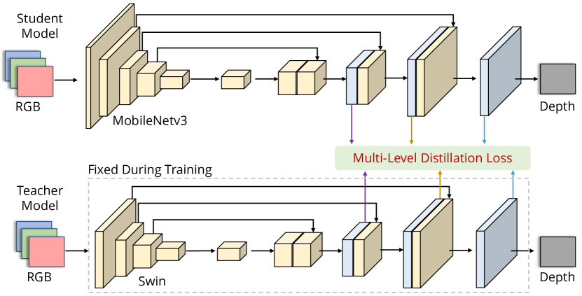
Figure 6: Illustration of our multi-scale distillation strategy.

Consequently, the student model is trained via the total loss $\mathcal{L}$:

$$\mathcal{L}=\mathcal{L}_{depth}+w_{d}\mathcal{L}_{distill},$$ (13)

where $w_{d}=10$ in our experiments. Notably, unlike previous work [27, 38], we adopt a two-stage training paradigm. During the first stage, the student model is only trained via $\mathcal{L}_{depth}$. In the second stage, we adopt the teacher model and utilize the total loss $\mathcal{L}$ to further boost the performance of the student model.

4 Experiments

In this section, we introduce our experiments to evaluate the effectiveness of our solution. We first elaborate the dataset and define the evaluation metrics. Then the detailed implementation and ablation studies are presented. We also report the inference time on target devices (i.e., Raspberry Pi 4) to show that our method can not only produce reasonable depth estimation but also achieve real-time inference on resource-constrained hardware.

4.1 Setup

4.1.1 Dataset

We utilize the dataset provided by MAI&AIM2022 challenge to conduct experiments, which contains 7385 pairs of RGB and grayscale depth images. The pixel values of depth maps are in uint16 format ranging from 0 to 40000, which represent depth values from 0 to 40 meters. We use 6869 pairs for training and the rest 516 pairs as the local validation set.

4.1.2 Evaluation Metrics

In MAI&AIM2022 challenge [18], two metrics are considered for each submission solution: 1) The quality of the depth estimation. It is measured by the invariant standard root mean squared error (si-RMSE). 2) The runtime of the model on the target platform (i.e., Raspberry Pi 4). The scoring formulation is provided below:

$$\text{Score}(\text{si-RMSE},\text{runtime})=\frac{2^{-20}\cdot\text{si-RMSE}}{C\cdot\text{runtime}},$$ (14)

where $C=0.01$ on the online validation benchmark.

4.2 Implementation Details

We implement the proposed model via the monocular depth estimation toolbox [21], which is based on the open-source machine learning library Pytorch. The model is converted to TFLite [26] after training. We use Adam optimizer with betas = (0.9, 0.999) and eps=1e-3. A poly schedule is adopted where the base learning rate is 4e^-3 and the power is 0.9. The total number of epochs is 600 with batch size = 32 on two RTX3090 GPUs, which takes around 4 hours to train a model. The encoder of our network is pretrained on ImageNet, and the decoder part is trained from scratch.

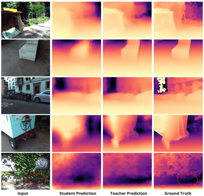
Figure 7: The visualization results of our proposed methods. One can observe that there is noise in ground truth labels which we highlight with a red circle.

4.3 Quantitative Results

As shown in Tab. 1, our proposed method achieves a score of 232.04 on the challenge test set and ranks second place. Our solution achieves 0.311 si-RMSE with 37$ms$ on the Raspberry Pi 4. Notably, our runtime is lower than the other methods and the performance is comparable.

4.4 Qualitative Results

We visualize the prediction results of our proposed methods as shown in Fig. 7, which demonstrates that our methods can achieve reasonable depth estimation results. However, the predicted depth maps are very rough around the edges due to the excessive down-sampling.

4.5 Inference Time

In this section, we verify that our method can achieve high-throughput monocular depth estimation on mobile devices. We convert our model to TensorFlow-Lite and test the inference time on various mobile devices, including smartphones with Kirin 980 and Snapdragon 7 Gen 1. We test the model using AI Benchmark [16, 17]. Following the challenge requirements, the resolution of input and output images is 640$\times$480. The data type is set to float (32 bit). As presented in Tab 2, our network can obtain extremely high-throughput inference. It achieve 162FPS on smart phones with Snapdragon 7 Gen 1 processor. Interestingly, we can observe that the model is CPU-friendly, with an even faster inference on CPU than GPU on mobile devices.

Table 2: Inference time of our network (AI Benchmark).

SoC Device Average/ms   STD/ms Kirin 980 CPU 6.85 0.77 Kirin 980 GPU Delegate 9.84 0.66 Snapdragon 7 Gen 1 CPU 6.16 1.71 Snapdragon 7 Gen 1 GPU Delegate 7.17 1.00

4.6 Ablation Studies

4.6.1 Effectiveness of Network Design

Encoder selection is crucial to the trade-off between fidelity and runtime. We recommend refering [15, 38] for more comparisons among various encoders. Following these works, we choose the MobileNet-v3 as the default encoder. We then present comparisons among different decoder designs as shown in Tab. 3. Typically, previous methods [15, 38, 20, 5, 24] utilize the 3$\times$3 convolution to fuse features. While the quantitative results are good, the runtime can be longer. However, when we replace all the 3$\times$3 convolution with 1$\times$1 convolution, the model performance drops drastically while the runtime gets short. Hence, we adopt a mix version as presented in our Sec. 3.1 and Fig. 1. We utilize a 3$\times$3 convolution at the highest resolution and adopt 1$\times$1 convolutions at other places, which makes the best trade-off between fidelity and runtime, getting the highest score on the benchmark. We then present the importance of the merging image normalization. It significantly reduces the runtime without any performance drop.

Table 3: Ablation study about the network architecture design. Dec and MIN are the short for decoder and merge image normalization, respectively.

Architecture    MIN   si-RMSE Runtime/ms    Score Full 3$\times$3 @ Dec. 0.295 62 27.01 Full 1$\times$1 @ Dec. 0.308 53 26.38 Mix Convs @ Dec. 0.301 56 27.51 Mix Convs @ Dec. ✓ 0.301 37 41.64

4.6.2 Effectiveness of R² Crop

We present the ablation study of various crop strategies. In these experiments, we only adopt the single sigloss (Eq. 7) for simplicity. As shown in Tab. 4, our proposed R² crop indicates an engaging improvement on performance compared with the baseline methods. When we adopt the vanilla random crop, the model cannot learn the knowledge of full-area images. However, the model infers on full-area images during the validation stage. This discrepancy leads to significant performance degradation. If we do not apply any crop strategy, the diversity of training samples is limited, also leading to a performance limitation. When we adopt our proposed R² crop, during the training stage, the model can not only learn the knowledge of full-area images but also ensure the diversity of training samples. When increasing the variety of crop sizes, the model performance can be improved simultaneously. However, too small patches cannot bring performance gains but lead to a slight degradation (e.g., (144, 256) patches in our ablation study). We infer that the small patches do not contain sufficient structure information for facilitating the model training. As a result, we adopt patches with a size of [(240, 384), (384, 512), (480, 640)] in our solution.

Table 4: Ablation study of crop strategies. (h, w) represents the size of crop patches.

Method   si-RMSE RMSE w/o crop 0.335 4.25 random crop with (384, 512) 0.377 4.62 R² crop with [(384, 512), (480, 640)] 0.327 4.15 R² crop with [(240, 384), (384, 512), (480, 640)] 0.323 4.11 R² crop with [(144, 256), (240, 384), (384, 512), (480, 640)] 0.325 4.13

4.6.3 Effectiveness of Multiple-Loss Training

This section evaluates the effectiveness of each loss term used in our solution. The results are presented in Tab. 5. Each loss term can bring performance gains for the model. We also highlight that if we do not apply the invalid mask in gradience loss, the model convergence will be hurt as described in Sec. 3.3. Moreover, our dynamic weight strategy can also achieve satisfactory results without fine-tuning loss weights by hand. We utilize the handcrafted weights as a default setting to achieve a better score in the challenge.

Table 5: Ablation study of the multiple loss strategy.

Sig Loss (Eq. 7) Grad Loss (Eq. 8) VNL Loss (Eq. 9) Robust Loss (Eq. 10) Dynamic Weight   si-RMSE ✓ 0.323 ✓ ✓ 0.316 ✓ ✓ ✓ 0.309 ✓ ✓ ✓ ✓ 0.303 ✓ ✓ ✓ ✓ ✓ 0.306

4.6.4 Effectiveness of Distillation

We first present the results of the teacher model. As shown in Tab. 6, the teacher model achieves much better fidelity compared to the student model. It indicates that there is improvement room for the student model to learn from the teacher model via the distillation. We also present qualitative results in Fig. 7 for intuitive comparisons. As we can observe from the predicted depth maps, the teacher model provides more reasonable and sharper depth estimation results.

We then evaluate different distillation strategies in this section. Motivated by previous work, we try to apply L2 distillation [15], structure-aware distillation [27, 38], and channel-wise distillation [33]. Interestingly, all strategies cannot directly work well for our lightweight student model as presented in Tab. 6. One possible reason is that we adopt multiple loss terms, leading to difficulty in balancing the loss weights. However, we also conduct experiments in which we only adopt the single sigloss and apply the distillation strategies. The results are similar without improvement in model performance. Moreover, some distillation strategies conflict with the two-stage fine-tuning, leading to a convergence issue. These experimental results indicate that more effective distillation strategies should be designed for monocular depth estimation. In this solution, we propose to adopt structure-aware distillation. It brings a slight improvement to the si-RMSE of our lightweight student model but a degradation on RMSE, indicating there is still huge room to improve the distillation strategy.

Table 6: Ablation study of distillation strategies. Two-Stage indicates applying the distillation in a fine-tuning manner. $\varnothing$ denotes that the fine-tuning process does not converge.

Method   Two-Stage   si-RMSE RMSE Teacher Model 0.228 3.025 Baseline Student Model 0.303 3.785 L2 Distillation 0.307 3.978 L2 Distillation ✓     $\varnothing$ Channel-Wise Distillation 0.311 4.045 Channel-Wise Distillation ✓     $\varnothing$ Structure-Aware Distillation 0.306 3.994 Structure-Aware Distillation ✓ 0.301 3.839

5 Conclusion

We have introduced our solution for fast and accurate depth estimation on mobile devices. Specifically, we design an extremely lightweight model for depth estimation. Then, we propose R² crop to enrich the diversity of training samples. To facilitate the model training, we design a gradience loss and adopt multiple-loss items. We also investigate various distillation strategies. Extensive experiments indicate the effectiveness of our proposed solution.

6 Acknowledgments

The research was supported by the National Natural Science Foundation of China (61971165, 61922027), and also is supported by the Fundamental Research Funds for the Central Universities.

References

- [1] Huawei hiai engine introduction. https://developer.huawei.com/consumer/en/doc/2020315 (2018)
- [2] Snapdragon neural processing engine sdk. https://developer.qualcomm.com/docs/snpe/overview.html (2018)
- [3] Armbrüster, C., Wolter, M., Kuhlen, T., Spijkers, W., Fimm, B.: Depth perception in virtual reality: distance estimations in peri-and extrapersonal space. Cyberpsychology & Behavior 11(1), 9–15 (2008)
- [4] Barron, J.T.: A general and adaptive robust loss function. In: CVPR. pp. 4331–4339 (2019)
- [5] Bhat, S.F., Alhashim, I., Wonka, P.: Adabins: Depth estimation using adaptive bins. In: CVPR. pp. 4009–4018 (2021)
- [6] Chen, Z., Li, Z., Zhang, S., Fang, L., Jiang, Q., Zhao, F., Zhou, B., Zhao, H.: Autoalign: Pixel-instance feature aggregation for multi-modal 3d object detection. arXiv preprint arXiv:2201.06493 (2022)
- [7] Chen, Z., Li, Z., Zhang, S., Fang, L., Jiang, Q., Zhao, F.: Autoalignv2: Deformable feature aggregation for dynamic multi-modal 3d object detection. arXiv preprint arXiv:2207.10316 (2022)
- [8] Chen, Z., Li, Z., Zhang, S., Fang, L., Jiang, Q., Zhao, F.: Graph-detr3d: Rethinking overlapping regions for multi-view 3d object detection. arXiv preprint arXiv:2204.11582 (2022)
- [9] Eigen, D., Puhrsch, C., Fergus, R.: Depth map prediction from a single image using a multi-scale deep network. NeurIPS (2014)
- [10] Fu, H., Gong, M., Wang, C., Batmanghelich, K., Tao, D.: Deep ordinal regression network for monocular depth estimation. In: CVPR. pp. 2002–2011 (2018)
- [11] Gerig, N., Mayo, J., Baur, K., Wittmann, F., Riener, R., Wolf, P.: Missing depth cues in virtual reality limit performance and quality of three dimensional reaching movements. PLoS one 13(1), e0189275 (2018)
- [12] Godard, C., Mac Aodha, O., Firman, M., Brostow, G.J.: Digging into self-supervised monocular depth estimation. In: ICCV. pp. 3828–3838 (2019)
- [13] Hazirbas, C., Ma, L., Domokos, C., Cremers, D.: Fusenet: Incorporating depth into semantic segmentation via fusion-based cnn architecture. In: ACCV. pp. 213–228. Springer (2016)
- [14] Howard, A.G., Zhu, M., Chen, B., Kalenichenko, D., Wang, W., Weyand, T., Andreetto, M., Adam, H.: Mobilenets: Efficient convolutional neural networks for mobile vision applications. arXiv preprint arXiv:1704.04861 (2017)
- [15] Ignatov, A., Malivenko, G., Plowman, D., Shukla, S., Timofte, R.: Fast and accurate single-image depth estimation on mobile devices, mobile ai 2021 challenge: Report. In: CVPR. pp. 2545–2557 (2021)
- [16] Ignatov, A., Timofte, R., Chou, W., Wang, K., Wu, M., Hartley, T., Van Gool, L.: Ai benchmark: Running deep neural networks on android smartphones. In: Proceedings of the European Conference on Computer Vision (ECCV) Workshops. pp. 0–0 (2018)
- [17] Ignatov, A., Timofte, R., Kulik, A., Yang, S., Wang, K., Baum, F., Wu, M., Xu, L., Van Gool, L.: Ai benchmark: All about deep learning on smartphones in 2019. In: ICCVW. pp. 3617–3635. IEEE (2019)
- [18] Ignatov, A., Timofte, R., et al.: Efficient single-image depth estimation on mobile devices, mobile ai & aim 2022 challenge: Report. In: ECCV (2022)
- [19] Kim, D., Ga, W., Ahn, P., Joo, D., Chun, S., Kim, J.: Global-local path networks for monocular depth estimation with vertical cutdepth. arXiv preprint arXiv:2201.07436 (2022)
- [20] Lee, J.H., Han, M.K., Ko, D.W., Suh, I.H.: From big to small: Multi-scale local planar guidance for monocular depth estimation. arXiv preprint arXiv:1907.10326 (2019)
- [21] Li, Z.: Monocular depth estimation toolbox. https://github.com/zhyever/Monocular-Depth-Estimation-Toolbox (2022)
- [22] Li, Z., Chen, Z., Li, A., Fang, L., Jiang, Q., Liu, X., Jiang, J.: Unsupervised domain adaptation for monocular 3d object detection via self-training. arXiv preprint arXiv:2204.11590 (2022)
- [23] Li, Z., Chen, Z., Li, A., Fang, L., Jiang, Q., Liu, X., Jiang, J., Zhou, B., Zhao, H.: Simipu: Simple 2d image and 3d point cloud unsupervised pre-training for spatial-aware visual representations. arXiv preprint arXiv:2112.04680 (2021)
- [24] Li, Z., Chen, Z., Liu, X., Jiang, J.: Depthformer: Exploiting long-range correlation and local information for accurate monocular depth estimation. arXiv preprint arXiv:2203.14211 (2022)
- [25] Li, Z., Wang, X., Liu, X., Jiang, J.: Binsformer: Revisiting adaptive bins for monocular depth estimation. arXiv preprint arXiv:2204.00987 (2022)
- [26] Lite, T.: Deploy machine learning models on mobile and iot devices (2019)
- [27] Liu, Y., Shu, C., Wang, J., Shen, C.: Structured knowledge distillation for dense prediction. IEEE TPAMI (2020)
- [28] Liu, Z., Lin, Y., Cao, Y., Hu, H., Wei, Y., Zhang, Z., Lin, S., Guo, B.: Swin transformer: Hierarchical vision transformer using shifted windows. ICCV (2021)
- [29] Park, D., Ambrus, R., Guizilini, V., Li, J., Gaidon, A.: Is pseudo-lidar needed for monocular 3d object detection? In: ICCV. pp. 3142–3152 (2021)
- [30] Patil, V., Sakaridis, C., Liniger, A., Van Gool, L.: P3depth: Monocular depth estimation with a piecewise planarity prior. In: CVPR. pp. 1610–1621 (2022)
- [31] Reading, C., Harakeh, A., Chae, J., Waslander, S.L.: Categorical depth distribution network for monocular 3d object detection. In: Proceedings of the IEEE/CVF Conference on Computer Vision and Pattern Recognition. pp. 8555–8564 (2021)
- [32] Ronneberger, O., Fischer, P., Brox, T.: U-net: Convolutional networks for biomedical image segmentation. In: MICCAI. pp. 234–241. Springer (2015)
- [33] Shu, C., Liu, Y., Gao, J., Yan, Z., Shen, C.: Channel-wise knowledge distillation for dense prediction. In: ICCV. pp. 5311–5320 (2021)
- [34] Sitzmann, V., Martel, J., Bergman, A., Lindell, D., Wetzstein, G.: Implicit neural representations with periodic activation functions. NeurIPS 33, 7462–7473 (2020)
- [35] Vu, T.H., Jain, H., Bucher, M., Cord, M., Pérez, P.: Dada: Depth-aware domain adaptation in semantic segmentation. In: ICCV. pp. 7364–7373 (2019)
- [36] Wang, T., Pang, J., Lin, D.: Monocular 3d object detection with depth from motion. arXiv preprint arXiv:2207.12988 (2022)
- [37] Wang, W., Neumann, U.: Depth-aware cnn for rgb-d segmentation. In: ECCV. pp. 135–150 (2018)
- [38] Wang, Y., Li, X., Shi, M., Xian, K., Cao, Z.: Knowledge distillation for fast and accurate monocular depth estimation on mobile devices. In: CVPR. pp. 2457–2465 (2021)
- [39] Wang, Y., Guizilini, V.C., Zhang, T., Wang, Y., Zhao, H., Solomon, J.: Detr3d: 3d object detection from multi-view images via 3d-to-2d queries. In: Conference on Robot Learning. pp. 180–191. PMLR (2022)
- [40] Weng, X., Kitani, K.: Monocular 3d object detection with pseudo-lidar point cloud. In: Proceedings of the IEEE/CVF International Conference on Computer Vision Workshops. pp. 0–0 (2019)
- [41] Wofk, D., Ma, F., Yang, T.J., Karaman, S., Sze, V.: Fastdepth: Fast monocular depth estimation on embedded systems. In: ICRA. pp. 6101–6108. IEEE (2019)
- [42] Yang, G., Tang, H., Ding, M., Sebe, N., Ricci, E.: Transformers solve the limited receptive field for monocular depth prediction. In: ICCV (2021)
- [43] Yin, W., Liu, Y., Shen, C., Yan, Y.: Enforcing geometric constraints of virtual normal for depth prediction. In: ICCV. pp. 5684–5693 (2019)
- [44] You, Z., Tsai, Y.H., Chiu, W.C., Li, G.: Towards interpretable deep networks for monocular depth estimation. In: ICCV. pp. 12879–12888 (2021)
- [45] Zhou, T., Brown, M., Snavely, N., Lowe, D.G.: Unsupervised learning of depth and ego-motion from video. In: CVPR. pp. 1851–1858 (2017)
- [46] Zhu, S., Brazil, G., Liu, X.: The edge of depth: Explicit constraints between segmentation and depth. In: CVPR. pp. 13116–13125 (2020)