TOSE: A Fast Capacity Estimation Algorithm Based on Spike Approximations

Abstract

Capacity is one of the most important performance metrics for wireless communication networks. It describes the maximum rate at which the information can be transmitted of a wireless communication system. To support the growing demand for wireless traffic, wireless networks are becoming more dense and complicated, leading to a higher difficulty to derive the capacity. Unfortunately, most existing methods for the capacity calculation take a polynomial time complexity. This will become unaffordable for future ultra-dense networks, where both the number of base stations (BSs) and the number of users are extremely large. In this paper, we propose a fast algorithm TOSE to estimate the capacity for ultra-dense wireless networks. Based on the spiked model of random matrix theory (RMT), our algorithm can avoid the exact eigenvalue derivations of large dimensional matrices, which are complicated and inevitable in conventional capacity calculation methods. Instead, fast eigenvalue estimations can be realized based on the spike approximations in our TOSE algorithm. Our simulation results show that TOSE is an accurate and fast capacity approximation algorithm. Its estimation error is below 5%, and it runs in linear time, which is much lower than the polynomial time complexity of existing methods. In addition, TOSE has superior generality, since it is independent of the distributions of BSs and users, and the shape of network areas.

I Introduction

Capacity can be regarded as one of the most important performance metrics of wireless communication networks. Capacity determination for future wireless networks is also listed as one of the ten most challenging information and communication technology (ICT) problems in the post-Shannon era [1]. With the rapid development of mobile communication technology, wireless systems become more and more complicated, leading to a higher complexity in determining the capacity. In 1948, Dr. Claude E. Shannon defined the notion of channel capacity and provided a mathematical model to compute the capacity [2]. According to the Shannon-Hartley theorem, the capacity of an additive white Gaussian noise (AWGN) channel can be determined according to $C=W\log(1+\frac{P}{N_{0}W})$ [3], where $W$ is the channel bandwidth, $P$ is the signal power and $N_{0}$ is the power of AWGN. Then, the technique of multiple-input and multiple-output (MIMO) was proposed for multiplying the capacity of a wireless channel. For a multi-user (MU)-MIMO channel with $t$ transmission antennas and $r$ receiving antennas, its uplink channel capacity can be determined according to [4], as:

$$C=\mathbb{E}\{\log\det(\mathbf{I}+\frac{P}{t}\mathbf{H}\mathbf{H}^{*})\},\vspace{-0.2em}$$ (1)

where $\mathbf{H}$ denotes the channel gain matrix, and $\mathbf{H}^{*}$ is the Hermitian transpose of $\mathbf{H}$. The notation $\mathbb{E}$ represents the expectation. Note that (1) is the capacity for a single MU-MIMO channel. Then what is the capacity for a wireless system with multiple MU-MIMO channels?

For a huge and ultra-dense wireless network, if all the base stations (BSs) are fully cooperated to serve all the users, the signaling overhead will be extremely large and the whole network will become unscalable [5, 6]. To avoid these problems, the whole network can be divided into multiple clusters [7, 8, 9, 10]. Each cluster contains multiple closely-located BSs serving nearby users cooperatively. Then the wireless channel of each cluster can thus be modeled as a MU-MIMO channel. The whole network with multiple non-overlapping clusters can be regarded as a system with multiple MU-MIMO channels, with interference exiting among different channels. According to [8], the average capacity of the $m$-th cluster per BS can be calculated according to

$$C_{m}\!=\!\mathbb{E}\!\left\{\!\frac{1}{J_{m}}\!\log\det\left[\mathbf{I}\!+\!P(N_{0}\mathbf{I}\!+\!P\mathbf{\Pi}_{m}\mathbf{\Pi}_{m}^{*})^{-1}\mathbf{H}_{m}\mathbf{H}_{m}^{*}\right]\!\right\}\!,$$ (2)

where $J_{m}$ denotes the number of BSs of cluster $m$. $\mathbf{H}_{m}$ is the channel gain matrix of cluster $m$, and $\mathbf{\Pi}_{m}$ is the interference matrix of cluster $m$, which will be specified later in Section II. Note that (2) is more general than (1), and thus we will focus on (2) in the following parts.

There exist many different methods to calculate the capacity based on (2). The most direct way is to calculate the matrix determinant, through conventional schemes, such as singular value decomposition (SVD) and Cholesky decomposition, etc. It should be noticed that such conventional determinant-calculation-based methods take a polynomial time to derive the capacity. Such a time complexity is obviously unacceptable for future ultra-dense networks. Another method, which is applicable for ultra-dense networks, was developed by Tulino and Verdu [11]. They made use of the random matrix theory (RMT) to estimate the wireless channel capacity. However, they mainly focused on the point-to-point channels with the code-division multiple access (CDMA) scheme, and their derived capacity expressions are still implicit and complex. An efficient and general method to derive the capacity for ultra-dense networks is still missing.

In this paper, we propose a Top-N-Simulated-Estimations (TOSE) algorithm to estimate $C_{m}$, which is fast, accurate, and general. Specifically, we realize the eigenvalue estimation of a large channel gain matrix based on the spiked model in RMT, and then the matrix determinant in (2) can be derived with a low complexity. As such, the complicated eigenvalue derivation steps (e.g., SVD or Cholesky decomposition) in conventional determinant-calculation-based methods can be totally avoided. It should be noticed that our TOSE algorithm is designed based on the spike approximations in RMT, which is not utilized in the conventional RMT-based methods [11]. Besides of the low complexity, our algorithm has a high accuracy on capacity estimation, with the estimation error below 5%. Thus, for the ultra-dense wireless networks, where the number of network nodes (e.g., BSs and users) are large, TOSE has a huge efficiency advantage. Third, our TOSE algorithm has superior generality, since it is independent of the distribution of network nodes, and the shape of the network area.

II System model and Baseline Algorithm

II-A System Model and Capacity Formula

Consider a wireless network with $J$ single-antenna BSs and $K$ single-antenna users. The set of BSs is denoted as $\mathcal{S}=\{s_{1},s_{2},\dots s_{J}\}$, and the set of users is denoted as $\mathcal{U}=\{u_{1},u_{2},\dots,u_{K}\}$. The network is organized into $M$ non-overlapping clusters, and we use $\mathcal{C}_{m}$ to denote the $m$-th cluster. Then we have $\mathcal{S}\bigcup\mathcal{U}=\bigcup_{m=1}^{M}\mathcal{C}_{m}$ [8]. The sets of the BSs and the users in $\mathcal{C}_{m}$ are denoted by $\mathcal{S}_{m}=\mathcal{S}\bigcap\mathcal{C}_{m}$ and $\mathcal{U}_{m}=\mathcal{U}\bigcap\mathcal{C}_{m}$, respectively. Moreover, we use $J_{m}=|\mathcal{S}_{m}|$ and $K_{m}=|\mathcal{U}_{m}|$ to denote the number of BSs and users in $\mathcal{C}_{m}$. In this work, we focus on the ultra-dense scenario, and thus assume $J_{m},\;K_{m}\to\infty\;(m=1,2,\cdots,M)$ [8].

Define the channel gain between the BS $s_{j}\in\mathcal{S}_{m}$ and the user $u_{k}\in\mathcal{U}$ as

$$\vspace{-0.2em}h_{mjk}=l_{mjk}g_{mjk},\vspace{-0.2em}$$

where $g_{mjk}\sim\mathcal{CN}(0,1)$ is the small-scale fading and

$$l_{mjk}=\left\{\begin{array}[]{ll}d_{mjk}^{-1.75},&d_{mjk}>d_{1},\\ d_{1}^{-0.75}d_{mjk}^{-1},&d_{0}<d_{mjk}\leq d_{1},\\ d_{1}^{-0.75}d_{0}^{-1},&d_{mjk}\leq d_{0}\end{array}\right.\vspace{-0.2em}$$ (3)

is the large-scale fading [9]. Here, $d_{mjk}$ represents the Euclidean distance between the BS $s_{j}\in\mathcal{S}_{m}$ and the user $u_{k}\in\mathcal{U}$. The parameters $d_{0}$ and $d_{1}$ are the near field threshold and far field threshold, respectively.

Thus, we can define the large-scale fading matrix $\mathbf{L}_{m}\in\mathbb{R}^{J_{m}\times K_{m}}$ and the small-scaling fading matrix $\mathbf{G}_{m}\in\\ \mathbb{C}^{J_{m}\times K_{m}}$, with their $(j,k)$-th entry given by

$$[\mathbf{L}_{m}]_{jk}=l_{mjk},\quad[\mathbf{G}_{m}]_{jk}=g_{mjk},\vspace{-0.2em}$$

where the BS $s_{j}\in\mathcal{S}_{m}$ and the user $u_{k}\in\mathcal{U}_{m}$. The channel gain matrix $\mathbf{H}_{m}$ in (2) can thus be defined as

$$\mathbf{H}_{m}=\mathbf{L}_{m}\circ\mathbf{G}_{m},\vspace{-0.2em}$$ (4)

where $\circ$ denotes the Hadamard product. The interference matrix $\mathbf{\Pi}_{m}$ in (2) can be similarly defined as a Hadamard product of a large-scale fading matrix and a small-scale fading matrix, but these two fading matrices contain the users outside of $\mathcal{C}_{m}$ and the BSs inside $\mathcal{C}_{m}$, namely, $u_{k}\in\mathcal{U}\setminus\mathcal{U}_{m}$, and $s_{j}\in\mathcal{S}_{m}$. Details of deriving $\mathbf{\Pi}_{m}$ can be found in [10], and we omit its elaboration here due to space limitation. To further analyze (2), we define

$$\mathbf{\Xi}_{m}=N_{0}\mathbf{I}+P\mathbf{\Pi}_{m}\mathbf{\Pi}_{m}^{*}\vspace{-0.2em}$$ (5)

as the noise-plus-interference matrix, with $\mathbf{\Xi}_{m}\in\mathbb{C}^{J_{m}\times J_{m}}$. Based on Lemma 1 in [10], we know that $\mathbf{\Xi}_{m}$ converges to a positive definite diagonal matrix as $J_{m}$ and $K-K_{m}$ approach infinity, namely,

$$\mathbf{\Xi}_{m}=\textrm{diag}((N_{0}+P\xi_{11}^{m}),\dots,(N_{0}+P\xi_{J_{m}J_{m}}^{m})),$$ (6)

where $\xi_{jj}^{m}=\sum_{u_{k}\in\mathcal{U}\setminus\mathcal{U}_{m}}l_{mjk}^{2}$. Thus, (2) can be transformed into

$$C_{m} =\mathbb{E}\left\{\frac{1}{J_{m}}\log\det\left(\mathbf{I}+P\mathbf{\Xi}_{m}^{-1/2}\mathbf{H}_{m}\mathbf{H}_{m}^{*}\mathbf{\Xi}_{m}^{-1/2}\right)\right\}$$

$$=\mathbb{E}\left\{\frac{1}{J_{m}}\log\det[\mathbf{I}+\left(\mathbf{Q}_{m}\circ\mathbf{G}_{m}\right)\left(\mathbf{Q}_{m}\circ\mathbf{G}_{m}\right)^{*}]\right\},\vspace{-0.2em}$$ (7)

where $\mathbf{Q}_{m}=P^{1/2}\mathbf{\Xi}_{m}^{-1/2}\mathbf{L}_{m}$. In the following, we will focus on the computation of $C_{m}$ based on (7).

II-B Baseline Algorithm Based on Cholesky Decomposition

It can be observed from (7) that, the most direct way to calculate $C_{m}$ is to compute the logarithm of the determinant of the following matrix

$$\mathbf{I}+(\mathbf{Q}_{m}\circ\mathbf{G}_{m})(\mathbf{Q}_{m}\circ\mathbf{G}_{m})^{*},$$

and then to obtain its average value. Since the above matrix is Hermitian positive-definite, a classical approach to derive its determinant is to use the Cholesky decomposition, namely,

$$\mathbf{I}+(\mathbf{Q}_{m}\circ\mathbf{G}_{m})(\mathbf{Q}_{m}\circ\mathbf{G}_{m})^{*}=\mathbf{R}_{m}\mathbf{R}_{m}^{*},$$ (8)

where $\mathbf{R}_{m}$ is a lower triangular matrix with real and positive diagonal entries $r_{11}^{m},\;r_{22}^{m},\cdots,r_{J_{m}J_{m}}^{m}$ [12]. As such, (7) becomes

$$C_{m}\!=\!2\mathbb{E}\left\{\frac{1}{J_{m}}\log\det\left(\mathbf{R}_{m}\right)\right\}=\!2\mathbb{E}\left\{\frac{1}{J_{m}}\sum_{j=1}^{J_{m}}\log r^{m}_{jj}\right\}.\vspace{-0.2em}$$ (9)

It is well known that the flops of the Cholesky decomposition are $J_{m}^{3}/3$ [14]. This is obviously an unaffordable time complexity for ultra-dense networks, where $J_{m}$ is extremely large. However, such a time complexity is difficult to improve further if we still choose such a direct method, by calculating the logarithm of the determinant of a large random matrix, to derive the capacity. Thus, there is a strong motivation to develop a new method for fast capacity estimation.

III TOSE Algorithm Design

In this section, we will elaborate our TOSE algorithm for fast capacity estimation. We first propose an approximation of $C_{m}$, denoted by $\widehat{C}_{m}$, by replacing the Hadamard product in (7) with the matrix product. Second, we obtain an estimation of $\widehat{C}_{m}$ through fast eigenvalue approximations based on the spiked model in RMT, with which the complicated steps to calculate the exact eigenvalues can be avoided. Since the top $N$ spiked eigenvalues can be estimated, we name our algorithm Top-N-Simulated-Estimations (TOSE).

III-A Transformation from Hadamard Product to Matrix Product

It can be observed that there are two Hadamard products in (7). Unfortunately, using RMT to analyze the Hadamard product of large-dimensional random matrices is difficult and lack of closed-form expressions [13]. Thus, our first step is to transform the Hadamard product to the classic matrix product. We propose a method to optimally replace the Hadamard product $\mathbf{Q}_{m}\circ\mathbf{G}_{m}$ by the matrix product $\mathbf{T}_{m}\mathbf{G}_{m}$, so that we can obtain an approximated expression of $C_{m}$ as

$$\widehat{C}_{m}=\frac{1}{J_{m}}\mathbb{E}\Big{\{}\log\det\big{(}\mathbf{I}+\mathbf{T}_{m}\mathbf{G}_{m}\mathbf{G}_{m}^{*}\mathbf{T}_{m}^{*}\big{)}\Big{\}}.\vspace{-0.2em}$$ (10)

Here, the matrix $\mathbf{T}_{m}$ is diagonal, and its $j$-th diagonal entry equals to the average value over all the entries at the $j$-th row of $\mathbf{Q}_{m}$, namely,

$$\mathbf{T}_{m}=\mathrm{diag}(t_{m1},\dots,t_{mJ_{m}}),\vspace{-0.2em}$$ (11)

and

$$t_{mj}=\frac{1}{K_{m}}\sum_{k=1}^{K_{m}}q_{mjk},$$

and $q_{mjk}$ is the $(j,k)$-th entry of $\mathbf{Q}_{m}$, i.e., $[\mathbf{Q}_{m}]_{jk}=q_{mjk}$. Such a transformation provides the basis of our TOSE algorithm design, and its optimality is proved in the following theorem.

Theorem 1

For any matrix $\widetilde{\mathbf{T}}_{m}$, define

$$\mathbf{\Delta}_{m}=\mathbf{Q}_{m}\circ\mathbf{G}_{m}-\widetilde{\mathbf{T}}_{m}\mathbf{G}_{m}\vspace{-0.2em}$$

and

$$\quad F_{m}=\mathbb{E}\big{(}\left\|\mathbf{\Delta}_{m}\right\|_{F}^{2}\big{)}.\vspace{-0.2em}$$

$F_{m}$ is minimized if and only if $\widetilde{\mathbf{T}}_{m}$ is (11), and the minimum $F_{m}$ is

$$F_{m}|_{\min}=\sum_{j=1}^{J_{m}}\left[\sum_{k=1}^{K_{m}}q_{mjk}^{2}-\frac{1}{K_{m}}\left(\sum_{k=1}^{K_{m}}q_{mjk}\right)^{2}\right].\vspace{-0.2em}$$ (12)

Proof:

Consider the second absolute moment of
$[\mathbf{\Delta}_{m}]_{jk}=\delta_{mjk}$, it writes

$$\mathbb{E}\left\{\left|\delta_{mjk}\right|^{2}\right\} =\mathbb{E}\left\{\left|q_{mjk}g_{mjk}-\sum_{n=1}^{J_{m}}\tilde{t}_{mjn}g_{mnk}\right|^{2}\right\}$$

$$=q_{mjk}^{2}+\sum_{n=1}^{J_{m}}\tilde{t}_{mjn}^{2}-2\tilde{t}_{mjj}q_{mjk}.\vspace{-0.2em}$$ (13)

Thus, we have

$$\begin{split}F_{m}=&\mathbb{E}\big{(}\left\|\mathbf{\Delta}_{m}\right\|_{F}^{2}\big{)}=\sum_{j,k}\mathbb{E}\big{(}\left|\delta_{mjk}\right|^{2}\big{)}\\ =&\sum_{j=1}^{J_{m}}\sum_{k=1}^{K_{m}}q_{mjk}^{2}\!+\!K_{m}\sum_{j=1}^{J_{m}}\sum_{n=1}^{J_{m}}\tilde{t}_{mjn}^{2}\!-\!2\sum_{j=1}^{J_{m}}\sum_{k=1}^{K_{m}}\tilde{t}_{mjj}q_{mjk}.\vspace{-0.2em}\end{split}$$ (14)

The above formula is the quadratic function of each $\tilde{t}_{mjn}$, so $F_{m}$ reaches its minimum value when

$$\tilde{t}_{mjn}=\begin{cases}0,&j\neq n;\\ \displaystyle\frac{1}{K_{m}}\sum_{k=1}^{K_{m}}q_{mjk},&j=n.\end{cases}\vspace{-0.2em}$$

This is exactly the form given in (11). By substituting the above formula into (14), we obtain

$$F_{m}|_{\min}=\sum_{j=1}^{J_{m}}\left[\sum_{k=1}^{K_{m}}q_{mjk}^{2}-\frac{1}{K_{m}}\left(\sum_{k=1}^{K_{m}}q_{mjk}\right)^{2}\right].\vspace{-0.3em}$$ (15)

∎

III-B TOSE Algorithm Based on Spike Approximations

Based on the analysis of Section III-A, we now focus on (10), to design a fast algorithm to estimate $\widehat{C}_{m}$.

Define

$$\mathbf{B}_{m}=\mathbf{T}_{m}\mathbf{G}_{m}\mathbf{G}_{m}^{*}\mathbf{T}_{m}^{*}\in\mathbb{C}^{J_{m}\times J_{m}},\vspace{-0.2em}$$ (16)

and thus (10) can be written as

$$\widehat{C}_{m}=\frac{1}{J_{m}}\mathbb{E}\left\{\log\det\big{(}\mathbf{I}+\mathbf{B}_{m}\big{)}\right\}.\vspace{-0.2em}$$ (17)

Note that the rank of $\mathbf{B}_{m}$ follows

$$\textrm{rank}(\mathbf{B}_{m})\leq\min(J_{m},K_{m}),$$

because of $\mathbf{G}_{m}\in\mathbb{C}^{J_{m}\times K_{m}}$. Moreover, the eigenvalue decomposition of $\mathbf{I}+\mathbf{B}_{m}$ can be given by

$$\mathbf{I}+\mathbf{B}_{m}=\mathbf{U}_{m}\mathbf{\Sigma}_{m}\mathbf{U}_{m}^{*},$$ (18)

where $\mathbf{U}_{m}$ is a $J_{m}\times J_{m}$ complex unitary matrix, and

$$\mathbf{\Sigma}_{m}=\textrm{diag}(\sigma_{1},\sigma_{2},\cdots,\sigma_{J_{m}}).\vspace{-0.2em}$$

Here, $\sigma_{1}\geq\cdots\geq\sigma_{J_{m}}\geq 0$ are the eigenvalues of $\mathbf{\Sigma}_{m}$, and $\widehat{C}_{m}$ in (17) is equivalent to

$$\widehat{C}_{m}=\frac{1}{J_{m}}\mathbb{E}\left\{\sum\limits_{j=1}^{J_{m}}\log\left({\sigma}_{j}\right)\right\}.\vspace{-0.2em}$$ (19)

As analyzed in Section II-B, the existing method to calculate the eigenvalues (e.g., $\sigma_{j}$) takes a polynomial time complexity $O(J_{m}^{3})$. In the following, we will use the spiked model in RMT to realize the fast eigenvalue estimations. Based on RMT, the eigenvalue calculations of a large-dimensional random matrix can be simplified by its limiting spectral distribution [15]. To approximate $\sigma_{j}$ by the spiked model in RMT, we first randomize the matrix $\mathbf{I}+\mathbf{B}_{m}$ by replacing the population identity matrix $\mathbf{I}$ with its corresponding sample covariance matrix $\frac{1}{K_{m}}\widetilde{\mathbf{G}}_{m}\widetilde{\mathbf{G}}_{m}^{*}$, which is a commonly used approach in statistical inference. The random matrix $\widetilde{\mathbf{G}}_{m}\in\mathbb{C}^{J_{m}\times K_{m}}$ has independent and identically distributed (i.i.d.) entries with zero mean and unit variance. As such, $\widehat{C}_{m}$ in (17) can be approximated by

$$\widehat{C}_{m}\approx\frac{1}{J_{m}}\mathbb{E}\left\{\log\det\left(\frac{1}{K_{m}}\widetilde{\mathbf{G}}_{m}\widetilde{\mathbf{G}}_{m}^{*}+\mathbf{B}_{m}\right)\right\}\vspace{-0.2em}$$ (20)

Note that the following matrix

$$\frac{1}{K_{m}}\widetilde{\mathbf{G}}_{m}\widetilde{\mathbf{G}}_{m}^{*}+\mathbf{B}_{m}\vspace{-0.2em}$$ (21)

can be regarded as a large-dimensional spiked random matrix. The properties of (21) is thus dominated by its largest $N$ eigenvalues, which can be called the spikes. Then we can use the limiting spectral distribution of large-dimensional spiked matrix [16] to get the approximated eigenvalues of the matrix (21).

If we denote all the $J_{m}$ approximated eigenvalues of matrix (21) as

$$\tilde{\sigma}_{1}\geq\tilde{\sigma}_{2}\geq\cdots\geq\tilde{\sigma}_{N}\geq\tilde{\sigma}_{N+1}\geq\cdots\geq\tilde{\sigma}_{J_{m}},\vspace{-0.2em}$$

with $N$ much larger eigenvalues, $\widehat{C}_{m}$ in (20) can be estimated by

$$\widehat{C}_{m}\!\approx\!\frac{1}{J_{m}}\mathbb{E}\left\{\sum\limits_{j=1}^{N}\log\left(\tilde{\sigma}_{j}\right)\right\}.$$ (22)

Next, we will show how to efficiently get the approximated top $N$ eigenvalues, which are

$$\tilde{\sigma}_{1},\;\tilde{\sigma}_{2},\cdots,\tilde{\sigma}_{N}.\vspace{-0.2em}$$

Based on RMT, $\tilde{\sigma}_{1},\cdots,\tilde{\sigma}_{N}$ can be treated as the approximations of the $N$ largest spiked eigenvalues, which locate outside of the supporting set of the standard Marčenko-Pastur (MP) law [17]. According to the standard MP-law, we know that these eigenvalues are bounded and can be denoted by

$$\theta_{2}>\tilde{\sigma}_{1}\geq\tilde{\sigma}_{2}\geq\cdots\geq\tilde{\sigma}_{N}>\theta_{1},\vspace{-0.2em}$$

as $J_{m},\;K_{m}\to\infty$ and $K_{m}/J_{m}\to\beta$. The lower bound $\theta_{1}$ can be determined by

$$\theta_{1}=\left(1+1/\sqrt{\beta}\right)^{2}.\vspace{-0.2em}$$ (23)

The exact value of the upper bound $\theta_{2}$ will not be utilized in our algorithm and thus we can omit its derivation here. By assuming that $\tilde{\sigma}_{1},\;\tilde{\sigma}_{2},\cdots,\tilde{\sigma}_{N}$ are evenly spaced over the interval $[\theta_{1},\;\theta_{2}]$ with space $\Delta\sigma$, we have

$$\tilde{\sigma}_{j}\!=\!\theta_{1}+(N\!+\!1\!-\!j)\Delta\sigma,\quad j=1,2,\cdots,N,$$ (24)

and

$$\sum_{j=1}^{N}\tilde{\sigma}_{j}-N=\textrm{tr}(\mathbf{B}_{m}),\vspace{-0.2em}$$

where $\textrm{tr}(\mathbf{B}_{m})$ denotes the trace of matrix $\mathbf{B}_{m}$. Based on the above formulas, we can obtain

$$\Delta\sigma=\frac{2[\textrm{tr}(\mathbf{B}_{m})+N-N\theta_{1}]}{N(N+1)}.$$ (25)

By substituting (23) and (25) into (24), we can directly approximate the top $N$ eigenvalues of (21), namely, $\tilde{\sigma}_{j}(j=1,2,...,N)$. By substituting $\tilde{\sigma}_{j}$ into (22), the approximated capacity $\widehat{C}_{m}$ can be obtained. The above procedures are summarized in the following Algorithm 1, which is TOSE.

Algorithm 1 Top $N$ simulated estimations (TOSE)

0:  $\mathbf{B}_{m}$, $N$

0:  Estimation of $\widehat{C}_{m}$.

1:  Calculate $\mathrm{tr}(\mathbf{B}_{m})$.

2:  Calculate $\Delta\sigma=\frac{2[\mathrm{tr}(\mathbf{B}_{m})+N-N\theta_{1}]}{N(N+1)}$, where $N$ is the number of the spikes and $\theta_{1}=(1+1/\sqrt{\beta})^{2}$.

3:  Compute $\tilde{\sigma}_{j}=\theta_{1}+(N+1-j)\Delta\sigma,\;j=1,\cdots,N$.

4:  Compute $\displaystyle\frac{1}{J_{m}}\sum\limits_{j=1}^{N}\log(\tilde{\sigma}_{j})$ as an estimation of $\widehat{C}_{m}$.

Note that in Algorithm 1, the matrix $\mathbf{B}_{m}$ is given, the complexity for the TOSE itself is only $O(J_{m})$. Therefore, the complexity of TOSE can be linear. If $\mathbf{B}_{m}$ is not given, $\mathrm{tr}(\mathbf{B}_{m})$ can be determined directly according to

$$\mathrm{tr}(\mathbf{B}_{m})=\sum_{j=1}^{J_{m}}b_{mjj}=\sum_{j=1}^{J_{m}}\sum_{k=1}^{K_{m}}t_{mjk}^{2}|g_{mjk}|^{2},$$ (26)

whose time complexity is $O(J_{m}^{2})$, which is still less than $O(J_{m}^{3})$.

IV Performance Evaluation

In this section, we perform simulations to illustrate the high accuracy, the superior generality, and the low complexity of our TOSE algorithm on capacity estimations.

We consider the following two different ultra-dense wireless scenarios to reflect the generality of TOSE, which are:

• A square network area (with side length $D$), and the uniformly distributed network nodes (BSs and users);

• A round network area (with diameter $D$), and the truncated normally distributed network nodes.

The corresponding schematic diagrams are given in Fig. 1, with parameter settings listed in Table I. To reduce the influence caused by the randomness, we generate $200$ random experiments for each scenario, and compute the average capacity of a randomly picked cluster (marked by a black circle in Fig. 1) as an example case. Before that, we use the k-means algorithm to simulate the networks with non-overlapping clusters [10]. All the experiments are conducted on a platform with 16G RAM, and a Intel(R) Core(TM) i5-10400 CPU @2.90GHz with 6 cores. The program was locked on a single thread to avoid the influence of multi-thread acceleration.

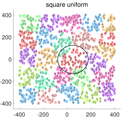
(a)

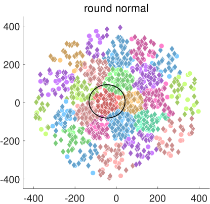
(b)

Figure 1: Illustration of two different scenarios of ultra-dense networks. Each color represents an individual cluster. The brighter dots represent the BSs and the darker diamonds represent the users. We randomly pick one cluster (marked by a black circle) as our focus to analyze the capacity. (a) Square network area with uniformly distributed network nodes. (b) Round network area with truncated normally distributed network nodes.

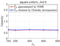
(a)

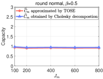
(b)

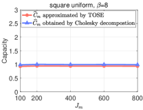
(c)

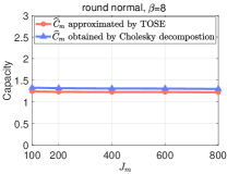
(d)

Figure 2: The comparison of $\widehat{C}_{m}$ obtained by the TOSE algorithm (red lines) and the benchmark algorithm based on Cholesky decomposition (blue lines) under different network settings. (a) and (c): Network nodes are uniformly distributed in a square network area, with $\beta=0.5$ and $\beta=8$, respectively. (b) and (d): Network nodes are truncated normally distributed in a round network area, with $\beta=0.5$ and $\beta=8$, respectively.

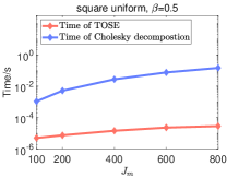
(a)

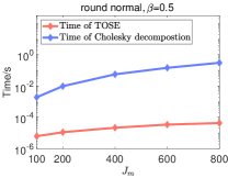
(b)

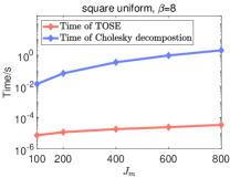
(c)

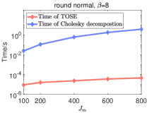
(d)

Figure 3: The comparison of computational time by the TOSE algorithm (red lines) and the benchmark algorithm based on Cholesky decomposition (blue lines) under different network settings. (a) and (c): Network nodes are uniformly distributed in a square network area, with $\beta=0.5$ and $\beta=8$, respectively. (b) and (d): Network nodes are truncated normally distributed in a round network area, with $\beta=0.5$ and $\beta=8$, respectively.

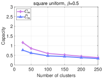
(a)

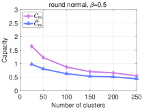
(b)

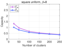
(c)

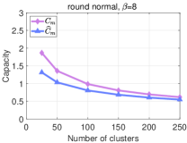
(d)

Figure 4: Comparisons between the theoretical $C_{m}$ (purple lines) and approximated $\widehat{C}_{m}$ (blue lines) under different network settings. (a) and (c): Network nodes are uniformly distributed in a square network area, with $\beta=0.5$ and $\beta=8$, respectively. (b) and (d): Network nodes are truncated normally distributed in a round network area, with $\beta=0.5$ and $\beta=8$, respectively.

TABLE I: The Network Setting

Symbol	Definition	Value
$D$	Network scale	800m
$d_{0}$	Near field threshold	10m
$d_{1}$	Far field threshold	50m
$P$	Transmit power	1W
$N_{0}$	Noise power	$1\times 10^{-12}$ W
$M$	Number of clusters	25
$N/\textrm{rank}(\mathbf{B}_{m})$	Spike ratio	$0.7$
$\beta$	The ratio between the number of users and the number of BSs	0.5, 8

To illustrate the high accuracy of our TOSE algorithm, we compute the values of $\widehat{C}_{m}$ obtained by TOSE and the conventional method based on the Cholesky decomposition, respectively, and plot the results under different scenarios in Fig. 2. Note that we choose the method based on Cholesky decomposition as the baseline to derive the accurate values of $\widehat{C}_{m}$ according to (10), and use our TOSE algorithm to estimate $\widehat{C}_{m}$. It can be observed from Fig. 2 that our TOSE algorithm can accurately estimate $\widehat{C}_{m}$ under different network settings. The estimation errors are indeed less than 5%, which means TOSE is sufficiently accurate in practice.

The computational time of TOSE and the Cholesky decomposition based method are plotted in Fig. 3. By data fitting, we can derive the empirical complexity of TOSE is $O(J_{m})$, while that of the Cholesky decomposition based method is around $O(J_{m}^{3})$. This results indicates the overwhelming superiority in computational cost of TOSE. Combining Fig. 2 and Fig. 3, we can find that TOSE has the same accuracy as the Cholesky decomposition based method, but has much lower computational time.

In Fig. 4, we show the comparisons between the theoretical values of the capacity $C_{m}$ in (7) and the approximation of $\widehat{C}_{m}$ in (10) obtained by TOSE, varying the number of clusters. We set the number of BSs in each cluster around 100, so increasing the number of clusters is equivalent to increasing the density of network nodes, under a fixed network area. It can be observed from Fig. 4 that as the number of clusters increases, the approximated capacity $\widehat{C}_{m}$ gets closer and closer to the theoretical capacity $C_{m}$, which means that our proposed TOSE algorithm has a higher accuracy on the capacity estimation for the ultra-dense networks.

V Conclusion

Capacity is the most important performance metric of wireless networks. Determining the capacity of ultra-dense networks in a fast and accurate way is challenging. In this paper, we propose a TOSE algorithm to estimate the average cluster capacity, which is accurate, fast, and general. Through making use of the spiked model in RMT, we realize a fast approximation of the top $N$ eigenvalues of a large-dimensional random matrix. The capacity can thus be estimated, avoiding the complex steps to calculate the exact eigenvalues. Both analytical and simulated results show that, our TOSE algorithm has a linear time complexity, which is much lower than the polynomial time of exiting eigenvalue-calculation-based methods. Simulation results also show that the accuracy of TOSE is almost the as the exiting eigenvalue calculation based method, on capacity estimation. The estimation error is below 5%. More importantly, TOSE has superior generality, since it is independent of the BS distribution, the user distribution, and the shape of the network area.

References

- [1] W. Xu, G. Zhang, B. Bai, C. Ai, and J. Wu, “Ten key ICT challenges in the post-Shannon era,” Scientia Sinica (Mathematica), vol. 51, no. 7, pp. 1095–1138, 2021.
- [2] C. E. Shannon, “A mathematical theory of communication,” The Bell system technical journal, vol. 27, no. 3, pp. 379–423, 1948.
- [3] T. M. Cover and J. A. Thomas, Elements of Information Theory, 2nd ed. John Wiley & Sons, 2006.
- [4] E. Telatar, “Capacity of multi-antenna Gaussian channels,” European transactions on telecommunications, vol. 10, no. 6, pp. 585–595, 1999.
- [5] E. Björnson and L. Sanguinetti, “Scalable Cell-Free Massive MIMO Systems,” IEEE Transactions on Communications, vol. 68, no. 7, pp. 4247-4261, Jul. 2020.
- [6] G. Interdonato, E. Björnson, H. Q. Ngo, P. Frenger, and E. G. Larsson, “ Ubiquitous cell-free Massive MIMO communications,” EURASIP J. Wireless Commun. Netw, vol. 2019, no. 1, pp. 1–13, Dec. 2019
- [7] M. Matthaiou, O. Yurduseven, H. Q. Ngo, D. Morales-Jimenez, S. L. Cotton and V. F. Fusco, “The Road to 6G: Ten Physical Layer Challenges for Communications Engineers,” IEEE Communications Magazine, vol. 59, no. 1, pp. 64-69, Jan. 2021.
- [8] L. Yang, P. Li, M. Dong, B. Bai, D. Zaporozhets, X. Chen, W. Han, and B. Li, “C2: A Capacity-Centric Architecture Towards Future Wireless Networking,” IEEE Transactions on Wireless Communications, 2022. Doi: 10.1109/TWC.2022.3164286.
- [9] J. Wang, L. Dai, L. Yang, and B. Bai, “Rate-constrained network decomposition for clustered cell-free networking,” in Proc. IEEE ICC 2022.
- [10] C. Deng, L. Yang, H. Wu, D. Zaporozhets, M. Dong, and B. Bai,“CGN: A capacity-guaranteed network architecture for future ultra-dense wireless systems,” in Proc. IEEE ICC 2022.
- [11] A. M. Tulino, S. Verdú. “Random matrix theory and wireless communications,” Foundations and Trends in Communications and Information Theory, vol. 1, no. 1, pp. 1–182, 2004.
- [12] W. H. Press, S. A. Teukolsky, W. T. Vetterling, and B. P. Flannery, Numerical Recipes in C: The Art of Scientific Computing, 2nd ed. Cambridge University Press, 1992.
- [13] J. W. Silverstein,“ Limiting Eigenvalue Behavior of a Class of Large Dimensional Random Matrices Formed From a Hadamard Product”, arXiv: 2112.04617, unpublished.
- [14] R. Kress, Numerical Analysis. Springer, 1998.
- [15] V. A. Marčenko, and L. A. Pastur, “ Distribution for some sets of random matrices,” Math. USSR-Sb., vol. 1, no. 4, pp. 457–483, 1967.
- [16] Z. Bai and J. W. Silverstein, Spectral analysis of large dimensional random matrices. Springer, 2010, vol. 20.
- [17] I. M. Johnstone, “On the distribution of the largest eigenvalue in principal components analysis,” The Annals of Statistics, vol. 29, no. 2, pp. 295-327, 2001.