Estimation of space weathering timescale on (25143) Itokawa: Implications on its rejuvenation process

Abstract

Context. The space weathering timescale of near-Earth S-type asteroids has been investigated by several approaches (i.e., experiments, sample analyses, and theoretical approaches), yet there are orders of magnitude differences.

Aims. We aim to examine the space weathering timescale on a near-Earth S-type asteroid, Itokawa using Hayabusa/AMICA images and further investigate the evolutional process of the asteroid.

Methods. We focused on bright mottles on the boulder surfaces generated via impacts with interplanetary dust particles (IDPs). We compared the bright mottle size distribution with an IDP flux model to determine the space weathering timescale.

Results. As a result, we found that the space weathering timescale on Itokawa’s boulder surfaces is 10${}^{3}$ years (in the range of 10${}^{2}$–10${}^{4}$ years), which is consistent with the timescale of space weathering by light ions from the solar wind.

Conclusions. From this result, we conclude that Itokawa’s surface has been weathered shortly in 10${}^{3}$ years but portions of the surface are exposed via seismic shaking triggered by a recent impact that created the Kamoi crater.

1 Introduction

Space weathering denotes any surface modification processes that may change the optical, physical, chemical, or mineralogical properties of the surface of an airless body (Clark2002). It is caused by the solar wind ion implantation and the micrometeorite bombardment (Pieters2016). The space weathering effect has been observed on lunar rocks, meteorite samples, and asteroids observed by spacecraft and telescopes (Clark2002). Particularly, materials that consist of ordinary chondrites and S-complex asteroids indicate a decrease in albedo (i.e., darkening), reddening of the visible spectrum ($\lesssim 0.7\ \mu$m), and shallowing of $\sim$1 $\mu$m absorption band via the space weathering (Clark2002).

Meanwhile, there is a counter-process against space weathering: rejuvenation or resurfacing, which exposes fresh materials beneath weathered surfaces. Several possible mechanisms for asteroidal resurfacing have been suggested by previous studies. First, tidal interactions with terrestrial planets would trigger resurfacing of the asteroid (Binzel2010). Seismic shaking by non-destructive impacts would induce granular convection that also rejuvenates surfaces (Richardson2005). Moreover, thermal fatigue, which is caused by diurnal temperature variations, would break boulders and cobbles on the surface and result in the exposure of fresh materials (Delbo2014). Furthermore, Yarkovsky-O’Keefe-Radzievskii-Paddack (YORP) effect accelerates the spin rate and would cause mass shedding and global resurfacing (Pravec2007; Graves2018).

An S-type, near-Earth asteroid, (25143) Itokawa, is one of the most evident exhibitions of space weathering and resurfacing phenomena. The unique trait of the asteroid is a large variety of albedos and spectra on its surface, found from the multi-band imaging observation by the Asteroid Multi-band Imaging Camera (AMICA) onboard the Hayabusa spacecraft (Saito2006). Previous studies proved that space weathering is the primary cause of albedo and spectral variation. Hiroi2006 investigated the Near-Infrared Spectrometer (NIRS) data onboard the Hayabusa spacecraft and constructed modeled spectra of Itokawa as a mixture of the spectrum of an LL5 chondrite (Alta’meem) and nanophase iron, taking account of the space weathering. Ishiguro2007 presented a global map of space weathering degrees using AMICA images. More recently, Koga2018 conducted a principal component analysis on multi-band spectra derived from AMICA images and confirmed that the main trend of the spectral variation is consistent with spectral alteration by laboratory simulations of the space weathering. Moreover, weathered rims found from the returned samples are regarded as the most definitive evidence for the occurrence of space weathering on the asteroid surface (Noguchi2014).

It is, however, important to note that the exposure time of the Itokawa’s surface material is not well determined, although the Hayabusa project comprehensively explored the asteroid via remote-sensing observations and laboratory analyses of the returned samples. There is a large discrepancy in the estimate of the surface age up to four orders of magnitude (from 100 years to 10${}^{6}$ years, Bonal2015; Koga2018; Noguchi2011; Keller2014; Matsumoto2018; Nagao2011). In addition, there is still an enormous discrepancy between mechanisms for determining the space weathering timescale of an S-type asteroid. It thus depends on the physical processes that cause the space weathering ($10^{8}$ years for micrometeorite impacts, Sasaki2001; $10^{4}-10^{6}$ years for heavy-ion irradiation, Brunetto2006; $10^{3}-10^{4}$ years for H${}^{+}$ and He${}^{+}$ ion irradiation, Hapke2001 and Loeffler2009). These discrepancies are major obstacles to understanding the evolutional history of Itokawa’s surface.

We propose a novel idea to estimate the Itokawa’s surface age, focusing on bright mottles on the boulder surfaces to alleviate these discrepancies. It was reported that the bright mottles consist of fresh material under the weathered patina of boulders that are exposed by impacts with mm- to cm-sized interplanetary dust particles (IDPs, Takeuchi2009; Takeuchi2010). Because these mottles obscure via space weathering to make them darker and redder again, the number of observable mottles is controlled by the balance of the timescale of space weathering and the IDPs impact frequency. We calculated the occurrence frequency of the bright mottles as a function of size and compared the frequency to the number of the bright mottles to determine the space weathering timescale on Itokawa. Here, we defined the space weathering timescale as the characteristic time needed for changing from fresh ordinary chondrite (OC)-like optical property to the typical (i.e., matured) optical property of the Itokawa surface. We describe our method in Sect. 2 and findings in Sect. 3. Based on these results, we discuss the possible resurfacing mechanism which results in the large-scale optical heterogeneity in Sect. LABEL:sect4.

Table 1: Images used in this study

File name	Filter	Date and Time (UT)	Spacecraft distance (m)	Pixel scale (mm pixel${}^{-1}$)
ST_2544540977	v	2005-11-12 05:35:37	110.9	11.0
ST_2544579522	v	2005-11-12 05:55:52	59.9	5.9
ST_2544617921	v	2005-11-12 06:05:55	77.9	7.7
ST_2563511720	v	2005-11-19 20:23:36	80.9	8.0
ST_2572745988	v	2005-11-19 20:26:36	62.9	6.2

Figure 1: Distance between the spacecraft and the Itokawa’s surface. The grey circles denote the data taken by Hayabusa/LIDAR in 2005 November (Mukai2012). Red (open and filled) circles indicate the distances of the spacecraft when each image was taken at distances closer than 200 m. Filled red circles show the images examined in this study.

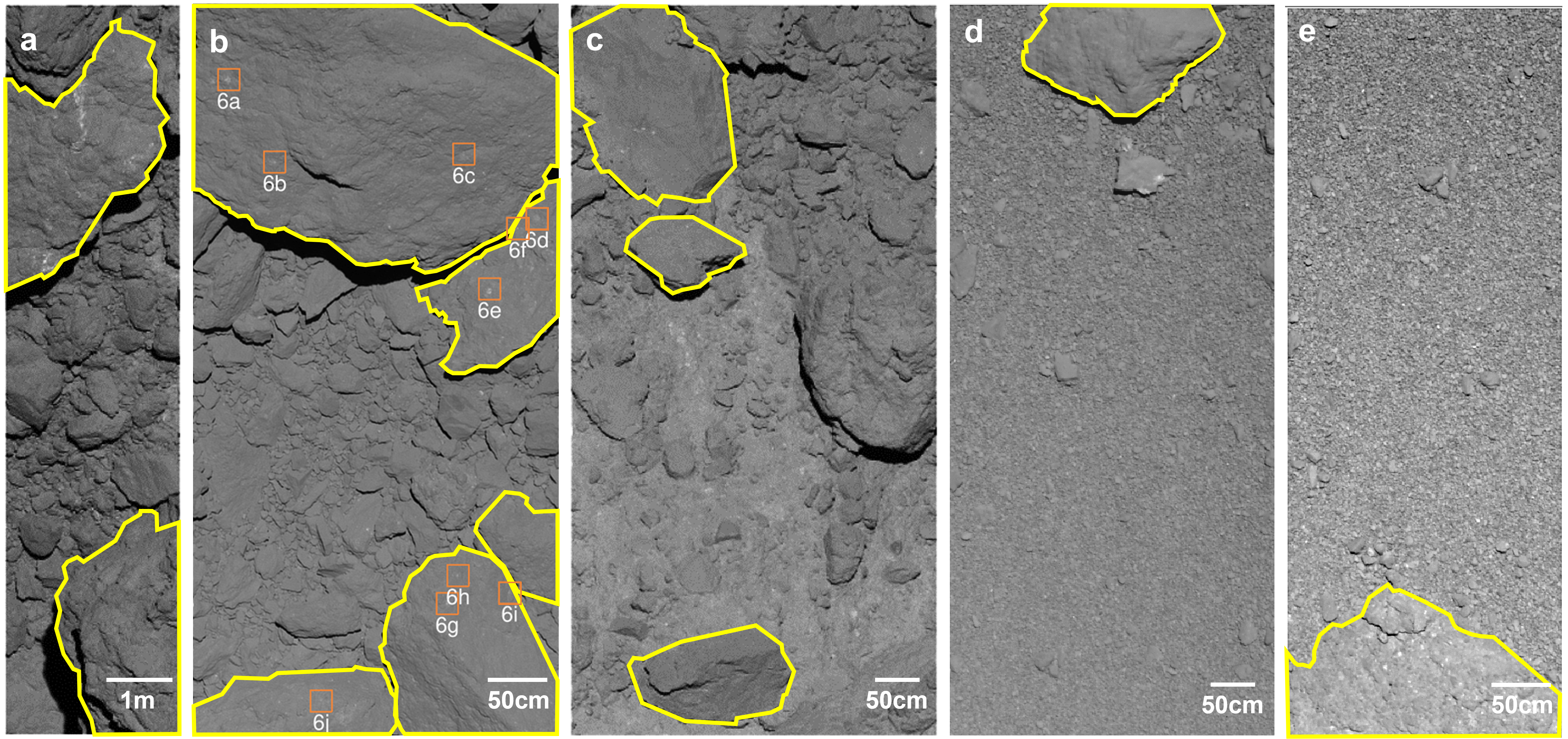
Figure 2: Five images analyzed in this study. The file names are (a) ST_2544540977_v, (b) ST_2544579522_v, (c) ST_2544617921_v, (d) ST_2563511720, and (e) ST_2572745988. We selected twelve large boulders (enclosed by yellow lines) for the analysis. We show enlarged images of the areas surrounded by orange squares in Fig. LABEL:Fig6.

2 Methods

In this chapter, we describe data preparation, the bright mottle detection technique, and a model for comparing our observational results with IDP impact flux, as shown below.

2.1 Data preparation

The Hayabusa spacecraft arrived at the gate position (about the 20 km distance from Itokawa) on 2005 September 12 and shifted to the home position (about the 7 km distance from Itokawa) (Fujiwara2006). During these phases, the mission team investigated the global structures of the asteroid using onboard instruments. In October, the spacecraft moved to several positions with different solar phase angles and approached closer distances for detailed investigations. The mission team conducted two touchdown rehearsals on 2005 November 4 and 12 (Yano2006). Finally, the spacecraft landed on the Itokawa surface on 2005 November 19 (Fujiwara2006). Figure 1 shows the altitudes of the spacecraft in November. This data was taken by Light Detection and Ranging instrument (LIDAR) (AbeS2006; Mukai2007). In Fig. 1, we emphasized the altitude at which the AMICA images were obtained with different symbols (the open and filled red circles).

Among the imaging data available at the official website of Data Archives and Transmission System (DARTS), Institute of Space and Astronautical Science (ISAS), Japan Aerospace Exploration Agency (JAXA) , we selected five AMICA images (ST_2544540977_v, ST_2544579522_v, ST_2544617921_v, ST_2563511720_v, and ST_2572745988_v) taken on 2005 November 12 and 19 (Fig. 2). These images were taken during the second rehearsal and touchdown. We selected these images because they have good spatial resolutions ($<$15 mm pixel${}^{-1}$ ) and contain large boulders (whose longest axis is longer than 1 m). The resolution and boulder sizes are important factors in detecting small mottles and increasing the reliability of the statistical analysis by the law of large population. We did not use ST_2563537820_v (an open circle at November 19 in Fig. 1) for our analysis because there is no large ($>$ 1 m) boulders in the image despite high resolution (6.9 mm pixel${}^{-1}$). Detailed information on the images for our analysis is shown in Table 1.

We subtracted bias and corrected flat from the raw images following Ishiguro2010. After the preprocessing, we applied the Lucy-Richardson deconvolution algorithm to improve the blurred resolution of the AMICA images (Richardson1972; Lucy1974). The usability of the deconvolution technique is confirmed in Ishiguro2010.

2.2 Detection of bright mottles from images

Because small boulders tend to be covered by movable regolith particles, bare rock surfaces may not be exposed on the small boulders. For this reason, we selected a total of 12 large boulders (Fig. 2). These boulders have the longest axis larger than 1 m. Assuming that boulders’ surfaces are perpendicular to the AMICA boresight vector, the total surface area is estimated to be 27.1 m${}^{2}$.

We utilized Source-Extractor, (Bertin1996)) to detect bright mottles from boulders. Note that there is large scale brightness fluctuation on a boulder surface due to the different illumination conditions. This inhomogeneity is not common in astronomical images, for which Source-Extractor is mainly designed. Therefore, we flattened the background by subtracting smoothed images made from a 2-dimensional median filter (without using the background detection algorithm in Source-Extractor). We applied the 2-dimensional median filter with a square width of 19 pixels to the original image. We decided the filter size to flatten the large-scale background ($\gtrsim$10 cm) while leaving small structures of bright mottles ($\lesssim$10 cm). Figure 3 a, b, c are the example of the original, median-filtered, and background-subtracted images of a boulder, respectively.

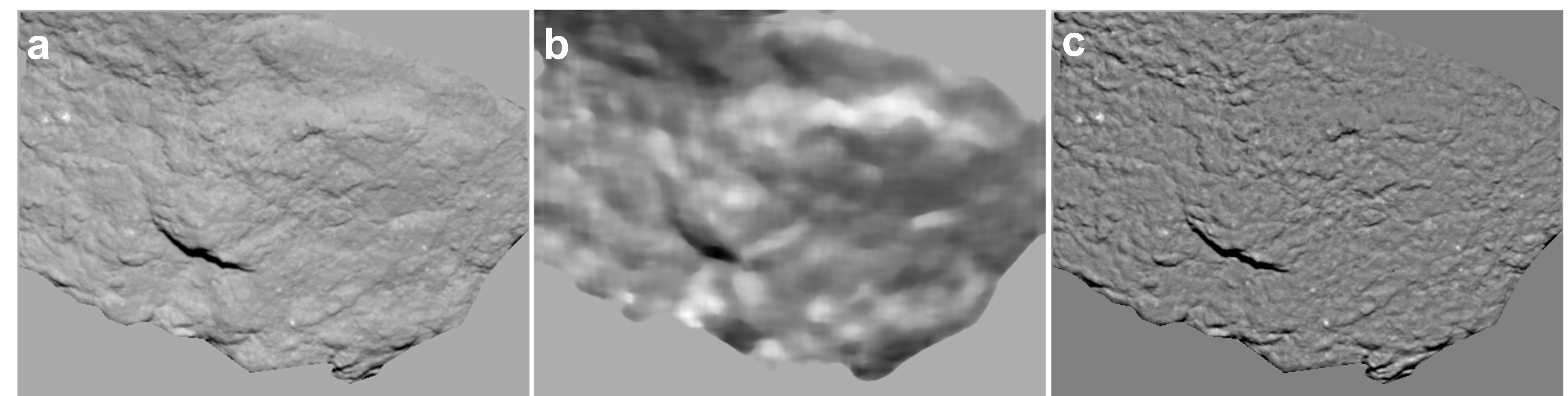
Figure 3: An example of the (a) original, (b) median-filtered, and (c) background-subtracted images used for the analysis. The original image is a part of ST_2544579522_v.fits.

Then, we ran Source-Extractor with a 3-sigma detection threshold. This threshold was chosen to discriminate bright mottles from the small-scale fluctuations caused by the Poisson noise and textures of the boulders. On the other hand, the background mesh size for the calculation of background standard deviation is also 19 pixels, the same size as the median filter. The minimum area for the detection is 2 pixels to avoid false detection due to hot pixels. With this setting, we detected 499 bright sources out of 12 boulders. After this detection process, we rejected sources with elongations (the ratio of major to minor axis) larger than 2.5. This criteria is based on (Elbeshausen2013), which showed the elongation of crater is lower than 2.5 except extreme impact conditions (impact angle ¡ 5 degrees). From this criterion, we filtered out 57 sources (11.4 percent of detected sources) and determined 442 sources as bright mottles created by impacts with interplanetary dust particles.

We counted the number of pixels above the threshold for each bright mottle and calculated the area covered by these pixels. After that, we converted the area to the diameter of a circle with an equivalent area. Hereafter, we refer to this diameter as the size of the bright mottle. Once we obtained the size, we derived cumulative size-frequency distributions (SFDs) of bright mottles on ten boulders. We employed a logarithmic bin size (Crater1979). The range and bin size of the crater’s SFDs are given in Table 2.

Table 2: Notations and ranges of discrete values for impactor’s mass, velocity, mass density, and crater diameter used in Sect. 2.3

	Mean${}^{(a)}$	Notation${}^{b)}$	Min${}^{(c)}$	Max${}^{(d)}$	Width${}^{(e)}$	Num${}^{(f)}$
Crater diameter (mm)	$\bar{D}$	$D_{l}$	2.6	2.6$\times$10${}^{4}$	2${}^{0.25}D_{l,\textrm{min}}$	50
Impactor mass (g)	$\bar{m}$	$m_{i}$	1.1$\times$10${}^{-6}$	8.9	10${}^{0.1}m_{i,\textrm{min}}$	69
Impactor velocity (km s${}^{-1}$)	$\bar{v}$	$v_{j}$	0.5	89.5	1.0	90
Impactor mass density (g cm${}^{-3}$)	$\bar{\delta}$	$\delta_{k}$	0.125	7.975	0.05	158

2.3 IDP impact model

As described above, we consider that recent IDP impacts on the bare boulder surface formed bright mottles. Accordingly, if the IDP impact flux is known, it is possible to derive the number of mottles and compare it to the numbers of the detected bright mottles. We utilized the Meteoroid Engineering Model Version 3 (MEM3, Moorhead2020) model to derive the IDPs impact flux colliding with boulder surfaces. This model was developed for the risk assessment of spacecraft navigating in the near-Earth region (the heliocentric distance between 0.2 au and 2.0 au). It is also applicable to any celestial bodies if the orbital information is given. We obtained Itokawa’s orbital information from the JPL Horizons Web interface . This ephemeris includes state vectors of Itokawa with respect to Earth, starting from 2019 June 10 (JD 2 458 644.5) to 2020 December 16 (JD 2 459 199.5) for 555 days (approximately one orbital period of Itokawa, Fujiwara2006). We assumed that the flux averaged over 1 orbital period remained as a constant since the orbit of the asteroid has not been significantly altered during 1 Million years (2002ESASP.500..331Y). Because the rotation axis of Itokawa is nearly aligned to the ecliptic south pole ([$\lambda,\beta$]=[128$\aas@@fstack{\circ}$5, -89$\aas@@fstack{\circ}$66], where $\lambda$ and $\beta$ are ecliptic longitude and latitude of the pole orientation, Demura2006 and Fujiwara2006), in addition, the boulders for our analysis distribute near the equatorial region, we employed azimuthally-averaged flux. It is the impact flux to a target body rotating around the ecliptic pole and averaged along the azimuth direction.

The MEM3 model assumes two meteoroid populations, namely, high and low-density populations with different mass densities based on Kikwaya2011. For each population, the MEM3 model calculates the impact flux per square meter per year, $H(v)$, as a function of the impactor’s velocity $v$ in the mass range of $m_{\mathrm{min}}\leqq m\leqq m_{\mathrm{max}}$, where $m_{\mathrm{min}}=10^{-6}$ g and $m_{\mathrm{max}}=10$ g are given, respectively. In Fig. 4, we show $H(v)$ for a target in the Itokawa’s orbit, where we specified the velocity interval of $\Delta v=1$ km s${}^{-1}$ for the calculation.

$H(v)$ is written as

$$H(v)=\int_{m_{\mathrm{min}}}^{m_{\mathrm{max}}}f(m,v)\,dm\leavevmode\nobreak\ ,$$ (1)

where $f(m,v)$ is a differential impact flux distribution with respect to $v$ and $m$, per square meter per year. It is important to note that the mass dependency of the impact flux is not available in $H(v)$ because it has an integrated form with respect to $m$. Accordingly, $f(m,v)$ in Eq. (1) is more useful than $H(v)$ for our study because we need to compare the size (derivable from $m$) frequency distribution of the bright mottles with a model. Following the recommendation in Moorhead2020, we incorporated the cumulative IDPs flux model $F_{\textrm{Gr\"{u}n}}(m)$ in Gruen1985 into $H(v)$ obtained by the MEM3 model. It is given by

$$F_{\textrm{Gr\"{u}n}}\left(m\right)=\left(c_{1}m^{\gamma_{1}}+c_{2}\right)^{\gamma_{2}}+c_{3}\left(m+c_{4}m^{2}+c_{5}m^{4}\right)^{\gamma_{3}}+c_{6}\left(m+c_{7}m^{2}\right)^{\gamma_{4}}\leavevmode\nobreak\ ,$$ (2)

where $c_{1}=2.2\times 10^{3}$, $c_{2}=15$, $c_{3}=1.3\times 10^{-9}$, $c_{4}=10^{11}$, $c_{5}=10^{27}$, $c_{6}=1.3\times 10^{-16}$, $c_{7}=1.0\times 10^{6}$, $\gamma_{1}=0.306$, $\gamma_{2}=-4.38$, $\gamma_{3}=-0.36$, and $\gamma_{4}=-0.85$ are constants. The mass, $m$, is in the unit of a gram in Eq. (2).

With $F_{\textrm{Gr\"{u}n}}(m)$, the cumulative IDP flux with the particle mass larger than $m$ is given as a function of mass and velocity:

$$F(m,v)=H(v)\frac{F_{\textrm{Gr\"{u}n}}(m)}{F_{\textrm{Gr\"{u}n}}(m_{\mathrm{min}})}\leavevmode\nobreak\ ,$$ (3)

where we chose the denominator (the cumulative flux for $m>m_{\mathrm{min}}$) to conserve the total flux. Because the MEM3 model generates the flux for discrete velocity and mass density (see below) values, we hereafter notate discrete values as $(m_{i},v_{j},\delta_{k})$ rather than $(m,v,\delta)$ for mass, velocity, and mass density. Table 2 summarizes the notation and the range of these discrete physical quantities. For our convenience, we converted the cumulative flux $F_{\textrm{Gr\"{u}n}}(m_{i})$ into the differential flux within i-th mass bin as below:

$$\begin{split}f(m_{i},v_{j})&=F(m_{i},v_{j})-F(m_{i+1},v_{j})\\ &=\frac{F(m_{\mathrm{min}},v_{j})}{F_{\textrm{Gr\"{u}n}}(m_{\mathrm{min}})}\Bigl{(}F_{\textrm{Gr\"{u}n}}\left(m_{i}\right)-F_{\textrm{Gr\"{u}n}}\left(m_{i+1}\right)\Bigr{)}\leavevmode\nobreak\ .\\ \end{split}$$ (4)

The MEM3 model also provides a probability distribution of the mass density $\delta_{k}$. The probability distribution function, $C(\delta_{k})$, is defined as the ratio of the number of particles within a given density bin to the total number of particles. In the MEM3 model, $C(\delta_{k})$ is independent of $m_{i}$ and $v_{j}$. With this function, the IDP flux for a given mass, velocity, and mass density is calculated from

$$f^{\prime}(m_{i},v_{j},\delta_{k})=f(m_{i},v_{j})\leavevmode\nobreak\ C(\delta_{k})\leavevmode\nobreak\ .$$ (5)

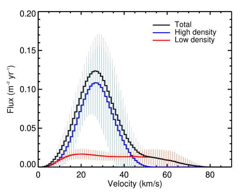
Figure 4: Cumulative IDPs flux averaged over Itokawa’s one orbital revolution around the Sun. The error bars correspond to the range of the IDP flux during the one orbit revolution.

Next, we considered the crater size generated by an IDP impact with a given $m_{i}$, $v_{j}$, and $\delta_{k}$. We utilized the crater size model in Holsapple1993. We thus calculated the cratering volume $V(\bar{m}_{i},\bar{v}_{j},\bar{\delta}_{k})$ excavated by an impact with given mean mass $\bar{m}_{i}$ ($:=(m_{i}+m_{i+1})/2$), mean velocity $\bar{v}_{j}$ ($:=(v_{j}+v_{j+1})/2$), and mass density $\bar{\delta}_{k}$ ($:=(\delta_{k}+\delta_{k+1}/2$) by following equations

$$\pi_{V}=K_{1}\left(\pi_{2}\pi_{4}^{\frac{6\nu-2-\mu}{3\mu}}+\left(K_{2}\pi_{3}\pi_{4}^{\frac{6\nu-2}{3\mu}}\right)^{\frac{2+\mu}{2}}\right)^{\frac{-3\mu}{2+\mu}}\leavevmode\nobreak\ ,$$ (6)

$$\pi_{V}=\frac{\rho V}{\bar{m_{i}}}\,,\;\pi_{2}=\frac{g\bar{a}_{i,k}}{\bar{U_{j}}^{2}}\,,\;\pi_{3}=\frac{Y}{\rho\bar{U_{j}}^{2}}\,,\;\pi_{4}=\frac{\rho}{\bar{\delta}_{k}}\leavevmode\nobreak\ ,$$

where $\pi_{V}$ is the so-called cratering efficiency, defined as a ratio of the crater mass to the impactor mass (Holsapple1993). $\bar{a}_{i,k}$ and $\bar{U}_{j}$ denote the mean radius and the normal component of the mean velocity of the impactor, respectively. We assumed an oblique impact with the most probable impact angle $\theta=45\degr$ (Gault1978). This assumption of the oblique impact reduces the vertical impact velocity by a factor of $\sqrt{2}$ (i.e., $\bar{U}=\bar{v}/\sqrt{2}$). The constants, $Y$, $\rho$, and $g$ are the tensile strength, the bulk density, and the surface gravity of the target body. We assumed a spherical impactor whose mean radius is given as below

$$\bar{a}_{i,k}=\left(\frac{3}{4\pi}\frac{\bar{m}_{i}}{\bar{\delta}_{k}}\right)^{1/3}\leavevmode\nobreak\ .$$ (7)

To obtain the crater volume $V(\bar{m}_{i},\bar{v}_{j},\bar{\delta}_{k})$, we used Eq. (6)–(7) for impactors with given $\bar{m}_{i}$, $\bar{v}_{j}$, and $\bar{\delta}_{k}$. We substituted $\rho=3.4$ g cm${}^{-3}$ based on the measurement of the bulk density of Itokawa’s samples (Tsuchiyama2011). The gravitational acceleration on the Itokawa surface is given as $g=8.4\times 10^{-3}$ cm s${}^{-2}$ (Tancredi2015). For the other parameters for characterizing the target boulders, we assumed a hard rock-type material and referred to the values in (Holsapple1993; Holsapple2022). Table 3 summarizes the applied values for the computation. With Eq. (6), we calculated $\pi_{V}$ for each impactor with given $\bar{m}_{i}$, $\bar{v}_{j}$, and $\bar{\delta}_{k}$, and obtained the crater mass $\rho V$. The crater radii were then derived as $R=K_{r}V^{1/3}$, in the case of a simple bowl-shaped crater (Holsapple2022).

Table 3: Parameters used for the evaluation of the crater’s diameter

Parameter	Applied value	Reference
$K_{1}$	0.06	1
$K_{2}$	1	1
$\nu$	0.33	1
$\mu$	0.55	2
$\rho$	3.4 (g cm${}^{-3}$)	3
$g$	$8.4\times 10^{-3}$ (cm s${}^{-2}$)	4
$Y$	$1.44\times 10^{8}$ (g cm s${}^{-2}$)	1
$K_{r}$	1.1	1

(1) Holsapple2022; (2) Holsapple1993; (3) Tsuchiyama2011; (4) Tancredi2015

Holsapple2013 asserted that craters on small (sub-km sized) asteroids are expected to be spall craters. They are a kind of craters surrounded by shallow spallation features with diameters larger than 2–4 times of those of simple bowl-shaped craters. Since the depth of the space weathered rim layer found in Itokawa samples is thin enough ($<1\mu$m, Noguchi2014), it is reasonable to assume that the diameters of bright mottles are equivalent to the diameter of the bowl-shaped craters. Therefore, the diameter of bright mottles including spalled region can be given as $D=2C_{\mathrm{spall}}R$ $(2\leq C_{\mathrm{spall}}\leq 4)$. We will discuss the effect of $C_{\mathrm{spall}}$ in Sect. LABEL:sect4_2_5.

After deriving $D$, we counted the total number of the craters within given diameter bins, $N(D_{l})$. For the consideration of the diameter bins, we employed a logarithmic bin size to match the bright mottle SFD from the observation, namely,

$$D_{l}=2^{\frac{l}{4}-1}\leavevmode\nobreak\ \leavevmode\nobreak\ \leavevmode\nobreak\ (l=1,2,\dots 50)\leavevmode\nobreak\ .$$ (8)

Then, the number of craters within l-th diameter bin, $N(D_{l})$ is counted as

$$\begin{array}{ccc}\hfill N(D{}_l)& =\sum {}_{l=1}{}^{50}cf{}^{\prime }(\overline{m}{}_i,\overline{v}{}_j,\overline{\delta }{}_k)\{\begin{array}{cc}c\hfill & \end{array}=1,\hfill & \hfill \text{if }D{}_l\le D(\overline{m}{}_i,\overline{v}{}_j,\overline{\delta }{}_k)\le D{}_{l+1}\\ \hfill c=0,& \text{otherwise},\hfill \end{array}wherethesubscript\text{l}isanordinalnumberupto50(i.e.,\text{l=1,2, …, 50}).\text{33§33Results}Weidentified442brightmottlesfromtwelveboulders(theprojectedtotalareaof27.1m\text{^2}).Theaveragespatialdensityis16.3m\text{^-2}.Hereafter,weshowourfindingsasbelow.\text{3.13.1§3.13.1Cumulat}$$ (10)