MIME: Minority Inclusion for Majority Group Enhancement of AI Performance

Abstract

Several papers have rightly included minority groups in artificial intelligence (AI) training data to improve test inference for minority groups and/or society-at-large. A society-at-large consists of both minority and majority stakeholders. A common misconception is that minority inclusion does not increase performance for majority groups alone. In this paper, we make the surprising finding that including minority samples can improve test error for the majority group. In other words, minority group inclusion leads to majority group enhancements (MIME) in performance. A theoretical existence proof of the MIME effect is presented and found to be consistent with experimental results on six different datasets. Project webpage: https://visual.ee.ucla.edu/mime.htm/.

1 Introduction

Inclusion of minorities in a dataset impacts the performance of artificial intelligence (AI). Recent research has presented the value of inclusive datasets to improve AI performance on minorities and also for society-at-large [21, 11, 34, 44, 35, 37, 29, 23, 30]. A society-at-large consists of both majority and minority stakeholders. However, an objection (often silently posed) to minority inclusion efforts, is that the inclusion of minorities can diminish performance for the majority. This is based on a “rule of thumb” that AI performance is maximized when one trains and tests on the same distribution. A devil’s advocate position against minority inclusion might be presented as: “In a fictitious society where we are absolutely certain that only blue-skinned humans will exist in the test set, why include out of distribution orange-skinned humans in the training set?”.

In this paper, we make the surprising finding that inclusion of minority samples improves AI performance not just for minorities, not just for society-at-large, but even for majorities. We refer to this effect as Minority Inclusion, Majority Enhancement (MIME), illustrated in Figure 2. Specifically, we note that including some minority samples in the train set improves majority group test performance. However, continued addition of minority samples leads to performance drop. The effect holds under statistical conditions that are represented in traditional computer vision datasets including FairFace [32], UTKFace [56], pets [22], medical imaging datasets [40] and even non-vision data [9]. Although deep learning is used for these problems, the flattening layer of a network can be empirically approximated to elementary distributions like Gaussian Mixture Models (GMMs). A GMM facilitates closed-form analysis to prove the existence of the MIME effect. Additionally, we show existence of MIME on general distributions. Classification experiments on neural networks validate using Gaussian mixtures: complex neural networks exhibit feature embeddings in flat layers, distributed with approximately Gaussian density, across six datasets, in and beyond computer vision, and across many realizations and configurations.

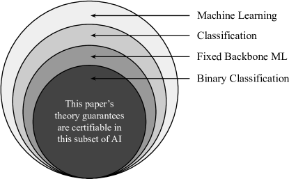
Figure 1: This paper proves* that including minorities improves majority performance. *When do the provable guarantees hold? The guarantees are certifiable for fixed backbone binary classification (e.g. one uses a head network with pretrained weights and fine-tunes a downstream layer for classification). The fixed backbone ML is far from a toy scenario (it is considered SoTA by some authors [31]) and also enables provable certification - ordinarily it is hard to prove things for neural network settings.

Fairness in machine learning is an exceedingly popular area, and our results benefit from several key papers published in recent years. Sample reweighting approaches recognize the need to preferentially weight difficult examples [18, 43, 14]. Active and online learning benefit from insights into sample “informativeness” (i.e. given a budget on the number of training samples, which would be the best sample to include [13, 16]). Domain randomization literature indicates that surprising perturbations to the training set can improve generalization performance [47, 54, 27]. We extend some of these theoretical insights to the sphere of analyzing benefits of minority inclusion on majority performance.

1.1 Contributions

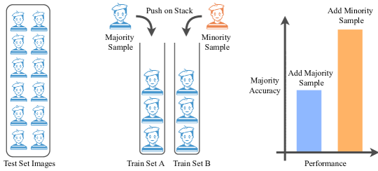
Figure 2: Inclusion of minorities can improve performance for majorities. We theoretically describe an effect called Minority Inclusion, Majority Enhancement (MIME). The figure depicts test classification of blue mimes, and an initial training stack, also of blue mimes. If allowed to add one more training sample, it can be better to push an orange mime onto the training stack rather than a blue mime. Test accuracy can increase by pushing orange, even though the test set consists of blue mimes alone.

While some works [24, 34] have observed related phenomena for isolated tasks, to the best of our knowledge, characterizing benefits to majority groups by including minority data is largely unexplored theoretically. Our contributions are as follows:

• We introduce the Minority Inclusion Majority Enhancement (MIME) effect in a theoretical and empirical setting.

• Theoretically: we derive in closed form, the existence of the MIME effect both with and without domain gap (Key Results 1 and 2) and for general sample distributions (Key Result 3).

• Empirically: we test the MIME effect on six datasets, as varied as animals to medical images, and observe the existence of MIME consistent with theory.

1.2 Outline of Theoretical Scope

Figure 1 describes the theoretical scope. Through three key results (Theorem 1, Theorem 2 and Theorem 3), this paper offers an existence proof of the MIME effect. An existence proof can leverage a tractable setting. As in Figure 2, training data is a stack of $K-1$ majority samples. Test data is all majority samples. We can push one additional training sample to increase the stack size to $K$. We are allowed the choice of having the $K$-th sample drawn from the minority or majority group. Theorem 1 proves that, under the assumptions in Section 3, pushing a minority sample is superior for majority group performance improvements. Theorem 2 generalizes this result to a more realistic scenario, with domain gap. Theorem 3 extends the existence proof to general sample distributions. Empirical results on real-world AI tasks offer validation for theoretical assumptions.

2 Related Work

Debiasing and fairness: It has been widely reported that biases in training data lead to biased algorithmic performance [10, 26, 11]. Work has been carried out in identifying and quantifying biases [2, 4, 49] and a range of methods exist to address them [23, 37]. Early approaches suggest oversampling strategies [19, 8]. Other methods propose resampling based on individual performance [35]. Some works utilize information bottlenecks to disentangle biased attributes [46]. Still other methods propose bias mitigation solutions based on adversarial learning [55] or include considerations like protected class-specific classifiers [50]. Generative models have also found use in creating synthetic datasets with debiased attributes [41]. Xu et al. [52] identify inherent bias amplification as a result of adversarial training and propose a framework to mitigate these biases. Our goals are different – while these aim to reduce test time performance bias across groups, we analyze influence of minority samples on majority group performance.

Learning from multiple domains: Domain adaptation literature explores learning from multiple sources [42]. It could therefore be one potential way to analyze our problem of training on combinations of majority and minority data. In our setting, data arising from distinct domains is seen as being drawn from different distributions with a domain gap [6]. Between these domains, [5] establishes error bounds for learning from combinations of domains. However, these error estimates and bounds do not take into account the notion of majority and minority groups; therefore, describing the MIME effect is outside their scope.

Dataset diversity: An important push towards fairness is through analysis of dataset composition. Several works indicate the importance of diverse datasets [21, 29]. Ryu et al. [44] note that class imbalance in the training set leads to performance reduction. Wang et al. [49] highlight that perfectly balanced datasets may still not lead to balanced performance. For designing medical devices, [30] emphasizes the importance of diverse datasets. Through experiments on X-ray datasets, [34] observe that imbalanced training sets adversely affect performance on the disadvantaged group. They also observe that an unbiased training set shows the best overall accuracy. However, their inferences are related empirical observations on a few medical tasks and datasets. From an application perspective, the task of remote photoplethysmography enables analysis of the bias problem. Prior work notes that camera-based heart rate estimation exhibits skin tone bias [39], and [1, 51] propose synthetic augmentations to mitigate this. Additionally, [12, 48] establish that camera based heart rate estimation is fundamentally biased against dark skin tone subjects, establishing a notion of task complexity. While all these works recognize that data composition affects bias, none to our knowledge describe the effect of varying minority group proportions on majority group accuracy.

3 Statistical Origins of the MIME Effect

For more concise exposition, we make assumptions in the main paper derivation and defer extended generality to the supplement. Assumptions include:

• Assumption 1: one-dimensional data samples and binary labels, $x\in\mathbb{R}$, $y\in\{1,2\}$. This is relevant to modern classification problems since the final classification decision is based on a one dimensional projection of the feature representation of the sample with respect to the learnt hyperplane (discussed in Figure 1, Section 4). Additionally, existence proof of MIME holds for more general vectorized notation, as discussed in the supplement.

• Assumption 2: the binary classifier used is a perceptron: this assumption relates to real neural networks since the last layer is perceptron-like [38].

We now introduce some key definitions that follow from these assumptions.
Definition 1: (Task complexity): For binary classification we define task complexity for a group of data $\theta$ as a continuous variable in $[0,1]$, such that,

$$\theta=\underset{h\in H}{\arg\min}\,\,\epsilon(h),$$ (1)

where $\epsilon(h)$ is the classification error for hypothesis $h$ (the classifier), $H$ is the space of feasible hypotheses. It is noted later that this is empirically equivalent to distributional overlap. This definition is not new. Hard-sample mining [18] establishes the of use performance measures as an indicator of difficulty.
Definition 2: (Majority Group): Group class (i.e. group label $g=\textrm{major}$) on which the task performs better. Quantified by training a network only with majority group data and evaluating test performance: $\theta^{\textrm{major}}=\underset{h\in H}{\arg\min}\,\,\epsilon^{\textrm{major}}(h)$.
Definition 3: (Minority Group): Group class (i.e. group label $g=\textrm{minor}$) on which the task performs worse. Quantified by training a network only with minority class data and evaluating test performance: $\theta^{\textrm{minor}}=\underset{h\in H}{\arg\min}\,\,\epsilon^{\textrm{minor}}(h)$.
Definition 4: (Minority Training Ratio ($\beta$)): Ratio of minority to majority samples in the data under consideration (training set, in the context of this paper).
Definition 5: (MIME Domain Gap): Measure of how classification differs for minorities and majorities. Quantified as a difference between ideal hyperplanes. Note that this definition for domain gap could be different from other definitions. In this work, domain gap should be taken to mean MIME domain gap.
Empirical observations on cutting-edge machine learning tasks demonstrate the real-world applicability of the assumptions above. We now discuss three key results. For ease of understanding, we make two simplifying assumptions for Key Results 1 and 2: (i) simplified distributions that follow a symmetric Gaussian Mixture Model, and (ii) equally likely class labels, i.e. $Pr(y=1)=Pr(y=2)$. These assumptions are relaxed in Key Result 3.

Key Result 1: A minority sample can be more valuable for majority classifiers than another majority sample

Our first key result shows that it can benefit performance on the majority group more if one adds minority data (instead of majority data). Consider a binary classification setting with data samples $x\in\mathbb{R}$ and labels $y\in\{1,2\}$. Samples from the two classes are drawn from distributions with distinct means:

$$\begin{split}x&\lvert y=1\sim p_{1}(x\lvert\mu_{1},\sigma_{1})\\ x&\lvert y=2\sim p_{2}(x\lvert\mu_{2},\sigma_{2}).\end{split}$$ (2)

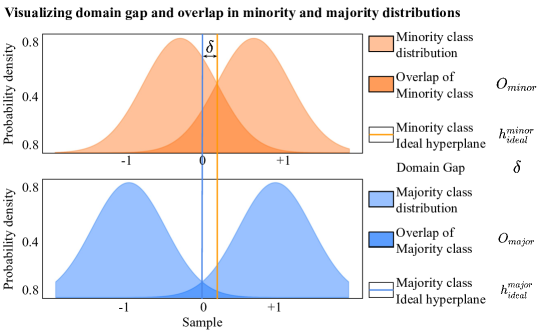
Figure 3: Visualizating of Gaussian Mixture Model parameters. We plot GMMs with different task complexities. The domain gap $\delta$ is visualized as the difference in the ideal threshold locations. The overlap/task complexity metric can be visually seen.

Maximum likelihood (ML) can be used to estimate the label as

$$\widehat{y}=\underset{y}{\arg\max}\,\,\mathcal{L}(x\lvert y).$$ (3)

An ideal hyperplane for ML $\mathcal{H}_{\textrm{ideal}}$ is a set of data samples such that:

$$\mathcal{H}_{\textrm{ideal}}=\big{\{}x\,\,\big{\lvert}\,\,\mathcal{L}(x\lvert y=1)=\mathcal{L}(x\lvert y=2)\big{\}}.$$ (4)

We consider the hyperplane’s geometry to be linear in this one dimensional setting. Therefore the hyperplane can be represented as a normal vector: $\mathbf{h}_{\textrm{ideal}}$. The normalized hyperplane is represented by a two dimensional vector, $\mathbf{h}=[1\,\,b]^{T}$. Here, $b$ is the offset/bias. In general, a hyperplane $\mathbf{h}$ may not be ideal. The accuracy of a hyperplane is based on a performance measure $\mathcal{P}\big{\{}\mathbf{h}\big{\}}$, where the operator $\mathcal{P}$ takes as input the hyperplane and outputs the closeness to the ideal hyperplane $\mathbf{h}_{\textrm{ideal}}$. A goal of a learning based classifier is to obtain:

$$\widehat{\mathbf{h}}=\underset{\mathbf{h}}{\arg\min}\,\,\mathcal{P}\big{\{}\mathbf{h}\big{\}}=\underset{\mathbf{h}}{\arg\min}\,\,\lVert\mathbf{h}-\mathbf{h}_{\textrm{ideal}}\lVert,$$ (5)

where $\widehat{\mathbf{h}}$ is the best learnt estimate of the ideal hyperplane. The ideal hyperplane is the global minimizer of this objective. Now, assume we are provided a finite training set of labelled data $\mathcal{D}_{K-1}=\left\{\left(x_{i},y_{i}\right)\right\}^{K-1}_{i=1}$. Let the estimated hyperplane be $\mathbf{h}_{K-1}$, denoting that $K-1$ samples have been used to learn the hyperplane. If one additional data sample is made available, then the learnt hyperplane would be $\mathbf{h}_{K}$. From Equation 2, the $k$-th sample is drawn from one of two distributions:

$$\begin{split}x_{k}&\lvert y=1\sim p_{1}(x\lvert\mu_{1},\sigma_{1})\\ x_{k}&\lvert y=2\sim p_{2}(x\lvert\mu_{2},\sigma_{2}).\end{split}$$ (6)

We now introduce the notion of majority and minority sampling.

Introducing Majority/Minority Distributions: Suppose that the $k$-th data sample could be drawn for the same classification task from a minority or majority group. Let $g\in\{\textrm{major},\textrm{minor}\}$ denote the group label (for the group class). Equation 2 can now be conditioned on the group label, such that there are four possible distributions from which the $k$-th sample can be drawn:

$$\begin{split}&\left.\begin{array}[]{ll}x_{k}\lvert g=\textrm{major},y=1\sim p^{\textrm{major}}_{1}(x\lvert\mu^{\textrm{major}}_{1},\sigma^{\textrm{major}}_{1})\\ x_{k}\lvert g=\textrm{major},y=2\sim p^{\textrm{major}}_{2}(x\lvert\mu^{\textrm{major}}_{2},\sigma^{\textrm{major}}_{2})\end{array}\right\}\begin{tabular}[c]{@{}c@{}}Majority\\ group\end{tabular}\\ \\ &\left.\begin{array}[]{ll}x_{k}\lvert g=\textrm{minor},y=1\sim p^{\textrm{minor}}_{1}(x\lvert\mu^{\textrm{minor}}_{1},\sigma^{\textrm{minor}}_{1})\\ x_{k}\lvert g=\textrm{minor},y=2\sim p^{\textrm{minor}}_{2}(x\lvert\mu^{\textrm{minor}}_{2},\sigma^{\textrm{minor}}_{2})\end{array}\right\}\begin{tabular}[c]{@{}c@{}}Minority\\ group\end{tabular}\\ \end{split}$$ (7)

Overlap: Let the ideal decision hyperplane be located at $x=d_{\textrm{ideal}}$. Then, given equal likelihood of the two labels for $y$, the overlap for the majority group is defined as the probability of erroneous sample classification:

$$O_{\textrm{major}}=0.5\int^{d_{\textrm{ideal}}}_{x=-\infty}p^{\textrm{major}}_{2}(x)dx+0.5\int^{\infty}_{x=d_{\textrm{ideal}}}p^{\textrm{major}}_{1}(x)dx.$$ (8)

The same definition holds true for the minority class as well. Therefore, by definition, $O_{\textrm{major}}<O_{\textrm{minor}}$. The task complexities $\theta^{\textrm{major}}$ and $\theta^{\textrm{minor}}$ are empirical estimates of the respective overlaps. Hereafter, we assume that all four marginal distributions are Gaussian and symmetric (this is relaxed later for Key Result 3). Figure 3 visually highlights relevant parameters. $O_{\textrm{minor}}>O_{\textrm{major}}$ occurs through the interplay of component means and variances.

The expectation over the class label yields majority and minority sampling:

$$\begin{split}x_{k}^{\textrm{major}}\triangleq x_{k}&\lvert g=\textrm{major}\sim\mathbb{E}_{y}\big{[}x_{k}\lvert g=\textrm{major},y\big{]}\\ x_{k}^{\textrm{minor}}\triangleq x_{k}&\lvert g=\textrm{minor}\sim\mathbb{E}_{y}\big{[}x_{k}\lvert g=\textrm{minor},y\big{]},\\ \end{split}$$ (9)

where we have defined $x_{k}^{\textrm{major}}$ or $x_{k}^{\textrm{minor}}$ as having the $k$-th sample come from the majority or minority distributions.

Armed with an expression for the $k$-th sample, we can consider a scope similar to active/online learning [20, 28, 45, 33, 17, 7, 16, 3]. Suppose a dataset of $K-1$ samples has been collected on majority samples, such that there exists a dataset stack $\mathcal{D}^{\textrm{major}}_{K-1}=\left\{(x_{i}^{\textrm{major}},y^{\textrm{major}}_{i})\right\}^{K-1}_{i=1}$. A hyperplane $\mathbf{h}_{K-1}$ is learnt on this dataset and can be improved by expanding the dataset size. Consider pushing sample index $K$, denoted as $x_{K}$ onto the stack. Now we have a choice of pushing $x_{K}^{\textrm{major}}$ or $x_{K}^{\textrm{minor}}$, to create one of two datasets:

$$\begin{split}\mathcal{D}_{K}^{+}&=\{\mathcal{D}_{K-1}^{\textrm{major}},x_{K}^{\textrm{major}}\}\\ \mathcal{D}_{K}^{-}&=\{\mathcal{D}_{K-1}^{\textrm{major}},x_{K}^{\textrm{minor}}\},\end{split}$$ (10)

where $\mathcal{D}_{K}^{-}$ represents the interesting case where we choose to push a minority sample onto a dataset with all majority samples (e.g. adding a dark skinned sample to a light skinned dataset). Denote $\mathbf{h}^{+}_{K}$ and $\mathbf{h}^{-}_{K}$ as hyperplanes learnt on $\mathcal{D}_{K}^{+}$ and $\mathcal{D}_{K}^{-}$. We now arrive at the following result.

Theorem 1: Let $\mathcal{P}^{\textrm{major}}\big{\{}\cdot\big{\}}$ be the performance of a hyperplane on the majority group. Let $\Delta=\mathcal{P}^{\textrm{major}}\big{\{}\mathbf{h}_{K-1}\}$. Assume that the minority group distribution has an overlap $O_{\textrm{minor}}$ while the majority group has an overlap $O_{\textrm{major}}<O_{\textrm{minor}}$. Both have the same ideal hyperplane $\mathbf{h}_{\textrm{ideal}}$. Under the definitions of $\mathbf{h}^{-}_{K}$ and $\mathbf{h}^{+}_{K}$ as above, assuming $\Delta$ is sufficiently small and the group class distribution variances are not very large,

$$\underset{x_{K}^{\textrm{minor}}}{\mathbb{E}}\mathcal{P}^{\textrm{major}}\big{\{}\mathbf{h}^{-}_{K}\big{\}}<\underset{x_{K}^{\textrm{major}}}{\mathbb{E}}\mathcal{P}^{\textrm{major}}\big{\{}\mathbf{h}^{+}_{K}\big{\}},$$ (11)

stating that, perhaps surprisingly, expected performance for majorities improves more by pushing a minority sample on the stack, rather than a majority sample.
Proof (Sketch): A sketch is provided, please see the supplement for the full proof. The general idea is to show that samples closer to $\mathbf{h}_{\textrm{ideal}}$ are more beneficial, and minority distributions may sample these with higher likelihood. Without loss of generality, we assume that $\mathbf{h}_{K-1}$ is located, non-ideally, closer to the task class $y=2$ (arbitrarily called the positive class) than $\mathbf{h}_{\textrm{ideal}}$. For our perceptron update rule, the improvement in the estimated hyperplane due to $x_{K}$ is proportional to the difference between the false negative rate (FNR) and the false positive rate (FPR) for $\mathbf{h}_{K-1}$, with respect to the distribution of $x_{K}$. For sufficiently small $\Delta$, $FNR-FPR$ can be approximated in terms of the likelihood $l$ that $x_{K}$ is on the ideal hyperplane. The likelihood $l$ is directly proportional to $FPR-FNR$. Under the assumptions of the theorem, a direct relation is established between the overlap and $l$ for each of the group classes. Then, it is shown that an additional minority sample, with overlap $O_{\textrm{minor}}>O_{\textrm{major}}$ leads to greater expected gains as compared to an additional majority sample, concluding the proof. $\blacksquare$

Key Result 2: MIME holds under domain gap

In the previous key result we described the MIME effect in a restrictive setting where a minority and majority group have the same target hyperplane. However, it is rarely the case that minorities and majorities have the same decision boundary. We now consider the case with non-zero domain gap, to show that MIME holds on a more realistic setting. Domain gap can be quantified in terms of ideal decision hyperplanes. If $\mathbf{h^{\textrm{major}}_{\textrm{ideal}}}$ and $\mathbf{h^{\textrm{minor}}_{\textrm{ideal}}}$ denote ideal hyperplanes for the majority and minority groups respectively, then domain gap $\delta=\lVert\mathbf{h^{\textrm{major}}_{\textrm{ideal}}}-\mathbf{h^{\textrm{minor}}_{\textrm{ideal}}}\lVert$.

A visual illustration of domain gap is provided in Figure 3. Next, we define relative hyperplane locations in terms of halfspaces (since all hyperplanes in the one dimensional setting are parallel). We say two hyperplanes $\mathbf{h}_{1}$ and $\mathbf{h}_{2}$ lie in the same halfspace of a reference hyperplane $\mathbf{h}_{0}$ if their respective offsets/biases satisfy the condition $(b_{1}-b_{0})(b_{2}-b_{0})>0$. For occupancy in different halfspaces, the condition is $(b_{1}-b_{0})(b_{2}-b_{0})<0$. We now enter into the second key result.

Theorem 2: Let $\delta\neq 0$ be the domain gap between the majority and minority groups. Assume that the minority group distribution has an ideal hyperplane $\mathbf{h}^{\textrm{minor}}_{\textrm{ideal}}$; while the majority group has an ideal hyperplane $\mathbf{h}^{\textrm{major}}_{\textrm{ideal}}$. Then, if $\delta<\Delta$, $\delta+\Delta$ is small enough, and the group class distribution variances are not very large, it can be shown that if either of the following two cases:

1. $\mathbf{h}_{K-1}$ and $\mathbf{h}^{\textrm{minor}}_{ideal}$ lie in different halfspaces of $\mathbf{h}^{\textrm{major}}_{ideal}$,
   or

2. $\mathbf{h}_{K-1}$ and $\mathbf{h}^{\textrm{minor}}_{ideal}$ lie in the same halfspace of $\mathbf{h}^{\textrm{major}}_{ideal}$, and if

   $$\frac{O_{\textrm{major}}}{O_{\textrm{minor}}}<(1-\frac{\delta}{\Delta})f,$$ (12)

are true, then:

$$\underset{x_{K}^{\textrm{minor}}}{\mathbb{E}}\mathcal{P}^{\textrm{major}}\big{\{}\mathbf{h}^{-}_{K}\big{\}}<\underset{x_{K}^{\textrm{major}}}{\mathbb{E}}\mathcal{P}^{\textrm{major}}\big{\{}\mathbf{h}^{+}_{K}\big{\}},$$ (13)

where $f$ is a non-negative constant that depends on the majority and minority means and standard deviations for all the individual GMM components.
Proof (Sketch): A sketch is provided, please see the supplement for the full proof. We prove independently for both cases.

1. When $\mathbf{h}_{K-1}$ and $\mathbf{h}^{\textrm{minor}}_{ideal}$ lie in different halfspaces of $\mathbf{h}^{\textrm{major}}_{ideal}$, it can be shown that the expected improvement in the hyperplane is higher for the minority group as compared to the majority group, using a similar argument as in Theorem 1. This proves the theorem for Case 1.

2. When $\mathbf{h}_{K-1}$ and $\mathbf{h}^{\textrm{minor}}_{ideal}$ lie in the same halfspace of $\mathbf{h}^{\textrm{major}}_{ideal}$, and assuming that $\mathbf{h}_{K-1}$ is located closer to the positive class, we approximate the $FNR-FPR$ value as function of $\delta$, $\Delta$ and the likelihood $l$ as defined for Theorem 1. Then, through algebraic manipulation, constraints can be established in terms of the two likelihoods $l_{\textrm{minor}}$ and $l_{\textrm{major}}$. Under the assumptions of the theorem, a relation can be established between the ratios $\frac{l_{\textrm{minor}}}{l_{\textrm{major}}}$ and $\frac{O_{\textrm{minor}}}{O_{\textrm{major}}}$. This proves the theorem for Case 2, and concludes the proof. $\blacksquare$

Key Result 3: MIME holds for general distributions

We now relax the symmetric Gaussian and equally likely labels requirements to arrive at a general condition for MIME existence. Let $p^{\textrm{major}}_{1}$ and $p^{\textrm{major}}_{2}$ be general distributions describing the majority group $y=1$ and $y=2$ classes. Additionally, $Pr(y=1)\neq Pr(y=2)$. Minority group distributions are described similarly. We define the signed tail weight for the majority group as follows:

$$T^{\textrm{major}}(x_{d})=\pi^{\textrm{major}}\int^{x_{d}}_{x=-\infty}p^{\textrm{major}}_{2}(x)dx-(1-\pi^{\textrm{major}})\int^{\infty}_{x=x_{d}}p^{\textrm{major}}_{1}(x)dx,$$ (14)

where $\pi^{\textrm{major}}=Pr(x=2)$ for the majority group. $T^{\textrm{minor}}(\cdot)$ is similarly defined. This leads us to our third key result.

Theorem 3: Consider majority and minority groups, with general sample distributions and unequal prior label distributions. If,

$$\textrm{min}\left\{T^{\textrm{minor}}(d_{\textrm{ideal}}+\Delta),-T^{\textrm{minor}}(d_{\textrm{ideal}}-\Delta)\right\}>\\ \textrm{max}\left\{T^{\textrm{major}}(d_{\textrm{ideal}}+\Delta),-T^{\textrm{major}}(d_{\textrm{ideal}}-\Delta)\right\},$$ (15)

then $\underset{x_{K}^{\textrm{minor}}}{\mathbb{E}}\mathcal{P}^{\textrm{major}}\big{\{}\mathbf{h}^{-}_{K}\big{\}}<\underset{x_{K}^{\textrm{major}}}{\mathbb{E}}\mathcal{P}^{\textrm{major}}\big{\{}\mathbf{h}^{+}_{K}\big{\}}$.
Proof (Sketch): A sketch is provided, please see the supplement for the full proof. The perceptron algorithm update rule is proportional to $FNR-FPR$ (if $\mathbf{h}_{K-1}$ is located closer to the positive class) or the $FPR-FNR$ (if $\mathbf{h}_{K-1}$ is located closer to the negative class). The MIME effect exists in the scenario where the worst case update for the minority group is better than the best case update for the majority group (described in Equation 15). This proves the theorem. $\blacksquare$

Generalizations of Theorem 3 to include domain gap are discussed in the supplement, for brevity. Theorems 1 and 2 are special cases of the general Theorem 3, describing MIME existence for specific group distributions.

4 Verifying MIME Theory on Real Tasks

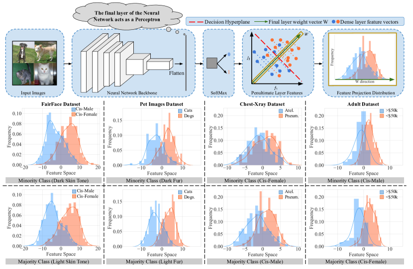
Figure 4: The use of Gaussian mixtures to represent minority and majority distributions is consistent with behaviors in modern neural networks, on real-world datasets. (top row) The last layer of common neural architectures is a linear classifier on features. Histograms of the penultimate layer projections are generated for models with $\beta=0.5$. (middle row) Minority histograms: note the greater difficulty due to less separation of data. (bottom row) Majority histograms: note smaller overlap and easier classification. Figure can be parsed on a per-dataset basis. Within each column, the reader can compare the domain gap and overlap in the two histograms.

In the previous section, we provide existence conditions for the MIME phenomenon for general sample distributions. However, experimental validation of the phenomenon requires quantification in terms of measurable quantities such as overlap. Theorem 2 provides us these resources. Here, we verify that the assumptions in Theorem 2 are validated by experiments on real tasks.

4.1 Verifying Assumptions

Table 1: Experimental measures of overlap and domain gap are consistent with the theory in Section 3. Note that the majority group consistently has lower overlap. Domain gaps are found to be small. DS-1 is FairFace, DS-2 is Pet Images, DS-4 is Chest-Xray14 and DS-5 is Adult. DS-6 is the high domain gap gender classification experiment. DS-3 is excluded here since it deals with a 9 class classification problem.

Dataset (Task)	DS-1 [32] (Gender)	DS-2 [22] (Species)	DS-4 [40] (Diagnosis)	DS-5 [9] (Income)	DS-6 [56, 53] (Gender)
Major. overlap	0.186	0.163	0.294	0.132	0.09
Minor. overlap	0.224	0.198	0.369	0.208	0.19
Domain gap	0.276	0.518	0.494	0.170	1.62

Verifying Gaussianity: Theorem 2 assumes that data $x$ is drawn from a Gaussian Mixture Model. At first glance, this quantification may appear to be unrelated to complex neural networks. However, as illustrated at the top of Figure 4, a ConvNet is essentially a feature extractor that feeds a flattened layer into a simple perceptron or linear classifier. The flattened layer can be orthogonally projected onto the decision boundary to generate, in analogy, an $x$ used for linear classification (Figure 1, fixed-backbone configuration). We use this as a first approximation to the end-to-end configuration used in our experiments.

Plotting empirical histograms of these flattened layers (Figure 4) shows Gaussian-like distribution. This is consistent with the Law of Large Numbers – linear combination of several random variables follows an approximate Gaussian distribution. Hence, Theorem 2 is approximately related in this setting. Details about implementation and comparison to Gaussians are deferred to the supplement.

Verifying minority/majority definitions: The MIME proof linked minority and majority definitions to distributional overlap and domain gap. Given the histogram embeddings from above, it is seen that minority groups on all four vision tasks have greater overlap. There also exists a domain gap between majority and minority but this is small compared to distribution spread (except for the high domain gap experiment). This establishes applicability of small domain gap requirements. Quantification is provided in Table 1. Code is in the supplement.

4.2 MIME Effect Across Six, Real Datasets

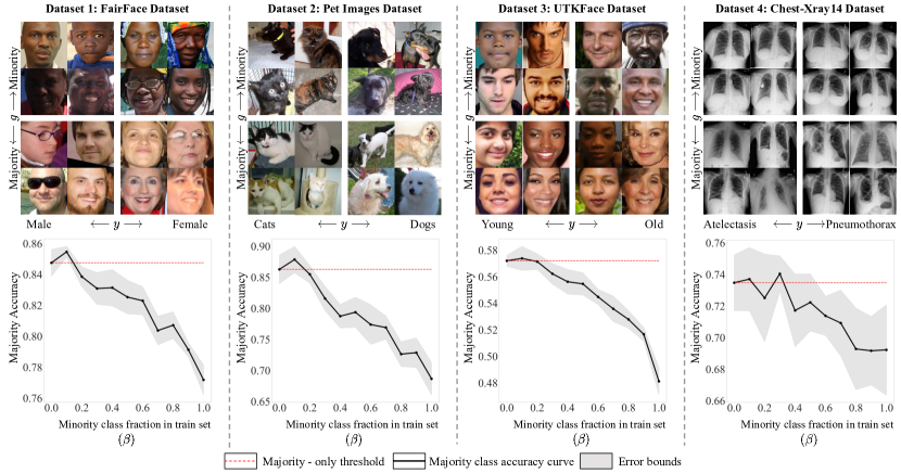
Figure 5: When domain gap is small, the MIME effect holds. On four vision datasets, majority performance is maximized with some inclusion of minorities. All experiments are run for several trials and realizations (described in Section 4.2).

Implementation: Six multi-attribute datasets are used to assess the MIME effect (five are in computer vision). For a particular experiment, we identify a task category to evaluate accuracy over (e.g. gender), and a group category (e.g. race). The best test accuracy on the majority group across all epochs is recorded as our accuracy measure. Each experiment is run for a fixed number of minority training ratios ($\beta$). For each minority training ratio, the total number of training samples remains constant. That is, the minority samples replace the majority samples, instead of being appended to the training set. Each experiment is also run for a finite number of trials. Different trials have different random train and test sets (except for the FairFace dataset [32] where we use the provided test split). Averaging is done across trials. Note that minority samples to be added are randomly chosen – the MIME effect is not specific to particular samples. For the vision datasets, we use a ResNet-34 architecture [25], with the output layer appropriately modified. For the non-visual dataset, a fully connected network is used. Average accuracy and trend error, across trials are used to evaluate performance. Specific implementation details are in the supplement.

MIME effect on gender classification: The FairFace dataset [32] is used to perform gender classification ($y=1$ is male, $y=2$ is female). The majority and minority groups $g=\{\textrm{major},\textrm{minor}\}$ are light and dark skin, respectively. Results are averaged over five trials. Figure 5 describes qualitative accuracy. The accuracy trends indicate that adding 10% of minority samples to the training set leads to approximately a 1.5% gain in majority group (light skin) test accuracy.

MIME effect on animal species identification: We manually annotate light and dark cats and dogs from the Pets dataset [22]. We classify between cats ($y=1$) and dogs ($y=2$). The majority and minority groups are light and dark fur color respectively. Figure 5 shows qualitative results. Over five trials, we see a majority group accuracy gain of about 2%, with a peak at $\beta=$10%.

MIME effect on age classification: We use a second human faces dataset, the UTKFace dataset [56], for the age classification task (9 classes of age-intervals). We pre-process the UTKFace age labels into class bins to match the FairFace dataset format. The majority and minority groups are male and female respectively. The proportion of task class labels is kept the same across group classes. Results are averaged over five trials. Figure 5 shows trends. We observe a smaller average improvement for the 10% minority training ratio. However, since these are average trends, this indicates consistent gain. Results on this dataset also empirically highlight the existence of the MIME effect beyond two class settings.

MIME effect on X-ray diagnosis Classification: We use the NIH Chest-Xray14 dataset [40] to analyze trends on a medical imaging task. We perform binary classification of scans belonging to ‘Atelectasis’ ($y=1$) and ‘Pneumothorax’ ($y=2$) categories. The male and female genders are the majority and minority groups respectively. Results are averaged over seven trials (due to noisier trends). From Figure 5, we observe noisy trends - specifically we see a performance drop for $\beta=0.2$, prior to an overall gain for $\beta=0.3$. The error bounds also have considerably more noise. However, confidence in the peak and the MIME effect, as seen from the average trends and the error bounds, remains high.

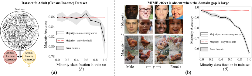
Figure 6: MIME effect is observed in non-vision datasets, and is absent in the case of large domain gap. (a) The Adult Dataset [9] uses Census data to predict an income label. (b) On dataset six, gender classification is rescoped to occur in a high domain gap setting. Majority group is chickens [53] and minority group is humans [56].

MIME effect on income classification: For validation in a non-vision setting, we use the Adult (Census Income) dataset [9]. The data consists of census information with annual income labels (income less than or equal to $50,000 is $y=1$, income greater than $50,000 is $y=2$). The majority and minority groups are female and male genders respectively. Results are averaged over five trials. Figure 6(a) highlights a prominent accuracy gain for $\beta=0.6$.

MIME effect and domain gap: Theorem 2 (Section 3) suggests that large domain gap settings will not show the MIME effect. We set up an experiment to verify this (Figure 6(b)). Gender classification among chickens (majority group) and humans (minority group) has a high domain gap due to minimal common context (validated by the domain gap estimates, Table 1). With increasing $\beta$, the majority accuracy decreases. This (and Figure 4, Table 1 that show low domain gap for other datasets) validates Theorem 2. Note that while this result may not be unexpected, it further validates our proposed theory.

5 Discussion

Secondary validation and analysis: Table 2 supplies additional metrics to analyze MIME. Across datasets, almost all trials show existence, with every dataset showing average MIME performance gain. Some readers may view the error bars in Figures 5 and 6 as large, however they are comparable to other empirical ML works [36, 15]; they may appear larger due to scaling. Reasons for error bars include variations in train-test data and train set size (Table B and C, supplement). Further analysis, including interplay with debiasing methods (e.g. hard-sample mining [18]) and reconciliation with work on equal representation datasets [21, 11, 34, 44, 35, 37, 29, 23, 30] is deferred to the supplement.

Table 2: Additional evaluation metrics provide further evidence of MIME existence across all datasets. The table highlights: (i) number of trials with MIME performance gain (i.e. majority accuracy at some $\beta>0$ is greater than majority accuracy at $\beta=0$), and (ii) the mean MIME performance gain across trials (in % points).

Dataset	DS-1 [32]	DS-2 [22]	DS-3 [56]	DS-4 [40]	DS-5 [9]
#MIME trials/Total trials	4/5	4/5	5/5	6/7	4/5
Avg. MIME perf. gain	0.72%	1.84%	0.70%	1.89%	0.98%

Optimality of inclusion ratios: Our experiments show that there can exist an optimal amount of minority inclusion to benefit the majority group the most. This appears true across all experiments in Figures 5, 6. However, beyond a certain amount, accuracy decreases consistently, with lowest accuracy on majority samples observed when no majorities are used in training. This optimal $\beta$ depends on individual task complexities, among other factors. Since identifying it is outside our scope (Section 1.1, 1.2), our experiments use $10\%$ sampling resolution for $\beta$. Peaks at $\beta=10\%$ for some datasets are due to this lower resolution; optimal peak need not lie there for all datasets (e.g. X-ray [40] & Adult [9]). Future work can identify optimal ratios through finer analysis over $\beta$.

Limitations: The theoretical scope is certifiable within fixed-backbone binary classification, which is narrower than all of machine learning (Figure 1). Should this theory be accepted by the community, follow-up work can generalize theoretical claims. Another limitation is the definition-compatibility of majority and minority groups. Our theory is applicable to task-advantage definitions; some scholars in the community instead define majorities and minorities by proportion. Our theory is applicable to these authors as well, albeit with a slight redefinition of terminology. Additional considerations are included in the supplement.

Conclusion: In conclusion, majority performance benefits from a non-zero fraction of inclusion of minority data given a sufficiently small domain gap.

5.0.1 Acknowledgements

We thank members of the Visual Machines Group for their feedback and support. A.K. was partially supported by an NSF CAREER award IIS-2046737 and Army Young Investigator Award. P.C. was partially supported by a Cisco PhD Fellowship.

References

- [1] Ba, Y., Wang, Z., Karinca, K.D., Bozkurt, O.D., Kadambi, A.: Overcoming difficulty in obtaining dark-skinned subjects for remote-ppg by synthetic augmentation. arXiv preprint arXiv:2106.06007 (2021)
- [2] Balakrishnan, G., Xiong, Y., Xia, W., Perona, P.: Towards causal benchmarking of biasin face analysis algorithms. In: Deep Learning-Based Face Analytics, pp. 327–359. Springer (2021)
- [3] Balcan, M.F., Broder, A., Zhang, T.: Margin based active learning. In: International Conference on Computational Learning Theory. pp. 35–50. Springer (2007)
- [4] Bellamy, R.K., Dey, K., Hind, M., Hoffman, S.C., Houde, S., Kannan, K., Lohia, P., Martino, J., Mehta, S., Mojsilović, A., et al.: Ai fairness 360: An extensible toolkit for detecting and mitigating algorithmic bias. IBM Journal of Research and Development 63(4/5), 4–1 (2019)
- [5] Ben-David, S., Blitzer, J., Crammer, K., Kulesza, A., Pereira, F., Vaughan, J.W.: A theory of learning from different domains. Machine learning 79(1), 151–175 (2010)
- [6] Ben-David, S., Blitzer, J., Crammer, K., Pereira, F., et al.: Analysis of representations for domain adaptation. Advances in Neural Information Processing Systems 19, 137 (2007)
- [7] Beygelzimer, A., Hsu, D.J., Langford, J., Zhang, T.: Agnostic active learning without constraints. Advances in Neural Information Processing Systems 23, 199–207 (2010)
- [8] Bickel, S., Brückner, M., Scheffer, T.: Discriminative learning under covariate shift. Journal of Machine Learning Research 10(9) (2009)
- [9] Blake, C.L., Merz, C.J.: Uci repository of machine learning databases, 1998 (1998)
- [10] Bolukbasi, T., Chang, K.W., Zou, J.Y., Saligrama, V., Kalai, A.T.: Man is to computer programmer as woman is to homemaker? debiasing word embeddings. Advances in Neural Information Processing Systems 29, 4349–4357 (2016)
- [11] Buolamwini, J., Gebru, T.: Gender shades: Intersectional accuracy disparities in commercial gender classification. In: Conference on fairness, accountability and transparency. pp. 77–91. PMLR (2018)
- [12] Chari, P., Kabra, K., Karinca, D., Lahiri, S., Srivastava, D., Kulkarni, K., Chen, T., Cannesson, M., Jalilian, L., Kadambi, A.: Diverse r-ppg: Camera-based heart rate estimation for diverse subject skin-tones and scenes. arXiv preprint arXiv:2010.12769 (2020)
- [13] Choi, J., Elezi, I., Lee, H.J., Farabet, C., Alvarez, J.M.: Active learning for deep object detection via probabilistic modeling. arXiv preprint arXiv:2103.16130 (2021)
- [14] Cui, Y., Jia, M., Lin, T.Y., Song, Y., Belongie, S.: Class-balanced loss based on effective number of samples. In: Proceedings of the IEEE/CVF Conference on Computer Vision and Pattern Recognition. pp. 9268–9277 (2019)
- [15] d’Ascoli, S., Gabrié, M., Sagun, L., Biroli, G.: On the interplay between data structure and loss function in classification problems. Advances in Neural Information Processing Systems 34, 8506–8517 (2021)
- [16] Dasgupta, S.: Two faces of active learning. Theoretical computer science 412(19), 1767–1781 (2011)
- [17] Dasgupta, S., Hsu, D.J., Monteleoni, C.: A general agnostic active learning algorithm. Citeseer (2007)
- [18] Dong, Q., Gong, S., Zhu, X.: Class rectification hard mining for imbalanced deep learning. In: Proceedings of the IEEE/CVF International Conference on Computer Vision. pp. 1851–1860 (2017)
- [19] Elkan, C.: The foundations of cost-sensitive learning. In: International joint conference on artificial intelligence. vol. 17, pp. 973–978. Lawrence Erlbaum Associates Ltd (2001)
- [20] Ertekin, S., Huang, J., Bottou, L., Giles, L.: Learning on the border: active learning in imbalanced data classification. In: Proceedings of the sixteenth ACM conference on Conference on information and knowledge management. pp. 127–136 (2007)
- [21] Gebru, T., Morgenstern, J., Vecchione, B., Vaughan, J.W., Wallach, H., Daumé III, H., Crawford, K.: Datasheets for datasets. arXiv preprint arXiv:1803.09010 (2018)
- [22] Golle, P.: Machine learning attacks against the asirra captcha. In: Proceedings of the 15th ACM conference on Computer and communications security. pp. 535–542 (2008)
- [23] Gong, Z., Zhong, P., Hu, W.: Diversity in machine learning. IEEE Access 7, 64323–64350 (2019)
- [24] Gwilliam, M., Hegde, S., Tinubu, L., Hanson, A.: Rethinking common assumptions to mitigate racial bias in face recognition datasets. In: Proceedings of the IEEE/CVF International Conference on Computer Vision. pp. 4123–4132 (2021)
- [25] He, K., Zhang, X., Ren, S., Sun, J.: Deep residual learning for image recognition. In: Proceedings of the IEEE/CVF Conference on Computer Vision and Pattern Recognition. pp. 770–778 (2016)
- [26] Hendricks, L.A., Burns, K., Saenko, K., Darrell, T., Rohrbach, A.: Women also snowboard: Overcoming bias in captioning models. In: Proceedings of the European Conference on Computer Vision (ECCV). pp. 771–787 (2018)
- [27] Huang, J., Guan, D., Xiao, A., Lu, S.: Fsdr: Frequency space domain randomization for domain generalization. In: Proceedings of the IEEE/CVF Conference on Computer Vision and Pattern Recognition. pp. 6891–6902 (2021)
- [28] Huang, S.J., Jin, R., Zhou, Z.H.: Active learning by querying informative and representative examples. Advances in Neural Information Processing Systems 23, 892–900 (2010)
- [29] Jo, E.S., Gebru, T.: Lessons from archives: Strategies for collecting sociocultural data in machine learning. In: Proceedings of the 2020 Conference on Fairness, Accountability, and Transparency. pp. 306–316 (2020)
- [30] Kadambi, A.: Achieving fairness in medical devices. Science 372(6537), 30–31 (2021)
- [31] Kang, B., Xie, S., Rohrbach, M., Yan, Z., Gordo, A., Feng, J., Kalantidis, Y.: Decoupling representation and classifier for long-tailed recognition. arXiv preprint arXiv:1910.09217 (2019)
- [32] Karkkainen, K., Joo, J.: Fairface: Face attribute dataset for balanced race, gender, and age for bias measurement and mitigation. In: Proceedings of the IEEE/CVF Winter Conference on Applications of Computer Vision. pp. 1548–1558 (2021)
- [33] Kremer, J., Steenstrup Pedersen, K., Igel, C.: Active learning with support vector machines. Wiley Interdisciplinary Reviews: Data Mining and Knowledge Discovery 4(4), 313–326 (2014)
- [34] Larrazabal, A.J., Nieto, N., Peterson, V., Milone, D.H., Ferrante, E.: Gender imbalance in medical imaging datasets produces biased classifiers for computer-aided diagnosis. Proceedings of the National Academy of Sciences 117(23), 12592–12594 (2020)
- [35] Li, Y., Vasconcelos, N.: Repair: Removing representation bias by dataset resampling. In: Proceedings of the IEEE/CVF Conference on Computer Vision and Pattern Recognition. pp. 9572–9581 (2019)
- [36] Liu, T., Vietri, G., Wu, S.Z.: Iterative methods for private synthetic data: Unifying framework and new methods. Advances in Neural Information Processing Systems 34, 690–702 (2021)
- [37] Mehrabi, N., Morstatter, F., Saxena, N., Lerman, K., Galstyan, A.: A survey on bias and fairness in machine learning. ACM Computing Surveys (CSUR) 54(6), 1–35 (2021)
- [38] Mohri, M., Rostamizadeh, A.: Perceptron mistake bounds. arXiv preprint arXiv:1305.0208 (2013)
- [39] Nowara, E.M., McDuff, D., Veeraraghavan, A.: A meta-analysis of the impact of skin tone and gender on non-contact photoplethysmography measurements. In: Proceedings of the IEEE/CVF Conference on Computer Vision and Pattern Recognition Workshops. pp. 284–285 (2020)
- [40] Rajpurkar, P., Irvin, J., Zhu, K., Yang, B., Mehta, H., Duan, T., Ding, D., Bagul, A., Langlotz, C., Shpanskaya, K., et al.: Chexnet: Radiologist-level pneumonia detection on chest x-rays with deep learning. arXiv preprint arXiv:1711.05225 (2017)
- [41] Ramaswamy, V.V., Kim, S.S., Russakovsky, O.: Fair attribute classification through latent space de-biasing. In: Proceedings of the IEEE/CVF Conference on Computer Vision and Pattern Recognition. pp. 9301–9310 (2021)
- [42] Redko, I., Morvant, E., Habrard, A., Sebban, M., Bennani, Y.: A survey on domain adaptation theory: learning bounds and theoretical guarantees. arXiv preprint arXiv:2004.11829 (2020)
- [43] Ren, M., Zeng, W., Yang, B., Urtasun, R.: Learning to reweight examples for robust deep learning. In: International Conference on Machine Learning. pp. 4334–4343. PMLR (2018)
- [44] Ryu, H.J., Adam, H., Mitchell, M.: Inclusivefacenet: Improving face attribute detection with race and gender diversity. arXiv preprint arXiv:1712.00193 (2017)
- [45] Settles, B.: Active learning literature survey (2009)
- [46] Tartaglione, E., Barbano, C.A., Grangetto, M.: End: Entangling and disentangling deep representations for bias correction. In: Proceedings of the IEEE/CVF Conference on Computer Vision and Pattern Recognition. pp. 13508–13517 (2021)
- [47] Tremblay, J., Prakash, A., Acuna, D., Brophy, M., Jampani, V., Anil, C., To, T., Cameracci, E., Boochoon, S., Birchfield, S.: Training deep networks with synthetic data: Bridging the reality gap by domain randomization. In: Proceedings of the IEEE/CVF Conference on Computer Vision and Pattern Recognition Workshops. pp. 969–977 (2018)
- [48] Vilesov, A., Chari, P., Armouti, A., Harish, A.B., Kulkarni, K., Deoghare, A., Jalilian, L., Kadambi, A.: Blending camera and 77 ghz radar sensing for equitable, robust plethysmography. In: ACM Trans. Graph. (SIGGRAPH) (2022)
- [49] Wang, T., Zhao, J., Yatskar, M., Chang, K.W., Ordonez, V.: Balanced datasets are not enough: Estimating and mitigating gender bias in deep image representations. In: Proceedings of the IEEE/CVF International Conference on Computer Vision. pp. 5310–5319 (2019)
- [50] Wang, Z., Qinami, K., Karakozis, I.C., Genova, K., Nair, P., Hata, K., Russakovsky, O.: Towards fairness in visual recognition: Effective strategies for bias mitigation. In: Proceedings of the IEEE/CVF Conference on Computer Vision and Pattern Recognition. pp. 8919–8928 (2020)
- [51] Wang, Z., Ba, Y., Chari, P., Bozkurt, O.D., Brown, G., Patwa, P., Vaddi, N., Jalilian, L., Kadambi, A.: Synthetic generation of face videos with plethysmograph physiology. In: Proceedings of the IEEE/CVF Conference on Computer Vision and Pattern Recognition (CVPR). pp. 20587–20596 (2022)
- [52] Xu, H., Liu, X., Li, Y., Jain, A., Tang, J.: To be robust or to be fair: Towards fairness in adversarial training. In: International Conference on Machine Learning. pp. 11492–11501. PMLR (2021)
- [53] Yao, Y., Yu, H., Mu, J., Li, J., Pu, H.: Estimation of the gender ratio of chickens based on computer vision: Dataset and exploration. Entropy 22(7), 719 (2020)
- [54] Yue, X., Zhang, Y., Zhao, S., Sangiovanni-Vincentelli, A., Keutzer, K., Gong, B.: Domain randomization and pyramid consistency: Simulation-to-real generalization without accessing target domain data. In: Proceedings of the IEEE/CVF International Conference on Computer Vision. pp. 2100–2110 (2019)
- [55] Zhang, B.H., Lemoine, B., Mitchell, M.: Mitigating unwanted biases with adversarial learning. In: Proceedings of the 2018 AAAI/ACM Conference on AI, Ethics, and Society. pp. 335–340 (2018)
- [56] Zhang, Z., Song, Y., Qi, H.: Age progression/regression by conditional adversarial autoencoder. In: Proceedings of the IEEE/CVF Conference on Computer Vision and Pattern Recognition. pp. 5810–5818 (2017)