Self-supervised Representation Learning on Electronic Health Records with Graph Kernel Infomax

Abstract

Learning Electronic Health Records (EHRs) representation is a preeminent yet under-discovered research topic. It benefits various clinical decision support applications, e.g., medication outcome prediction or patient similarity search. Current approaches focus on task-specific label supervision on vectorized sequential EHR, which is not applicable to large-scale unsupervised scenarios. Recently, contrastive learning shows great success on self-supervised representation learning problems. However, complex temporality often degrades the performance. We propose Graph Kernel Infomax, a self-supervised graph kernel learning approach on the graphical representation of EHR, to overcome the previous problems. Unlike the state-of-the-art, we do not change the graph structure to construct augmented views. Instead, we use Kernel Subspace Augmentation to embed nodes into two geometrically different manifold views. The entire framework is trained by contrasting nodes and graph representations on those two manifold views through the commonly used contrastive objectives. Empirically, using publicly available benchmark EHR datasets, our approach yields performance on clinical downstream tasks that exceeds the state-of-the-art. Theoretically, the variation on distance metrics naturally creates different views as data augmentation without changing graph structures.

Introduction

Representation learning of patient Electronic Health Records (EHRs) is the foundation for data-driven personalized healthcare and clinical decision support (Yadav et al. 2017). Many approaches, in particular deep learning models, were proposed to learn EHR representation (Choi et al. 2016; Ma et al. 2017; Xu et al. 2018b; Choi et al. 2020; Yao et al. 2020). However, all of them rely on task-specific label supervision. Annotation on large-scale EHR is challenging, thus, not ideal for an unknown clinical problem with unlabeled medical records, e.g., patient similarity search (Parimbelli et al. 2018). Autoencoders  (Miotto et al. 2016; Lyu et al. 2018) provide the option for unsupervised learning. But, sparse medical coding and lengthy temporal sequences often lead to poor reconstruction loss optimization. Though the BERT-based language model (Li et al. 2020) shows the remarkable clinical document pre-training, it still requires downstream clinical task fine-tuning to obtain promising performance. Yet, a universal representation is still lacking.

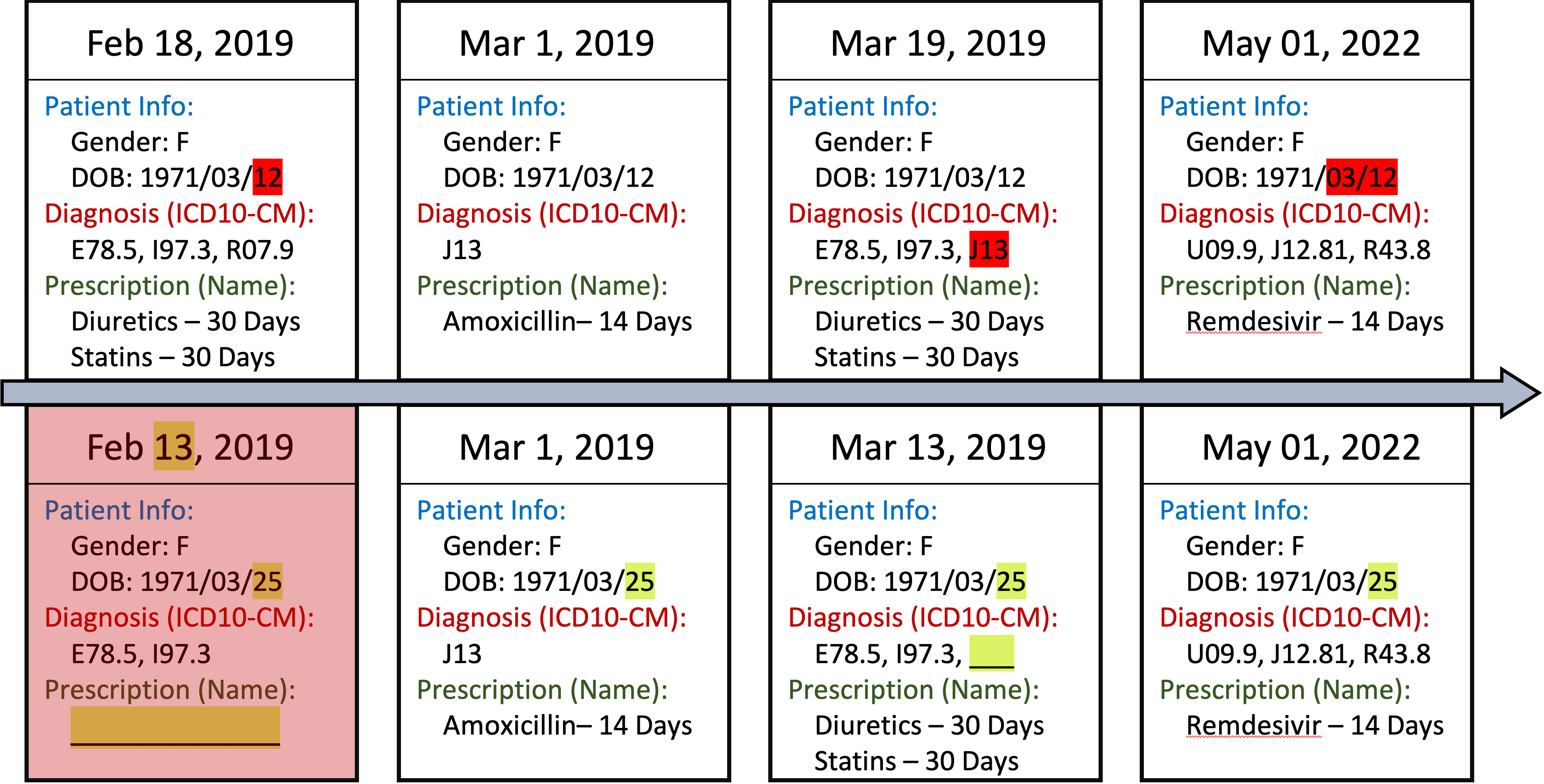
On the other hand, contrastive learning has shown state-of-the-art performance in a fully unsupervised setting, e.g., without fine-tuning, in computer vision (Chen et al. 2020) and graph representation learning (Velickovic et al. 2019). It has been applied to EHR representation learning and achieves superior effort in several clinical downstream tasks (Yèche et al. 2021). However, data augmentation on the long-time span of high variance and temporality of EHR often causes view ambiguity: the similarity increases on negative samples but decreases on the positive one. As in Figure 1, two highly similar patients but reside in different target cohort groups become even more similar after random history crop and gaussian noise (Yèche et al. 2021). Thus, designing a proper semantic-preserving data augmentation without modification to the original data with such EHR complexity is necessary to overcome these challenges.

Figure 1: View ambiguity. There are seven differences, highlighted in light green, between two target cohorts of highly similar patients A (above) and B (below). Data augmentation, highlighted in red, e.g., history crop (removing the first clinical visit of B) and gaussian noise (masking out DOB day and diagnosis code in A), however, decreases their mismatched fields and possibly increases their similarity.

Addressing these challenges, we design a theoretically and empirically sound self-supervised, contrastive graph kernel learning approach, namely, Graph Kernel Infomax (GKI). Compressing feature temporality and heterogeneity of EHR via graph, we learn graph kernel feature maps with a graphical representation of EHR to model universal patient representation. Instead of modifying graph topologies for augmentation, we propose Kernel Subspace Augmentation to embed nodes into two manifolds yielded by different kernels with different underlying metrics. The embedding of node and graph on two manifolds act as augmented views for commonly used contrastive loss. We geometrically analyze data augmentation under a local-neighborhood perspective and reveal that adjusting distance metrics in the underlying manifold can achieve the same effect as the augmentation on graph structure. By maximizing Mutual Information (MI) between node and graph in these two manifolds, our patient representation can directly apply to linear models on clinical tasks without fine-tuning and label supervision. To our best knowledge, this is the first effort for self-supervised representation on EHR without any task-specific supervision. Furthermore, our method achieves superior or at least competitive performance on other graph benchmarks, revealing its non-ad hoc generalizability and robustness to handle unknown problems. Our contributions are as follows:

• We propose Graph Kernel Infomax for self-supervised representation learning on EHR without the need to modify graph structures for data augmentation.

• We develop and provide theoretical analysis on Kernel Subspace Augmentation by embedding nodes and graph to geometrically different manifolds via a kernel method to construct augmented views.

• We experiment with a large-scale, publicly available EHR dataset to demonstrate our effectiveness on clinical downstream tasks.

• We validate our non-ad hoc generalizability and robustness with widely used graph benchmark datasets.

Related Work

EHR representation learning

Many efforts focus on EHR representation learning (Choi et al. 2016; Ma et al. 2017; Yadav et al. 2017). Besides the autoencoder-based model (Miotto et al. 2016), there is less work on unsupervised method. One reason is the non-trivial design of training signals without label supervision for complex EHR (Shickel et al. 2017). The large-scale pre-trained language model trained on large-scale EHR shows promising results on various clinical downstream tasks (Li et al. 2020). The recently proposed contrastive learning method (Chen et al. 2020) shines a new light on learning effective representation without task-specific fine-tuning. It further demonstrates the utility of medical representation learning (Yèche et al. 2021). Nonetheless, current work only applies to time-series of Intensive Care Units (ICU) and EEG. Yet, the unsupervised EHR representation learning is not fully solved. Recently, (Sun et al. 2020; Qiu et al. 2020; Hassani and Khasahmadi 2020; You et al. 2020) introduce several augmentation strategies, namely corrupting graph topology, to construct different views for contrastive learning and achieve state-of-the-art. However, such method may construct less informative views due to data complexity, where our evaluation confirms the difficulty of clinical application.

Manifold Learning with Kernel

A manifold (e.g., Riemannian manifold) locally approximates Euclidean space for non-linear data that resides on spheres or hyperbolic spaces. It is well-known that Symmetric Positive Definite (SPD) matrices form a Riemannian manifold (Jayasumana et al. 2013; Dong et al. 2017). Despite the difficulty of operation on SPD matrices, several methods were proposed to approximate SPD manifold (Dong et al. 2017), for instance, the kernel method, which embeds a Riemannian manifold into a high dimensional Reproducing Kernel Hilbert Space (RKHS) (Jayasumana et al. 2013) via positive definite kernel, where an inner product is naturally applied. In  (Zhang and Davison 2021), a spherical manifold is approximated by Gaussian Kernel for unsupervised domain adaptation. The distance metric, defining a kernel function, is also investigated in (Feragen, Lauze, and Hauberg 2015), which leads to the generalization of certain shape of a manifold, e.g., geodesic Laplacian kernel for a spherical manifold.

Figure 2: A sample patient EHRs.

Figure 3: An example of a patient graph reflecting the first three medical events in Figure 3

Figure 4: Graph Kernel Infomax. We first obtain node embeddings from the GNN $f_{\theta}$ followed by K-means clustering $f_{\mathcal{C}}$. The resulting cluster centroids $\mathcal{C}$ are used as landmark points for the nyström kernel approximation to construct kernel feature maps ${\phi}_{E}$ and ${\phi}_{S}$ for Euclidean and spherical distance kernels. The two kernel embeddings for nodes and graph are contrasted to compute final losses.

Methodology

In this section, we present Graph Kernel Infomax (GKI), a self-supervised contrastive learning framework for learning kernel feature maps for the graphical representation of EHR. Figure 4 illustrates the architecture of GKI.

Problem Definition

Let $G_{s}=\{G_{1},G_{2},\ldots\}$ be a set of graphs (EHR graphs) and $G_{i}\in G_{s}$ denotes $i$-th patient EHR graph. For each $G_{i}=(X_{i},A_{i})$ containing $n$ nodes, we denote the node feature matrix and adjacency matrix as $X_{i}\in\mathbb{R}^{n\times D}$ and $A_{i}\in\mathbb{R}^{n\times n}$, where each node is a $D$-dimensional feature vector in $X_{i}$, and an edge connection between two nodes is either binary or weighted in $A_{i}$. Our goal is to learn graph-level kernel feature maps $\Phi_{E},\Phi_{S}$ derived from Euclidean distance and spherical distance kernels without label supervision via contrastive learning. The resulting graph-level kernel embeddings $\Phi_{E}(G_{i})$ and $\Phi_{S}(G_{i})$, acting as patient representation under Euclidean and spherical distance kernels, can be directly supplied to downstream task models, e.g., linear SVM. It also benefits from the kernel method and multiple kernel properties from two kernels providing efficient non-linear learning for linear classifiers and similarity search on large-scale EHR. We summarize Graph Kernel Infomax in Figure 4.

EHR Graphical Representation

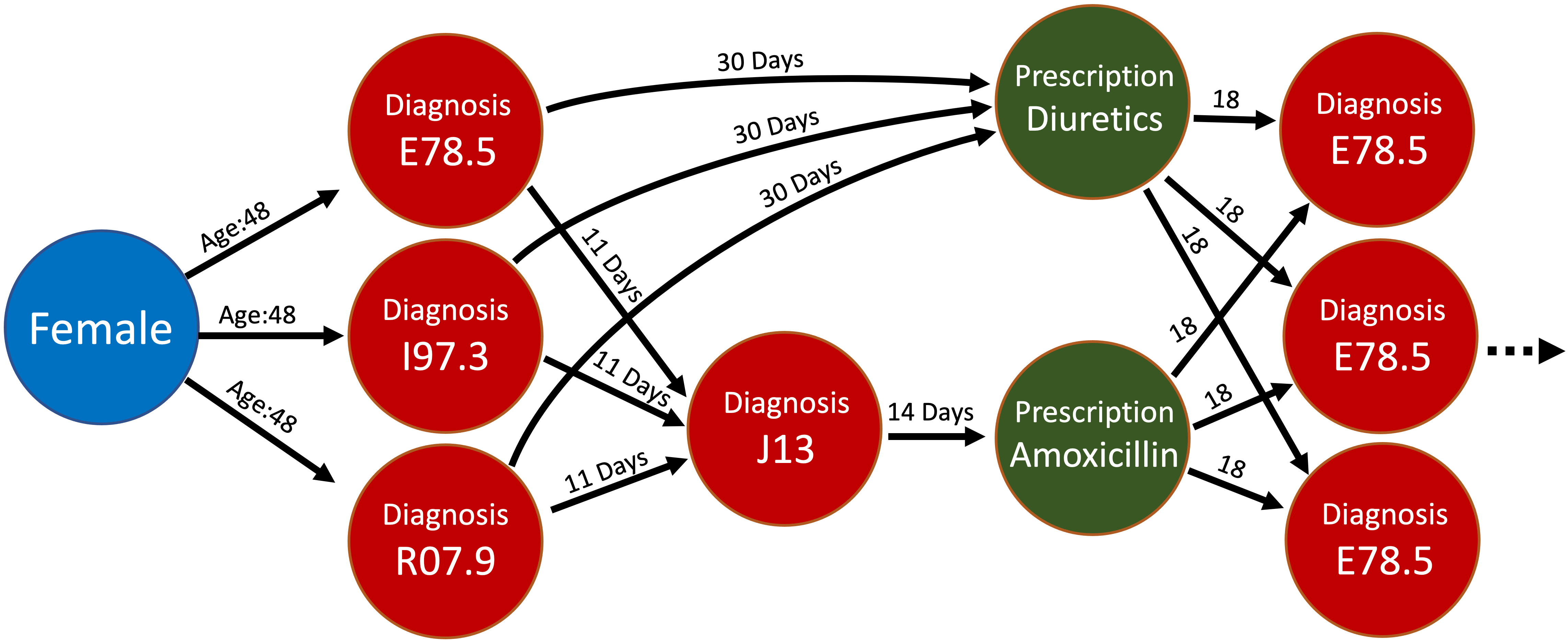
We formulate a patient’s EHR, Figure 3, as a directed graph following the definition in (Yao et al. 2020), except we do not impose directed-acyclic properties. Every medical event, including a disease diagnosis, a drug prescription, and other medical codes, is represented as a node with one-hot encoding. The edge between two nodes represents an ordered direct connection with the time difference as an edge weight (e.g., days or prescription period). Note, we assume the duration for an event is the prescription period, and any medical event in between will create another branch for connection. The demographic information of the patient, e.g., gender, connects to the first medical event with age as an edge weight. Figure 3 shows an example of a graphical representation of an EHR. As we can see, we retain overlaps between medical events instead of connecting sequentially to preserve their original temporal structure. The construction steps are described in the supplementary material.

Graph Kernel Feature Map

We construct graph-level kernel feature map $\Phi$ given with a RKHS kernel $k$ by the following components: (1) graph encoder, (2) K-means clustering, and (3) Node-level feature map via Nyström kernel approximation (Drineas, Mahoney, and Cristianini 2005).

Graph Representation Learning

Given a patient graph $G_{i}=(X_{i},A_{i})$, we derive its $l$-th layer $d$-dimensional node representation via graph nerual networks (GNNs) as:

$$h^{(l)}_{i}=f_{\theta}(X_{i},A_{i})\in\mathbb{R}^{n\times d}$$ (1)

where $f_{\theta}$ denotes a GNN layer, and we allow other choices of GNN architecture.

K-Means Clustering

Nyström method avoids computing the full-rank kernel matrix by landmark selection, which is critical to approximation quality. We adopt K-means clustering, which has proven to generate a good kernel approximation (Zhang and Kwok 2010), and select cluster centroids as landmarks. To enable end-to-end mini-batch training, we develop a $l$-th layer K-means clustering $f_{\mathcal{C}^{(l)}}$ to partitions $h^{(l)}_{i}$ into $K$ clusters:

$$H^{(l)}_{i}=f_{\mathcal{C}^{(l)}}(h^{(l)}_{i})=\sigma(h^{(l)}_{i}{C^{(l)}}^{T})$$ (2)

where $C^{(l)}\in\mathbb{R}^{K\times d}$ denotes $l$-th layer $K$ randomly initialized cluster centroids, $\sigma(\cdot)$ is the sparse-softmax activation function (Martins and Astudillo 2016) and $H^{(l)}_{i}\in\mathbb{R}^{n\times K}$ is the clustering assignment for $h^{(l)}_{i}$. The associated clustering loss for $h^{(l)}_{i}$ is defined as:

$${\mathcal{L}_{i}}^{\text{rec}^{(l)}}={\lVert h_{i}^{(l)}-H^{(l)}_{i}C^{(l)}_{i}\rVert}_{F}$$ (3)

where ${\lVert\cdot\rVert}_{F}$ denotes frobenius norm. The final clustering loss is computed from all layers as ${\mathcal{L}_{i}}^{\text{rec}}=\sum^{L}_{l=1}{\mathcal{L}_{i}}^{\text{rec}^{(l)}}$.

Graph-level Kernel Feature Map

To construct graph-level kernel feature map, we first define $l$-th layer node-level kernel feature map for $h^{(l)}_{i}$ given $\mathcal{C}^{(l)}=\{c^{(l)}_{1},\cdots,c^{(l)}_{K}\}$ selected as landmark points as:

$$\phi(h^{(l)}_{i})=[k(h^{(l)}_{i},c^{(l)}_{1}),\ldots,k(h^{(l)}_{i},c^{(l)}_{K})]\hat{\kappa}^{\dagger}\in\mathbb{R}^{n\times K}$$ (4)

where $\hat{\kappa}_{ij}=k(c_{i},c_{j})$ is the pseudo-inverses of $\mathcal{K}\in\mathbb{R}^{K\times K}$ where $\mathcal{K}_{ij}=k(c_{i},c_{j})$. One interesting observation is that, by setting the pseudo-inverse $\hat{\kappa}^{\dagger}$ to $\mathbin{I}$, we found a dramatic performance improvement in our evaluation. We believe such an effect leads to orthogonal constraints on landmark points that act as orthogonal regularizations to avoid trivial solutions in K-means clustering. We leave it here for future research work. We then derive the graph-level kernel feature map for the entire graph. In order to preserve high-order information of graph, we concatenate the summation on the node-level kernel feature map in each layer:

$$\Phi(G_{i})=\bigparallel_{l=1}^{L}\left[\sum^{n}_{j=1}{\phi(h^{(l)}_{i})}_{j}\right]\in\mathbb{R}^{KL}$$ (5)

Kernel Subspace Augmentation

The graph kernel feature map $\Phi$ is parameterized by GNN layers and K-Means clustering. To learn optimal model parameters without label supervision, we formulate it as graph contrastive learning. To design an augmentation scheme without modification to the original graph, we seek another interpretation on contrastive learning:

Observation 1

(Ko et al. 2022) Given a positive pair $z_{i},z_{j}$, minimizing the contrastive loss for $z_{i},z_{j}$ is equivalent to maximizing the probability that $z_{j}$, the positive pair of $z_{i}$, is the 1-nearest neighbor (1-NN) of $z_{i}$. Therefore, contrastive Learning can be considered as optimizing 1-Nearest Neighbor problem.

Data Augmentation via Distance Metrics

Observation 1 provides an intuitive explanation of explicit augmentation, which adds negative samples to create perturbation in the local neighborhood for each sample. Such perturbation alters 1-NN by adding noise in the local proximity of positive pairs in their projection space, providing signals for contrastive loss to minimize. Considering a smooth compact $d$-dimensional Riemannian manifold $\mathcal{M}$ and its true geodesic distance $d_{\mathcal{M}}$ (Li and Dunson 2019), We define two distance metrics on $\mathcal{M}$, namely Euclidean and spherical distance, to approximate the true underlying geodesic distance $d_{M}$:

Definition 1

Euclidean Distance. The Euclidean distance $d_{E}$ between two arbitrary points $x_{i}$ and $x_{j}$ on $\mathcal{M}$ is defined as

$$d_{E}(x_{i},x_{j})={\lVert x_{i}-x_{j}\rVert}_{2}.$$ (6)

Definition 2

Spherical Distance. Let $S$ be a $d$-dimensional $r$-radius sphere centered at $c$ on $\mathcal{M}$ and $\pi$ be the orthogonal projection from the $\mathcal{M}$ to $S$, the spherical distance between two arbitrary points $x_{i}$ and $x_{j}$ on $\mathcal{M}$ is defined as

$$d_{S}(x_{i},x_{j})=r\text{arccos}(\frac{\pi(x_{i})-c}{r}\cdot\frac{\pi(x_{j})-c}{r}).$$ (7)

Figure 5: Neighborhood difference. The green, red, and blue three points are measured with geodesic distance (purple) and Euclidean distance (orange). After projecting to the shared space via $f$ from their source manifold, we can see the nearest neighbor for the red point is changed.

Theorem 1

Distance Variation Bound. Given two arbitrary sufficiently close neighbors $x_{i}$ and $x_{j}$ on $\mathcal{M}$, the following inequality holds when the true underlying geodesic distance between $x_{i}$ and $x_{j}$ is $m$ such that $d_{\mathcal{M}}(x_{i},x_{j})=m$,

$$-O(m^{4})\leq d_{S}(x_{i},x_{j})-d_{E}(x_{i},x_{j})\leq O(m^{3}).$$ (8)

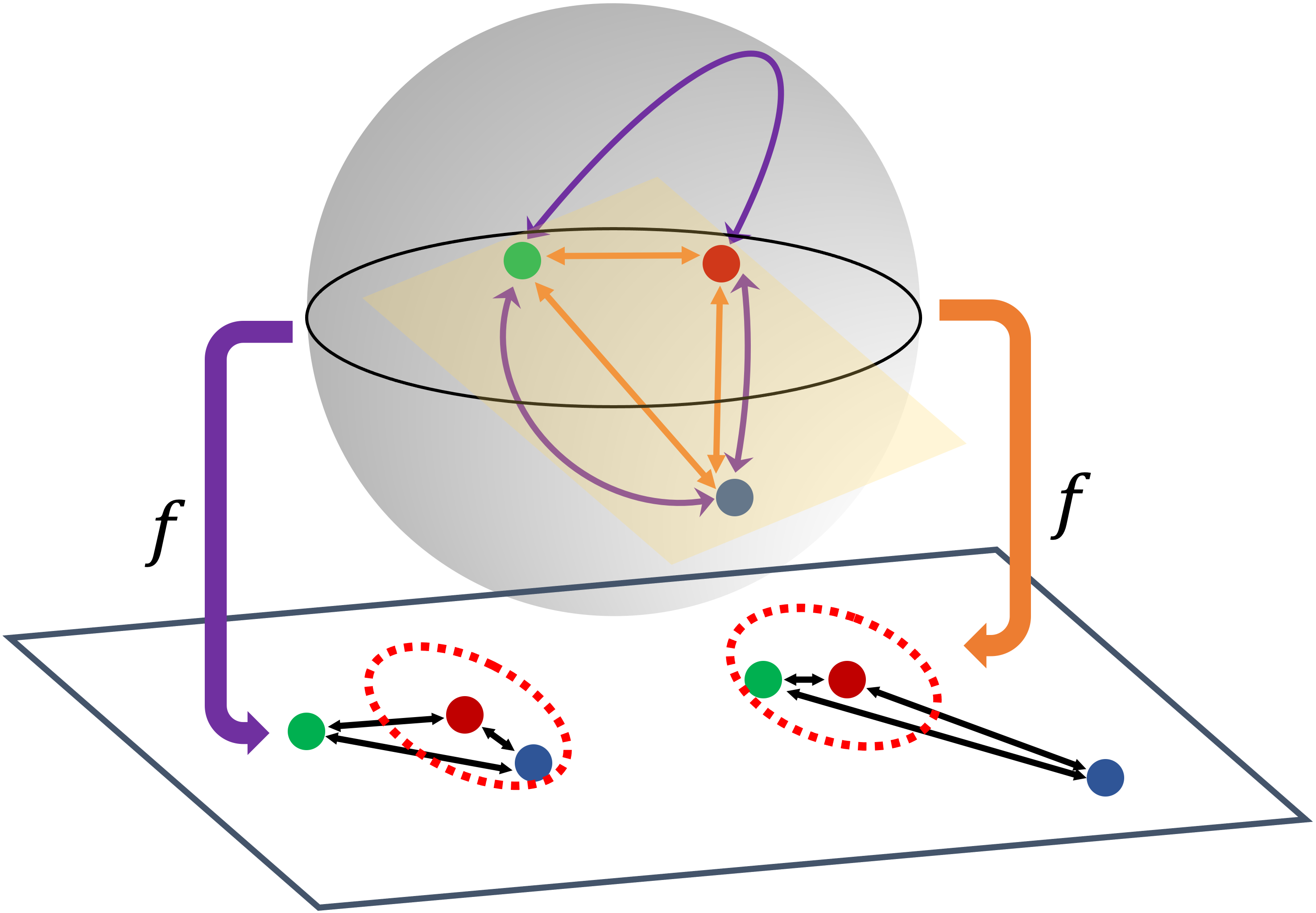
The proof for Theorem 1 can be found in the supplementary material, where we mainly extend the results from (Li and Dunson 2019). By Theorem 1, we show that perturbation can be created by varying distance metrics to affect the distance calculation between two arbitrary points in their local-neighborhood. Such a perturbation alters 1-NN for each sample on two different manifolds. Namely, the positive pair for each sample now becomes the same data point but the embeddings on two manifolds, respectively. As illustrated in Figure 5, when projecting them to the space where contrastive loss is applied, the 1-NN for each sample will not be identical due to the perturbation on their local-neighborhood distance calculation. This inconsistency acts as a contrastive signal to optimize the model. The error between two distance measures in local-neighborhood is also bounded as shown in Theorem 1 resulting in stable training since the model will not overfit on a certain distance metric. Empirically, our model can converge to a lower minimum as described in Figure 7.

Manifolds as Augmented Views

Referring to related work, a positive definite kernel embeds a Riemannian manifold into RKHS (Jayasumana et al. 2013). Moreover, Nyström kernel approximation aims to find a subspace $\mathcal{H}^{\prime}$, which spanned by landmark points $\mathcal{C}$, under kernel induced RKHS (Vedaldi and Zisserman 2012). Hence, we can interpret Nyström kernel feature maps as an efficient mapping that embeds input to its respective Riemannian manifolds. Applying Theorem 1, we are now finding two Riemannian manifolds with different underlying metrics that act as augmented views. As a result, we define two positive definite kernels with Euclidean and spherical distance:

Definition 3

Euclidean and Spherical Kernels. Given two samples $x$ and $y$, the Euclidean kernel $k_{E}$ and spherical kernel $k_{S}$ are defined as

$$\begin{split}k_{E}(x,y)&=\exp(-d_{E}(x,y)),\\ k_{S}(x,y)&=\exp(-d_{S}(x,y)).\end{split}$$ (9)

It is already known that $k_{E}$, the Euclidean kernel, is a positive definite kernel. For $k_{S}$, we can refer (Feragen, Lauze, and Hauberg 2015) such that the Laplacian kernel, as the formulation in Definition 3, is positive definite when geodesic distance is used. Since we have two RKHS kernels, we can define their node and graph kernel feature maps under Euclidean kernel as $\Phi_{E},\phi_{E}$ and spherical kernel as $\Phi_{S},\phi_{S}$, respectively. Given a patient graph $G_{i}=(X_{i},A_{i})$ and last layer node representation $h_{i}$, we now define the augmented views as:

$$h^{E}_{i} =\phi_{E}(h_{i})$$ (10)

$$h^{S}_{i} =\phi_{S}(h_{i})$$ (11)

$$g^{E}_{i} =\Phi_{E}(G_{i})$$ (12)

$$g^{E}_{i} =\Phi_{S}(G_{i})$$ (13)

where $h^{E}_{i},h^{S}_{i}$ denote node Euclidean and spherical views and $g^{E}_{i},g^{S}_{i}$ denotes graph Euclidean and spherical view, respectively.

Training Graph Kernel Infomax

We now formally present Graph Kernel Infomax (GKI) and its training procedure. GKI maximizes MI by contrasting node Euclidean view and graph Spherical view and vice versa. As we discovered, some patients contain a long history in their EHR resulting in larger graphs, while others are small. Such variation on graph size with EHR augmentation ambiguity easily makes the model overfit on certain local structures or global representations. To overcome such complex EHR problems, we contrast both node-graph and graph-graph representations.

We randomly sample size $N$ mini-batch $\mathcal{B}$ from $G_{s}$ for training. We train Graph Kernel Infomax via normalized temperature-scaled cross entropy loss (NT-Xent) (Chen et al. 2020). For positive pair $p,q$, we define the contrastive loss:

$$\ell_{cl}(p,q)=-log\frac{e^{\mathrm{sim}(p,q)/\tau}}{\sum_{q\prime\in\mathcal{B}}\mathbbm{1}_{[p\neq q\prime]}e^{\mathrm{sim}(p,q\prime)/\tau}}$$ (14)

where $\text{sim}(\cdot)$ denotes cosine similarity and $\mathbbm{1}_{[p\neq q\prime]}\in\{0,1\}$ defines an indicator function. Under correlated views for $G_{i}\in\mathcal{B}$, its node Euclidean and spherical views $h^{E}_{i}$, $h^{S}_{i}$, and graph Euclidean and spherical views $g^{E}_{i}$, $g^{S}_{i}$ are projected to a shared embedding space $\mathbb{R}^{d_{p}}$ by node projection head $f_{\alpha}$ and graph projection head $f_{\beta}$, producing projected nodes $\hat{h}^{E}_{i}\in\mathbb{R}^{n\times d_{p}}$, $\hat{h}^{S}_{i}\in\mathbb{R}^{n\times d_{p}}$ and projected graphs $\hat{g}^{E}_{i}\in\mathbb{R}^{d_{p}}$, $\hat{g}^{S}_{i}\in\mathbb{R}^{d_{p}}$. The projection heads are discarded after training. We define node-graph contrastive loss ${\mathcal{L}_{i}}^{\text{N-G}}$ and graph-graph contrastive loss ${\mathcal{L}_{i}}^{\text{G-G}}$ for $G_{i}\in\mathcal{B}$ as follows:

$${\mathcal{L}_{i}}^{\text{N-G}}=\sum_{\hat{z}_{E}\in\hat{h}^{E}_{i}}\sum_{\hat{z}_{S}\in\hat{h}^{S}_{i}}\ell_{cl}(\hat{z}_{E},\hat{g}^{S}_{i})+\ell_{cl}(\hat{z}_{S},\hat{g}^{E}_{i})$$ (15)

$${\mathcal{L}_{i}}^{\text{G-G}}=\ell_{cl}(\hat{g}^{E}_{i},\hat{g}^{S}_{i})+\ell_{cl}(\hat{g}^{S}_{i},\hat{g}^{E}_{i})$$ (16)

The final loss $\mathcal{L}$ is the summation of all losses defined so far for all graphs in $B$:

$$\mathcal{L}=\sum^{N}_{i=1}{\mathcal{L}_{i}}^{\text{N-G}}+{\mathcal{L}_{i}}^{\text{G-G}}+{\mathcal{L}_{i}}^{\text{rec}}$$ (17)

We optimize Graph Kernel Infomax by using mini-batch Stochastic Gradient Descent to minimize mini-batch loss $\mathcal{L}$. Note, the clustering loss is optimized jointly with contrastive loss to encourage both graph encoder and clustering to learn a clustering-friendly representation as in (Yang et al. 2017).

It should be noticed that our method is different from the parallel work (Yang et al. 2022), although they perform similar graph contrastive learning between Euclidean and hyperbolic space embeddings. First, we are completely unsupervised, while they require label supervision. Second, we create perturbation from distance metrics with theoretical justification, however, it is unclear whether hyperbolic space achieves similar outcomes. Third, we approximate manifolds via kernel feature maps, which directly apply to downstream linear models instead of neural space transformation with end-to-end training. In this case, we decouple pretraining and downstream tasks to achieve more generalizability.

Experiments

Table 1: Performance comparison on clinical evaluation tasks under AUROC and F1-Macro in percentages. All scores are averaged over 5 times repeated 10-folds cross validation with their standard deviation reported. Scores with boldface denote the best result. In each baseline group, the underline scores stand for the best in the group. GKI achieves state-of-the-art results.

	Diabetes		Hypertension		Hyperlipidemia		Patient Similarity Search
Model	AUROC	F1-Macro	AUROC	F1-Macro	AUROC	F1-Macro	Precision@1	Precision@10
Retain	49.6 ± 0.2	49.0 ± 0.1	50.0 ± 0.3	49.0 ± 0.1	50.0 ± 0.2	49.2 ± 0.1	-	-
Dipole	50.0 ± 0.2	49.0 ± 0.1	50.0 ± 0.2	50.0 ± 0.1	49.9 ± 0.2	49.4 ± 0.1	-	-
GCT	49.6 ± 0.3	47.9 ± 0.0	50.0 ± 0.2	48.2 ± 0.1	50.4 ± 0.3	48.3 ± 0.1	-	-
DeepPatient	57.9 ± 0.2	47.7 ± 0.0	58.2 ± 0.3	48.1 ± 0.0	58.9 ± 0.2	48.0 ± 0.0	0 ± 0	35.7 ± 0.0
Seq2SeqAE	59.5 ± 0.3	48.9 ± 0.1	59.9 ± 0.2	48.4 ± 0.1	60.1 ± 0.2	48.5 ± 0.1	0 ± 0	35.6 ± 0.0
BEHRT	61.6 ± 0.3	53.0 ± 0.2	62.9 ± 0.2	51.6 ± 0.2	61.4 ± 0.3	51.8 ± 0.2	14.8 ± 0.1	33.8 ± 0.0
SimCLR	48.4 ± 0.2	51.1 ± 0.1	48.0 ± 0.2	50.7 ± 0.1	48.3 ± 0.2	50.4 ± 0.1	22.3 ± 0.1	35.0 ± 0.0
SCL	55.3 ± 0.3	52.2 ± 0.2	55.1 ± 0.2	47.0 ± 0.1	52.7 ± 0.3	46.5 ± 0.1	6.0 ± 0.0	20.7 ± 0.0
NCL	57.0 ± 0.2	53.0 ± 0.1	55.7 ± 0.3	52.9 ± 0.1	53.8 ± 0.3	52.9 ± 0.2	6.0 ± 0.0	21.1 ± 0.0
InfoGraph	67.5 ± 0.1	53.0 ± 0.1	66.8 ± 0.2	51.6 ± 0.1	67.2 ± 0.1	51.8 ± 0.1	15.4 ± 4.0	35.3 ± 0.0
GraphCL	65.5 ± 0.2	51.4 ± 0.1	66.2 ± 0.2	49.1 ± 0.1	65.4 ± 0.2	50.3 ± 0.1	21.3 ± 0.9	35.1 ± 0.0
MVGRL	67.1 ± 0.2	49.8 ± 0.1	67.8 ± 0.1	49.0 ± 0.1	67.8 ± 0.2	48.8 ± 0.1	19.8 ± 6.0	35.9 ± 0.0
GKI	68.7 ± 0.2	54.8 ± 0.1	68.3 ± 0.1	53.5 ± 0.1	68.3 ± 0.1	53.6 ± 0.1	30.4 ± 0.1	37.0 ± 0.2

Experimental Setup

Dataset

We use MIMIC-IV dataset (Johnson et al. 2021) on PhysioNet, a large-scale publicly available Electronic Health Records, with over 60,000 de-identified patients from 2008 to 2019. Confirmed by our collaborated clinician, MIMIC-IV contains sufficient long-time span clinical visits that best evaluates pre-training performance under highly variant EHR temporality. As discussed with medical expert, we evaluate our model on two real-world clinical tasks: (i) Treatment plan outcome prediction: predict if the given treatment plan controls chronic disease progression to avoid patient mortality. Success and failure cases are determined by whether the mortality mark exists in the last clinical visit, (ii) Patient similarity search: search for the most similar patient in the patient database. We select three chronic diseases, e.g., hypertension, hyperlipidemia, and diabetes, as advised by clinician, for their well-defined diagnosis and treatment guidelines (dia 2020; Unger et al. 2020; Grundy et al. 2019). Patients with at least one target disease as the primary diagnosis are selected.

To demonstrate the non-ad hoc generalizability of our method to other non-clinical domains, we select eight widely used graph classification benchmark datasets (Morris et al. 2020) including PTC-MR, PROTEINS, NCI1, COLLAB, IMDB-BINARY, IMDB-MULTI, REDDIT-BINARY, and REDDIT-MULTI-5K, ranging from bioinformatics to social network domains. The dataset statistics for both MIMIC-IV and graph classification benchmark datasets are in the supplementary material.

Evaluation protocol

We evaluate GKI under linear evaluation protocol (Chen et al. 2020). The unsupervised pre-training is firstly performed on all patient EHRs in the MIMIC-IV dataset with all selected chronic disease patients excluded. The learned representations from the frozen model are directly applied without supervised fine-tuning and evaluated with 5 times repeated 10-fold cross-validation to clinical downstream tasks. We formulate Treatment plan outcome prediction as a binary classification problem with linear logistic regression and Patient similarity search as a top-K similarity search by the inner product via K-nearest neighbors where the ground-truth labels are their primary diagnosed disease. For graph classification, we follow the identical linear evaluation protocol in (Hassani and Khasahmadi 2020). The frozen features are evaluated on linear SVM with 5 times repeated 10-fold cross-validation.

Baselines

We select four types of baselines in which the source codes are publicly available: Supervised Learning, Unsupervised Learning, Contrastive Learning, and Graph Contrastive Learning. For Supervised Learning, Retain (Choi et al. 2016) and Dipole (Ma et al. 2017) are the selected RNN-based EHR representation learning methods. GCT (Choi et al. 2020) is also chosen as the transformer graph-based baseline. For Unsupervised Learning, we select DeepPatient (Miotto et al. 2016), Seq2SeqAE (Lyu et al. 2018), and BEHRT (Li et al. 2020). The BEHRT is the well-known BERT-based pre-trained model on structured EHR dataset. The pre-training is unsupervised, however, we fine-tune with label supervision on downstream clinical tasks. For contrastive learning, we choose SimCLR (Chen et al. 2020), SCL (Khosla et al. 2020) and NCL (Yèche et al. 2021). We employ the identical data augmentation procedure for EHR dataset in NCL. Finally, we choose four state-of-the-art graph contrastive learning methods: GCC (Qiu et al. 2020), InfoGraph (Sun et al. 2020), GraphCL (You et al. 2020), and MVGRL (Hassani and Khasahmadi 2020) are selected as the baselines. Note, GCC is only reported in the graph classification benchmarks due to the OOM error during pretraining on MIMIC-IV. All end-to-end training and fine-tuning models concatenate with a single MLP for classification. SCL and NCL are evaluated by linear evaluation protocol with supervised pre-training on training set and evaluated with linear logistic regression on frozen features.

Model configurations and Implementation details

For clinical downstream tasks, we adopt two-layer GNN as graph encoder with PReLU activation function (He et al. 2015) for each GNN layer. For both node and graph projection head $f_{\alpha}$ and $f_{\beta}$, we employ three-layer MLP with PReLU activation function. For spherical distance, we assume it is on 1-radius sphere centered at origin, e.g., setting $r=1$ and $c=0$. As two types of patient representation from Euclidean and spherical graph-level kernel embeddings, we concatenate them into the final patient representation.

Implementation details

We fix all hidden dimensions to 128 for all baselines to compare fairly. For GNN baselines, we fix it as two-layer GNN taken from GCN (Kipf and Welling 2017), GAT (Veličković et al. 2018), and GIN (GIN-0) (Xu et al. 2018a) with PReLU activation function. The K-means clustering is implemented by one-layer MLP. The temperature parameter is fixed as 0.01. Finally, the batch size, epochs, and learning rate for the Adam (Kingma and Ba 2015) optimizer are fixed for all models to 128, 100, and 0.0001, respectively. In graph benchmarks, we adopt the identical model configuration and parameter search in (Hassani and Khasahmadi 2020). The number of clusters is fixed to 128. Detailed implementation and hyperparameters for reproducibility are listed in the supplementary material.

Figure 6: Macro F1 and Precision@10 (all in %) on different graph encoders (GNNs) with different numbers of landmarks $K$.

Table 2: Performance comparison on graph classification benchmarks under linear evaluation protocol on averaged accuracy in % with their standard deviation reported. The boldface denotes the best result. GKI outperforms the state-of-the-art baselines in 6 out of 8 benchmarks.

	PTC-MR	PROTEINS	NCI1	COLLAB	IMDB-B	IMDB-M	RDT-B	RDT-M5K
InfoGraph	61.7 ± 1.4	74.4 ± 0.3	76.2 ± 1.4	70.7 ± 1.1	73.0 ± 0.9	49.7 ± 0.5	82.5 ± 1.4	53.5 ± 1.0
GCC	-	-	-	79.4	75.6	50.9	87.8	53.0
GraphCL	61.3 ± 2.1	74.4 ± 0.5	77.9 ± 0.4	71.4 ± 1.2	71.1 ± 0.4	49.2 ± 0.6	89.5 ± 0.8	56.0 ± 0.3
MVGRL	62.5 ± 1.7	-	77.0 ± 0.8	76.0 ± 1.2	74.2 ± 0.7	51.2 ± 0.5	84.5 ± 0.6	-
GKI	64.0 ± 0.8	76.5 ± 0.4	79.3 ± 1.9	80.4 ± 0.1	74.5 ± 0.5	51.6 ± 0.4	86.8 ± 0.2	56.0 ± 0.1

Experimental Results

Overall Performance across Different Clinical Tasks

Table 1 shows that our proposed GKI consistently outperforms all baselines on treatment plan outcome prediction and patient similarity search for all chronic diseases with single unsupervised pre-trained model. This also suggests the capacity of GKI to real-world clinical decision problems, that are unknown in advance. Compared to Supervised Learning baselines, where all fail to deliver good results, we obtain higher scores without label supervision. The training signal from the label itself is somehow biased to learning process on complex EHR as depicted in Figure 1.

BEHRT demonstrates superior pretraining ability. However, its performance on patient similarity search drops when the model is frozen, which suggests the necessity of fine-tuning. DeepPatient and Seq2SeqAE achieve higher Precision@10 scores than BEHRT on patient similarity search, yet are unable to provide good performance on a treatment outcome prediction task. The performance gain on (Graph) Contrastive Learning methods is inconsistent. SimCLR obtains the highest precision scores in Contrastive baselines on patient similarity search, however, it performs worse than others on treatment plan outcome prediction. NCL receives the competitive Macro-F1 on prediction task compared to all other baselines; even so, the AUROC is not comparable to Graph Contrastive Learning baselines, neither SCL. This also aligns with our claim above; the problematic label supervision training signal. Notably, InfoGraph displays a consistent competitive performance on all tasks. Recall Figure 1, where EHR complexity yields sub-optimal data augmentation and label supervision on learned representation for downstream tasks. InfoGraph does not perform augmentation by transforming graph topology and node feature which is validated in our evaluation.

Ablated Performance and Sensitivity Analysis

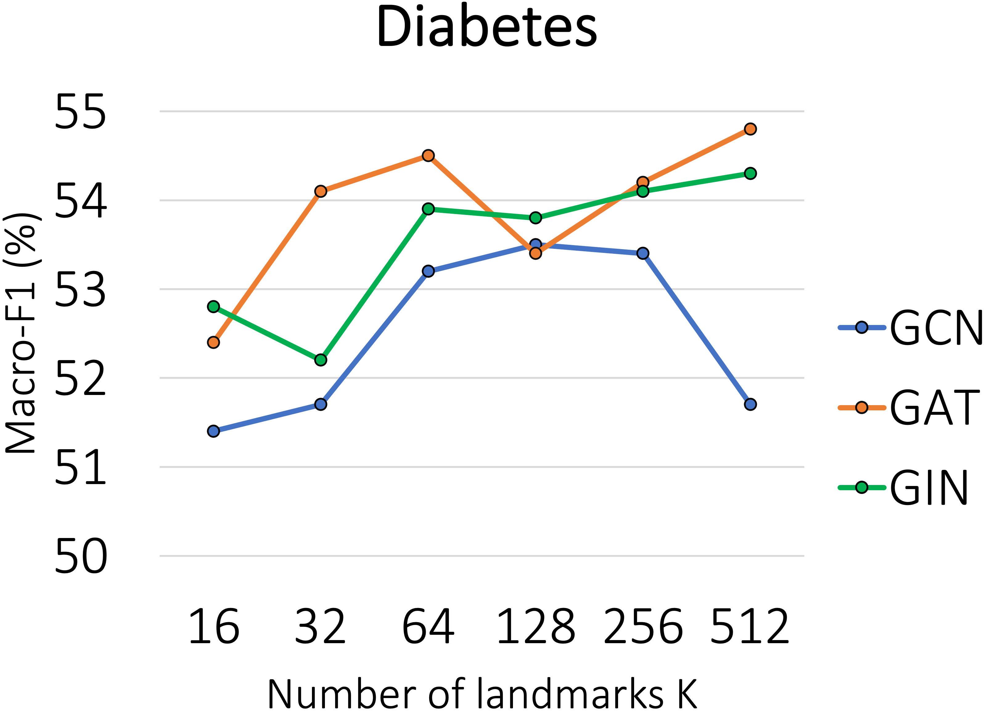
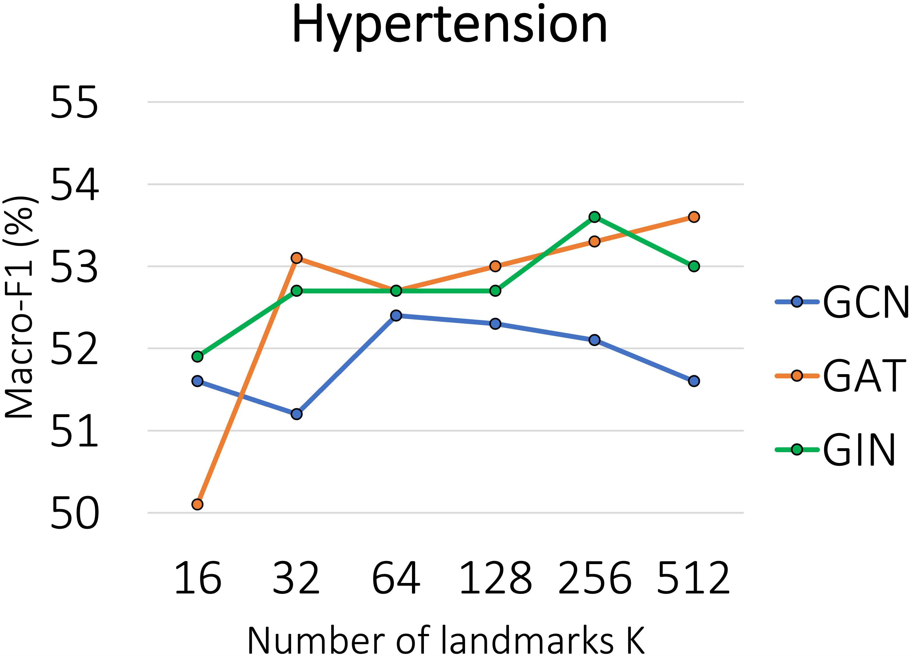
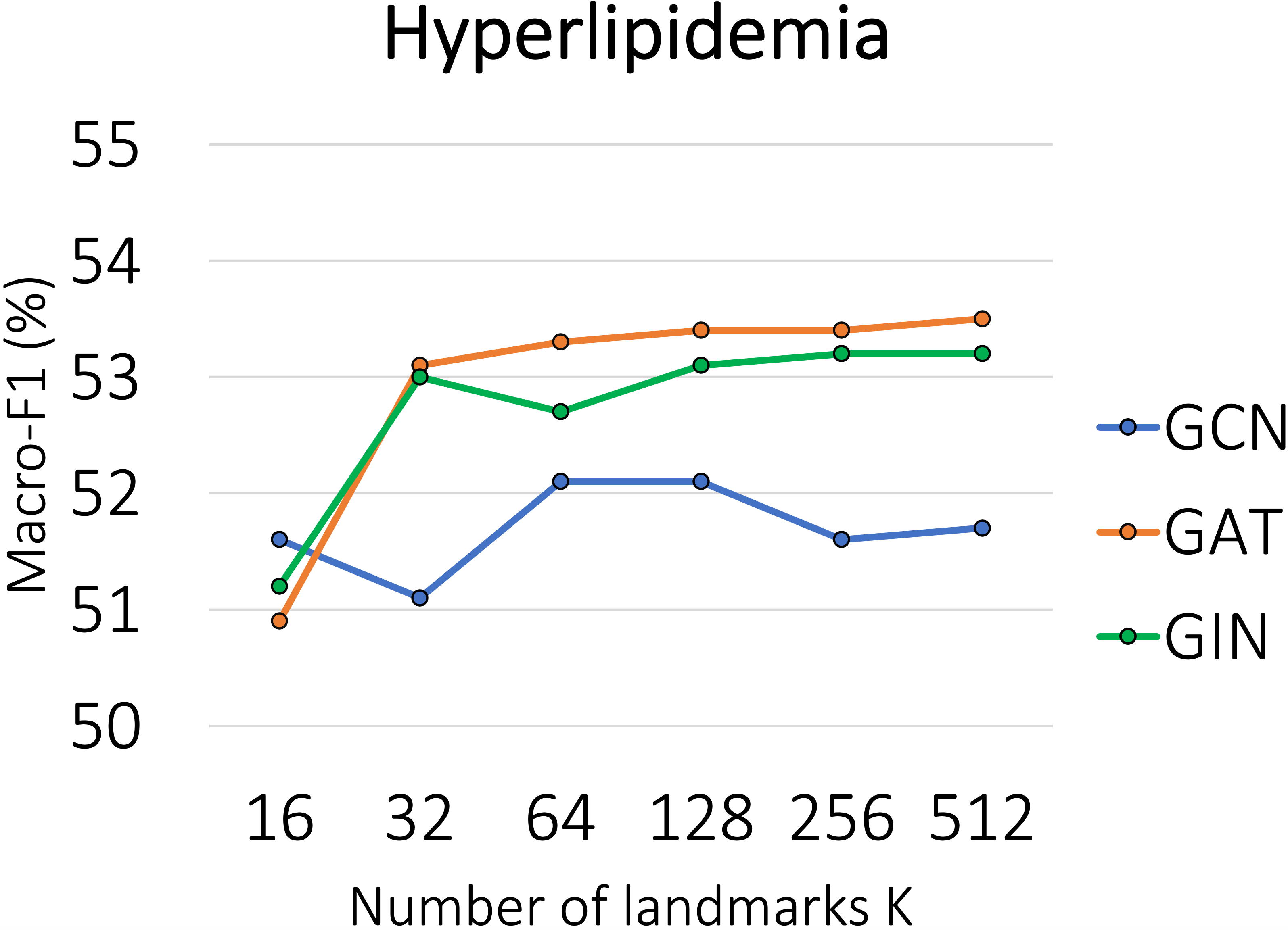
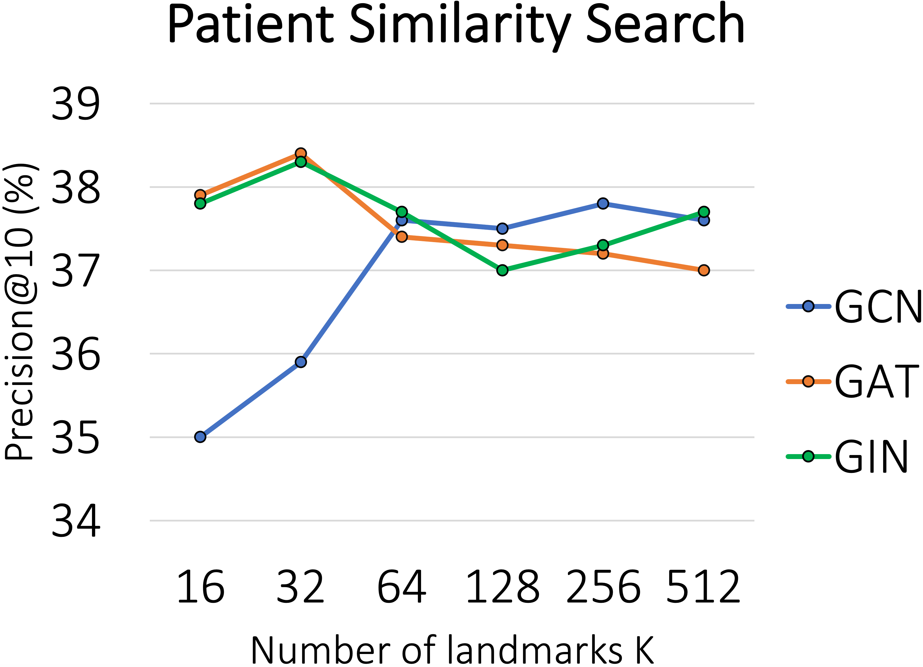
It is common to select different graph encoders to gain better performance on different clinical tasks or diseases. Moreover, the contrastive framework should constantly provide performance boosts for selected graph encoders. Our augmentation scheme is also parameterized by the number of landmarks $K$ selected. This further affects the clustering performance with different $K$. Figure 6 reports the averaged Macro-F1 and Precision@10 of our augmentation framework under different GNNs with different $K$ selection. We can see GAT provides the best overall performance in treatment plan outcome prediction, yet GCN can not produce better results. It is reasonable that the attention mechanism in GAT captures more complex hidden relationships between medical events, as compared to the simple GCN. In general, for the number of landmarks $K$, as $K$ increases, the result improves. However, it is not sensitive to $K$ when performing on patient similarity search. We can see that the precision@10 scores are comparable even when $K$ is small indicating our learning framework can extract as much structural information as possible to sufficiently provide evidence on similarity measure.

Non-Ad Hoc Generalizability in Non-clinical Domains

To see if it is an ad hoc learning framework in the clinical domain, we evaluate GKI on graph classification benchmarks. As in Table 2, GKI generalizes well to other graph classification tasks. Our method outperforms state-of-the-art graph contrastive learning frameworks in 6 out of 8 benchmarks. For lower scores, IMDB-B is the second highest, and RDT-B is still higher than MVGRL and InfoGraph. This gives us an insight that Graph Kernel Informax performs better than those contrastive learning counterparts on clinical applications with the same ability on graph classification benchmarks. This further suggests the generalizability of solving unexplored problems without any prior knowledge.

Figure 7: Comparison of training with and without SVD.

Analysis on Pseudo-inverse

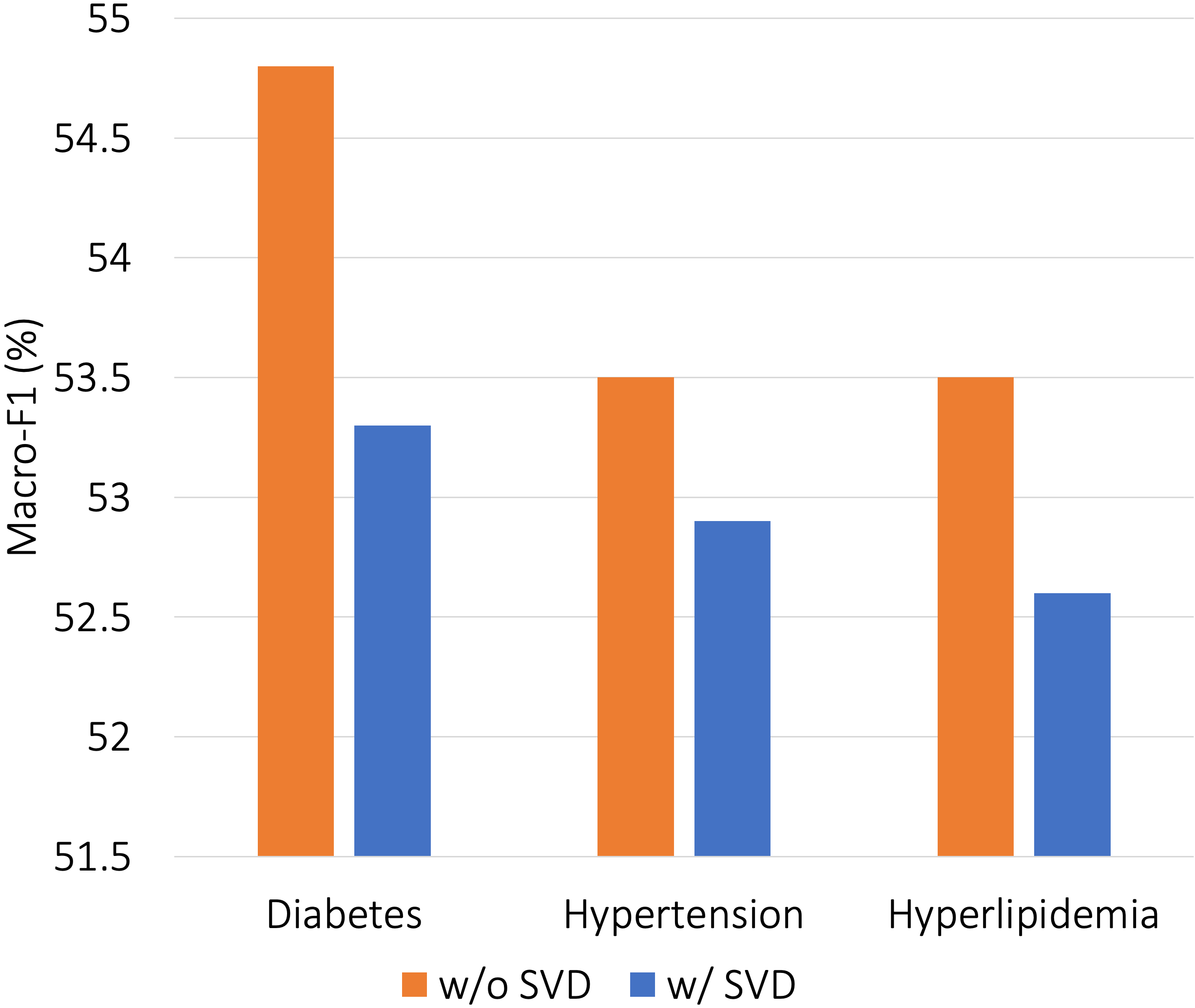
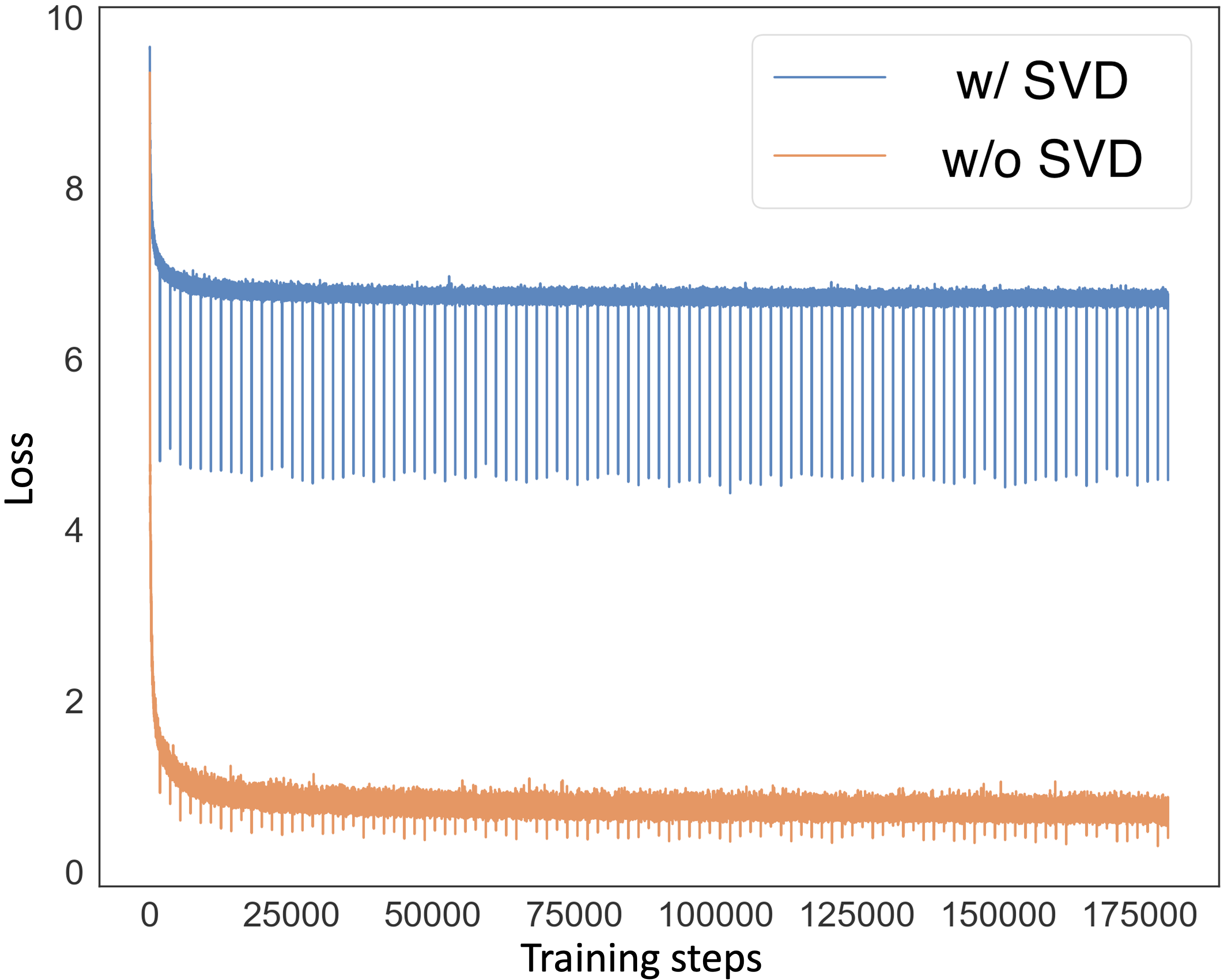
From Figure 7, we notice the performance drop on Macro-F1 on both evaluation scores and convergence when performing Singular Value Decomposition (SVD) during the contrastive learning process. We surmise the reason as SVD defeats the learning signals to the clustering by zeroing out with the singular values associated with each landmark point. Moreover, setting pseudo-inverse to $\mathbin{I}$, which is identical to skipping the SVD step when computing the pseudo-inverse, implicitly defines an orthogonal constraint, since the inverse of the orthogonal matrix is identity. We leave it here for future research.

Conclusion

The complexity of EHR challenges patient representation learning. Many existing efforts addressing such hardship fail to deliver preferable predictive accuracy nor generate highly transferable patient representation for various clinical applications. Consequently, our proposed Graph Kernel Infomax not only overcomes the EHR augmentation problem but also provides a simple and powerful contrastive learning paradigm. We achieve state-of-the-art performance on both clinical application and graph classification benchmarks. Technically, our approach can potentially apply to other domains when graph formulation is determined. Practically, the discussed approach is under limited clinical use and assessment by medical clinicians.

References

- dia (2020) 2020. Introduction: Standards of Medical Care in Diabetes—2020. Diabetes Care.
- Chen et al. (2020) Chen, T.; Kornblith, S.; Norouzi, M.; and Hinton, G. 2020. A simple framework for contrastive learning of visual representations. In International conference on machine learning, 1597–1607. PMLR.
- Choi et al. (2016) Choi, E.; Bahadori, M. T.; Sun, J.; Kulas, J.; Schuetz, A.; and Stewart, W. 2016. Retain: An interpretable predictive model for healthcare using reverse time attention mechanism. In Advances in Neural Information Processing Systems, 3504–3512.
- Choi et al. (2020) Choi, E.; Xu, Z.; Li, Y.; Dusenberry, M.; Flores, G.; Xue, E.; and Dai, A. 2020. Learning the graphical structure of electronic health records with graph convolutional transformer. In Proceedings of the AAAI conference on artificial intelligence, volume 34, 606–613.
- Dong et al. (2017) Dong, Z.; Jia, S.; Zhang, C.; Pei, M.; and Wu, Y. 2017. Deep manifold learning of symmetric positive definite matrices with application to face recognition. In Thirty-First AAAI Conference on Artificial Intelligence.
- Drineas, Mahoney, and Cristianini (2005) Drineas, P.; Mahoney, M. W.; and Cristianini, N. 2005. On the Nyström Method for Approximating a Gram Matrix for Improved Kernel-Based Learning. journal of machine learning research, 6(12).
- Feragen, Lauze, and Hauberg (2015) Feragen, A.; Lauze, F.; and Hauberg, S. 2015. Geodesic exponential kernels: When curvature and linearity conflict. In Proceedings of the IEEE conference on computer vision and pattern recognition, 3032–3042.
- Grundy et al. (2019) Grundy, S. M.; Stone, N. J.; Bailey, A. L.; Beam, C.; Birtcher, K. K.; Blumenthal, R. S.; Braun, L. T.; De Ferranti, S.; Faiella-Tommasino, J.; Forman, D. E.; et al. 2019. 2018 AHA/ACC/AACVPR/AAPA/ABC/ACPM/ADA/AGS/APhA/ASPC/NLA/PCNA guideline on the management of blood cholesterol: executive summary: a report of the American College of Cardiology/American Heart Association Task Force on Clinical Practice Guidelines. Journal of the American College of Cardiology, 73(24): 3168–3209.
- Hassani and Khasahmadi (2020) Hassani, K.; and Khasahmadi, A. H. 2020. Contrastive multi-view representation learning on graphs. In International Conference on Machine Learning, 4116–4126. PMLR.
- He et al. (2015) He, K.; Zhang, X.; Ren, S.; and Sun, J. 2015. Delving deep into rectifiers: Surpassing human-level performance on imagenet classification. In Proceedings of the IEEE international conference on computer vision, 1026–1034.
- Jayasumana et al. (2013) Jayasumana, S.; Hartley, R.; Salzmann, M.; Li, H.; and Harandi, M. 2013. Kernel methods on the Riemannian manifold of symmetric positive definite matrices. In proceedings of the IEEE Conference on Computer Vision and Pattern Recognition, 73–80.
- Johnson et al. (2021) Johnson, A.; Lucas Bulgarelli, T. P.; Steven Horng, L. A. C.; and Mark, R. 2021. MIMIC-IV (version 1.0). PhysioNet.
- Khosla et al. (2020) Khosla, P.; Teterwak, P.; Wang, C.; Sarna, A.; Tian, Y.; Isola, P.; Maschinot, A.; Liu, C.; and Krishnan, D. 2020. Supervised contrastive learning. Advances in Neural Information Processing Systems, 33: 18661–18673.
- Kingma and Ba (2015) Kingma, D. P.; and Ba, J. 2015. Adam: A Method for Stochastic Optimization. In ICLR (Poster).
- Kipf and Welling (2017) Kipf, T. N.; and Welling, M. 2017. Semi-supervised classification with graph convolutional networks. In International Conference on Learning Representations.
- Ko et al. (2022) Ko, C.-Y.; Mohapatra, J.; Liu, S.; Chen, P.-Y.; Daniel, L.; and Weng, L. 2022. Revisiting Contrastive Learning through the Lens of Neighborhood Component Analysis: an Integrated Framework. In International Conference on Machine Learning, 11387–11412. PMLR.
- Li and Dunson (2019) Li, D.; and Dunson, D. B. 2019. Geodesic distance estimation with spherelets. arXiv preprint arXiv:1907.00296.
- Li et al. (2020) Li, Y.; Rao, S.; Solares, J. R. A.; Hassaine, A.; Ramakrishnan, R.; Canoy, D.; Zhu, Y.; Rahimi, K.; and Salimi-Khorshidi, G. 2020. BEHRT: transformer for electronic health records. Scientific reports, 10(1): 1–12.
- Lyu et al. (2018) Lyu, X.; Hueser, M.; Hyland, S. L.; Zerveas, G.; and Raetsch, G. 2018. Improving clinical predictions through unsupervised time series representation learning. arXiv preprint arXiv:1812.00490.
- Ma et al. (2017) Ma, F.; Chitta, R.; Zhou, J.; You, Q.; Sun, T.; and Gao, J. 2017. Dipole: Diagnosis prediction in healthcare via attention-based bidirectional recurrent neural networks. In Proceedings of the 23rd ACM SIGKDD international conference on knowledge discovery and data mining, 1903–1911. ACM.
- Martins and Astudillo (2016) Martins, A.; and Astudillo, R. 2016. From softmax to sparsemax: A sparse model of attention and multi-label classification. In International Conference on Machine Learning, 1614–1623.
- Miotto et al. (2016) Miotto, R.; Li, L.; Kidd, B. A.; and Dudley, J. T. 2016. Deep patient: an unsupervised representation to predict the future of patients from the electronic health records. Scientific reports, 6: 26094.
- Morris et al. (2020) Morris, C.; Kriege, N. M.; Bause, F.; Kersting, K.; Mutzel, P.; and Neumann, M. 2020. TUDataset: A collection of benchmark datasets for learning with graphs. In ICML 2020 Workshop on Graph Representation Learning and Beyond (GRL+ 2020).
- Parimbelli et al. (2018) Parimbelli, E.; Marini, S.; Sacchi, L.; and Bellazzi, R. 2018. Patient similarity for precision medicine: A systematic review. Journal of biomedical informatics, 83: 87–96.
- Qiu et al. (2020) Qiu, J.; Chen, Q.; Dong, Y.; Zhang, J.; Yang, H.; Ding, M.; Wang, K.; and Tang, J. 2020. Gcc: Graph contrastive coding for graph neural network pre-training. In Proceedings of the 26th ACM SIGKDD International Conference on Knowledge Discovery & Data Mining, 1150–1160.
- Shickel et al. (2017) Shickel, B.; Tighe, P. J.; Bihorac, A.; and Rashidi, P. 2017. Deep EHR: a survey of recent advances in deep learning techniques for electronic health record (EHR) analysis. IEEE journal of biomedical and health informatics, 22(5): 1589–1604.
- Sun et al. (2020) Sun, F.-Y.; Hoffman, J.; Verma, V.; and Tang, J. 2020. InfoGraph: Unsupervised and Semi-supervised Graph-Level Representation Learning via Mutual Information Maximization. In International Conference on Learning Representations.
- Unger et al. (2020) Unger, T.; Borghi, C.; Charchar, F.; Khan, N. A.; Poulter, N. R.; Prabhakaran, D.; Ramirez, A.; Schlaich, M.; Stergiou, G. S.; Tomaszewski, M.; et al. 2020. 2020 International Society of Hypertension global hypertension practice guidelines. Hypertension, 75(6): 1334–1357.
- Vedaldi and Zisserman (2012) Vedaldi, A.; and Zisserman, A. 2012. Sparse kernel approximations for efficient classification and detection. In 2012 IEEE Conference on Computer Vision and Pattern Recognition, 2320–2327. IEEE.
- Veličković et al. (2018) Veličković, P.; Cucurull, G.; Casanova, A.; Romero, A.; Liò, P.; and Bengio, Y. 2018. Graph Attention Networks. In International Conference on Learning Representations.
- Velickovic et al. (2019) Velickovic, P.; Fedus, W.; Hamilton, W. L.; Liò, P.; Bengio, Y.; and Hjelm, R. D. 2019. Deep Graph Infomax. ICLR (Poster), 2(3): 4.
- Xu et al. (2018a) Xu, K.; Hu, W.; Leskovec, J.; and Jegelka, S. 2018a. How Powerful are Graph Neural Networks? In International Conference on Learning Representations.
- Xu et al. (2018b) Xu, Y.; Biswal, S.; Deshpande, S. R.; Maher, K. O.; and Sun, J. 2018b. Raim: Recurrent attentive and intensive model of multimodal patient monitoring data. In Proceedings of the 24th ACM SIGKDD international conference on Knowledge Discovery & Data Mining, 2565–2573.
- Yadav et al. (2017) Yadav, P.; Steinbach, M.; Kumar, V.; and Simon, G. 2017. Mining Electronic Health Records: A Survey. ACM Computing Surveys, 50.
- Yang et al. (2017) Yang, B.; Fu, X.; Sidiropoulos, N. D.; and Hong, M. 2017. Towards k-means-friendly spaces: Simultaneous deep learning and clustering. In international conference on machine learning, 3861–3870. PMLR.
- Yang et al. (2022) Yang, H.; Chen, H.; Pan, S.; Li, L.; Yu, P. S.; and Xu, G. 2022. Dual Space Graph Contrastive Learning. arXiv preprint arXiv:2201.07409.
- Yao et al. (2020) Yao, H.-R.; Chang, D.-C.; Frieder, O.; Huang, W.; Liang, I.-C.; and Hung, C.-F. 2020. Cross-global attention graph kernel network prediction of drug prescription. In Proceedings of the 11th ACM International Conference on Bioinformatics, Computational Biology and Health Informatics, 1–10.
- Yèche et al. (2021) Yèche, H.; Dresdner, G.; Locatello, F.; Hüser, M.; and Rätsch, G. 2021. Neighborhood contrastive learning applied to online patient monitoring. In International Conference on Machine Learning, 11964–11974. PMLR.
- You et al. (2020) You, Y.; Chen, T.; Sui, Y.; Chen, T.; Wang, Z.; and Shen, Y. 2020. Graph contrastive learning with augmentations. Advances in Neural Information Processing Systems, 33: 5812–5823.
- Zhang and Kwok (2010) Zhang, K.; and Kwok, J. T. 2010. Clustered Nyström method for large scale manifold learning and dimension reduction. IEEE Transactions on Neural Networks, 21(10): 1576–1587.
- Zhang and Davison (2021) Zhang, Y.; and Davison, B. D. 2021. Deep spherical manifold gaussian kernel for unsupervised domain adaptation. In Proceedings of the IEEE/CVF Conference on Computer Vision and Pattern Recognition, 4443–4452.