Distributional Drift Adaptation with Temporal Conditional Variational Autoencoder for Multivariate Time Series Forecasting

Abstract

Due to the nonstationary nature, the distribution of real-world multivariate time series (MTS) changes over time, which is known as distribution drift. Most existing MTS forecasting models greatly suffer from distribution drift and degrade the forecasting performance over time. Existing methods address distribution drift via adapting to the latest arrived data or self-correcting per the meta knowledge derived from future data. Despite their great success in MTS forecasting, these methods hardly capture the intrinsic distribution changes, especially from a distributional perspective. Accordingly, we propose a novel framework temporal conditional variational autoencoder (TCVAE) to model the dynamic distributional dependencies over time between historical observations and future data in MTSs and infer the dependencies as a temporal conditional distribution to leverage latent variables. Specifically, a novel temporal Hawkes attention mechanism represents temporal factors subsequently fed into feed-forward networks to estimate the prior Gaussian distribution of latent variables. The representation of temporal factors further dynamically adjusts the structures of Transformer-based encoder and decoder to distribution changes by leveraging a gated attention mechanism. Moreover, we introduce conditional continuous normalization flow to transform the prior Gaussian to a complex and form-free distribution to facilitate flexible inference of the temporal conditional distribution. Extensive experiments conducted on six real-world MTS datasets demonstrate the TCVAE’s superior robustness and effectiveness over the state-of-the-art MTS forecasting baselines. We further illustrate the TCVAE applicability through multifaceted case studies and visualization in real-world scenarios.

I Introduction

Multivariate time series (MTS) is a continuous and intermittent unfolding of time-stamped variables over time. MTS forecasting predicts the future values of time-stamped variables based on their extremely substantial historical observations. MTS forecasting is widely applicable for various applications, such as traffic management [1, 2], financial trading [3, 4, 5], energy optimization [6] and epidemic propagation studies [7, 8]. A recent typical example is to predict the case trends of COVID-19 infections, which can provide hints or evidence for intervention policies and prompt actions to contain the virus spread or resurgence and large-scale irreparable socioeconomic impact [9].

Figure 1: An example of MTS traffic flow derived from METR-LA.

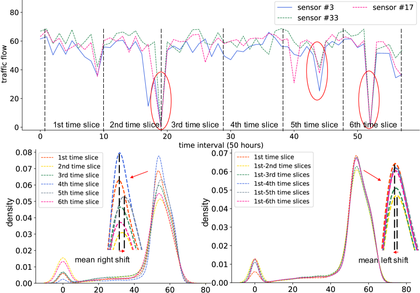
Traditional models such as vector autoregression (VAR) [10] and probabilistic model [11, 12] show appealing interpretability and theoretical guarantees for MTS forecasting. Recent advanced models such as LSTM [13, 14, 15, 16], TCN [17] and Transformer [18, 19] are more competent in capturing temporal dependencies. These models, despite their successful applications in various domains, generally assume that the distribution of time series keeps stationary through time, requiring constant conditional dependencies between future predictions and historical observations. The above assumption oversimplifies the highly nonstationary and non-IID nature of real-world MTSs [20], inapplicable to distribution-evolving MTSs and causing forecasting performance downgrade over time. Such a phenomenon forms distribution drift [21], where the statistical properties of MTSs change over time. As illustrated in Fig. 1, the traffic flows recorded by three sensors $\#$3, $\#$17 and $\#$33 from 9/1/2018 to 12/28/2018 are shown in the upper part, where the flows are split into six successive time slices. The flows sharply descend and ascend, forming the turning points between the 2$nd$ and 3$rd$ slices and within the 5$th$ and 6$th$ slices (marked in red ellipse). In addition, we take out the six slices of sensor $\#$3 and show its statistic evolution in terms of different time slices and cumulative slices in the lower left and right parts, respectively. We can see a mean right shift from the 4$th$ to the 5$th$ slice, as shown in the left part of Fig. 1, and a mean left shift from the 1$st$-2$nd$ time slices to the 1$st$-6$th$ time slices, as shown in the right part of Fig. 1. Obviously, the distribution of successive time series slices changes over time, significantly challenging even well-trained forecasting models. Therefore, addressing MTS distribution drift becomes a critical but challenging issue of MTS forecasting.

Few studies focus on capturing the distribution drift for MTS forecasting to date. Previous methods [22, 23] address the distribution drift via adapting to the latest arrived data and apply the adapted models for future data prediction. However, such methods which hardly capture the intrinsic distribution drift suffer catastrophic forgetting [24] and are unsuitable for scenarios with a sudden distributional change. Subsequently, recent adaptation methods [21, 25, 26] focus on future data and bridge the gaps between historical observations and future data by generating training samples following future data distribution or calculating their gradient difference. These methods learn to correlate the distribution drift with meta knowledge derived from future data and correct the bias caused by their distribution drift in a discriminative meta-learning framework. Despite their great success in MTS forecasting, these methods do not capture significant distribution changes.

Different from previous adaptation-based methods neutralizing the bias caused by the distribution drift, we aim to model the dynamic distributional dependencies over time between historical observations ($\mathcal{X}$) and future data ($\mathcal{Y}$). Inspired by the superiority of generative models, e.g., VAE, in approximating data distribution in various fields [27, 28, 29], we infer the distributional dependencies as a conditional distribution $p(\mathcal{Y}|\mathcal{X})$ by leveraging latent variables $\mathcal{Z}$ in a generative modeling framework. To achieve the dynamics of the conditional distribution over time, we further regularize the latent variables sampled from a prior Gaussian distribution conditional on temporal factors $\mathcal{C}$, i.e., $p(\mathcal{Z}|\mathcal{C})$. As the distributional dependence $p(\mathcal{Y}|\mathcal{X})$ is approximated by the latent variables, it accordingly evolves to a temporal conditional distribution $p(\mathcal{Y}|\mathcal{X},\mathcal{C})$, where the dynamic dependencies between historical observations and future data vary with temporal factors and competently depict the distribution drift.

In light of the above discussion, we propose a novel framework called temporal conditional variational autoencoder (TCVAE) to infer the distributional drift in nonstationary MTSs. TCVAE aims to address three major challenges: (a) accurately approximating the temporal Gaussian distribution $p(\mathcal{Z}|\mathcal{C})$ of the latent variables; (b) dynamically adapting the encoder and decoder structure to distributional changes; (c) flexibly inferring the temporal conditional distribution $p(\mathcal{Y}|\mathcal{X},\mathcal{C})$ from the latent variables. Regarding (a), TCVAE introduces a Hawkes process-based attention mechanism to represent temporal factors and feed-forward networks to learn the mean and derivation of the Gaussian distribution $p(\mathcal{Z}|\mathcal{C})$. Subsequently, the representation of temporal factors is utilized in a gated attention mechanism that adjusts the structures of Transformer-based encoder and decoder in a meta-learning manner to handle (b). Moreover, conditional continuous normalizing flow (CCNF) is exploited to invertibly transform the Gaussian distribution into a complex distribution that is more flexible to infer the temporal conditional distribution to address (c). Our contributions are summarized as follows:

• A temporal conditional variational autoencoder (TCVAE) adapts to distribution drift in MTSs. To our knowledge, TCVAE is the first attempt to depict distribution drift in a generative framework for MTS forecasting.

• A temporal Hawkes attention mechanism represents temporal factors that estimate the temporal Gaussian and a gated attention mechanism dynamically adapts the network structure of the encoder and decoder to distributional changes.

• CCNF is used to transform the temporal Gaussian to a flexible and form-free distribution for effectively inferring the temporal conditional distribution.

Extensive experimental results on six public MTS datasets show the superior robustness and effectiveness of TCVAE over state-of-the-art baselines. Case studies on METR-LA and COVID-19 data further interpret the applicability of TCVAE in real-world environments.

II RELATED WORK

II-A Multivariate Time Series Forecasting

In time series forecasting, traditional statistical models, such as vector autoregression (VAR) [30] and Gaussian process (GP) [31], are simple but interpretable for time series forecasting. However, they make strong assumptions about stationary processes and fall short in capturing non-stationary to non-IID scenarios [20, 32]. Recently, various deep learning models have shown prevalent for MTS forecasting. RNN-based [33, 34, 35] and Transformer-based [18, 19] models are free from the stationary assumptions and are capable of modeling nonlinear long- and short-term temporal patterns. These models pay more attention to capturing the intra-series temporal patterns, but generally neglect the inter-series couplings between multiple variables [32], which weakens their forecasting capacity.

Further, the recent DNN models [36, 37] organize MTSs by a graph with variables being nodes to portray the correlations between variables and graph neural networks (GNNs) to learn the inter-series correlations. GNNs highly depend on a predefined topology structure of inter-series correlations, hence, hardly applicable to MTSs with evolving dependencies and distributional drift. Subsequently, MTGNN [38], AGCRN [1] and StemGNN [8] extract the uni-directed relations among variables and capture shared patterns by graph learning rather than predefined priors. Similarly, CATN [39] introduces a tree (i.e., an ordered graph) to structure multivariable time series with a clear hierarchy and proposes a tree-aware network to learn the hierarchical and grouped correlations among multiple variables. Due to the complex structures of MTSs, it is difficult to learn general graphs, especially for high-dimensional data [40].

Due to the nonstationarity of the real-world environment, distributional drift has been an essential issue in time series data. However, few existing methods focus on the distributional drift of time series. Some strategically cater to future data via adapting their models with the newly arrived data, but they hardly learn the intrinsic distributional drift [22, 23]. In this light, adaptation methods are designed to generate new training samples following future data distribution or calculating gradient differences between historical observations and future data. For example, DDG-DA [21] predicts the evolution of data distribution from a meta-learning perspective through training a predictor to estimate future data distribution and generating corresponding samples for training. TS2VEC [25] uses timestamp masking and random cropping to learn augmented context views for dealing with distributional drifts (level shifts). LLF [26] mitigates the impact of distributional drift via computing the difference between the gradients on historical data and future data. Different from the above methods neutralizing the bias caused by distributional drift, we aim to model the dynamic distributional dependencies between historical observations and future data over time.

II-B Variational Autoencoder

Variational autoencoders (VAEs) as deep generative models are capable of approximating data distribution and have enjoyed great success in various real-world applications, including time series analysis [41, 42, 43], dialog generation [27, 28], text-to-speech [44], recommendation [45] and image processing [46]. In time series analysis, Nguyen et al. [41] introduced a temporal regularization and noise mechanism into a temporal latent autoencoder network to model the predictive distribution of time series implicitly. To well learn the discrete representations of time series, Fortuin et al. [42] overcame the non-differentiability of discrete representations and used a gradient-based self-organizing map algorithm. Dasai et al. [43] relied on the user-defined distribution, such as level, trend, and seasonality, to generate interpretable time series forecasting. Transparently, these models mainly focus on dealing with high-dimensionality and interpretability problems. In addition, based on the robust representation of VAE, conditional VAE regularizes distributional dependencies between historical observations and future data conditional on certain constraints. Inspired by controllable dialog generation [47, 28], we leverage temporal conditional VAE to depict the according dynamic distributional dependencies varying with temporal factors.

II-C Continuous Normalizing Flow

Continuous normalizing flow (CNF) is a continuous version of normalizing flows, which replaces the layer-wise transformations of normalizing flows with ODEs. It is widely used in image/video generation [48, 49], molecular graph generation [50], 3D face recognition [51] and time series forecasting [52]. Luo et al. [50] proposed a discrete latent variable model GraphDF based on CNF methods for molecular graph generation. Zhang et al. [51] learned distributional representation and then transformed this distribution into a flexible form by CNF for low-quality 3D face recognition. These models focus on estimate distribution with a flexible form but conditional constraints need to be considered for capturing complex relationships among variables in reality. For example, given a set of attributes, Abdal et al. [48] devised a CNF-based technique to conditionally resample images with high quality from the GAN latent space. Rasul et al. [52] used a CNF to represent the data distribution in an autoregressive deep learning model. Inspired by these two types of time point modeling processes [51, 48], we design a CCNF to invertibly transform Gaussian distribution into a complex distribution to flexibly represent temporal conditional distribution.

Figure 2: The overall architecture of TCVAE for MTS forecasting. (1) The input $\mathcal{X}$ is first fed into input representation module and ${\rm WE}(\mathcal{X})$ is extracted separately for temporal factor representation; (2) The network details of decoder $\mathcal{T}_{d}$ are similar to encoder $\mathcal{T}_{e}$ with input $\tilde{\bm{{\rm X}}}$ and $\tilde{\bm{{\rm C}}}$; (3) The final loss is a combination of forecasting loss, backcasting loss, and $\mathbb{KL}$ divergence.

III PRELIMINARY

A time series $\bm{{\rm x}}^{i}=\{x_{1}^{i},x_{2}^{i},...,x_{T}^{i}\}$ records the observed values of variable $i$ with $T$ timestamps. A multivariate time series is represented as $\{\bm{{\rm x}}^{1},\bm{{\rm x}}^{2},...,\bm{{\rm x}}^{d_{x}}\ |\ \bm{{\rm x}}^{d_{x}}\in{\mathbb{R}}^{T}\}$, where $d_{x}$ is the variable dimension (the number of univariate time series) and the sampling time interval between two adjacent observed values are constant for all time series.

Problem Statement Under the rolling forecasting setting, given a fixed input time window $w$ and time horizon $h$, we have the historical input of $w$ steps $\mathcal{X}=\{\bm{{\rm x}}^{1},\bm{{\rm x}}^{2},...,\bm{{\rm x}}^{d_{x}}\ |\ \bm{{\rm x}}^{d_{x}}\in{\mathbb{R}}^{w}\}$ at timestamp $T$. Our target is to forecast the future sequence of $h$ steps $\mathcal{Y}=\{\bm{{\rm y}}^{1},\bm{{\rm y}}^{2},...,\bm{{\rm y}}^{d_{y}}\ |\ \bm{{\rm y}}^{d_{y}}\in{\mathbb{R}}^{h}\}$ successive to timestamp $T$, where $d_{y}$ is the variable dimension in forecasting. We reformulate the forecasting target $\mathcal{Y}_{T+h}=\{\bm{{\rm y}}_{T+1},\bm{{\rm y}}_{T+2},...,\bm{{\rm y}}_{T+h}\ |\ \bm{{\rm y}}_{t}\in{\mathbb{R}}^{d_{y}}\}$ along timeline, the input matrix is $\mathcal{X}_{T}=\{\bm{{\rm x}}_{T-w+1},\bm{{\rm x}}_{T-w+2},...,\bm{{\rm x}}_{T}\ |\ \bm{{\rm x}}_{t}\in{\mathbb{R}}^{d_{x}}\}$, where $\mathbf{x}_{t}$ and $\mathbf{y}_{t}$ denote the multivariate values at timestamp $t$ in the historical input and future sequence respectively.

Distributional Drift At timestamp $t$, assume $\mathcal{Y}$ is drawn from a conditional distribution $p(\mathcal{Y}|\mathcal{X})$. In the stationary case, $p(\mathcal{Y}_{t}|\mathcal{X}_{t})$ known by a learning model at timestamp $t$ is applicable to future timestamps; however the time series data generally changes over time, a distributional drift may occur at timestamp $t$, indicating $p(\mathcal{Y}|\mathcal{X})\neq p(\mathcal{Y}_{t}|\mathcal{X}_{t})$.

VAE Architecture VAE gains creativity for its capability of accurately estimating meaningful latent distribution rather than a single data point as in traditional AE. The architecture of VAE consists of an encoder and a decoder. The encoder first encodes the input representation $\bm{{\rm X}}$ to a latent distribution and generates $\bm{{\rm Z}}\in\mathcal{Z}$ obeying this distribution, then the decoder decodes the original input representation $\bm{{\rm X}}$ from $\bm{{\rm Z}}$. The model distribution $p_{\theta}(\bm{{\rm x}})$ is formulated as:

$$p_{\theta}({\bm{{\rm x}}})=\int_{\mathcal{Z}}p_{\theta}(\bm{{\rm x}}|\bm{{\rm z}})p_{\theta}(\bm{{\rm z}})d\mu(\bm{{\rm z}}),\forall\bm{{\rm x}}\in\bm{{\rm X}},\bm{{\rm z}}\in\bm{{\rm Z}}$$ (1)

where $p_{\theta}({\rm z})$ is a prior distribution over the latent $\bm{{\rm Z}}$ and $p_{\theta}(\bm{{\rm x}}|\bm{{\rm z}})$ is the estimated distribution. $\mu(\bm{{\rm z}})$ is the base measure of the latent space $\mathcal{Z}$. With the above architecture, while the encoder gives service to model the posterior distribution $q_{\phi}(\bm{{\rm z}}|\bm{{\rm x}})$, the decoder gives service to approximate the estimated distribution $p_{\theta}(\bm{{\rm x}}|\bm{{\rm z}})$.

IV METHODOLOGY

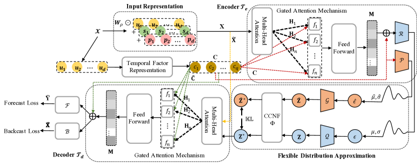
In this section, we propose TCVAE to address the distributional drift problem of MTS forecasting. The overview of the TCVAE architecture is shown in Fig. 2.

IV-A Data Preprocessing

To guarantee the robustness of TCVAE, sequence input $\mathcal{X}\in\mathbb{R}^{T\times d_{x}}$ is normalized and converted to window-sized input $\mathcal{X}\in\mathbb{R}^{w\times d_{x}}$, both for training and testing. Following [17, 1, 39], we perform normalization via $StandardScaler$:

$$\mathcal{X}\leftarrow\frac{\mathcal{X}-\mu(\mathcal{X})}{std(\mathcal{X})+{\epsilon}^{{}^{\prime}}}$$ (2)

where $\mu(\cdot)$ and $std(\cdot)$ calculate the mean and standard deviation vectors respectively. To avoid zero-division, a constant offset ${\epsilon}^{{}^{\prime}}=|\min(\mathcal{X})|$ is required.

IV-B Input Representation

Transformer is used as the skeleton of the encoder ($\mathcal{T}_{e}$) and the decoder ($\mathcal{T}_{d}$) as shown in Fig. 2. Transformer-based models use a self-attention mechanism and timestamps served as local positional context. Intuitively, we regard the distributional drift problem as identifying the shifting context from global information like hierarchical timestamps (A.M. and P.M., day, week, month, year) and agnostic timestamps (holidays, special events). Inspired by [18], we preserve a token embedding and a fixed position embedding, i.e., ${\rm WE}={\rm Conv1d}$, ${\rm PE}_{(pos,2j)}=\sin{(pos/(2w)^{2j/d})}$, ${\rm PE}_{(pos,2j+1)}=\cos{(pos/(2w)^{2j/d})}$, where $d$ is the embedding dimension and $j\in\{1,...,\lfloor d/2\rfloor\}$. ${\rm SE}$ employs $r$ types of global timestamps and maps them into continuous space by one-hot coding. To align the dimension, ${\rm SE}$ projects scalar $\mathcal{X}$ into a $d$-dim matrix. Thus, the embedding function can be formulated as:

$$\bm{{\rm X}}=\bm{W}_{\rho}{\rm WE}(\mathcal{X})+{\rm PE}(\mathcal{X})+{\rm SE}(\mathcal{X})$$ (3)

where $\bm{{\rm X}}\in\mathbb{R}^{w\times d}$ is the embedding output, $\bm{W}_{\rho}$ is a learnable factor matrix balancing the magnitude between the token embedding and position/time embeddings. The embedding outputs from ${\rm WE}$, ${\rm PE}$ and ${\rm SE}$ are extracted as $\{\bm{u}_{1},\bm{u}_{2},...,\bm{u}_{d}\}$, $\{\bm{s}_{1},\bm{s}_{2},...,\bm{s}_{d}\}$ and $\{\bm{p}_{1},\bm{p}_{2},...\bm{p}_{d}\}$, respectively. Let $\bm{{\rm X}}$ and $\bm{\tilde{{\rm X}}}=[\bm{{\rm X}_{t}};\bm{{\rm X}_{0}}]$ denote the inputs of $\mathcal{T}_{e}$ and $\mathcal{T}_{d}$ respectively, where $\bm{{\rm X}_{t}}$ is the start token and $\bm{{\rm X}_{0}}$ is the target sequence which masks the variable values into zero.

IV-C Temporal Factor Representation

Temporal Hawkes Attention In a time slice, the values at each time have different impacts on future values. Therefore, when calculating temporal factor information, we should weigh the critical moments that affect future values [53]. Assume that the current time is $t$, the token embedding $\bm{{\rm U}}=\{\bm{u}_{1},\bm{u}_{2},...,\bm{u}_{d}\}\in\mathbb{R}^{w\times d}$ can be converted to the time axis such as $\bm{u}_{\tau},t-w\leq\tau\leq t-1$. We employ a temporal attention mechanism $\vartheta(\cdot)$ which learns to decide the critical time points (timestamps). This mechanism aggregates temporal features $\bm{{\bar{\rm U}}}=[\bm{u}_{t-w},...,\bm{u}_{t-1}]\in\mathbb{R}^{d\times w}$ from different time points into an overall representation using learned attention weights $\alpha_{\tau}$ for each time point $\tau$. We formulate this mechanism as:

$$\alpha_{\tau}=\frac{exp(\bm{u}_{\tau}^{\mathrm{T}}\bm{W}\bm{{\bar{\rm U}}})}{\sum_{\tau}exp(\bm{u}_{\tau}^{\mathrm{T}}\bm{W}\bm{{\bar{\rm U}}})}$$ (4)

$$\zeta_{\tau}=\alpha_{\tau}\bm{u}_{\tau}$$ (5)

$$\vartheta(\bm{{\bar{\rm U}}})=\sum_{\tau}\zeta_{\tau}$$ (6)

where $\bm{W}$ is a learned linear transform. $\alpha_{\tau}$ denotes the attention weights used to aggregate all temporal features.

The Hawkes process is a self-excited time point process, where the discrete event sequence in continuous time is modeled. Each previous event excites this process to varying degrees. For example, the release of financial policies and crisis information will affect future prices corresponding to varying degrees in the stock market. Although $\vartheta(\bm{{\bar{\rm U}}})$ have captured this complex excitement relationship, the hidden representation cannot well retain the original interpretable factors. Inspired by [3], we propose a temporal Hawkes attention (THA) mechanism to enhance the temporal attention mechanism $\vartheta(\cdot)$ with interpretability by using a Hawkes process. This attention mechanism learns an excitation parameter $\epsilon$ corresponding to time point $\tau$ and a decay parameter $\gamma$ to learn the decay rate of this induced excitement. We compute the temporal features $\bm{{\rm B}}$ as:

$$\bm{{\rm B}}=\sum_{\tau=0,\Delta t_{\tau}\geq 0}(\zeta_{\tau}+\epsilon\max(\zeta_{\tau},0)e^{-\gamma\Delta t_{\tau}})$$ (7)

$\Delta t_{\tau}$ is the time interval between the present and the past time point $\tau$.

Factor Extraction Given the temporal features $\bm{{\rm B}}\in\mathbb{R}^{w\times d}$, we manually construct temporal factors for each time series. Specifically, we obtain the start value $sta$, end value $end$, maximum $max$, minimum $min$, med-value $med$, mean $\mu$ and standard deviation $std$ for each time series and calculate the standard deviation of the means $\mu$ and the standard deviation $std$, i.e., $std({\mu})=std\left({\mu(\bm{{\rm x}}^{i})}_{i=1}^{d_{x}}\right)$ and $std({std})=std\left({std(\bm{{\rm x}}^{i})}_{i=1}^{d_{x}}\right)$ respectively. Accordingly, for each time series, we construct a feature vector of $q$ temporal factors $\{sta,end,max,min,med,\mu,std,std({\mu}),std({std})\}\in\mathbb{R}^{q}$, where $q=9$ is a predefined hyperparameter. Stacking all the feature vectors, we obtain $\bm{{\rm C}}\in\mathbb{R}^{q\times d}$. The temporal factors of $\mathcal{T}_{d}$ are denoted as $\tilde{\bm{{\rm C}}}$, similar to those ($\bm{{\rm C}}$) of $\mathcal{T}_{e}$ as shown in Fig.2.

IV-D Gated Attention Mechanism

We believe that the encoding and decoding process related to prediction should be adapted to distribution changes - as shown in the introduction. Here, the traditional multi-head self-attention of encoder $\mathcal{T}_{e}$ and decoder $\mathcal{T}_{d}$ is briefly introduced. Given each training sample $\bm{{\rm X}}\in\mathbb{R}^{w\times d}$, we perform canonical scaled-dot product attention of the tuple input ($\bm{{\rm Q}}$ (query), $\bm{{\rm K}}$ (key), $\bm{{\rm V}}$ (value)) as $\mathcal{A}(\bm{{\rm Q}},\bm{{\rm K}},\bm{{\rm V}})={\rm Softmax}(\frac{\bm{{\rm Q}}\bm{{\rm K}}^{T}}{\sqrt{d}})\bm{{\rm V}}$, where $d$ is the input representation dimension. The ${\rm Softmax}$ operation shapes the convex combination weights for the values in $\bm{{\rm V}}$, allowing the matrix $\bm{{\rm V}}$ to be compressed into a smaller representative vector for simplified reasoning in the downstream neural network. $\mathcal{A}$ uses a $\sqrt{d}$ term to scale the weights for reducing the variance of the weights. Multi-head self-attention is applied in the form of passing $\bm{{\rm Q}}$, $\bm{{\rm K}}$, $\bm{{\rm V}}$ through $n$ heads and feed-forward layers.

To control the information flow existing in multiple heads adapted to changing temporal factors, we propose a gated attention mechanism (GAM) which extends the above popular scalar attention mechanism by calculating a vector gate instead of a scalar value [54]. The temporal factors is utilized in the vector gate with the soft or hard mode to adjust the structures of encoder and decoder. Let $\bm{{\rm H}}_{i}$ stand for the $i$th head where $i\in\mathbb{Z}^{n}$ and $\mathcal{H}=\{\bm{{\rm H}}_{1},\bm{{\rm H}}_{2},...,\bm{{\rm H}}_{n}\}$. If we have the temporal factors $\bm{{\rm C}}$ in different time slices, the information flow passing through $\bm{{\rm H}}_{i}$ and guided by $\bm{{\rm C}}$ is controlled by gate vector ${\bm{g}}_{i}$ with soft mode as ${\bm{g}}_{i}=\delta(f(\bm{{\rm C}},\bm{{\rm H}}_{i}))$, where $\delta$ represents the element-wise Sigmoid function. However, the $\bm{g}_{i}$ of $\bm{{\rm H}}_{i}$ is also affected by other heads. Inspired by [54, 55], we adapt the gate vector not only on temporal factors and a single head but also on temporal factors and the entire set of heads $\mathcal{H}$, see Fig. 2. To calculate the gate of head $\bm{{\rm H}}_{i}$, each head in the entire set of heads $\mathcal{H}$ and temporal factors will present an individual gate ‘vote’. Then we aggregate the votes to calculate gate ${\bm{g}}_{i}$ for $\bm{{\rm H}}_{i}$. The calculation process of ${\bm{g}}_{i}$ is as follows:

$$\bm{v}^{j}=\bm{W}\bm{{\rm H}}_{j}+\bm{b}$$ (8)

$$\bm{v}^{\bm{{\rm C}}}=\bm{W}\bm{{\rm C}}+\bm{b}$$ (9)

$$s_{i}^{j}=\bm{{\rm H}}_{i}^{T}\bm{v}^{j}$$ (10)

$$s_{i}^{\bm{{\rm C}}}=\bm{{\rm H}}_{i}^{T}\bm{v}^{\bm{{\rm C}}}$$ (11)

$$\beta_{i}^{j}=\frac{\exp(s_{i}^{j})}{\sum_{k\in[1,...,n]}\exp(s_{i}^{k})+\exp(s_{i}^{\bm{{\rm C}}})}$$ (12)

$$\beta_{i}^{\bm{{\rm C}}}=\frac{\exp(s_{i}^{\bm{{\rm C}}})}{\sum_{k\in[1,...,n]}\exp(s_{i}^{k})+\exp(s_{i}^{\bm{{\rm C}}})}$$ (13)

$${\bm{g}}_{i}=f_{i}(\bm{{\rm C}},\bm{{\rm X}})=\delta(\sum_{j}(\beta_{i}^{j}\bm{{\rm H}}_{j})+\beta_{i}^{\bm{{\rm C}}}\bm{{\rm C}})$$ (14)

Here, $\bm{W}$ and $\bm{b}$ are learnable weights and bias shared among functions $f_{1},..f_{n}$. The parameterized function $f$ is more flexible in modeling the interaction between vectors $\bm{{\rm C}}$ and $\bm{{\rm X}}$. Vector $\bm{v}_{j}$ are the output of $\bm{{\rm H}}_{j}$ and $\bm{{\rm C}}$ after linear transformation. $s_{i}^{j}$ is the unnormalized attention score that input $\bm{{\rm H}}_{j}$ put on $\bm{{\rm H}}_{i}$ and $\beta_{i}^{j}$ is the normalized score. The temporal factors are calculated together and the soft weights of $n$ heads are learned. Then we apply to calculate the multi-head self-attention as $\bm{{\rm M}}=[{\bm{g}}_{1},...,{\bm{g}}_{n}]$, where $[\cdot,\cdot]$ denotes a concatenation operation.

IV-E Flexible Distribution Approximation

In MTS forecasting, the forecasting sequence and reconstruction sequence are similar generation processes [44]. The standard VAE generation models assume that the latent variable $\bm{{\rm Z}}$ follows a simple prior distribution such as the Gaussian distribution $\mathcal{N}(\mu,\sigma^{2}I)$ with learnable parameters mean $\mu$ and variance $\sigma^{2}$. To make the training process differentiable, the re-parameterization trick can be adopted:

$$\bm{{\rm Z}}=\mu+\varepsilon\sigma$$ (15)

$$\varepsilon\sim\mathcal{N}(0,I)$$ (16)

However, the latent space is affected by underlying factors over time and becomes increasingly dynamic and complicated to estimate. Motivated by [28], we propose a flexible distribution approximation (FDA) module where the temporal factors are involved in accurately approximating the prior and posterior distribution as shown in Fig. 2. We feed the temporal factors $\bm{{\rm C}}$ and the output $\bm{{\rm M}}$ of the GAM to the process of learning the latent variable. Via transforming random noise $\epsilon$ using neural networks, we sample from the prior Gaussian distribution and posterior distribution over the latent variables. In particular, while the prior sample $\bm{{\hat{\rm Z}}}\sim p_{\theta}(\bm{{\hat{\rm Z}}}|\bm{{\rm C}})$ is produced by a generator $\mathcal{G}$ from temporal$-$dependent random noise $\hat{\epsilon}$, the approximated posterior sample $\bm{{\rm Z}}\sim q_{\phi}(\bm{{\rm Z}}|\bm{{\rm C}},\bm{{\rm M}})$ is produced by a generator $\mathcal{Q}$ from temporal$-$dependent random noise $\epsilon$. $\mathcal{G}$ and $\mathcal{Q}$ are feed-forward neural networks. Both $\hat{\epsilon}$ and $\epsilon$, whose mean covariance matrix are computed from $\bm{{\rm C}}$ with the prior network $\mathcal{P}$ and recognition network $\mathcal{R}$ respectively, are subject to a normal distribution:

$$\left[\begin{array}[]{c}\hat{\mu}\\ \log\hat{\sigma}^{2}\end{array}\right]=\hat{\bm{W}}\mathcal{P}_{\theta}(\bm{{\rm C}})+\hat{\bm{b}}$$ (17)

$$\hat{\epsilon}\sim\mathcal{N}(\epsilon;\hat{\mu},\hat{\sigma}^{2}I)$$ (18)

$$\bm{{\hat{\rm Z}}}=\mathcal{G}_{\theta}(\hat{\epsilon})$$ (19)

$$\left[\begin{array}[]{c}\mu\\ \log{\sigma}^{2}\end{array}\right]=\bm{W}\mathcal{R}_{\phi}(\left[\begin{array}[]{c}\bm{{\rm M}}\\ \bm{{\rm C}}\end{array}\right])+\bm{b}$$ (20)

$$\epsilon\sim\mathcal{N}(\epsilon;\mu,\sigma^{2}I)$$ (21)

$$\bm{{\rm Z}}=\mathcal{Q}_{\phi}(\epsilon)$$ (22)

where $\mathcal{G}_{\theta}(\cdot)$, $\mathcal{P}_{\theta}(\cdot)$, $\mathcal{Q}_{\phi}(\cdot)$ and $\mathcal{R}_{\phi}(\cdot)$ are feed-forward neural networks.

Algorithm 1 The TCVAE training algorithm

0:  window-sized input $\mathcal{X}$, encoder $\mathcal{T}_{e}$, decoder $\mathcal{T}_{d}$, feed-forward networks $\mathcal{G},\mathcal{Q},\mathcal{F},\mathcal{B}$, iteration limit $N$, learning rate $\gamma$

1:  Initialize model parameters $\Theta$

2:  $n\leftarrow 0$

3:  while $n\textless N$ do

4:     $\bm{{\rm X}},\bm{\tilde{{\rm X}}},\bm{{\rm C}},\bm{\tilde{{\rm C}}}\leftarrow\mathcal{X}$ by Equation (2)-(7)

5:     $\mu,\sigma^{2},\hat{\mu},\hat{\sigma}^{2}\leftarrow\mathcal{T}_{e}(\bm{{\rm X}},\bm{{\rm C}})$

6:     $\bm{\hat{{\rm Z}}}\leftarrow\mathcal{G}_{\theta}(\hat{\epsilon})$, $\hat{\epsilon}\leftarrow$ $\hat{\mu},\hat{\sigma}^{2},\epsilon$ by Equation (18), (19)

7:     $\bm{{\rm Z}}\leftarrow\mathcal{Q}_{\phi}(\epsilon),\epsilon\leftarrow\mu,\sigma^{2},\epsilon$ by Equation (21), (22)

8:     Compute the transferred latent variable, i.e. $q(\bm{{\rm Z}}^{\ast}|\bm{{\rm M}},\bm{{\rm C}})$ and $p(\bm{{\hat{\rm Z}}}^{\ast}|\bm{{\rm C}})$ by Equation (25)

9:     $\bm{\hat{{\rm Y}}}\leftarrow\mathcal{F}(\mathcal{T}_{d}(\bm{\tilde{{\rm X}}},\bm{\tilde{{\rm C}}},\bm{{\rm Z}}^{\ast}))$, $\bm{\hat{{\rm X}}}\leftarrow\mathcal{B}(\mathcal{T}_{d}(\bm{\tilde{{\rm X}}},\bm{\tilde{{\rm C}}},\bm{{\rm Z}}^{\ast}))$

10:     Compute the stochastic gradient of $\Theta$ based on $\mathcal{L}(\Theta)$ by Equation (26), (27)

11:     Update $\Theta$ based on the gradients and learning rate $\gamma$

12:     $n\leftarrow n+1$

13:  end while

Conditional Continuous Normalizing Flow The posterior distribution $q(\bm{{\rm Z}}|\bm{{\rm M}},\bm{{\rm C}})$ is intractable but usually approximated by Gaussian distribution. Nevertheless, it is unrealistic to think of the posterior as Gaussian distribution. Regardless of the family of distributions we choose to estimate the posterior, it may not fit. Inspired by [51], we use CCNF to invertibly transform the Gaussian distribution into a complex distribution for flexibly inferring the temporal conditional distribution. First, a latent variable obeys a Gaussian distribution $\mathcal{N}(\mu,\sigma)$. A CCNF ${\Phi}$ is then used to convert the sample of this Gaussian distribution. After applying a continuous-time dynamics, the latent variable $\bm{{\rm Z}}^{\ast}\in\mathbb{R}^{w\times k}$, where $k$ denotes the representation dimension of the latent variable, is computed as follows:

$$\bm{{\rm Z}}^{\ast}=\Phi(\bm{{\rm Z}}(t_{0}))=\bm{{\rm Z}}(t_{0})+\int_{t_{0}}^{t_{1}}\Omega(\bm{{\rm Z}}(t),t)dt$$ (23)

$$\bm{{\rm Z}}(t_{0})\sim\mathcal{N}(\mu,\sigma)$$ (24)

where $\bm{{\rm Z}}=\bm{{\rm Z}}(t_{0})$, $\bm{{\rm Z}}^{\ast}=\bm{{\rm Z}}(t_{1})$, and $\Omega$ is a continuous mapping as $\Omega(\bm{{\rm Z}}(t),t)=\frac{\partial\bm{{\rm Z}}(t)}{\partial t}$ with the initial value $\bm{{\rm Z}}(t_{0})=\bm{{\rm Z}}_{0}$. Therefore, the log-density of the transferred latent variable is:

$$\log q(\bm{{\rm Z}}^{\ast}|\bm{{\rm M}},\bm{{\rm C}})=\log q(\bm{{\rm Z}}(t_{0})|\bm{{\rm M}},\bm{{\rm C}})-\int_{t_{0}}^{t_{1}}{\rm Tr}(\frac{\partial\Omega}{\partial\bm{{\rm Z}}(t)})dt$$ (25)

By this means, the Gaussian distribution is turned into a form-free posterior. The same operation is also performed on $\bm{{\hat{\rm Z}}}$ to obtain $\bm{{\hat{\rm Z}}}^{\ast}$. This transformation facilitates our model to learn a more flexible distribution $p(\bm{{\hat{\rm Z}}}^{\ast}|\bm{{\rm C}})$ and $q(\bm{{\rm Z}}^{\ast}|\bm{{\rm M}},\bm{{\rm C}})$. CCNF can potentially learn a less entangled internal representation.

IV-F Learning Objective

We input the flexible posterior distribution $q(\bm{{\rm Z}}^{\ast}|\bm{{\rm M}},\bm{{\rm C}})$, temporal factors $\tilde{\bm{{\rm C}}}$ and input representation $\tilde{\bm{{\rm X}}}$ together into decoder $\mathcal{T}_{d}$ for decoding. The decoding results flow to the backcasting network $\mathcal{B}$ and the forecasting network $\mathcal{F}$ and generate outputs denoted by $\bm{\hat{{\rm X}}}$ and $\bm{\hat{{\rm Y}}}$, respectively. Given the generated waveform $\bm{\hat{{\rm X}}}$ and $\bm{\hat{{\rm Y}}}$, we thus want to maximize the variational lower bound, also alluded to as the evidence lower bound (ELBO):

$$\begin{split}\max\limits_{\theta,\phi,\psi,\Upsilon}&\mathbb{E}_{q_{\phi}(\bm{{\rm Z}}^{\ast}|\bm{{\rm M}},\bm{{\rm C}})}\log p_{\psi}(\bm{\hat{{\rm X}}}|\bm{{\rm Z}}^{\ast},\tilde{\bm{{\rm C}}},\tilde{\bm{{\rm X}}})+\mathbb{E}_{q_{\phi}(\bm{{\rm Z}}^{\ast}|\bm{{\rm M}},\bm{{\rm C}})}\\ &\log p_{\Upsilon}(\bm{\hat{{\rm Y}}}|\bm{{\rm Z}}^{\ast},\tilde{\bm{{\rm C}}},\tilde{\bm{{\rm X}}})-\lambda\mathbb{KL}(q_{\phi}(\bm{{\rm Z}}^{\ast}|\bm{{\rm M}},\bm{{\rm C}})||p_{\theta}(\bm{{\hat{\rm Z}}}^{\ast}|\bm{{\rm C}}))\end{split}$$ (26)

$$\begin{split}&\mathbb{KL}(q_{\phi}(\bm{{\rm Z}}^{\ast}|\bm{{\rm M}},\bm{{\rm C}})||p_{\theta}(\bm{{\hat{\rm Z}}}^{\ast}|\bm{{\rm C}}))\\ &=\mathbb{E}_{q_{\phi}(\bm{{\rm Z}}^{\ast}|\bm{{\rm M}},\bm{{\rm C}})}\log q_{\phi}(\bm{{\rm Z}}^{\ast}|\bm{{\rm M}},\bm{{\rm C}})-\mathbb{E}_{p_{\theta}(\bm{{\hat{\rm Z}}}^{\ast}|\bm{{\rm C}})}\log p_{\theta}(\bm{{\hat{\rm Z}}}^{\ast}|\bm{{\rm C}})\\ &=\mathbb{E}_{q_{\phi}(\bm{{\rm Z}}^{\ast}|\bm{{\rm M}},\bm{{\rm C}})}[\frac{{\bm{{\rm Z}}^{\ast}}^{2}}{2}-\int_{t_{0}}^{t_{1}}{\rm Tr}(\frac{\partial\Omega}{\partial\bm{{\rm Z}}(t)})dt]\\ &\qquad-\mathbb{E}_{p_{\theta}(\bm{{\hat{\rm Z}}}^{\ast}|\bm{{\rm C}})}[\frac{{\bm{{\hat{\rm Z}}}^{\ast}}^{2}}{2}-\int_{t_{0}}^{t_{1}}{\rm Tr}(\frac{\partial\Omega}{\partial\bm{{\hat{\rm Z}}}(t)})dt]\end{split}$$ (27)

where $p_{\theta}(\bm{{\hat{\rm Z}}}^{\ast}|\bm{{\rm C}})$ and $q_{\phi}(\bm{{\rm Z}}^{\ast}|\bm{{\rm M}},\bm{{\rm C}})$ are neural networks implementing Equations (17)-(25). $p(\bm{{\hat{\rm Z}}}^{\ast}|\bm{{\rm C}})$ is the prior distribution given condition $\bm{{\rm C}}$. $p_{\psi}(\bm{\hat{{\rm X}}}|\bm{{\rm Z}}^{\ast},\tilde{\bm{{\rm C}}},\tilde{\bm{{\rm X}}})$ is the integration of decoder $\mathcal{T}_{d}$ and backcasting network $\mathcal{B}$. $p_{\Upsilon}(\bm{\hat{{\rm Y}}}|\bm{{\rm Z}}^{\ast},\tilde{\bm{{\rm C}}},\tilde{\bm{{\rm X}}})$ is the integration of decoder $\mathcal{T}_{d}$ and forecasting network $\mathcal{F}$. $\lambda$ is a trade-off parameter.

The pseudo-code for the overall training process is summarized in Algorithm 1. We aim at minimizing the training loss $\mathcal{L}(\Theta)$, i.e., the negative ELBO that can be considered as the sum of reconstruction loss $-\log p_{\psi}(\bm{\hat{{\rm X}}}|\bm{{\rm Z}}^{\ast},\tilde{\bm{{\rm C}}},\tilde{\bm{{\rm X}}})$, forecasting loss $-\log p_{\psi}(\bm{\hat{{\rm Y}}}|\bm{{\rm Z}}^{\ast},\tilde{\bm{{\rm C}}},\tilde{\bm{{\rm X}}})$ and Kullback-Leibler $\mathbb{KL}$ divergence $q_{\phi}(\bm{{\rm Z}}^{\ast}|\bm{{\rm M}},\bm{{\rm C}})||p_{\theta}(\bm{{\hat{\rm Z}}}^{\ast}|\bm{{\rm C}})$. $\Theta$ is the model parameter and we set the loss weight for all experiments.

TABLE I: Dataset statistics.

Datasets	Samples	Variables	Sample interval	Start time
Traffic	10,392	963	1 hour	1/1/2008
Electricity	25,968	370	1 hour	1/1/2012
Solar-Energy	52,560	137	10 minutes	1/1/2016
COVID-19	674	280	1 day	1/22/2020
PeMsD7(M)	11,232	228	5 minutes	7/1/2016
METR-LA	34,272	207	5 minutes	9/1/2018

TABLE II: Overall comparison of different methods on six datasets with $w=24,h=24$, where the best results are highlighted in bold and the suboptimal results are underlined (smaller value indicates better performance). Note that we report parts of the results due to the page limitation.

Datasets	Metrics	Models
		LSTNet	DSANet	DeepGLO	Informer	StemGNN	AGCRN	STNorm	TS2VEC	TCVAE
Traffic	MAE	0.0221	0.0256	0.0237	0.0433	0.0376	0.0139	0.0153	0.013	0.0127
	RMSE	0.0504	0.048	0.024	0.0713	0.0653	0.0277	0.0287	0.025	0.0236
	MAPE	0.3673	0.1962	0.3207	0.2061	0.5632	0.1183	0.1305	0.1106	0.1071
Electricity	MAE	0.0676	0.0734	0.0758	0.0701	0.0887	0.0363	0.0377	0.0353	0.034
	RMSE	0.1311	0.267	0.2841	0.1248	0.1404	0.2568	0.1374	0.152	0.1167
	MAPE	1.0979	0.2451	0.2094	0.3295	0.3453	0.1013	0.1236	0.1088	0.1094
Solar-Energy	MAE	0.1533	0.2148	0.1608	0.0693	0.18	0.1378	0.1432	0.162	0.1375
	RMSE	0.2972	0.3996	0.3586	0.1241	0.3696	0.355	0.2947	0.3345	0.2752
	MAPE	0.1008	0.0781	0.0806	0.0736	0.07	0.0576	0.066	0.0638	0.054
COVID-19	MAE	0.1325	0.0786	0.0837	0.118	0.1122	0.0595	0.0958	0.058	0.0524
	RMSE	0.3618	0.2159	0.1743	0.2913	0.1444	0.3189	0.2703	0.1749	0.1041
	MAPE	3.0203	4.5795	3.4002	2.4193	3.3537	1.8096	1.1439	3.4108	1.9812
PeMSD7(M)	WAPE	0.1806	0.0984	0.1085	0.0993	0.0758	0.059	0.0579	0.0663	0.0573
	MAPE	0.3321	0.0994	0.1791	0.1951	0.0966	0.0654	0.0685	0.0708	0.0612
	SMAPE	0.2261	0.0904	0.1301	0.1381	0.0845	0.0304	0.0689	0.0582	0.0591
METR-LA	WAPE	0.2412	0.0965	0.1186	0.102	0.0591	0.1242	0.0652	0.0553	0.0542
	MAPE	0.2852	0.0986	0.1452	0.1135	0.0732	0.1199	0.0672	0.0657	0.0641
	SMAPE	0.216	0.101	0.0761	0.0735	0.0619	0.0574	0.068	0.0602	0.0581

TABLE III: Overall accuracy on Traffic and Solar-Energy with $w=24,h=\{48,72,96\}$, where the best performance is highlighted in bold.

Datasets	Methods	$h=48$			$h=72$			$h=96$
		MAE	RMSE	MAPE	MAE	RMSE	MAPE	MAE	RMSE	MAPE
Traffic	AGCRN	0.0143	0.0281	0.1209	0.0143	0.0284	0.1229	OOM	OOM	OOM
	STNorm	0.0174	0.0335	0.1576	0.0156	0.0303	0.1339	0.02	0.036	0.1811
	TS2VEC	0.0128	0.0258	0.123	0.0143	0.025	0.1206	0.0171	0.0281	0.1317
	TCVAE	0.0142	0.0247	0.109	0.0142	0.0248	0.1222	0.0151	0.0269	0.1299
Solar-Energy	AGCRN	0.1757	0.3964	0.07	0.1971	0.432	0.0763	0.2068	0.4437	0.0791
	STNorm	0.1771	0.357	0.0706	0.2022	0.4131	0.0816	0.2324	0.4403	0.0838
	TS2VEC	0.201	0.3864	0.0786	0.2113	0.401	0.0827	0.212	0.4021	0.083
	TCVAE	0.1747	0.3523	0.0693	0.192	0.3985	0.0761	0.2084	0.435	0.0822

V EXPERIMENTS

V-A Datasets and Metrics

Six public multivariate time series datasets are used in the experiments and summarized in Table I.

Traffic It records the hourly occupancy rate of different lanes on San Francisco highway from 1/1/2008 to 3/30/2009 and contains 10,392 timestamps and 963 sensors.

Electricity It collects the hourly electricity consumption of 370 clients and involves 25,968 timestamps.

Solar-Energy It collects the solar power production records every $10$ minutes from 137 PV plants in Alabama State in 2007 and includes 52,560 timestamps.

COVID-19 The dataset records the daily number of newly confirmed cases from 1/22/2020 to 11/25/2021 collected from the COVID-19 Data Repository.

PeMSD7(M) It is from the sensors spanning the freeway system of California and consists of 11,232 timestamps and 228 variables at a 5-minute interval.

METR-LA The dataset records traffic information from 207 sensors of the Los Angeles County’s highway. It contains 34,272 timestamps and 207 variables at a 5-minute interval.

Following previous works [39, 17], we evaluate all comparative methods via six metrics: Mean Absolute Error $MAE=\frac{1}{N}\sum_{i=1}^{N}\left|\bm{{\rm y}}_{i}-\hat{\bm{{\rm y}}}_{i}\right|$, Root Mean Squared Error $RMSE=\sqrt{\frac{1}{N}\sum_{i=1}^{N}(\bm{{\rm y}}_{i}-\hat{\bm{{\rm y}}}_{i})^{2}}$, Mean Absolute Percent Error $MAPE=\frac{1}{N}\sum_{i=1}^{N}\frac{\left|\bm{{\rm y}}_{i}-\hat{\bm{{\rm y}}}_{i}\right|}{\bm{{\rm y}}_{i}}\mathds{1}\{\left|\bm{{\rm y}}_{i}\right|>0\}$, Symmetric Mean Absolute Percent Error $SMAPE=\frac{1}{N}\sum_{i=1}^{N}\frac{\left|\bm{{\rm y}}_{i}-\hat{\bm{{\rm y}}}_{i}\right|}{\left|\bm{{\rm y}}_{i}+\hat{\bm{{\rm y}}}_{i}\right|/2}\mathds{1}\{\left|\bm{{\rm y}}_{i}\right|>0\}$ and Weighted Absolute Percent Error $WAPE=\frac{\sum_{i=1}^{N}\left|\bm{{\rm y}}_{i}-\hat{\bm{{\rm y}}}_{i}\right|}{\sum_{i=1}^{N}\left|\bm{{\rm y}}_{i}\right|}$, where $N$ denotes the number of samples in the testing set, $\hat{\bm{{\rm y}}}_{i}$ and $\bm{{\rm y}}_{i}$ denote the prediction and groundtruth respectively.

V-B Baselines

We compare our TCVAE with the following state-of-the-art multivariate time series forecasting baselines. All baselines adopt the same normalization method as TCVAE.

(1) LSTNet [13]: It employs two key components including a convolutional neural network and an LSTM with recurrent-skip connection in the time dimension;

(2) DSANet [34]: It constructs global and local temporal convolution to extract complicated temporal patterns and employs self-attention to model dependencies;

(3) DeepGLO [17]: It is a TCN-based model that can focus on both global and local features;

(4) Informer [18]: It is a Transformer-like architecture with a sparse-attention mechanism to maintain a higher capacity for long sequence prediction;

(5) StemGNN [8]: It uses a graph network to capture inter-series and intra-series correlation jointly in the spectral domain;

(6) AGCRN [1]: It has a graph-learning component and a personalized RNN component to extract fine-grained spatial and temporal correlations automatically;

(7) STNorm [56]: It employs temporal and spatial normalization modules which separately refine the local component and the high-frequency component underlying the raw data. We use the version with Wavenet as the backbone;

(8) TS2VEC [25]: It focuses on using timestamp masking and random cropping to learn augmented context views for dealing with level shifts of time series data.

V-C Implementation Details and Settings

Following the commonly-used settings in [2, 1], we predict future $h=24$ timestamps (1 day/4 hours) using historical $w=24$ timestamps (1 day/4 hours). Additionally, we increase the prediction timestamps to $h=48$ (2 days/8 hours), $h=72$ (3 days/12 hours) and $h=96$ (4 days/16 hours) on Traffic and Solar-Energy datasets respectively to investigate the performance of long-term forecasting. We use an Adam optimizer with a fixed learning rate of 0.001, a batch size of 64, and epochs of 50 to train our model. In addition, we elaborately tune the hyperparameters and select the settings with best performance: specifically, the trade-off parameter $\lambda\in\{1,10^{-1},10^{-2},10^{-3}\}$, the number of heads $n\in\{4,8,16\}$, the representation dimension $d\in\{256,512,1024\}$ and the latent variable dimension $k\in\{256,512,1024\}$. When training on Electricity, $\lambda$ is set to 0.01 and otherwise, $\lambda$ is set to 0.1. Regarding to the rolling step, we consider a commonly-used setting [18, 41, 39] for a multi-step forecasting setup that the rolling step is fixed to 1. In the parameter sensitivity experiment, the window size $w$ is selected from $\{12,24,32\}$. We implement TCVAE and other baselines on Python 3.6.13 with the package Pytorch 1.8.1. The codes of our model and baselines are carried out on Ubuntu 18.04.6 LTS, with one Inter(R) Xeon(R) CPU @ 2.10GHz and four NVIDIA GeForce 3090 GPU cards.

V-D Results

V-D1 Overall Comparison

Table II shows the overall experimental results on the default forecasting setup of $w=24$ and $h=24$, where we adopt five widely used metrics: MAE, RMSE, MAPE, WAPE and SMAPE, to measure the performance of the comparative models. Remarkably, TCVAE establishes a new state-of-the-art on most of the datasets and obtains an average improvement of 7.7$\%$ on MAE, 21.8$\%$ on RMSE, 12.7$\%$ on MAPE, 7.8$\%$ on WAPE and 2.5$\%$ on SMAPE compared with the best baseline TS2VEC on the datasets. Regarding the baseline models, the temporal-aware models, i.e., LSTNet, DSANet, DeepGLO, and Informer, focus on capturing temporal information through combining the sequential models, e.g., RNN or Transformer, and attention mechanism and achieve desirable performance. Especially, Informer, a state-of-the-art deep learning model, achieves appreciable performance on Solar-Energy and Electricity. Compared with the temporal-aware models, the GNN-based models StemGNN, AGCRN, and STNorm can capture dynamic correlations explicitly among multiple time series and show better performance. For example, AGCRN shows competitive performance on several datasets, e.g., PeMSD7(M) and METR-LA. This is because the models use parallel parameter space for time series to model temporal and topology dynamics jointly without a need for a predefined structure. However, the GNN-based models, especially AGCRN, require higher memory space compared with other models when dealing with high-dimensional data such as Traffic (963 dimensions). In addition, the above GNN-based models have performance limitations and fall behind TS2VEC and our proposed TCVAE, this is attributed to the fact that the distributions of adjacent time slices are diverse and change over time (level drifts). TS2VEC tackles the issue via leveraging timestamp masking and random cropping to deal with distributional drifts and achieves impressive performance second to TCVAE. From all the results, we conclude that, in addition to capturing temporal information and inter-series correlations, using temporal factors to guide distributional drift learning is important and effective.

TABLE IV: Results of ablation study on the Electricity dataset.

Metrics	MAE	RMSE	MAPE	SMAPE
w/o THA	0.0446	0.1588	0.1483	0.1611
w/o GAM	0.0505	0.1606	0.1884	0.2204
w/o FDA	0.0488	0.1225	0.1963	0.2286
w/o $\mathbb{KL}$	0.0615	0.1495	0.2803	0.3015
w/o Backcasting	0.045	0.1477	0.1616	0.1688
TCVAE	0.034	0.1167	0.1094	0.1114

To investigate the ability of the comparative models in long sequence forecasting, we further conduct experiments via fixing $w=24$ and enlarging $h$ to 48, 72, and 96. The experimental results are shown in Table III. We only compare TCVAE with AGCRN, STNorm, and TS2VEC, which are the top-3 baselines from the above experiments. From the results, we can observe that TCVAE outperforms the baselines significantly, indicating the superiority of TCVAE in long sequence forecasting over the baselines. It is worth noting that AGCRN highly benefits from modeling intra-series correlations within a topological structure and achieves better performance than TCVAE on Solar-Energy with $h=96$. This may be attributed to the fact that long time series facilitates a more accurate learned structure but brings extreme challenges for learning distributional drifts. However, when the number of variables is large, e.g., on Traffic, AGCRN with the representation dimension of nodes being 10 runs out of memory (as marked in OOM in Table III). In contrast, TCVAE functions well on Traffic, further indicating the high scalability of TCVAE, relative to GNN-based models, especially AGCRN.

V-D2 Ablation Study

To better understand the effectiveness of different components in TCVAE, we perform additional experiments on the Electricity dataset with ablation consideration by removing different components from TCVAE. We select a setting as $w=24$ and $h=24$ in the experiments. Table IV summarizes the results and shows that all the components are integral. Specifically, w/o THA is a variant where $b_{t}$ is removed from TCVAE, and its temporal factor representation focuses on global-location rather than local-location contribution. Comparing TCVAE and w/o THA, we observe that temporal Hawkes attention significantly improves temporal attention, verifying our design of using the Hawkes process to model time series as temporal point processes. TCVAE shows significant improvement (+32.7$\%$, +27.3$\%$, +41.9$\%$, +49.5$\%$ corresponding to MAE, RMSE, MAPE, and SMAPE respectively) over variant w/o GAM, verifying the effect of temporal factors in guiding the generation of information flow. In addition, the superiority of TCVAE over variant w/o FDA using a standard CVAE and removing CCNF ${\Phi}$ indicates that breaking the specific distribution form is of great significance. And the improvement of TCVAE over variants w/o Backcasting and w/o $\mathbb{KL}$ proves that both temporal conditions and backcasting designs can introduce additional information and improve sequence representation capacity. Back to Table IV, the MAE, RMSE, MAPE and SMAPE of TCVAE are significantly improved (+44.7$\%$, +21.9$\%$, +61.0$\%$, +63.1$\%$) over w/o $\mathbb{KL}$. We note that removing backcasting in variant w/o Backcasting does not lead to significant degradation in performance, probably because the backcasting (reconstruction) loss has the same or duplicated effect as the forecasting loss.

(a) Effect of window size $w$

(b) Effect of trade-off parameter $\lambda$

(c) Effect of number of heads $n$

(d) Effect of representation dimension $d$

Figure 3: Parameters sensitivity analysis of TCVAE on MAE and MAPE.

V-D3 Parameter Sensitivity

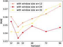
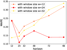
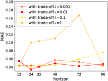
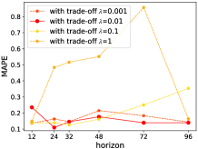
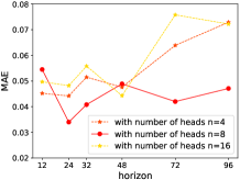
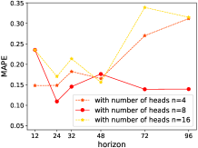
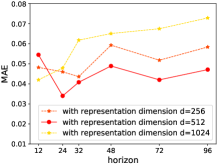
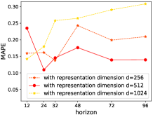
We investigate the sensitivity of TCVAE in terms of the time window size $w\in\{24,32,64\}$, the trade-off parameter $\lambda\in\{1,10^{-1},10^{-2},10^{-3}\}$, the number of heads $n\in\{4,8,16\}$, the representation dimension $d\in\{256,512,1024\}$ and the latent variables dimension $k\in\{256,512,1024\}$ on Electricity. Fig. 3 (a) - (d) shows the MAE and MAPE on Electricity by changing one parameter while fixing others. From the results, we have observations as follows. (1) Window size $w$: Window size impacts learning distributional drifts. When predicting a short horizon (such as $h=12$), initially increasing window size degrades the performance. When $h\textgreater 72$, $w=24$ achieves the best performance. The interpretation from a training perspective is that a relatively small value of $w$ may not pass enough information to the latent space $\mathcal{Z}$, while a large value of $w$ brings redundant information leading to losing accuracy. (2) Trade-off parameter $\lambda$: The influence of weight $\lambda$ for the $\mathbb{KL}$ loss term (Equation (26)) is analyzed. The setting $\lambda=0.01$ on Electricity and $\lambda=0.1$ on other datasets (not shown in Fig. 3) give the optimal results. The results confirm that: a larger $\lambda$ imposes a stronger emphasis on VAE to find the underlying factors leading to drift; however, a large $\lambda$ (e.g., $\lambda=1$) may hurt the performance. (3) Number of heads $n$: The results report that 4-head attention achieves the best performance in predicting 12 timestamps. The forecasting quality drops off with too many heads $n=16$. (4) Representation dimension $d$: The representation dimension of inputs and temporal factors in TCVAE highly determines the parameter effectiveness in temporal factor guidance and the capability of the learned representations. Fig. 3 (d) shows the impact of various representation dimensions on Electricity. When the representation dimension is set to 512, TCVAE achieves the best performance. An excessively small or large representation dimension will result in poor performance. (5) Latent variable dimension $k$: As shown in Table V, similar to the representation dimension, $k=512$ results in the best performance of TCVAE, confirming that larger $k$ improves the representation capability of TCVAE but may easily lead to the overfitting problem.

TABLE V: Effect of different latent variable dimensions.

k	MAE	RMSE	MAPE	SMAPE
256	0.0489	0.163	0.1735	0.1988
512	0.034	0.1167	0.1094	0.1114
1024	0.0455	0.1565	0.1579	0.1749

V-D4 Case Study

We deliver some case examples and explain the learned pattern of TCVAE. Traffic and pandemic data are highly dynamic and volatile, providing excellent scenarios for case studies.

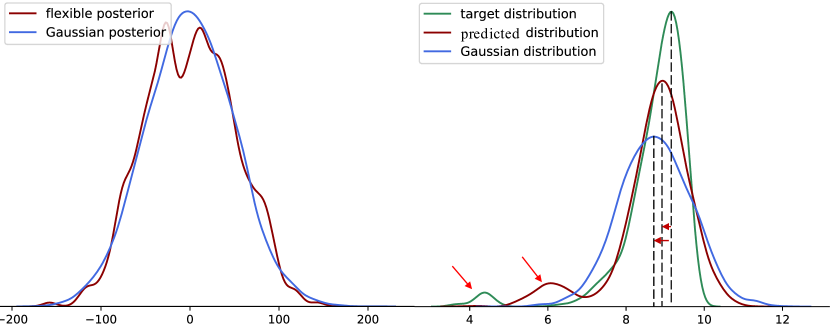
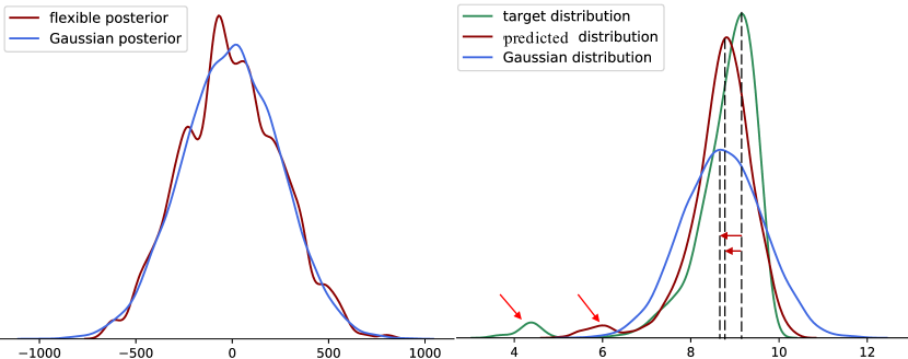
Traffic Forecasting To study the validity of our proposed FDA insightfully, we select three time windows 8:00-10:00 A.M. (the 96$th$ window), 3:00-5:00 P.M. (the 192$nd$ window) and 10:00-12:00 P.M. (the 288$th$ window) at a 7-hour interval. We fit the flexible posterior of FDA and a Gaussian posterior in the left part of Fig. 4. The target distribution, predicted distribution, and Gaussian distribution are compared in the right part. We can see that more details are reserved by the flexible posterior. A specific distribution such as univariate Gaussian cannot approximate target distribution (e.g. multivariate distribution) accurately (red arrows in Fig. 4). The visualization is consistent with the study [57]: the distribution of time series data that changes over time can be better approximated by a dynamic mixture distribution. Although there is a mean left shift (brown arrows in Fig. 4) between target distribution and predicted distribution, the deviation is reduced via learning a flexible distributional representation adaptive to temporal factors.

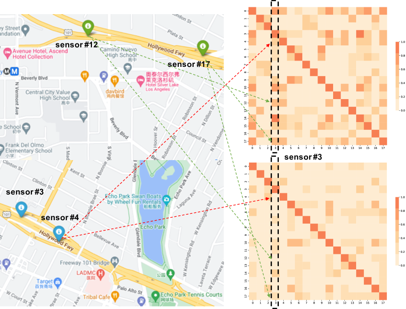
In addition, we choose four sensors from METR-LA and show their corresponding locations on Google Map (left part in Fig. 5). The correlation matrix of different sensors is computed by $\bm{{\rm Z}}^{*}$ on two-time windows 8:00-10:00 A.M. and 10:00-12:00 P.M. (the right part in Fig. 5). The $i$th column in the matrix denotes the correlation strength between sensor $\#i$ and other sensors in the real-world environment. We can observe that the correlation between sensor $\#$3 and sensor $\#$4 is high and hardly varies, while the low correlation between sensor $\#$3 and sensor $\#$12, $\#$17 varies dramatically over time. The results suggest that some sensors are always closely related to each other because of the fixed spatial relationship, however, other sensors are closely related in one-time slice but ‘leave apart’ relations in other time slices. This dynamics is reasonable, since sensor $\#$3 and sensor $\#$12, $\#$17 are located on different main roads surrounded by different environments (schools, parks, etc.). Therefore, the module FDA can capture both invariance and dynamics of time series in the process of distributional drift adaption.

(a) At 8:00-10:00 A.M. (the 96$th$ window)

(b) At 3:00-5:00 P.M. (the 192$nd$ window)

(c) At 10:00-12:00 P.M. (the 288$th$ window)

Figure 4: Distribution of different time windows, METR-LA. The left part is a comparison of flexible and Gaussian posterior in FDA. Comparisons of the target distribution, predicted distribution, and Gaussian distribution are shown in the right part.

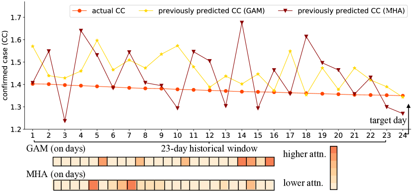
COVID-19 Next, we qualitatively analyze the time-guided component of TCVAE by comparing GAM and traditional multi-head attention (MHA) over a 23-day lookback for the number of confirmed cases (CC) in Zhejiang province in China from the COVID-19 test set in August 2021. We visualize day-level attention throughout the historical window and analyze the corresponding predicted CC for the 24$th$ day in Fig. 6. For comparison, we also show actual and previously predicted CC across all days. TCVAE using MHA predicts the 24$th$ day CC with a relative error of 5.9$\%$ from the actual value, whereas TCVAE using GAM predicts that closer to the actual value (0.44$\%$). Despite the varying trends throughout the historical window, GAM focuses on the gentle descent trend (e.g., the 21$st$ day, the 23$rd$ day) towards the end of the window, whereas MHA learns weighted scores and captures a sharp descent trend (e.g., the 5$th$ day, the 9$th$ day). The results of GAM are consistent with the theory [53]: the impact of long-distance events gradually decays.

Figure 5: Visualization of correlation matrix at 8:00-10:00 A.M. (the 96$th$ window) and 10:00-12:00 P.M. (the 288$th$ window) on 9/1/2018, METR-LA.

Figure 6: Day-level attention visualization and prediction using TCVAE with GAM and MHA methods on COVID-19.

VI Conclusion and Future Work

In this work, a novel variational autoencoder architecture TCVAE for distributional drift adaptation is introduced to model the dynamic dependencies between historical observations and future data varying with time in MTS. Specifically, we design a temporal Hawkes attention mechanism to represent temporal factors that estimate the temporal Gaussian and a gated attention mechanism to dynamically adapt the network structure of the Transformer-based encoder and decoder. We propose to take the advantage of transforming the temporal Gaussian into a flexible distribution that breaks the limitations of distributional form for inferring the temporal conditional distribution. In a variety of MTS forecasting applications, TCVAE based on more robust representation regularly outperforms previous techniques.

We will consider future work from two perspectives. First, TCVAE learns the distributional drift adaptation in estimating the conditional distribution of future data based on the assumption that the distributional drift frequencies of the training and testing sets are the same. The cases of different distribution frequencies often exist in some scenarios. We will consider the dynamics to improve our model in the future. Second, we will explore its application in other real distribution-drift scenarios, such as research hot spots, stock trend forecasting, and product demand analysis.

Hui He received the M.E. degree from University of Shanghai for Science and Technology, Shanghai, China in 2020. She is currently pursuing a Ph.D. degree at the Institute of Engineering Medicine, Beijing Institute of Technology, Beijing, China. Her current research interests focus on multivariate time series analysis and knowledge services.

Qi Zhang received his Ph.D. degree from Beijing Institute of Technology China under the dual Ph.D. program of Beijing Institute of Technology and University of Technology Sydney Australia. He is currently an AI Scientist at DeepBlue Academy of Sciences. His current research interests focus on Collaborative Filtering, learning to hash and sequential recommendation, and multivariate time series analysis.

Kun Yi is a Ph.D. candidate from the Beijing Institute of Technology, China. His current research interests include multivariate time series forecasting, data science, and knowledge discovery.

Kaize Shi (S’20) is with the Institute of Software Intelligence and Software Engineering, Beijing Institute of Technology, and the Australian Artificial Intelligence Institute (AAII), University of Technology Sydney. His current research interests include opinion mining in social networks, social sensor-based emergency management, meteorological knowledge service, knowledge engineering, intelligent transportation, decision support systems.

Zhendong Niu received a Ph.D. degree in computer science from the Beijing Institute of Technology in 1995. He was a Post-Doctoral Researcher with the University of Pittsburgh from 1996 to 1998, a Researcher $\&$ Adjunct from 1999 to 2004, and a Joint Research Professor with Information School, the University of Pittsburgh since 2006. He served as the deputy dean for the School of Software from 2002 to 2006, the deputy dean for the School of Computer Science and Technology from 2006 to 2019, and the director of the Library, Beijing Institute of Technology. His research interests include information retrieval, software architecture, digital libraries, and web-based learning techniques. Prof.Niu is a recipient of the IBM Faculty Innovation Award in 2005 and the New Century Excellent Talents at the University of the Ministry of Education of China in 2006.

Longbing Cao (@SM in 2006) received a Ph.D. in pattern recognition and intelligent systems from the Chinese Academy of Science, China, and a Ph.D. in computing sciences from the University of Technology Sydney, Australia. He is a professor at UTS, an ARC Future Fellow (professorial level), and the EiCs of IEEE Intelligent Systems and J. Data Science and Analytics. His research interests include artificial intelligence, data science, machine learning, behavior informatics, and their enterprise applications.

References

- [1] L. Bai, L. Yao, C. Li, X. Wang, and C. Wang, “Adaptive graph convolutional recurrent network for traffic forecasting,” in Proc. NeurIPS, 2020.
- [2] R. Cirstea, B. Yang, C. Guo, T. Kieu, and S. Pan, “Towards spatio-temporal aware traffic time series forecasting-full version,” CoRR, vol. abs/2203.15737, 2022.
- [3] L. Zhang, C. C. Aggarwal, and G. Qi, “Stock price prediction via discovering multi-frequency trading patterns,” in Proc. KDD, 2017, pp. 2141–2149.
- [4] S. W. Lee and H. Y. Kim, “Stock market forecasting with super-high dimensional time-series data using convlstm, trend sampling, and specialized data augmentation,” Expert Syst. Appl., vol. 161, p. 113704, 2020.
- [5] D. T. Tran, A. Iosifidis, J. Kanniainen, and M. Gabbouj, “Temporal attention-augmented bilinear network for financial time-series data analysis,” IEEE Trans. Neural Networks Learn. Syst., vol. 30, no. 5, pp. 1407–1418, 2019.
- [6] D. Xu, W. Cheng, B. Zong, D. Song, J. Ni, W. Yu, Y. Liu, H. Chen, and X. Zhang, “Tensorized LSTM with adaptive shared memory for learning trends in multivariate time series,” in Proc. AAAI, 2020, pp. 1395–1402.
- [7] G. Spadon, S. Hong, B. Brandoli, S. Matwin, J. F. R. Jr., and J. Sun, “Pay attention to evolution: Time series forecasting with deep graph-evolution learning,” IEEE Trans. Pattern Anal. Mach. Intell., vol. 44, no. 9, pp. 5368–5384, 2022.
- [8] D. Cao, Y. Wang, J. Duan, C. Zhang, X. Zhu, C. Huang, Y. Tong, B. Xu, J. Bai, J. Tong, and Q. Zhang, “Spectral temporal graph neural network for multivariate time-series forecasting,” in Proc. NeurIPS, 2020.
- [9] L. Cao, Q. Liu, and W. Hou, “COVID-19 modeling: A review,” CoRR, vol. abs/2104.12556, 2021.
- [10] M. W. Watson, “Vector autoregressions and cointegration,” Working Paper Series, Macroeconomic Issues, vol. 4, 1993.
- [11] M. W. Seeger, D. Salinas, and V. Flunkert, “Bayesian intermittent demand forecasting for large inventories,” in Proc. NIPS, 2016, pp. 4646–4654.
- [12] X. Chen and L. Sun, “Bayesian temporal factorization for multidimensional time series prediction,” IEEE Trans. Pattern Anal. Mach. Intell., pp. 1–1, 2021.
- [13] G. Lai, W. Chang, Y. Yang, and H. Liu, “Modeling long- and short-term temporal patterns with deep neural networks,” in Proc. SIGIR, 2018, pp. 95–104.
- [14] S. Shih, F. Sun, and H. Lee, “Temporal pattern attention for multivariate time series forecasting,” Mach. Learn., vol. 108, no. 8-9, pp. 1421–1441, 2019.
- [15] K. Bandara, C. Bergmeir, and H. Hewamalage, “Lstm-msnet: Leveraging forecasts on sets of related time series with multiple seasonal patterns,” IEEE Trans. Neural Networks Learn. Syst., vol. 32, no. 4, pp. 1586–1599, 2021.
- [16] W. Zheng and J. Hu, “Multivariate time series prediction based on temporal change information learning method,” IEEE Trans. Neural Networks Learn. Syst., pp. 1–15, 2022.
- [17] R. Sen, H. Yu, and I. S. Dhillon, “Think globally, act locally: A deep neural network approach to high-dimensional time series forecasting,” in Proc. NeurIPS, 2019, pp. 4838–4847.
- [18] H. Zhou, S. Zhang, J. Peng, S. Zhang, J. Li, H. Xiong, and W. Zhang, “Informer: Beyond efficient transformer for long sequence time-series forecasting,” in Proc. AAAI, 2021, pp. 11 106–11 115.
- [19] S. Liu, H. Yu, C. Liao, J. Li, W. Lin, A. X. Liu, and S. Dustdar, “Pyraformer: Low-complexity pyramidal attention for long-range time series modeling and forecasting,” in Proc. ICLR, 2022.
- [20] L. Cao, “Non-iidness learning in behavioral and social data,” Comput. J., vol. 57, no. 9, pp. 1358–1370, 2014.
- [21] W. Li, X. Yang, W. Liu, Y. Xia, and J. Bian, “DDG-DA: data distribution generation for predictable concept drift adaptation,” in Proc. AAAI, 2022, pp. 4092–4100.
- [22] Y. Zhou, C. Liang, N. Li, C. Yang, S. Zhu, and R. Jin, “Robust online matching with user arrival distribution drift,” in Proc. AAAI, 2019, pp. 459–466.
- [23] C. Liu, Y. Li, X. Zhao, C. Peng, Z. Lin, and J. Shao, “Concept drift adaptation for CTR prediction in online advertising systems,” CoRR, vol. abs/2204.05101, 2022.
- [24] J. Kirkpatrick, R. Pascanu, N. Rabinowitz, and et al., “Overcoming catastrophic forgetting in neural networks,” Proceedings of the National Academy of Sciences, vol. 114, no. 13, pp. 3521–3526, 2017.
- [25] Z. Yue, Y. Wang, J. Duan, T. Yang, C. Huang, and B. Xu, “Learning timestamp-level representations for time series with hierarchical contrastive loss,” CoRR, vol. abs/2106.10466, 2021.
- [26] X. You, M. Zhang, D. Ding, F. Feng, and Y. Huang, “Learning to learn the future: Modeling concept drifts in time series prediction,” in Proc. CIKM, 2021, pp. 2434–2443.
- [27] T. Zhao, R. Zhao, and M. Eskénazi, “Learning discourse-level diversity for neural dialog models using conditional variational autoencoders,” in Proc. ACL (1), 2017, pp. 654–664.
- [28] X. Gu, K. Cho, J. Ha, and S. Kim, “Dialogwae: Multimodal response generation with conditional wasserstein auto-encoder,” in Proc. ICLR (Poster), 2019.
- [29] H. Yang, X. Yao, Y. Duan, J. Shen, J. Zhong, and K. Zhang, “Progressive open-domain response generation with multiple controllable attributes,” in Proc. IJCAI, 2021, pp. 3279–3285.
- [30] R. Jankovic, I. Mihajlovic, and A. Amelio, “Time series vector autoregression prediction of the ecological footprint based on energy parameters,” CoRR, vol. abs/1910.11800, 2019.
- [31] D. Salinas, M. Bohlke-Schneider, L. Callot, R. Medico, and J. Gasthaus, “High-dimensional multivariate forecasting with low-rank gaussian copula processes,” in Proc. NeurIPS, 2019, pp. 6824–6834.
- [32] Q. Wang, S. Ren, Y. Xia, and L. Cao, “BiCMTS: Bidirectional coupled multivariate learning of irregular time series with missing values,” in Proc. CIKM, 2021, pp. 3493–3497.
- [33] F. Ilhan, O. Karaahmetoglu, I. Balaban, and S. S. Kozat, “Markovian rnn: An adaptive time series prediction network with hmm-based switching for nonstationary environments,” IEEE Trans. Neural Networks Learn. Syst., pp. 1–14, 2021.
- [34] S. Huang, D. Wang, X. Wu, and A. Tang, “Dsanet: Dual self-attention network for multivariate time series forecasting,” in Proc. CIKM, 2019, pp. 2129–2132.
- [35] N. Mohajerin and S. L. Waslander, “Multistep prediction of dynamic systems with recurrent neural networks,” IEEE Trans. Neural Networks Learn. Syst., vol. 30, no. 11, pp. 3370–3383, 2019.
- [36] Z. Wu, S. Pan, G. Long, J. Jiang, and C. Zhang, “Graph wavenet for deep spatial-temporal graph modeling,” in Proc. IJCAI, 2019, pp. 1907–1913.
- [37] B. Yu, H. Yin, and Z. Zhu, “Spatio-temporal graph convolutional networks: A deep learning framework for traffic forecasting,” in Proc. IJCAI, 2018, pp. 3634–3640.
- [38] Z. Wu, S. Pan, G. Long, J. Jiang, X. Chang, and C. Zhang, “Connecting the dots: Multivariate time series forecasting with graph neural networks,” in Proc. KDD, 2020, pp. 753–763.
- [39] H. He, Q. Zhang, S. Bai, K. Yi, and Z. Niu, “CATN: cross attentive tree-aware network for multivariate time series forecasting,” in Proc. AAAI, 2022, pp. 4030–4038.
- [40] Y. Lyu, M. Li, X. Huang, U. Guler, P. Schaumont, and Z. Zhang, “Treernn: Topology-preserving deep graph embedding and learning,” in Proc. ICPR, 2020, pp. 7493–7499.
- [41] N. Nguyen and B. Quanz, “Temporal latent auto-encoder: A method for probabilistic multivariate time series forecasting,” in Proc. AAAI, 2021, pp. 9117–9125.
- [42] V. Fortuin, M. Hüser, F. Locatello, H. Strathmann, and G. Rätsch, “SOM-VAE: interpretable discrete representation learning on time series,” in Proc. ICLR (Poster), 2019.
- [43] A. Desai, C. Freeman, Z. Wang, and I. Beaver, “Timevae: A variational auto-encoder for multivariate time series generation,” CoRR, vol. abs/2111.08095, 2021.
- [44] J. Kim, J. Kong, and J. Son, “Conditional variational autoencoder with adversarial learning for end-to-end text-to-speech,” in Proc. ICML, vol. 139, 2021, pp. 5530–5540.
- [45] B. Askari, J. Szlichta, and A. Salehi-Abari, “Variational autoencoders for top-k recommendation with implicit feedback,” in Proc. SIGIR, 2021, pp. 2061–2065.
- [46] M. Prakash, A. Krull, and F. Jug, “Fully unsupervised diversity denoising with convolutional variational autoencoders,” in Proc. ICLR, 2021.
- [47] T. Ma, J. Chen, and C. Xiao, “Constrained generation of semantically valid graphs via regularizing variational autoencoders,” in Proc. NeurIPS, 2018, pp. 7113–7124.
- [48] R. Abdal, P. Zhu, N. J. Mitra, and P. Wonka, “Styleflow: Attribute-conditioned exploration of stylegan-generated images using conditional continuous normalizing flows,” ACM Trans. Graph., vol. 40, no. 3, pp. 21:1–21:21, 2021.
- [49] M. Kumar, M. Babaeizadeh, D. Erhan, C. Finn, S. Levine, L. Dinh, and D. Kingma, “Videoflow: A conditional flow-based model for stochastic video generation,” in Proc. ICLR, 2020.
- [50] Y. Luo, K. Yan, and S. Ji, “Graphdf: A discrete flow model for molecular graph generation,” in Proc. ICML, vol. 139, 2021, pp. 7192–7203.
- [51] Z. Zhang, C. Yu, S. Xu, and H. Li, “Learning flexibly distributional representation for low-quality 3d face recognition,” in Proc. AAAI, 2021, pp. 3465–3473.
- [52] K. Rasul, A. Sheikh, I. Schuster, U. M. Bergmann, and R. Vollgraf, “Multivariate probabilistic time series forecasting via conditioned normalizing flows,” in Proc. ICLR, 2021.
- [53] R. Sawhney, S. Agarwal, A. Wadhwa, T. Derr, and R. R. Shah, “Stock selection via spatiotemporal hypergraph attention network: A learning to rank approach,” in Proc. AAAI, 2021, pp. 497–504.
- [54] T. M. Lai, Q. H. Tran, T. Bui, and D. Kihara, “A gated self-attention memory network for answer selection,” in Proc. EMNLP/IJCNLP (1), 2019, pp. 5952–5958.
- [55] H. Ding and X. Luo, “Attentionrank: Unsupervised keyphrase extraction using self and cross attentions,” in Proc. EMNLP (1), 2021, pp. 1919–1928.
- [56] J. Deng, X. Chen, R. Jiang, X. Song, and I. W. Tsang, “St-norm: Spatial and temporal normalization for multi-variate time series forecasting,” in Proc. KDD, 2021, pp. 269–278.
- [57] Y. Wu, J. Ni, W. Cheng, B. Zong, D. Song, Z. Chen, Y. Liu, X. Zhang, H. Chen, and S. B. Davidson, “Dynamic gaussian mixture based deep generative model for robust forecasting on sparse multivariate time series,” in Proc. AAAI, 2021, pp. 651–659.
![[Uncaptioned image]](/html/2209.00654/assets/x16.png) |