Analytic Smoothing and Nekhoroshev estimates for Hölder steep Hamiltonians

Abstract.

In this paper we prove the first result of Nekhoroshev stability for steep Hamiltonians in Hölder class. Our new approach combines the classical theory of normal forms in analytic category with an improved smoothing procedure to approximate an Hölder Hamiltonian with an analytic one. It is only for the sake of clarity that we consider the (difficult) case of Hölder perturbations of an analytic integrable Hamiltonian, but our method is flexible enough to work in many other functional classes, including the Gevrey one. The stability exponents can be taken to be $(\ell-1)/(2n{\bm{\alpha}}_{1}...{\bm{\alpha}}_{n-2})+1/2$ for the time of stability and $1/(2n{\bm{\alpha}}_{1}...{\bm{\alpha}}_{n-1})$ for the radius of stability, $n$ being the dimension, $\ell>n+1$ being the regularity and the ${\bm{{\alpha}}}_{i}$’s being the indices of steepness. Crucial to obtain the exponents above is a new non-standard estimate on the Fourier norm of the smoothed function. As a byproduct we improve the stability exponents in the $C^{k}$ class, with integer $k$.

1. Introduction and main results

1.  The main goal of this work is to introduce a unified way for proving “long time stability” of the action variables for perturbations of completely integrable Hamiltonian systems which belong to a large class of function spaces. We will limit ourselves here to Hölder perturbations of analytic systems, but our method is flexible enough to be adapted to many other settings.

The effective stability theory for nearly-integrable hamiltonian systems was initiated by the pioneering work of J.E. Littlewood [14] and reached a first main achievement in the seventies with the work of N.N. Nekhoroshev [19]; it was then developed by many authors. The usual setting is that of Hamiltonian systems of the form

(1.1) $$H(I,\theta)=h(I)+f(I,\theta),$$

where $(I,\theta)\in\mathbb{R}^{n}\times\mathbb{T}^{n}$ are the action-angle variables and $f$ is small with respect to $h$. In Nekhoroshev’s work the Hamiltonian $H$ is analytic and $h$ satisfies a steepness condition (see definition 1.1 below). The theory has been then developed in various settings: $H$ can be assumed to be Gevrey (which includes the analytic case) or $C^{k}$ with $k\geq 2$ and integer, while $h$ can be assumed to be convex or quasi-convex (see for example [18] or [5])

The norm of $f$, relative to the function space at hand, is denoted by $\varepsilon$. For systems as (1.1), the previous results assert that the action variables are confined in a ball of radius ${\bf R}(\varepsilon)$ centered at the initial action during a time ${\bf T}(\varepsilon)$, provided that $\varepsilon$ is smaller that some threshold ${\bf E}$. We say that ${\bf R}(\varepsilon)$ is the confinement radius, ${\bf T}(\varepsilon)$ is the stability time and ${\bf E}$ is the applicability threshold. The remarkable fact is that – $h$ being given – the results depend only on the norm of $f$ and not on its particular form.

Much attention has been paid in the literature in order to obtain good estimates for the quantities ${\bf R}(\varepsilon)$ and ${\bf T}(\varepsilon)$ in the different frameworks. As we shall see in the sequel, in the setting of Hölder perturbations of analytic integrable systems, the method we introduce in this paper yields sharper estimates than those that are found in the literature up to now. Before stating rigorously our results, however, it is useful to have an overview of the classical results on the effective stability of near-integrable Hamiltonian systems.

2.  The classical results. Let us briefly describe the classical abstract results. In the 70’s Nekhoroshev proved his seminal theorem [19], which asserts that for a steep real-analytic function $h$ and for any real-analytic perturbation $f$ with analytic extension to a complex domain ${\mathcal{D}}$, all solutions are stable at least over exponentially long time intervals. Namely, there exist positive exponents $a$, $b$ and a positive threshold ${\bf E}$, depending only on $h$, such that if ${\left|f\right|}_{{\mathcal{D}}}\leq{\bf E}$, then any initial condition $(I_{0},\theta_{0})$ gives rise to a solution $\big{(}I(t),\theta(t)\big{)}$ which is defined at least for ${\left|t\right|}\leq\exp\big{(}c(1/\varepsilon)^{a}\big{)}$ and satisfies ${\left|I(t)-I_{0}\right|}\leq C\varepsilon^{b}$ in that range. Here ${\left|f\right|}_{{\mathcal{D}}}$ is the $C^{0}$ sup-norm on the domain ${\mathcal{D}}$ and $c$, $C$ are positive constants which also depend only on $h$. With our notation, for these systems:

(1.2) $${\bf T}(\varepsilon)=\exp(c(1/\varepsilon)^{a}),\qquad{\bf R}(\varepsilon)=C\varepsilon^{b},$$

while the expression of the threshold ${\bf E}$ is quite difficult to obtain explicitly, see [19]. Since the constants $c$ and $C$ are less significant than the exponents we will get rid of them in our subsequent description.

Nekhoroshev’s proof is based on the construction of a partition (a “patchwork”) of the phase space into zones of approximate resonances of different multiplicities, over which one can construct adapted normal forms. The global stability result necessitates a very delicate control of the size and disposition of the elements of the patchwork in order to produce a “dynamical confinement” preventing the orbits from fast motions along distances larger than the confinement radius (see below for a discussion).

In the convex case, as noticed in [11] and [4], a shrewd use of energy conservation leads to a much simpler and “physical” way to confine the orbits. This gave rise to two distinct series of works, originating in the articles of Lochak [15] - where the simultaneous approximation method was introduced - and Pöschel [23] - where the construction of Nekhoroshev’s patchwork was made much easier - both relying on the convexity or quasi-convexity of the integrable Hamiltonian.

The simplicity of these methods made it possible to prove that the Nekhoroshev Theorem in the analytic case holds with

(1.3) $${\bf T}(\varepsilon)=\exp(c(1/\varepsilon)^{1/2n}),\qquad{\bf R}(\varepsilon)=C\varepsilon^{1/2n},$$

if $h$ is assumed to be quasi-convex (see [15, 17, 23]). Moreover, besides the global result, one can state local results for neighborhoods of resonant surfaces. For $m\in\{1,\ldots,n-1\}$, consider a sublattice $\Lambda\in\mathbb{Z}^{n}_{K}:=\{k\in\mathbb{Z}^{n}:|k|_{1}\leq K\}$ of rank $m$ and the resonant subset ${\mathcal{M}}_{\Lambda}:=\{I\in\mathbb{R}^{n}\mid\nabla h(I)\in\Lambda^{\bot}\}$. Then, for all trajectories starting at a distance of order $\varepsilon^{1/2}$ of ${\mathcal{M}}_{\Lambda}$, one gets larger stability exponents, namely $a=b=1/(2(n-m))$. Moreover, in the resonant block ${\mathcal{B}}_{\Lambda}$ (which is obtained by eliminating from ${\mathcal{M}}_{\Lambda}$ all the intersections with other resonant subsets ${\mathcal{M}}_{\Lambda^{\prime}}$, with $\text{rank }\Lambda^{\prime}=m+1$) one can even take $a=1/(2(n-m)),\ b=1/2$.

As alluded to above, long time stability does not require a priori the analyticity of the Hamiltonian at hand. For general Gevrey quasi-convex systems, the fast decay of the Fourier coefficients also yields exponentially long stability times. Namely, for $\beta$-Gevrey systems (where $\beta$ is the Gevrey exponent) it is proved in [18] that

$${\bf T}(\varepsilon)=\exp\big{(}c/\varepsilon^{1/(2n\beta)}\big{)},\qquad{\bf R}(\varepsilon)=C\varepsilon^{1/(2n\beta)}.$$

The proof is based on a direct construction of normal forms for Gevrey systems. This study was initiated by M. Herman for proving the optimality of the stability exponents by constructing explicit examples taking advantage of the flexibility of the Gevrey category, see below.

Soon after, finitely differentiable systems have been investigated in [5] using a direct implementation of Lochak’s scheme in this setting, which yields the estimates

$${\bf T}(\varepsilon)=c/\varepsilon^{(\ell-2)/(2n)}\qquad{\bf R}(\varepsilon)=C\varepsilon^{1/(2n)}$$

for quasi-convex $C^{\ell}$ systems with $\ell\geq 2$ and integer. On the other hand, the stability of $C^{\ell}$ systems, with $\ell$ an integer such that $\ell\geq\ell^{*}n+1$ for some suitable $\ell^{*}\geq 1,\ell^{*}\in{\mathbb{N}}$, satisfying a property known as Diophantine-Morse condition, was investigated in [6], where the values

$${\bf T}(\varepsilon)=c/\varepsilon^{\ell^{*}/[3(4(n+1))^{n}]}\qquad{\bf R}(\varepsilon)=C\varepsilon^{1/(4(n+1))^{n}}$$

were found.

The case $\ell=+\infty$ has been studied in [1], where the authors find that, in the case $h(I)=I^{2}/2$ and for fixed $b\in(0,1/2)$, for any $M>0$ there exists $C_{M}>0$ such that

$${\bf T}(\varepsilon)=\frac{C_{M}}{\varepsilon^{M}}\qquad{\bf R}(\varepsilon)=C_{M}\varepsilon^{b}\ .$$

The result is achieved by implementing an innovative global normal form in Pöschel’s framework.

Finally, we also refer to the recent work [7] and references therein for much more information about stability in various functional classes.

3.  Purpose of the work. The objective of this paper is to make a systematic use of analytic smoothing methods to derive normal forms in a very simple way - whatever the regularity of the Hamiltonians at hand - from the usual analytic ones. This way we get maximal flexibility to adapt the different long-time stability proofs to a large class of function spaces. We will investigate here only the case of Hölder differentiable Hamiltonians, but our method extends to any steep functions belonging to any regularity class which admits an analytic smoothing. More precisely, the proposed strategy (see Section 4.3) allows us to prove, in a very simple way, the first Nekoroshev-type result of stability for Hölder steep Hamiltonians with presumed sharp exponents. In this case one cannot expect to get more than polynomial stability times relative to the size $\varepsilon$ of the perturbation [5]. In the course of the proof we need to adjust in a rather unusual way the size of the various parameters: ultraviolet cutoff and, in an essential way, the analyticity width, as a function of the size $\varepsilon$ of the perturbation.

4.  Main results. Let us fix the main definitions and assumptions. In the following, given $\nu\in{\left\{1,\ldots,\infty\right\}}$, we denote by $|\cdot|_{\nu}$ the corresponding $\ell^{\nu}$-norm in $\mathbb{R}^{n}$ or $\mathbb{C}^{n}$. We denote by $B_{\nu}(I_{0},R)$ the open ball centered at $I_{0}$ of radius $R$ for the norm ${\left|\,\cdot\,\right|}_{\nu}$ in $\mathbb{R}^{n}$.

Consider a Hamiltonian of the form (1.1), where we assume, for the sake of simplicity, that the unperturbed part $h$ is analytic while only the perturbation $f$ is Hölder, so:

(1.4) $$h\in C^{\omega}(B_{\infty}(0,R)_{\rho_{0}}),\qquad f\in C^{\ell}(B_{\infty}(0,R)\times\mathbb{T}^{n}),$$

where $B_{\infty}(0,R)_{\rho_{0}}$ is the complex extension of analyticity width $\rho_{0}\geq 1$ of $B_{\infty}(0,R)$, and $\ell\in(1,+\infty)$ (meaning that $f$ is Hölder differentiable when $\ell$ is not an integer, see section 3 for a brief overview on this class of functions). The small parameter is

(1.5) $$\varepsilon:=|f|_{C^{\ell}(B_{\infty}(0,R)\times\mathbb{T}^{n})},$$

(see (3.2) for a definition of the Hölder norm). We denote by ${\omega}=\nabla h:\mathbb{R}^{n}\to\mathbb{R}^{n}$ the action-to-frequency map attached to $h$.

We will assume that the Hessian of $h$ is uniformly bounded from above:

(1.6) $$M:=\sup_{I\in B_{\infty}(0,R)_{\rho_{0}}}\left\lVert D^{2}h(I)\right\rVert_{op}<\infty,$$

where $\left\lVert\ \right\rVert_{op}$ stands for the operator norm induced by the Hermitian norm on $\mathbb{C}^{n}$.

We will also assume that the Hamiltonian $h$ is steep according to the following definition.

Definition 1.1 (Steepness).

Fix $\delta>0$. A $C^{1}$ function $h:B_{\infty}(0,R+\delta)\to\mathbb{R}$ is steep with steepness indices ${\bm{\alpha}}_{1},\ldots,{\bm{\alpha}}_{n-1}\geq 1$ and steepness coefficients $C_{1},\ldots,C_{n-1},\delta$ if:

1. $\inf_{B_{\infty}(0,R)}{\left|{\omega}(I)\right|}_{2}>0$;

2. for any $I\in B_{\infty}(0,R)$ and any $m$-dimensional subspace $\Gamma$ orthogonal to ${\omega}(I)$, with $1\leq m<n$:

   (1.7) $$\max_{0\leq\eta\leq\xi}\,\min_{u\in\Gamma,{\left|u\right|}_{2}=\eta}{\left|\pi_{\Gamma}{\omega}(I+u)\right|}_{2}>C_{m}\xi^{{\bm{\alpha}}_{m}},\quad\forall\xi\in(0,\delta],$$

   where $\pi_{\Gamma}$ stands for the orthogonal projection on $\Gamma$.

Remark 1.1.

Note that a uniformly strictly convex function is steep with steepness indices equal to $1$.

Remark 1.2.

The steepness condition is generic in the space of jets of sufficiently regular functions (see [20] for the general discussion and [25], [2] for sufficient conditions for steepness in the space of jets of order four and five respectively).

Our main theorem is the following.

Theorem 1.1 (Stability estimates in the steep case).

Consider a near-integrable Hamiltonian system (1.1) satisfying (1.4) and assume $\ell\geq n+1$ . Suppose that $h$ is steep in $B_{\infty}(0,R)$ with steepness indices ${\bm{\alpha}}:=({\bm{\alpha}}_{1},\ldots,{\bm{\alpha}}_{n-1})$ and set:

$$\mathtt{a}:=\frac{\ell-1}{2n{\bm{\alpha}}_{1}\times\cdots\times{\bm{\alpha}}_{n-2}}+\frac{1}{2}\quad,\qquad\mathtt{b}:=\frac{1}{2n{\bm{\alpha}}_{1}\times\cdots\times{\bm{\alpha}}_{n-1}}\ .$$

Then, there exist positive constants ${\bf E}={\bf E}(n,\ell,{\bm{\alpha}}),{\mathtt{C}}^{\prime\prime}_{\bf I}:={\mathtt{C}}^{\prime\prime}_{\bf I}(n,\ell,{\bm{\alpha}})$, ${\mathtt{C}}^{\prime\prime}_{\bf T}:={\mathtt{C}}^{\prime\prime}_{\bf T}(n,\ell,{\bm{\alpha}})$ such that, for $\varepsilon\leq{\bf E}$, the radius and time of confinement relative to any initial condition in the set $B_{\infty}(0,R/4)$ satisfy:

(1.8) $${\bf R}(\varepsilon)\leq{\mathtt{C}}^{\prime\prime}_{{\bf I}}\varepsilon^{\mathtt{b}}\quad,\qquad{\bf T}(\varepsilon)\leq{\mathtt{C}}^{\prime\prime}_{{\bf T}}\frac{1}{|\ln\varepsilon|^{\ell-1}\,\varepsilon^{\mathtt{a}}}\,.$$

Remark 1.3.

$\bullet$ The presence of the logarithm in (1.8) comes from the fact that in our method we have some freedom to fix the analyticity width depending on $\varepsilon$, in contrast with the classical analytic setting. We send the reader to Remark 5.1, where this comment is contextualized, the dependence of the analyticity width in $\varepsilon$ is made precise and a qualitative justification is given.  
$\bullet$ If we set ${\bm{\alpha}}_{1},\ldots,{\bm{\alpha}}_{n-1}=1$ (i.e. the convex case) we obtain better estimates than in [5].  
$\bullet$ Our proof relies on the geometric construction of the geography of resonances introduced in [13], which is appropriate only for Hamiltonians in $n\geq 3$ degrees of freedom. Here too we shall restrict to this setting, the $2$ d.o.f. isoenergetic non-degenerate case being easily managed through KAM theory. A specific construction should be implemented to treat the peculiarity of the isoenergetic degenerate $2$ d.o.f. case. This study is in progress in a forthcoming work.

5.  Prospects.

The sharpness of the exponents in Theorem 1.1 should be proved in the same way as in the case of convex system. The first attempt to tackle this problem led to work in the Gevrey category instead of the analytic one and construct examples with unstable orbits, which experience a drift in action of the same order as the confinement radius within a time of the same order as the stability time, see [18]. It has then be realized that the initial conjecture in quasi-convex analytic systems ($a\sim 1/2n$, see [10] and Lochak [15]) was in fact incorrect: as proved in [8] using a purely topological argument together with the previous remark on the local exponents near simple resonances, one can choose $a=1/(2(n-1))$ as a global stability exponent for ${\bf T}(\varepsilon)$. This result was improved soon after with $a\sim 1/(2(n-2))$ (see [26]). The construction of unstable system proving the optimality of these latter exponents was achieved in [18], [16], [26]. A remarkable fact is that the unstable mechanism introduced by Arnold in the 60’s, with its subsequent improvements, is exactly what is needed to produce the unstable examples in the quasi-convex case.

As for the steep case, a careful construction of the geography of resonances leads with strong evidence to the conjecture that the exponents $a=1/(2n{\bm{\alpha}}_{1}...{\bm{\alpha}}_{n-2})$ and $b=1/(2n{\bm{\alpha}}_{1}...{\bm{\alpha}}_{n-1})$ are sharp (see ref. [13]). The question of constructing explicit examples with unstable orbits proving this sharpness is still open nowadays and is maybe the last challenging problem in the general long time stability theory, probably relying on new Arnold diffusion ideas.

The paper is organized as follows: in the next section we give a short overview of the classical methods with particular attention on the geometry of resonant blocks, on which the present work strongly relies. Next we define the functional setting. In Section 4 we introduce the analytic smoothing appropriately adapted to our problem. Finally Section 5 is devoted to the study of the steep case.

Acknowledgements

We wish to thank A. Bounemoura, L. Biasco, L. Chierchia, M. Salvatori, and L. Niederman for fruitful discussions and stimulating comments, which definitively helped to improve this work. J.E.M. acknowledges the support of the INdAM-GNAMPA grant “Spectral and dynamical properties of Hamiltonian systems”.

2. General setting and classical methods: a geometric framework

1.  Resonances, resonant normal forms and the steepness condition. Consider a Hamiltonian system of the form (1.1) defined on $O\times\mathbb{T}^{n}$, where $O$ is an open subset of $\mathbb{R}^{n}$. The main feature underlying Hamiltonian perturbation theory is that one can modify the form of the perturbation $f$ by composing $H$ with properly chosen local Hamiltonian diffeomorphisms, in order to remove a large number of “nonessential harmonics”. The result of this process - a local normal form - strongly depends on the location of the domain of the normalizing diffeomorphism w.r.t the resonances of the unperturbed part $h$, and enables one to discriminate between fast drift and extremely slow drift directions in the action space, according to this location.

Let us first make this idea more precise. Given an integer lattice $\Lambda\subset\mathbb{R}^{n}$ of dimension $m\in\{1,\ldots,n-1\}$ – a resonance lattice – one associates with $\Lambda$ the resonance vector subspace $\Lambda^{\bot}\subset\mathbb{R}^{n}$ in the frequency space $\mathbb{R}^{n}$, together with the corresponding resonance subset in the action space previously introduced

$${\mathcal{M}}_{\Lambda}:={\omega}^{-1}(\Lambda^{\bot})=\{I\in O\mid{\omega}(I)\in\Lambda^{\bot}\},$$

where ${\omega}=\nabla h$ is the frequency map. The dimension $m$ of $\Lambda$ is said to be the multiplicity of the resonance ${\mathcal{M}}_{\Lambda}$. Of course, given a resonance module $\Lambda^{\prime}\supset\Lambda$ with $\dim\Lambda^{\prime}>\dim\Lambda$, the resonance ${\mathcal{M}}_{\Lambda^{\prime}}$ is contained in ${\mathcal{M}}_{\Lambda}$, so that a resonance subset contains in general infinitely many resonances of higher multiplicity. The complement ${\mathcal{M}}_{0}\subset O$ of the union of all resonance subsets is the non-resonant subset. In general, a resonance subset ${\mathcal{M}}_{\Lambda}$ has no particular structure, however, one can think of ${\mathcal{M}}_{\Lambda}$ as a submanifold of $\mathbb{R}^{n}$ of the same dimension as $\Lambda^{\bot}$ (with perharps singular loci).

As a rule, when $\varepsilon$ is small enough, for a small enough $\varepsilon$-depending neighborhood $W_{\Lambda}$ of the parts of the resonance subset ${\mathcal{M}}_{\Lambda}$ located far enough from resonances of higher multiplicity, one can iteratively construct a symplectic diffeomorphism $\Psi_{\Lambda}$, whose image contains $W_{\Lambda}\times\mathbb{T}^{n}$, such that the pull-back $H_{\Lambda}=H\circ\Psi_{\Lambda}$ takes the following form

(2.1) $$H_{\Lambda}=h+N_{\Lambda}+R_{\Lambda}.$$

Here $R_{\Lambda}$ is a remainder whose $C^{2}$ norm is (very) small with respect to $\varepsilon$ and the resonant part $N_{\Lambda}$ contains only harmonics belonging to $\Lambda$, that is:

$$N_{\Lambda}(I,\theta)=\sum_{k\in\Lambda,\,{\left|k\right|}_{1}\leq K(\varepsilon)}a_{k}(I)\,e^{ik\cdot\theta},$$

where $K(\varepsilon)$ is an ultraviolet cutoff which has to be properly chosen. Both terms $N_{\Lambda}$ and $R_{\Lambda}$ of course depend on $\varepsilon$. A subset $W_{\Lambda}$ for which such a normal form is proved to exist will be called a normal form neighborhood associated with $\Lambda$, with multiplicity $\dim\Lambda$. One proves that the space of actions can be covered by such neighborhoods, and in Section 5.1, we will construct finer covers by subsets of those, named resonant blocks (and denoted by $D_{\Lambda}$ in the aforementioned section).

The iterative process to construct the normalizing diffeomorphism involves the control of small denominators which appear during the resolution of the so-called homological equation, and which depend on the location of the normalization domain with respect to the resonances (see for instance [23]). This can be seen as a drawback of the method which could be greatly simplified by an idea due to Lochak (see below), however the general method presented here give precise dynamical informations which would not be reachable otherwise.

The Hamilton equations generated by (2.1) yield the following form for the evolution of the action variables:

(2.2) $$\begin{array}[]{lll}I(t)-I(0)&=&\displaystyle\int_{0}^{t}\partial_{\theta}N_{\Lambda}\big{(}I(s),\theta(s)\big{)}+\partial_{\theta}R_{\Lambda}\big{(}I(s),\theta(s)\big{)}\,ds\\[8.0pt] &=&\displaystyle\sum_{k\in\Lambda,\,{\left|k\right|}_{1}\leq K(\varepsilon)}k\cdot\Big{(}\int_{0}^{t}i\,a_{k}(I(s))\,e^{ik\cdot\theta(s)}\,ds\Big{)}+{\mathcal{R}}(t).\end{array}$$

The variation of $I$ is therefore the sum of the main part

(2.3) $${\mathcal{D}}(t):=\sum_{k\in\Lambda,\,{\left|k\right|}_{1}\leq K(\varepsilon)}k\cdot{\mathcal{N}}^{(k)}(t),\qquad{\mathcal{N}}^{(k)}(t)=\int_{0}^{t}i\,a_{k}(I(s))\,e^{ik\cdot\theta(s)}\,ds,$$

and the very small remainder term ${\mathcal{R}}(t)$.

To simplify the presentation in the following, we will forget about the angles and consider only the action part of the solutions of our system (which is legitimized by the fact that the angles play no role in the various estimates).

The whole theory relies firstly on the obvious fact that the main drift term ${\mathcal{D}}(t)$ in (2.3) belongs to the vector space $\rm Vect\,\Lambda$ spanned by $\Lambda$ (which is often called “plane” of fast drift), and secondly on the smallness of the remainder term ${\mathcal{R}}$. A solution starting from some initial condition $I(0)\in W_{\Lambda}$ will therefore remain very close to the fast drift space

$$I(0)+\rm Vect\,\Lambda$$

during a very long time – governed by the smallness of ${\mathcal{R}}$ – as long as it is contained inside the neighborhood $W_{\Lambda}$. This makes it necessary to understand first the intersections of the fast drift planes $I+\rm Vect\,\Lambda$ and the neighborhoods $W_{\Lambda}$ to which they are attached.

As an extreme example, let us consider the Hamiltonian

$$h(I)=\frac{1}{2}(I_{1}^{2}-I_{2}^{2})$$

on $\mathbb{A}^{2}$, with (invertible) frequency map ${\omega}(I_{1},I_{2})=(I_{1},-I_{2})$. We focus on the resonance module $\Lambda=\mathbb{Z}(1,-1)$, so that $\Lambda^{\bot}=\mathbb{R}(1,1)$ and $\rm Vect\,\Lambda={\mathcal{M}}_{\Lambda}$. Hence, given an initial action $I(0)\in{\mathcal{M}}_{\Lambda}$, the entire fast drift affine subspace $I(0)+\rm Vect\,\Lambda$ coincides with ${\mathcal{M}}_{\Lambda}$, so that nothing prevents the fast drift to take place during the whole motion provided the perturbation is well-chosen: the resonance ${\mathcal{M}}_{\Lambda}$ is called a superconductivity channel. No long time stability result can be expected in this case: indeed, when $f(I,\theta)=\sin(\theta_{1}-\theta_{2})$, the initial condition $I=0$, $\theta=0$ yields the fast evolution $(I_{1}(t),I_{2}(t))=(-\varepsilon t,\varepsilon t)$ for the action variables .

In constrast with the previous example, for the Hamiltonian

$$H(I,\theta)=\frac{1}{2}{{\left|I\right|}}^{2}_{2}+\varepsilon f(\theta)$$

on $\mathbb{A}^{n}$, for any $\Lambda\subset\mathbb{Z}^{n}_{K}$, the the resonant set ${\mathcal{M}}_{\Lambda}$ coincides with $\Lambda^{\bot}$, so that the affine planes of fast drift are always orthogonal to ${\mathcal{M}}_{\Lambda}$. In this case a fast drift - if it happens - makes the orbits move away from the resonance in a very short time.

These extreme examples illustrate the role of the Nekhoroshev condition: steepness is an intermediate quantitative property, which prevents from the existence of the superconductivity channels by ensuring a certain amount of transversality between the fast drift planes and the corresponding resonances in action. Starting from an action $I=I(0)$ located at some resonance ${\mathcal{M}}_{\Lambda}$, so that its associated frequency ${\omega}(I)$ is orthogonal to $\Gamma:=\rm Vect\,\Lambda$, the condition

(2.4) $$\max_{0\leq\eta\leq\xi}\,\min_{u\in\Gamma,{\left|u\right|}_{2}=\eta}{\left|\pi_{\Gamma}{\omega}(I+u)\right|}_{2}>C_{m}\xi^{{\bm{\alpha}}_{m}},\quad\forall\xi\in(0,\delta],$$

(where $\pi_{\Gamma}$ stands for the orthogonal projection on $\Gamma$) imposes that a drift of length $\xi$ starting from $I$ and occuring along the fast drift plane $I+\Gamma$ makes the projection $\pi_{\Gamma}({\omega})$ change by an amount of $C_{m}\xi^{{\bm{\alpha}}_{m}}$ during the way.

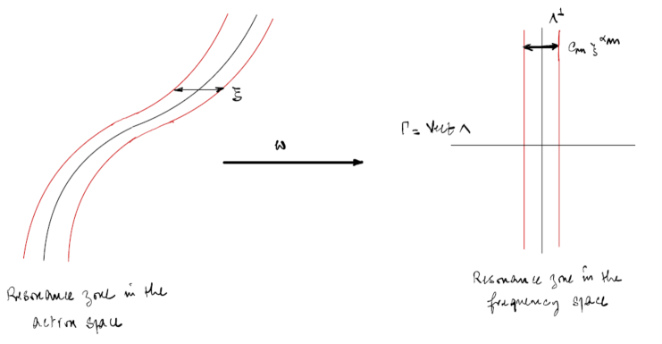
Figure 1. Geometric interpretation of the steep condition

This admits an easy geometric interpretation (see Figure 1). Assume $\dim\Lambda=m$ and consider the vector space $\Gamma$ spanned by $\Lambda$, together with its orthogonal space $\Lambda^{\bot}$ - of dimension $n-m$. Then one can define a family of tubular neighborhoods of $\Lambda^{\bot}$ of width $\delta>0$ by

(2.5) $${\bf T}_{\delta}(\Lambda^{\bot})=\{\varpi\in\mathbb{R}^{n}\mid\pi_{\Gamma}(\varpi)<\delta\},\quad\delta>0\,.$$

Each such neighborhood gives rise to a neighborhood of the resonance ${\mathcal{M}}_{\Lambda}$ in action, namely:

(2.6) $${\bf W}_{\delta}({\mathcal{M}}_{\Lambda})={\omega}^{-1}\big{(}{\bf T}_{\delta}(\Lambda^{\bot})\big{)}.$$

Therefore, condition (2.4) just says that any orbit starting from $I$ and drifting to a distance $\xi$ from $I$ along the plane of fast drift $\Gamma$ must exit the neighborhood ${\bf W}_{\delta}({\mathcal{M}}_{\Lambda})$ with $\delta=C_{m}\xi^{{\bm{\alpha}}_{m}}.$

Note finally that given disjoint subsets ${\bf T}$, ${\bf T}^{\prime}$ of tubular neighborhoods of the form (2.5), the associated neighborhoods ${\omega}^{-1}({\bf T})$ and ${\omega}^{-1}({\bf T}^{\prime})$ are disjoint too, whatever the geometric assumptions on the frequency map ${\omega}$.

2.  Nekhoroshev’s hierarchy. This section is inspired by Nekhoroshev’s ideas as presented in the very nice paper [13]. We also refer to [12] for further details and to [22] for a different approach. Nekhoroshev’s strategy to prove long-time stability results for perturbations of steep Hamiltonians is based on the previous description of resonant neighborhoods, and relies on the following key observation.

Given $\varepsilon$ small enough, there exist $T(\varepsilon)$, $R(\varepsilon)$ and a covering of the action space $O$ by resonant “blocks” $({\mathcal{B}}_{m,p})_{0\leq p\leq p_{m}}$, for ${0\leq m\leq n-1}$, and $m,p,p_{m}\in{\mathbb{N}}$, which satisfy the following properties:

1. $T(\varepsilon)\to+\infty$ and $R(\varepsilon)\to 0$ when $\varepsilon\to 0$;

2. each block ${\mathcal{B}}_{m,p}$ is contained in a resonant neighborhood of multiplicity $m$ and admits an enlargement $\widehat{\mathcal{B}}_{m,p}\supset{\mathcal{B}}_{m,p}$ contained in the same resonant neighborhood;

3. any solution starting from an initial condition in ${\mathcal{B}}_{m,p}$ either stays inside $\widehat{\mathcal{B}}_{m,p}$ for $0\leq t\leq T(\varepsilon)$ or admits a first exit time $t_{1}$ such that $I(t_{1})$ belongs to a block ${\mathcal{B}}_{m^{\prime},p^{\prime}}$ with $m^{\prime}<m$;

4. for any initial condition $I(0)$ inside a block ${\mathcal{B}}_{m,p}$ and for any interval ${\mathcal{I}}$ such that $I(t)\in\widehat{\mathcal{B}}_{m,p}$ for all $t\in{\mathcal{I}}$, then

   $${\left|I(t)-I(0)\right|}_{2}<R(\varepsilon),\quad\forall t\in{\mathcal{I}}.$$

We say that $m$ is the multiplicity of the block ${\mathcal{B}}_{m,p}$. Taking the previous observation for granted, the stability of the action variable over a timescale $T(\varepsilon)$ is easy to prove by finite induction. Given an initial condition $I(0)$ located in some block ${\mathcal{B}}_{m_{0},p_{0}}$, either $I(t)\in\widehat{\mathcal{B}}_{m_{0},p_{0}}$ for $0\leq t\leq T(\varepsilon)$, or there is a $t_{1}$ such that $I(t)\in\widehat{\mathcal{B}}_{m_{0},p_{0}}$ for $0\leq t<t_{1}$ and $I(t_{1})$ belongs to a block ${\mathcal{B}}_{m_{1},p_{1}}$ with $m_{1}<m_{0}$. Consequently, there is a finite sequence $(m_{0},p_{0}),\ldots,(m_{j},p_{j})$ such that $m_{0}>m_{1}>\cdots>m_{j}$ (with maybe $m_{j}=0$) and a finite sequence of times $t_{0}=0<t_{1}<\cdots<t_{p}=T(\varepsilon)$ such that for $0\leq i<j$:

$$I(t)\in\widehat{\mathcal{B}}_{(m_{i},p_{i})},\quad\forall t\in[t_{i},t_{i+1}].$$

In words, any orbits crosses a finite number of enlarged blocks during the interval $[0,T(\varepsilon)]$ and get trapped inside the last one. To conclude, one just has to use property (4), which proves that the distance between $I(0)$ and $I(t)$ is at most $nR(\varepsilon)$ for $t\in[0,T(\varepsilon)]$.

One should be aware that the covering by the blocks is not a partition of $O$: two distinct blocks may have a nonempty intersection. However, one can choose the blocks visited by the orbits according to a hierarchical order, in such a way that their multiplicity decreases as $t$ increases . We say that a covering of $O$ by blocks satisfying the previous properties is a Nekhoroshev patchwork.

3.  Construction of Nekhoroshev patchworks. Let us now describe how the blocks are constructed so as to possess their covering and confinement properties.

Given $\varepsilon>0$, we first fix an ultraviolet cutoff $K(\varepsilon)$ and consider only the set ${\bf M}_{\varepsilon}$ of resonance modules which are spanned by vectors of length smaller than $K(\varepsilon)$. Given a resonant module $\Lambda\in{\bf M}_{\varepsilon}$ of multiplicity $m$, we start with the resonant zone of “width” $\delta_{\Lambda}$

$$Z_{\Lambda}:=W_{\delta_{\Lambda}}({\mathcal{M}}_{\Lambda})={\omega}^{-1}\big{\{}\varpi\in\mathbb{R}^{n}\mid{\left|\pi_{\Gamma}(\varpi)\right|}_{2}<\delta_{\Lambda}\big{\}},$$

where $\delta_{\Lambda}$ has to be properly chosen as a function of $\varepsilon$ and the various geometric invariants of the module (see section 5). We then define the ($\varepsilon$-dependent) resonant zone ${\mathcal{Z}}_{m}$ of multiplicity $m$ as

$$Z_{m}=\bigcup_{\Lambda\in{\bf M}_{\varepsilon},\,\dim\Lambda=m}Z_{\Lambda}.$$

Given $\Lambda\in{\bf M}_{\varepsilon}$, $\dim\Lambda=m$, the block attached to $\Lambda$ is obtained by removing from $Z_{\Lambda}$ its intersection with the complete resonant zone of multiplicity $m+1$:

$${\mathcal{B}}_{\Lambda}=Z_{\Lambda}\setminus Z_{m+1}.$$

The blocks ${\mathcal{B}}_{m,p}$ are the connected components of $Z_{m}$. With no great loss of generality, one can think of (the closure of) a block as a submanifold with boundary and corners – even if it is not necessary.

The following figure shows the construction of the blocks in the case $n=3$ (and in a transverse section). The resonance zone of multiplicity 2 if the disjoint union of the blue blocks, the resonance zone of multiplicity 1 is the union on the strips with red boundaries, while the $0$-multiplicity zone is the complement of the $1$-multiplicity zone.

In any case, the blocks satisfy two main properties.

• The closures of two different blocks can intersect only when their multiplicities are distinct.

This comes from a very careful choice of the widths of the various resonance zones (see [13] and Section 5), which in fact ensures a more stringent (and crucial) property: the enlargement of a block contained in some ${\mathcal{B}}_{\Lambda}$ cannot intersect any other block contained in the zone ${\mathcal{B}}_{\Lambda}$, neither any other neighborhood ${\mathcal{M}}_{\Lambda^{\prime}}$ with $\dim\Lambda^{\prime}=\dim\Lambda$ (see below for precisions on the construction of the enlargement).

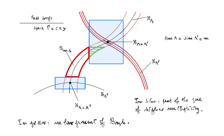
Figure 2. Construction of the resonant blocks

We state the second property in the spirit of Conley’s isolating blocks theory.

• The frontier $\partial{\mathcal{B}}_{m,p}$ of ${\mathcal{B}}_{m,p}$ is the union of two subsets

  $$\partial{\mathcal{B}}_{m,p}=\partial^{+}{\mathcal{B}}_{m,p}+\partial^{-}{\mathcal{B}}_{m,p}$$

  where $\partial^{+}{\mathcal{B}}_{m,p}$ (resp. $\partial^{-}{\mathcal{B}}_{m,p}$) is contained in blocks ${\mathcal{B}}_{m^{\prime},p^{\prime}}$ with $m^{\prime}>m$ (resp. $m^{\prime}<m$).

This raises new questions which could be the starting point of a better understanding of the relations between diffusion along invariant subsets and long-time stability theory. Indeed, given a block ${\mathcal{B}}_{m,p}$, a description of the (generic) features of the Hamiltonian vector field $X_{H_{\varepsilon}}$ at the frontier $\partial{\mathcal{B}}_{m,p}$ has never been done. In particular, nothing is known on the locus where $X_{H_{\varepsilon}}$ “enters the block” and the locus where $X_{H_{\varepsilon}}$ “exits the block”. These two subsets are crucial for the understanding of the homology of the invariant sets contained into the blocks, following Conley’s theory, and could provide one with a new tool for constructing diffusing orbits in the steep setting.

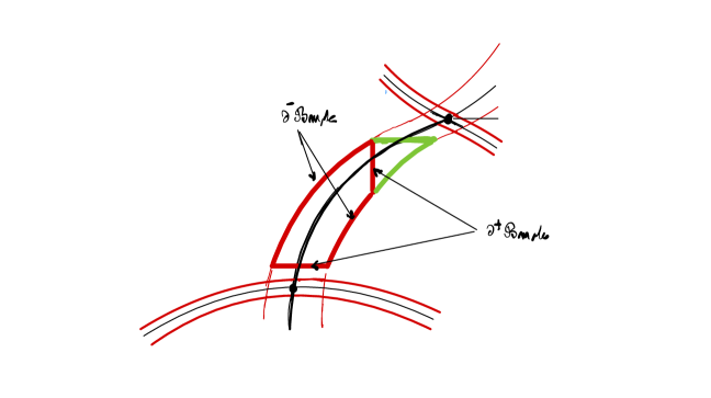
Figure 3. Interpretation of the resonant blocks in the light of Conley’s theory

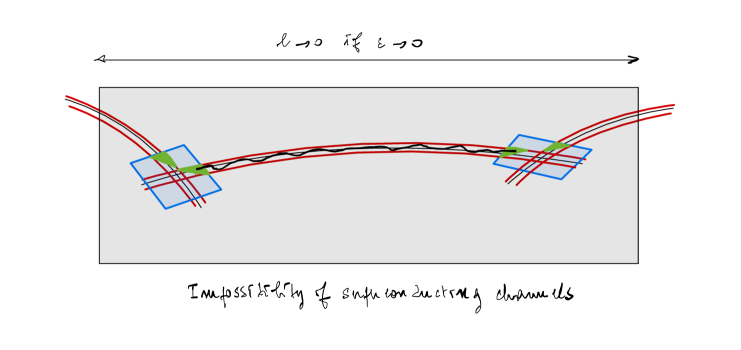
Figure 4. The Steepness property prevents the existence of superconductivity channels by ensuring a contact of finite order between the resonant manifold and the plane of fast drift. Here in the figure, $\ell$ is the size of the resonant zone (see Section 5.1)

Going back to the construction of Nekhoroshev’s patchwork, we have to make precise the process conducting to the enlargement of a block and its stability property. Here we will again make a crucial use of the fact that an orbit starting from an initial condition $I:=I(0)$ located in ${\mathcal{B}}_{m,p}$ will remain extremely close to the fast drift space $I+\rm Vect\,\Lambda$ for $0\leq t\leq T(\varepsilon)$, as long as it stays inside the resonant neighborhood ${\mathcal{M}}_{\Lambda}$ and far enough to the higher multiplicity resonance zones. Hence, to enlarge the block ${\mathcal{B}}_{m,k}$, we just have to add to it the collection of all the parts of the disks centered at points $I\in{\mathcal{B}}_{m,p}$ which are contained in the intersection of the fast drift spaces $I+\rm Vect\,\Lambda$ with the resonant neighborhood ${\mathcal{M}}_{\Lambda}$ (the resulting added subset is the green part in the previous two figures). We have in fact to add a very small neighborhood of these union of disks, in order to prevent the solutions to exit the extended block under the influence of the remainder part ${\mathcal{R}}$ of the dynamics during the time $T(\varepsilon)$, but this would not change our description significantly. Finally, one has to make sure that the extension will not intersect any other block of the same neighborhood ${\mathcal{B}}_{\Lambda}$ or any other resonance neighborhood, which can be done by a careful tuning of the width of the zone (see Section 5).

This concludes our description of Nekhoroshev’s method.

3. Functional setting

For $n\geq 1$, we denote the standard $n$-dimensional torus by $\mathbb{T}^{n}=\mathbb{R}^{n}/2\pi\mathbb{Z}^{n}$ and the standard $2n$-dimensional annulus by $\mathbb{A}^{n}=\mathbb{R}^{n}\times\mathbb{T}^{n}$.

1.  Hölder differentiable functions. Given an integer $q\geq 0$ and an open subset $D$ of $\mathbb{R}^{n}$, we denote by $C^{q}(D)$ the set of $q$-times continuously differentiable maps $f:D\to\mathbb{R}$ ($C^{0}(D)$ being the set of continuous functions on $D$). We identify $C^{q}(\mathbb{T}^{n})$ with the subset of $C^{q}(\mathbb{R}^{n})$ formed by the functions that are $2\pi\mathbb{Z}^{n}$-periodic and $C^{q}(D\times\mathbb{T}^{n})$ with the subset of $C^{q}(D\times\mathbb{R}^{n})$ formed by the functions which are $2\pi\mathbb{Z}^{n}$-periodic with respect to their last $n$ variables.

We use the conventional notation for partial derivatives: given $f\in C^{q}(D)$ and $\alpha\in{\mathbb{N}}^{n}$, we set for $x\in D$:

$$\partial^{\alpha}f(x)=\frac{\partial^{|\alpha|}f}{\partial x_{1}^{\alpha_{1}}\ldots\partial x_{n}^{\alpha_{n}}}(x),$$

with $|\alpha|=\alpha_{1}+\cdots+\alpha_{n}$.

We denote by $C_{b}^{q}(D)$ the set of $f\in C^{q}(D)$ such that

(3.1) $$\left\lVert f\right\rVert_{C^{q}(D)}:=\sup_{{\left|\alpha\right|}\leq q}\,\sup_{x\in D}{\left|\partial^{\alpha}f(x)\right|}<+\infty,$$

so that $\big{(}C_{b}^{q}(D),\left\lVert\cdot\right\rVert_{C^{q}(D)}\big{)}$ is a Banach space with multiplicative norm. It is understood that, for a function defined on a compex domain $D$, the $\left\lVert\cdot\right\rVert_{C^{0}(D)}$ is the usual sup-norm.

If $\ell>0$ is a non-integer real number, we write $q:=\lfloor\ell\rfloor$ for its integer part and $\mu=\ell-q\in(0,1)$ for its fractional part. Given a non-negative integer $q$ and $\mu\in(0,1)$, we denote by $C_{b}^{q,\mu}(D)$ the space formed by those functions $f\in C^{q}(D)$ such that

(3.2) $$\begin{split}|f|_{C^{q,\mu}(D)}:=\left\lVert f\right\rVert_{C^{q}(D)}+\sup_{\alpha\in\mathbb{N}^{n}:|\alpha|=q}\ \ \sup_{\begin{subarray}{c}x,y\in D:\\ 0<|x-y|<1\end{subarray}}\frac{|\partial^{\alpha}f(x)-\partial^{\alpha}f(y)|}{|x-y|^{\mu}}<+\infty.\end{split}$$

It is well-known that $\big{(}C_{b}^{q,\mu}(D),|\cdot|_{C^{q,\mu}(D)}\big{)}$ is also a Banach space with multiplicative norm. Functions belonging to these spaces are called Hölder-differentiable functions.

Given a non-integer real number $\ell>0$, together with its integer part $q:=\lfloor\ell\rfloor$ and its fractional part $\mu=\ell-q\in(0,1)$, we also write $C^{\ell}_{b}(D)$ instead of $C_{b}^{q,\mu}(D)$ and $|\cdot|_{C^{\ell}(D)}$ instead of $|\cdot|_{C^{q,\mu}(D)}$. Clearly $C^{\ell}_{b}(D)\subset C^{\ell^{\prime}}_{b}(D)$ when $\ell\geq\ell^{\prime}$ and if $f\in C^{\ell}_{b}(D)$

(3.3) $$|f|_{C^{\ell^{\prime}}(D)}\leq|f|_{C^{\ell}(D)}.$$

2.  Domains and their complex extensions.

Let us define the complex $n$-dimensional torus $\mathbb{T}_{\mathbb{C}}^{n}$ and the complex $2n$-dimensional annulus $\mathbb{A}_{\mathbb{C}}^{n}$ as

(3.4) $$\mathbb{T}^{n}_{\mathbb{C}}=\mathbb{C}^{n}/2\pi\mathbb{Z}^{n}\qquad\text{and}\qquad\mathbb{A}^{n}_{\mathbb{C}}=\mathbb{C}^{n}\times\mathbb{T}^{n}_{\mathbb{C}}.$$

We use angle coordinates $\theta$ on $\mathbb{T}^{n}_{\mathbb{C}}$ (with the usual abuse $\theta\in\mathbb{C}^{n}$ when there is no ambiguity) and action-angle coordinates $(I,\theta)$ on $\mathbb{A}_{\mathbb{C}}^{n}$. We see $\mathbb{T}^{n}_{\mathbb{C}}$ as a real $n$-dimensional vector bundle over $\mathbb{T}^{n}$. Consequently, we write

(3.5) $${\left|\theta\right|}:=\max_{j}{\left({\left|\operatorname{Im}\theta_{j}\right|}\right)}\ ,\qquad{\left|I\right|}:=\max_{j}{\left|I_{j}\right|}\ ,\qquad{\left|(I,\theta)\right|}=\max{\left({\left|I\right|},{\left|\theta\right|}\right)}\,.$$

For integer vectors $k\in\mathbb{Z}^{n}$, we use the “dual” $\ell^{1}$-norm, which we write $|k|$ only when there is no risk of confusion.

We need to introduce specific domains in $\mathbb{A}^{n}_{\mathbb{C}}$. First, given $r>0$, for a domain $D\subset\mathbb{R}^{n}$, we set

(3.6) $$D_{r}:=\big{\{}z\in\mathbb{C}^{n}:\exists z^{*}\in D:|z-z^{*}|_{2}<r\big{\}}\ .$$

As for the torus, given $s>0$, we introduce the global complex neighborhood

(3.7) $$\mathbb{T}^{n}_{s}:=\big{\{}\theta\in\mathbb{T}^{n}_{\mathbb{C}}\,:\,|\theta|<s\big{\}}.$$

We will essentially deal with complex domains of the form

(3.8) $${\mathcal{D}}_{r,s}\ :=D_{r}\times\mathbb{T}^{n}_{s}\subset\mathbb{A}_{\mathbb{C}}^{n}.$$

We finally write $D^{\mathbb{R}}_{r}$ and ${\mathcal{D}}_{r,s}^{\mathbb{R}}$ for the projections of $D_{r}$ and ${\mathcal{D}}_{r,s}$ on $\mathbb{R}^{n}$ and $\mathbb{A}^{n}$ respectively.

3.  Analytic functions and norms. If $g$ is a bounded holomorphic function defined on $\mathbb{T}^{n}_{s},D_{r}$ or ${\mathcal{D}}_{r,s}$ we denote the corresponding classical sup-norms by

(3.9) $${\left|g\right|}_{s}=\sup_{\theta\in\mathbb{T}^{n}_{s}}{\left|g(\theta)\right|},\quad{\left|g\right|}_{r}=\sup_{I\in D_{r}}{\left|g(I)\right|},\quad{\left|g\right|}_{r,s}=\sup_{(I,\theta)\in{\mathcal{D}}_{r,s}}{\left|g(I,\theta)\right|}.$$

Fix a bounded holomorphic function $g:{\mathcal{D}}_{r,s+2\sigma}\to\mathbb{C}$, where $\sigma>0$, and let $g(I,\theta)=\sum_{k\in\mathbb{Z}^{n}}\hat{g}_{k}(I)e^{{\rm i}\,k\cdot\theta}$ be its Fourier expansion, where $k\cdot\theta=k_{1}\theta_{1}+\cdots+k_{n}\theta_{n}$. We then introduce the weighted Fourier norm

(3.10) $$\left|\left|g\right|\right|_{r,s}:=\sup_{I\in D_{r}}\sum_{k\in\mathbb{Z}^{n}}{\left|\hat{g}_{k}(I)\right|}\,e^{{\left|k\right|}s},$$

which is finite and satisfies

(3.11) $${\left|g\right|}_{r,s}\leq\left|\left|g\right|\right|_{r,s}\leq{\rm coth^{n}\,}\sigma\,{\left|g\right|}_{r,s+\sigma}.$$

We denote by ${\mathcal{A}}_{r,s}$ the space of holomorphic functions on ${\mathcal{D}}_{r,s}$ with finite Fourier norm. Endowed with this norm, ${\mathcal{A}}_{r,s}$ is a Banach algebra.

Finally, the norm of a vector valued function will be the maximum of the norms of its components.

4. Analytic smoothing

We state in this section the key ingredient of the present work. We first recall the analytic smoothing method as developed by Jackson-Moser-Zehnder for Hölder functions of $\mathbb{R}^{n}$: given a Hölder function $f\in C^{\ell}(\mathbb{R}^{n})$ and a positive number $s\leq 1$, this yields an analytic function on the complex neighborhood $\mathbb{R}^{n}_{s}$ whose restriction to $\mathbb{R}^{n}$ is close to $f$ in the $C^{k}$ topology, for $1\leq k\leq\ell$.

We then adapt their method to our specific setting of functions defined on $\mathbb{A}^{n}$ (see Section 4.2) and, in addition, we derive the new estimate (4.22) for the weighted Fourier norm of the smoothed function.

4.1. Analytic smoothing in $\mathbb{R}^{n}$

We recall here the result by Jackson, Moser and Zehnder, following the presentation by [9] and [24].

Proposition 4.1 (Jackson-Moser-Zehnder).

Fix an integer $n\geq 1$, a real number $\ell>0$ and let $f\in C^{\ell}_{b}(\mathbb{R}^{n})$. Then there is a constant ${\mathtt{C}}_{\mathtt{J}}={\mathtt{C}}_{\mathtt{J}}(\ell,n)$ such that for every $0<s\leq 1$ there exists a function ${\mathtt{f}}_{s}$, analytic on $\mathbb{R}^{n}_{s}$, which satisfies

(4.1) $$\left|\partial^{\alpha}{\mathtt{f}}_{s}(x)-\sum_{\begin{subarray}{c}\beta\in\mathbb{N}^{n}:|\beta|\leq\lfloor\ell\rfloor-|\alpha|\end{subarray}}\partial^{\alpha+\beta}f(\operatorname{Re}x)\frac{(\operatorname{Im}x)^{\beta}}{\beta!}\right|\leq{\mathtt{C}}_{\mathtt{J}}\,s^{\ell-|\alpha|}{\left|f\right|}_{C^{\ell}(\mathbb{R}^{n})},\quad\forall x\in\mathbb{R}^{n}_{s},$$

for all multi-integer $\alpha\in{\mathbb{N}}^{n}$ such that ${\left|\alpha\right|}\leq\lfloor\ell\rfloor$. More precisely, given any even $C^{\infty}$ function $\Phi$ with compact support in $\mathbb{R}^{n}$ and setting

(4.2) $$K(\xi):=\frac{1}{(2\pi)^{n}}\int_{\mathbb{R}^{n}}\Phi(x)e^{{\rm i}x\cdot\xi}dx,\quad\xi\in\mathbb{R}^{n}_{s},$$

the function

(4.3) $${\mathtt{f}}_{s}(x):=\int_{\mathbb{R}^{n}}{K}\left(\frac{x}{s}-\xi\right)f(s\xi)\ d\xi\ ,$$

satisfies the previous requirements (where the constant ${\mathtt{C}}_{\mathtt{J}}(\ell,n)$ depends on the choice of $\Phi$).

Observe that ${\mathtt{f}}_{s}$ takes real values when its argument is in $\mathbb{R}^{n}$.

4.2. Analytic smoothing in $\mathbb{A}^{n}$.

In the following, the Hölder regularity $\ell$ is assumed to satisfy $\lfloor\ell\rfloor\geq n+1$ as in the hypotheses of Theorem 1.1.
We now specialize the previous result to our setting and give a more detailed description of the method in the case of functions of $\mathbb{A}^{n}$. In that case, the analytic smoothing is a truncation of the Fourier series of the initial Hölder function with suitably modified Fourier coefficients (the so-called Jackson polynomials). Our main concern here is to derive an estimate on the weighted Fourier norm of an $s$-smoothed $C^{\ell}$ function over a complex strip of width $s$.

To make the whole presentation more explicit and take the anisotropy of the weighted Fourier norm into account, we first consider functions defined on $\mathbb{R}^{n}$ and $\mathbb{T}^{n}$ separately. This then yields a statement for functions of $\mathbb{A}^{n}$.

$\bullet$ The non-periodic case. Fix an even function $\Phi:\mathbb{R}^{n}\to[0,1]$, of class $C^{\infty}$, with support in the ball $\overline{B}_{2}(0,1)$ and let $K:\mathbb{C}^{n}\to\mathbb{C}$ be its Fourier-Laplace transform:

(4.4) $$K(y)=\frac{1}{(2\pi)^{n}}\int_{\mathbb{R}^{n}}\Phi(\eta)e^{-i\eta\cdot y}d\eta.$$

Since $\Phi$ is compactly supported, then $K$ is an entire function . Moreover its restriction to $\mathbb{R}^{n}$ is in the Schwartz class ${\mathcal{S}}(\mathbb{R}^{n})$ since $\Phi$ is, and this is also the case for the translates $y\mapsto K(y-z)$ for $y\in\mathbb{R}^{n}$ and fixed $z\in\mathbb{C}^{n}$.

Let $f:\mathbb{R}^{n}\to\mathbb{R}$ be a $C^{\ell}$ function with $\lfloor\ell\rfloor\geq n+1$, with compact support contained in the ball $\overline{B}_{\infty}(0,R_{0})$ for some $R_{0}>0$. Given $s\in\,]0,1]$, set for $x\in\mathbb{R}^{n}$:

(4.5) $${\bf f}_{s}(x)=\frac{1}{s^{n}}\int_{\mathbb{R}^{n}}K\Big{(}\frac{x-y}{s}\Big{)}f(y)dy=\int_{\mathbb{R}^{n}}K\Big{(}\frac{x}{s}-y\Big{)}f(sy)dy=\int_{\mathbb{R}^{n}}K(y)f(x-sy)dy.$$

By Fourier reciprocity:

$${\bf f}_{s}(x)=\int_{\mathbb{R}^{n}}\Phi(\eta)\widehat{f(x-sy)}(\eta)d\eta,$$

with:

$$\widehat{f(x-sy)}(\eta)=\frac{1}{(2\pi)^{n}}\int_{\mathbb{R}^{n}}f(x-sy)e^{-iy\cdot\eta}dy=\frac{1}{(2\pi)^{n}s^{n}}\int_{\mathbb{R}^{n}}f(u)e^{-i(x-u)\cdot\eta/s}du=\frac{e^{-ix\cdot\eta/s}}{s^{n}}\widehat{f}\Big{(}\frac{-\eta}{s}\Big{)}.$$

Therefore, since $\Phi$ is even:

(4.6) $${\bf f}_{s}(x)=\frac{1}{s^{n}}\int_{\mathbb{R}^{n}}\Phi(\eta)\widehat{f}\Big{(}\frac{-\eta}{s}\Big{)}e^{-ix\cdot\eta/s}d\eta=\int_{\mathbb{R}^{n}}\Phi(s\eta)\widehat{f}({-\eta})e^{-ix\cdot\eta}d\eta=\int_{\mathbb{R}^{n}}\Phi(s\eta)\widehat{f}({\eta})e^{ix\cdot\eta}d\eta.$$

Hence ${\bf f}_{s}$ is the inverse Fourier-Laplace transform of the “truncation”

$$\eta\mapsto\Phi(s\eta)\widehat{f}(\eta).$$

The first term of (4.5) shows that ${\bf f}_{s}$ extends to $\mathbb{C}^{n}$ and is an entire function. To get our final estimate we go back to the second term in (4.5), which yields

(4.7) $$|{\bf f}_{s}(z)|\leq\left\lVert f\right\rVert_{C^{0}(\mathbb{R}^{n})}\int_{\mathbb{R}^{n}}\left|K\left(\frac{z}{s}-y\right)\right|dy,\qquad z\in\mathbb{C}^{n}.$$

By the Schwartz estimate of Lemma A.1, there exists a constant $C_{n}$ such that

$$\left|K\left(\frac{z}{s}-y\right)\right|\leq C_{n}\frac{e^{\operatorname{Im}(z/s-y)}}{(1+|z/s-y|_{2})^{n+1}},$$

so that, for $y\in\mathbb{R}^{n},z\in\mathbb{C}^{n}$ and $|\operatorname{Im}z|_{2}\leq s$:

$$\left|K\left(\frac{z}{s}-y\right)\right|\leq C_{n}\frac{e}{(1+|\operatorname{Re}(z/s-y)|_{2})^{n+1}}.$$

Hence:

(4.8) $$|{\bf f}_{s}(z)|\leq\left\lVert f\right\rVert_{C^{0}(\mathbb{R}^{n})}C_{n}e\int_{\mathbb{R}^{n}}\frac{dy}{(1+|y|_{2})^{n+1}}.$$

since $z/s$ is fixed and can be eliminated by a simple translation. We finally get the following estimate:

(4.9) $$|{\bf f}_{s}|_{s}=\sup_{z\in\mathbb{C}^{n}:{\left|\operatorname{Im}z\right|}_{2}\leq s}|{\bf f}_{s}(z)|\leq C_{1}(n)\left\lVert f\right\rVert_{C^{0}(\mathbb{R}^{n})},$$

with

$$C_{1}(n):=C_{n}e\int_{\mathbb{R}^{n}}\frac{dy}{(1+|y|_{2})^{n+1}}<\infty.$$

$\bullet$ The periodic case. Fix now an even function $\Psi:\mathbb{R}^{n}\to[0,1]$, of class $C^{\infty}$, with support in the ball $\overline{B}_{1}(0,1)$ and define the associate kernel $K$ as in (4.4).

Fix a ${2\pi}\mathbb{Z}^{n}$-periodic function $f\in C^{\ell}(\mathbb{R}^{n})$ with $\ell\geq n+1$. Then the Fourier expansion

$$f(\theta)=\sum_{k\in\mathbb{Z}^{n}}\widehat{f}_{k}e^{ik\cdot\theta},\qquad\widehat{f}_{k}=\frac{1}{(2\pi)^{n}}\int_{\mathbb{T}^{n}}f(\varphi)e^{-ik\cdot\varphi}d\varphi,$$

converges normally since, by Lemma A.2 in Appendix A, for $k\in\mathbb{Z}^{n}\setminus\{0\}$, there exists a universal constant ${\mathtt{C}}_{\mathtt{F}}(n,\ell)$ satisfying

(4.10) $${\left|\widehat{f}_{k}\right|}\leq{\mathtt{C}}_{\mathtt{F}}(n,\ell)\frac{||f||_{C^{\lfloor\ell\rfloor}}}{{\left|k\right|}_{\infty}^{\lfloor\ell\rfloor}}$$

and $\lfloor\ell\rfloor\geq n+1$ by hypothesis. For $s\in\,]0,1]$, the function

$${\bf f}_{s}(\theta)=\frac{1}{s^{n}}\int_{\mathbb{R}^{n}}K\Big{(}\frac{\theta-\varphi}{s}\Big{)}f(\varphi)d\varphi$$

is well-defined and, by the Fubini interversion theorem:

$${\bf f}_{s}(\theta)=\sum_{k\in\mathbb{Z}^{n}}\widehat{f}_{k}\int_{\mathbb{R}^{n}}K(\varphi)e^{ik\cdot(\theta-s\varphi)}d\varphi=\sum_{k\in\mathbb{Z}^{n}}\widehat{f}_{k}e^{ik\cdot\theta}\int_{\mathbb{R}^{n}}K(\varphi)e^{-isk\cdot\varphi}d\varphi.$$

Hence, since $K$ is the inverse Fourier transform of $\Psi$, by the Fourier inversion theorem:

(4.11) $${\bf f}_{s}(\theta)=\sum_{k\in\mathbb{Z}^{n}}\widehat{f}_{k}\Psi(sk)\,e^{ik\cdot\theta},\quad\theta\in\mathbb{R}^{n}.$$

As in the non-periodic case, this makes apparent that ${\bf f}_{s}$ is a continuous truncation of the Fourier expansion of $f$ with a $\Psi$-dependent modification of its Fourier coefficients (the so-called Jackson polynomial):

(4.12) $$\widehat{({\bf f}_{s})}_{k}=\Psi(sk)\widehat{f}_{k}\ .$$

Consequently, the Fourier norm

$$\left\lVert{\bf f}_{s}\right\rVert_{s}=\sum_{k\in\mathbb{Z}^{n}}{\left|\widehat{({\bf f}_{s})}_{k}\right|}e^{s{\left|k\right|}_{1}}$$

depends only on the harmonics such that $|k|_{1}\leq 1/s$ and satisfies

$$\left\lVert{\bf f}_{s}\right\rVert_{s}\leq\sum_{{\left|k\right|}_{1}\leq 1/s}{\left|\widehat{({\bf f}_{s})}_{k}\right|}\,e^{s{\left|k\right|}_{1}}\leq e\sum_{{\left|k\right|}_{1}\leq 1/s}{\left|\widehat{({\bf f}_{s})}_{k}\right|}\leq e\,\sum_{k\in\mathbb{Z}^{n}}{\left|\widehat{f}_{k}\right|}.$$

Hence, by (4.10):

(4.13) $$\left\lVert{\bf f}_{s}\right\rVert_{s}\leq C_{2}(\ell){\left|f\right|}_{C^{\lfloor\ell\rfloor}}$$

with

(4.14) $$C_{2}(\ell):=e\Bigg{(}1+{\mathtt{C}}_{\mathtt{F}}(n,\ell)\sum_{k\in\mathbb{Z}^{n}\setminus\{0\}}\frac{1}{{\left|k\right|}_{\infty}^{[\ell]}}\Bigg{)}$$

$\bullet$ Functions on $\mathbb{A}^{n}$. We finally gather together the previous two cases. Let $\Phi\otimes\Psi:\mathbb{R}^{n}\times\mathbb{R}^{n}\to[0,1]$ be defined by

$$\Phi\otimes\Psi(x,\theta)=\Phi(x)\Psi(\theta),$$

and define the kernel

$$K(y,\varphi)=\int_{\mathbb{R}^{2n}}\Phi\otimes\Psi(x,\theta)\,e^{-i(x,\theta)\cdot(y,\varphi)}\,dxd\theta=K_{\Phi}(y)K_{\Psi}(\varphi)=K_{\Phi}\otimes K_{\Psi}(y,\varphi)$$

where $K_{\Phi}$ and $K_{\Psi}$ are defined as above. Fix a function $f:\mathbb{R}^{n}\times\mathbb{R}^{n}\to\mathbb{C}$, $2\pi\mathbb{Z}^{n}$-periodic with respect to its last $n$ variables, with support in $\overline{B}_{2}(0,R_{0})\times\mathbb{R}^{n}$ for some $R_{0}>0$, belonging to $C^{\ell}(\mathbb{R}^{2n})$ with $\lfloor\ell\rfloor\geq n+1$. For $s\in\,]0,1]$ and $(x,\theta)\in\mathbb{R}^{n}\times\mathbb{R}^{n}$, set

$$\begin{array}[]{lll}{\bf f}_{s}(x,\theta)&\!\!\!=\displaystyle\int_{\mathbb{R}^{2n}}K(y,\varphi)f(x-sy,\theta-s\varphi)dyd\varphi\\[9.0pt] &\!\!\!=\displaystyle\int_{\mathbb{R}^{2n}}K(y,\varphi)\sum_{k\in\mathbb{Z}^{n}}\widehat{f}_{k}(x-sy)e^{ik\cdot(\theta-s\varphi)}dyd\varphi\\[9.0pt] \end{array}$$

with

(4.15) $$\widehat{f}_{k}(u)=\frac{1}{(2\pi)^{n}}\int_{\mathbb{T}^{n}}f(u,v)e^{-ik\cdot v}dv.$$

Note that $f_{k}$ is $C^{\ell}$, with support in $\overline{B}_{2}(0,R_{0})$, so that the previous study on the non-periodic case applies to $f_{k}$. By Fubini interversion

(4.16) $$\begin{array}[]{lll}{\bf f}_{s}(x,\theta)&\!\!\!=\displaystyle\sum_{k\in\mathbb{Z}^{n}}\int_{\mathbb{R}^{2n}}K(y,\varphi)\widehat{f}_{k}(x-sy)e^{ik\cdot(\theta-s\varphi)}dyd\varphi\\[9.0pt] &\!\!\!=\displaystyle\sum_{k\in\mathbb{Z}^{n}}\Big{(}\int_{\mathbb{R}^{n}}K_{\Phi}(y)\widehat{f}_{k}(x-sy)dy\Big{)}\Big{(}\int_{\mathbb{R}^{n}}K_{\Psi}(\varphi)e^{ik\cdot(\theta-s\varphi)}d\varphi\Big{)}\\[12.0pt] &\!\!\!=\displaystyle\sum_{k\in\mathbb{Z}^{n}}({\bf\widehat{f}}_{k})_{s}(x)\Psi(sk)e^{ik\cdot\theta}\\[10.0pt] \end{array}$$

where $({\bf\widehat{f}}_{k})_{s}$ stands for the analytic smoothing of the Fourier coefficient $\widehat{f}_{k}$. This proves that the Fourier coefficient $(\widehat{{\bf f}}_{s})_{k}(x)$ relative to the periodic variable $\theta$ reads

(4.17) $$(\widehat{\bf f}_{s})_{k}(x)=\Psi(sk)({\bf\widehat{f}}_{k})_{s}(x),\quad k\in\mathbb{Z}^{n}.$$

Expressions (4.16) and (4.17) make clear that the whole smoothing procedure of a function depending both on action and angle variables consists in constructing a Jackson trigonometric polynomial by smoothing the Fourier coefficients and by suitably truncating the Fourier series.

Using the definition of $\Psi$, $(\widehat{\bf f}_{s})_{k}=0$ when ${\left|k\right|}_{1}>1/s$ and, by (4.17) and (4.9):

(4.18) $$|(\widehat{\bf f}_{s})_{k}(z)|\leq|(\widehat{\bf f}_{k})_{s}(z)|\leq C_{1}(n)\left\lVert\widehat{f}_{k}\right\rVert_{C^{0}(\mathbb{R}^{n})}\leq C_{1}(n){\mathtt{C}}_{\mathtt{F}}(n,\ell)\frac{|f|_{C^{\lfloor\ell\rfloor}(\mathbb{R}^{n})}}{|k|_{\infty}^{\lfloor\ell\rfloor}},\quad k\neq 0,\ {\left|k\right|}_{1}\leq 1/s,$$

and

(4.19) $$|(\widehat{\bf f}_{s})_{0}(z)|\leq C_{1}(n)\left\lVert\widehat{f}_{0}\right\rVert_{C^{0}(\mathbb{R}^{n})}\leq C_{1}(n)\left\lVert f\right\rVert_{C^{0}(\mathbb{R}^{n})}.$$

As for the weighted Fourier norm of ${\bf f}_{s}$, we finally get:

$$\begin{array}[]{lll}||{\bf f}_{s}||_{s,s}&=&\sup_{{\left|\operatorname{Im}z\right|}_{2}\leq s}\sum_{k\in\mathbb{Z}^{n}}{\left|(\widehat{\bf f}_{s})_{k}(z)\right|}\,e^{s{\left|k\right|}_{1}}\\[8.0pt] &\leq&C_{1}(n)\left\lVert f\right\rVert_{C^{0}(\mathbb{R}^{n})}+\displaystyle\sum_{\begin{subarray}{c}k\in\mathbb{Z}^{n}\backslash\{0\}:\\ |k|_{1}\leq 1/s\end{subarray}}eC_{1}(n){\mathtt{C}}_{\mathtt{F}}(n,\ell)\frac{|f|_{C^{\lfloor\ell\rfloor}(\mathbb{R}^{n})}}{|k|_{\infty}^{\lfloor\ell\rfloor}}\leq C_{L}(n,\ell)|f|_{C^{\ell}(\mathbb{R}^{n})}\,,\end{array}$$

where

(4.20) $$C_{L}(n,\ell):=C_{1}(n)\left(1+e{\mathtt{C}}_{\mathtt{F}}(n,\ell)\sum_{k\in\mathbb{Z}^{n}}\frac{1}{|k|_{\infty}^{\lfloor\ell\rfloor}}\right)<+\infty.$$

4.3. The main result with an application to normal forms.

4.3.1. Main result

Gathering together the elements of the previous section, we get the following result.

Theorem 4.1 (Analytic smoothing).

Fix an integer $n\geq 1$, $R>0$ and $s\in\,]0,1]$. Let $f$ be a $C^{\ell}$ function on $B_{\infty}(0,2R)\times\mathbb{T}^{n}$. Then there exist two constants ${\mathtt{C}}_{A}(R,\ell,n),{\mathtt{C}}_{B}(R,\ell,n)$ and an analytic function ${\mathtt{f}}_{s}$ on the set $\mathbb{A}_{s}^{n}$ satisfying

(4.21) $$\left\lVert f-\mathtt{f}_{s}\right\rVert_{C^{p}(B_{\infty}(0,R)\times\mathbb{T}^{n})}\leq\ {\mathtt{C}}_{A}(R,\ell,n)\ s^{\ell-p}|f|_{C^{\ell}(B_{\infty}(0,2R)\times\mathbb{T}^{n})}\quad\text{ for any integer $0\leq p\leq\lfloor\ell\rfloor$}$$

and

(4.22) $$\left\lVert{\mathtt{f}}_{s}\right\rVert_{s,s}\leq{\mathtt{C}}_{B}(R,\ell,n){|f|_{C^{\ell}(B_{\infty}(0,2R)\times\mathbb{T}^{n})}}.$$

Moreover, $\mathtt{f}_{s}$ is a trigonometric polynomial in the angular variables.

Proof.

Fix a function $\chi\in C^{\infty}(\mathbb{R}^{n})$, with values in $[0,1]$, equal to $1$ on the ball $B_{\infty}(0,R)$ and with support in $B_{\infty}(0,2R)$. Then the product $\overline{f}:=\chi f$ is $C^{\ell}$ on $\mathbb{A}^{n}$, has compact support in $B_{\infty}(0,2R)\times\mathbb{T}^{n}$ and coincides with $f$ on $B_{\infty}(0,R)\times\mathbb{T}^{n}$. Moreover

$$|\overline{f}|_{C^{\ell}(B_{\infty}(0,2R)\times\mathbb{T}^{n})}\leq{{\mathtt{C}}_{K}}|f|_{C^{\ell}(B_{\infty}(0,2R)\times\mathbb{T}^{n})}$$

where ${{\mathtt{C}}_{K}}=C|\chi|_{C^{\ell}(B_{\infty}(0,R)\times\mathbb{T}^{n})}$ and $C$ is a universal constant. By the Jackson-Moser-Zehnder theorem applied to $\overline{f}$, there is an analytic function $\mathtt{\bar{f}}_{s}$ on $\mathbb{A}^{n}_{s}$ satisfying

(4.23) $$\left|\partial^{\alpha}\mathtt{\bar{f}}_{s}(I,\theta)-\sum_{\begin{subarray}{c}\beta\in\mathbb{N}^{2n}:\\ |\beta|\leq\lfloor\ell\rfloor-|\alpha|\end{subarray}}\partial^{\alpha+\beta}\bar{f}(\operatorname{Re}(I,\theta))\frac{(\operatorname{Im}(I,\theta))^{\beta}}{\beta!}\right|\leq{\mathtt{C}}_{\mathtt{J}}s^{{\ell}-|\alpha|}|\bar{f}|_{C^{\ell}(\mathbb{A}^{n})},$$

so that for any $p\leq\lfloor\ell\rfloor$:

(4.24) $$\left\lVert\bar{f}-\mathtt{\bar{f}}_{s}\right\rVert_{C^{p}(\mathbb{A}^{n})}\leq\ {\mathtt{C}}_{\mathtt{J}}s^{\ell-p}|\bar{f}|_{C^{\ell}(\mathbb{A}^{n})}.$$

As a consequence, taking the form of $\chi$ into account, one gets

(4.25) $$\left\lVert{f}-\mathtt{f}_{s}\ \right\rVert_{C^{p}(B_{\infty}(0,R)\times\mathbb{T}^{n})}\leq{{\mathtt{C}}_{K}}{\mathtt{C}}_{\mathtt{J}}s^{\ell-p}|f|_{C^{\ell}(B_{\infty}(0,2R)\times\mathbb{T}^{n})}.$$

Setting ${\mathtt{C}}_{A}:={{\mathtt{C}}_{K}}{\mathtt{C}}_{\mathtt{J}}$ and, since the analyticity width $\rho$ of the integrable part $h$ is greater than $s$, the bound (4.21) follows. The proof of (4.22) is an immediate consequence of the previous paragraphs if one sets ${\mathtt{C}}_{B}:=C_{L}\times C_{K}$. ∎

4.3.2. An easy way to derive normal forms for Hölder functions from analytic ones.

Let us now explain our strategy for a general Hölder Hamiltonian, we will then restrict ourselves to the case where $h$ is analytic. Let

(4.26) $$H(I,\theta):=h(I)+f(I,\theta)$$

be $C^{\ell}$ on $B_{\infty}(0,2R)\times\mathbb{T}^{n}$. Given $s\in\,]0,1]$, let ${\bf H}_{s}$ be the $s$-smoothed analytic function given by Theorem 4.1 applied to the function $H$. By classical constructions (alluded to in the introduction and which will be recalled in the following), there exist (close to identity) symplectic analytic local diffeomorphisms $\Psi$ defined on domains $D\subset\mathbb{A}^{n}$ which bring ${\bf H}_{s}={\bf h}_{s}+{\bf f}_{s}$ to the normal form ${\bf H}_{s}\circ\Psi:D\to\mathbb{R}$:

(4.27) $${\bf H}_{s}\circ\Psi={\bf h}_{s}+\bf{g}+{\bf f}_{s}^{*}$$

where ${\bf h}_{s}$ is nothing else than the smoothed initial integrable Hamiltonian, ${\mathtt{g}}$ is a resonant part which controls the fast drift in certain directions and ${\bf f}_{s}^{*}$ is a very small remainder – all these functions being analytic on $D$. The keypoint in our subsequent constructions is the following very simple equality

(4.28) $$H\circ\Psi={\bf H}_{s}\circ\Psi+(H-{\bf H}_{s})\circ\Psi={\bf h}_{s}+\bf{g}+\big{[}{\bf f}_{s}^{*}+(H-{\bf H}_{s})\circ\Psi\big{]}.$$

This is a normal form for $H$, obtained by composition of $H$ with an analytic diffeomorphism, in which the first three terms are analytic on $D$ and only the last one is $C^{\ell}$. So $H\circ\Psi$ has the same structure and dynamical interpretation as ${\bf H}_{s}\circ\Psi$, provided that the $C^{\ell}$ size of the additional remainder $(H-{\bf H}_{s})\circ\Psi$ is of the same order as the size of the initial remainder ${\bf f}_{s}^{*}$. This issue strongly depends on the analytic smoothing method in use, we will show in the sequel that the Jackson-Moser-Zehnder method is relevant for our purposes. Our study will be even easier since we assume from the beginning that the integrable part $h$ is analytic.

It turns out that the same smoothing method - and the same simple way to get a normal form from an analytical one - are also relevant in many other functional classes, the main ones being the Gevrey classes already used in [18], but also other ultradifferentiable ones. This will be developed in a further work.

5. Estimates of stability

The aim of this section is to prove Theorem 1.1. The proof consists of several steps. Following the discussion in section 2 of the introduction, we first build an appropriate resonant covering of the phase space for the integrable Hamiltonian $h$. Secondly, we study the local dynamics by applying Pöschel’s resonant normal form (see Appendix B) in each resonant block and we set the dependencies of the ultraviolet cut-off $K$ and analyticity widths $r,s$ on the perturbative parameter $\varepsilon$. Finally, we exploit the properties of the resonant covering and we obtain a global result of stability by exploiting the so called ”capture in resonance” argument.

5.1. Construction of the resonant patchwork

In the sequel, we follow ref. [13], in which the choices of the parameters and the dependencies of the small denominators on the ultraviolet cut-off $K$ are justified heuristically. For the sake of clarity, in order to have coherent notations we denote by $D_{\Lambda}$ rather than ${\mathcal{B}}_{\Lambda}$ the resonant blocks introduced in Section 2, moreover when possible we will not keep track of constants but rather indicate their presence in bounds and equalities by using the following symbols respectively: $\circeq,\lessdot$ and $\gtrdot$.

We start by setting some parameters, depending on the steepness indices ${\bm{\alpha}}_{1},..,{\bm{\alpha}}_{n-1}$ of $h$, that will be useful throughout this section.

(5.1) $$p_{j}:=\begin{cases}\Pi_{i=j}^{n-2}{\bm{\alpha}}_{i}&,\quad\text{if }j\in\{1,...,n-2\}\\ 1&,\quad\text{if }j\in\{n-1,n\}\end{cases}\ ;\quad q_{j}:=np_{j}-j\ ,\ \ j\in\{1,...,n\}\ ;\quad c_{j}:=q_{j}-q_{j+1}\ ,\ \ j\in\{1,...,n-1\}$$

and set

(5.2) $$a:=\frac{1}{2n{\bm{\alpha}}_{1}...{\bm{\alpha}}_{n-2}}=\frac{1}{2np_{1}}\quad,\qquad b:=\frac{1}{2n{\bm{\alpha}}_{1}...{\bm{\alpha}}_{n-1}}=\frac{a}{{\bm{\alpha}}_{n-1}}\quad,\qquad{\mathtt{R}}(\varepsilon):\circeq\,\varepsilon^{b}\ .$$

With this setting, we fix an action $I_{0}\in B_{\infty}(0,R/4)$ and we consider its neighborhood $B_{2}(I_{0},{\mathtt{R}}(\varepsilon))$.

Since $h$ is steep in $B_{\infty}(0,R)$, the norm of the frequency $\omega:=\partial_{I}h(I)$ at any point of this set admits a uniform lower positive bound, that is $\inf_{I\in B_{\infty}(0,R)}||\omega(I)||\gtrdot 1$. Hence, when studying the geography of resonances for $h$, for sufficiently small $\varepsilon$ and without any loss of generality we can just consider maximal lattices $\Lambda\subset\mathbb{Z}^{n}_{K}$ of dimension $j\in\{0,...,n-1\}$, with $K\geq 1$ the ultraviolet cut-off. For a lattice $\Lambda$ of dimension $j\in\{0,...,n-1\}$ we define its associated resonant zone as

(5.3) $$Z_{\Lambda}:=\{I\in B_{2}(I_{0},{\mathtt{R}}(\varepsilon)):\ \forall k\in\Lambda\ \text{one has }\ \ |k\cdot\omega(I)|<\delta_{\Lambda}\}\ ,\ \ \delta_{\Lambda}:\circeq\frac{1}{|\Lambda|K^{q_{j}}}\ .$$

and its associated resonant block $D_{\Lambda}$ as

(5.4) $$D_{\Lambda}:=Z_{\Lambda}\backslash\bigcup_{\Lambda^{\prime}:\,\dim\Lambda^{\prime}=j+1}Z_{\Lambda^{\prime}}\ .$$

Note that $D_{\Lambda}$ corresponds to that part of the resonant zone $Z_{\Lambda}$ which does not contain any other resonances other than the one associated to $\Lambda$. In particular, this implies that for the completely non-resonant block associated to $\Lambda=\{0\}$ and for any block $\Lambda$ corresponding to a maximal resonance of dimension $j=n-1$ one has, respectively

(5.5) $$D_{0}:=B(I_{0},{\mathtt{R}}(\varepsilon))\backslash\bigcup_{\Lambda^{\prime}:\ \dim\Lambda^{\prime}=1}Z_{\Lambda^{\prime}}\quad\text{ and }\quad D_{\Lambda}=Z_{\Lambda}\ .$$

For any $j\in\{0,...,n-1\}$ we set

(5.6) $$D_{j}:=\bigcup_{\Lambda:\ \dim\Lambda=j}D_{\Lambda}\quad,\qquad Z_{j}:=\bigcup_{\Lambda:\ \dim\Lambda=j}Z_{\Lambda}\ .$$

It is easy to see from (5.4) that

(5.7) $$D_{j}=Z_{j}\backslash Z_{j+1}$$

so that from the definition of $D_{0}$ in (5.5) one has the decompositions

(5.8) $$B_{2}(I_{0},{\mathtt{R}}(\varepsilon))=\bigcup_{i=0}^{n-1}D_{i}\quad,\qquad B_{2}(I_{0},{\mathtt{R}}(\varepsilon))=\left(\bigcup_{i=0}^{j-1}D_{i}\right)\cup Z_{j}\qquad\forall j=1,...,n-1\ .$$

As we have explained in the introduction (see section 2), a large drift over a short time of any action variable $I\in D_{\Lambda}$ is only possible along the plane of fast drift $I+\langle\Lambda\rangle$ spanned by the vectors belonging to $\Lambda$. Moreover, the fast motion of the orbit starting at $I$ along $I+\langle\Lambda\rangle$ can take the actions out of the block $D_{\Lambda}$. So, we are interested in understanding what happens when the actions leave $D_{\Lambda}$ but keep staying in $Z_{\Lambda}$. Hence, we are naturally taken to consider the intersection of a neighborhood of $I+\langle\Lambda\rangle$ with $Z_{\Lambda}$. In this spirit, we fix

(5.9) $$\rho(\varepsilon):=\displaystyle\frac{{\mathtt{R}}(\varepsilon)}{2n}$$

and, for any $0<\eta\leq\rho(\varepsilon)$ and for any action $I\in D_{\Lambda}$ with $\Lambda\neq\{0\}$, we define the disc associated to $I$ as

(5.10) $$\mathbf{D}^{\rho}_{\Lambda,\eta}(I):=\Bigg{(}\ \bigg{(}\bigcup_{I^{\prime}\in I+\langle\Lambda\rangle}B_{2}(I^{\prime},\eta)\bigg{)}\cap Z_{\Lambda}\cap B\big{(}I_{0},{\mathtt{R}}(\varepsilon)-\rho(\varepsilon)\big{)}\ \Bigg{)}_{I}$$

where the subscript $I$ denotes the connected component of the set containing the action $I$. Since we are going to study the fate of all orbits starting at a fixed block $D_{\Lambda}$, with $\Lambda\neq\{0\}$, that exit such block in a short time along the plane of fast drift, we are also led to define the extended resonant block

(5.11) $$D_{\Lambda,r_{\Lambda}}^{\rho}:=\Bigg{(}\bigcup_{I\in D_{\Lambda}\cap B(I_{0},{\mathtt{R}}(\varepsilon)-\rho(\varepsilon))}\mathbf{D}^{\rho}_{\Lambda,r_{\Lambda}}(I)\Bigg{)}\ \subset\ Z_{\Lambda}\cap B\big{(}I_{0},{\mathtt{R}}(\varepsilon)-\rho(\varepsilon)\big{)}\quad,\qquad r_{\Lambda}:=\frac{\delta_{\Lambda}}{M}\ ,$$

where $M$ was defined in $\eqref{M}$. In the same way, the extended non-resonant block is defined as

(5.12) $$D_{0}^{\rho}:=D_{0}\cap B(I_{0},{\mathtt{R}}(\varepsilon)-\rho(\varepsilon))\ .$$

5.2. The resonant blocks

As we have explained there, Nekhoroshev proved in [20] that, if $h$ is steep, when any action $I\in D_{\Lambda}$, with $\Lambda\neq\{0\}$, moves along the plane of fast drift, it must exit the resonant zone $Z_{\Lambda}$ after having travelled for a short distance. Indeed, if $h$ is steep with steepness indices ${\bm{\alpha}}_{1},...,{\bm{\alpha}}_{n-1}$ one can prove that the diameter of the intersection of a neighborhood of the fast drift plane with the resonant zone is small in the sense given by the following

Lemma 5.1.

For any $\Lambda\neq 0$, $\dim\Lambda=j\in\{1,...,n-1\}$, for any $I\in D_{\Lambda}\cap B(I_{0},{\mathtt{R}}(\varepsilon)-\rho(\varepsilon))$ and for any $I^{\prime}\in\mathbf{D}^{\rho}_{\Lambda,r_{\Lambda}}(I)$ one has

(5.13) $${\left|I-I^{\prime}\right|}_{2}\leq r_{j}\quad,\qquad\text{ where }\quad r_{j}:\circeq\displaystyle\frac{1}{K^{q_{j}/\alpha_{j}}}\ .$$

For a proof of this result we refer to Lemma 2.1 of ref. [13].

We notice that a smaller value of $\varepsilon$, i.e. a higher value of $K$ since the ultraviolet cut-off is always a decreasing function of $\varepsilon$, leads to a closer maximal distance between any action $I$ belonging to a resonant block and any action belonging to its disc.

Since we will perform normal forms in the (extended) resonant blocks, we also need an estimate of the small divisors in these sets, namely we have

Lemma 5.2.

For any maximal lattice $\Lambda\in\mathbb{Z}^{n}_{K}$ of dimension $j\in\{0,...,n-1\}$, for any $k\in\mathbb{Z}^{n}_{K}\backslash\Lambda$ and for any $I\in D^{\rho}_{\Lambda,r_{\Lambda}}$ one has

(5.14) $$|\langle k,\omega(I)\rangle|\geq\alpha_{\Lambda}:\circeq\displaystyle\frac{1}{|\Lambda|K^{q_{j}-c_{j}}}\ ,$$

whereas for any action $I$ in the completely non-resonant block $D_{0}$ and for any $k\in\mathbb{Z}^{n}_{K}$ one has

(5.15) $$|\langle k,\omega(I)\rangle|\geq\alpha_{0}:\circeq\displaystyle\frac{1}{K^{q_{1}}}\ .$$

We refer again to [13, Lemma 2.2] for a proof of this result.

Finally, a key ingredient in order to insure stability in the steep case is the fact that, when possibly exiting a resonant zone along the plane of fast drift, the actions must enter another resonant zone associated to a lattice of lower dimension. This is the content of

Lemma 5.3.

Let $\Lambda,\Lambda^{\prime}$ two maximal lattices of $\mathbb{Z}^{n}_{K}$ having the same dimension $j\in\{1,...,n-1\}$. Then one has

(5.16) $$\text{closure}\left(D^{\rho}_{\Lambda,r_{\Lambda}}\right)\cap Z_{\Lambda^{\prime}}=\varnothing\ .$$

Once again, the proof of this Lemma can be found in [13] (Lemma 2.3).

With the ingredients of this paragraph, we are able to prove stability.

5.3. Proof of Theorem 1.1

We start by giving the standard estimates of stability in the completely non-resonant extended block $D_{0}^{\rho}$. Note that the following bounds do not require any geometric assumption on the integrable part $h$.

Lemma 5.4 (Non-resonant Stability Estimates).

For any sufficiently small $\varepsilon$ and for any time $t$ satisfying

(5.17) $$|t|\leq T_{0}:\circeq\frac{1}{(1+a\ell)|\ln\varepsilon|^{\ell-1}\ \varepsilon^{a(\ell-1)+1/2}}\quad,\qquad a:=\frac{1}{2np_{1}}\ ,$$

any initial condition $I(0)\in D_{0}^{\rho}$ drifts at most as

(5.18) $$|I(t)-I(0)|_{2}\mathrel{\ensurestackMath{\stackengine{-.5ex}{\lessdot}{-}{U}{c}{F}{F}{S}}}\varepsilon^{1/2}\ .$$

Proof.

Our goal is to apply Pöschel’s normal form (see Lemma B.1) to the smoothed Hamiltonian of Theorem 4.1 with analyticity widths $r$ and $s$.

$\bullet$ Normal form

By monotonicity of the Fourier norm w.r.t. the action variables and (4.22) we immediately get,

(5.19) $$||\mathtt{f}_{s}||_{{r,s}}\leq||\mathtt{f}_{s}||_{{s,s}}\leq{\mathtt{C}}_{B}(R,\ell,n)\varepsilon=:\epsilon\ ,$$

for any $r\leq s$, where we set $\varepsilon:=|f|_{C^{\ell}(B_{\infty}(0,R)\times\mathbb{T}^{n})}$.

Denote

$${\mathcal{B}}_{\varrho,\sigma}:=\{(I,\theta)\in\mathbb{C}^{n}:|I-B_{\infty}(0,R/4)|_{2}<\varrho\ ,\ \ \theta\in\mathbb{T}^{n}_{\sigma}\}\ \,,$$

since $h$ is analytic, we chose not to regularize it further. So let ${\mathtt{H}}_{s}:=h(I)+{\mathtt{f}}_{s}$ be the corresponding analytic Hamiltonian defined on ${\mathcal{B}}_{s,s}$. By Pöschel’s Lemma B.1 applied in the complex extension, denoted ${\mathcal{D}}^{\rho}_{0,r,s}$, of the non-resonant block $D_{0}^{\rho}$, with $\varrho^{\prime}\rightsquigarrow r,\varrho\rightsquigarrow s,{\sigma}\rightsquigarrow s$, if

(5.20) $$\epsilon\mathrel{\ensurestackMath{\stackengine{-.5ex}{\lessdot}{-}{U}{c}{F}{F}{S}}}\frac{\alpha_{0}\,r}{K}\ ,\ \ r\mathrel{\ensurestackMath{\stackengine{-.5ex}{\lessdot}{-}{U}{c}{F}{F}{S}}}\min\left(\frac{\alpha_{0}}{K},s\right)\ ,\ \ Ks\geq 6$$

are satisfied, then there exists a symplectic diffeomorfism $\Psi_{0}$ that puts ${\mathtt{H}}_{s}$ into resonant normal form:

(5.21) $${\mathtt{H}}_{s}\circ\Psi_{0}=h(I)+{\mathtt{g}}+{\mathtt{f}}^{*}_{s}\ ,\ \ \{h,{\mathtt{g}}\}=0,\quad\Psi_{0}:{\mathcal{D}}^{\rho}_{0,r/2,s/6}\longrightarrow{\mathcal{D}}^{\rho}_{0,r,s}\ .$$

In particular the resonant and non-resonant part satisfy, respectively,

(5.22) $$||{{\mathtt{g}}-\bf g_{0}}||_{r/2,s/6}\mathrel{\ensurestackMath{\stackengine{-.5ex}{\lessdot}{-}{U}{c}{F}{F}{S}}}\epsilon\ ,\ \ ||{\mathtt{f}}_{s}^{*}||_{r/2,s/6}\leq e^{-\frac{Ks}{6}}\epsilon$$

where ${\bf g_{0}}:=P_{\Lambda}P_{K}\mathtt{f}_{s}$ and $P_{\Lambda},P_{K}$ are the projectors defined in Lemma B.1.

$\bullet$ Setting of the initial parameters

Let us set the following dependences on $\epsilon$ of the ultraviolet cut-off $K$ and of the analyticity widths $r,s$

(5.23) $$K:=\left(\frac{\epsilon_{0}}{\epsilon}\right)^{a}\ ,\ \ s:\circeq\,\left(\frac{\epsilon}{\epsilon_{0}}\right)^{a}\left|\ln\left[\left(\frac{\epsilon}{\epsilon_{0}}\right)^{6(1+a\ell)}\right]\right|\ ,\ \ r:\circeq\frac{1}{K^{1+q_{1}}}\circeq\left(\frac{\epsilon}{\epsilon_{0}}\right)^{a(1+q_{1})}=\left(\frac{\epsilon}{\epsilon_{0}}\right)^{1/2}\ .$$

where $\epsilon_{0}$ is a free parameter and $\epsilon\leq\epsilon_{0}$ since $K\geq 1$.

Remark 5.1.

The freedom in the definitions above is subordinated to the fact that, in order for the construction to be meaningful, the reminder produced by the normal form must be less than or equal to the size of the additional term $(H-\mathtt{H}_{s})\circ\Psi_{0}$, byproduct of the analytic smoothing. As we are working in finite regularity, the latter is expected to be polynomial. The reminder of the normal form being of order $e^{-Ks}$, one must have $Ks\sim O(|\log\epsilon|^{c})$ for some $c>0$. Since $s$ tunes the size of the remainder yielded by the analytic smoothing, it has to be polynomial. Hence one is left with two possibilities: either the choice we made in (5.23), or to set $K\sim\epsilon^{-a}|\log\epsilon|^{c}$ and $s\sim\epsilon^{a}$. However this second choice would worsen the exponents of stability, since the thresholds of applicability in the normal form lemma strongly depend on $K$. Of course, to deal with other regularity classes, such as the Gevrey one, other choices must be made.

By plugging the choices (5.23) into the three thresholds in (5.20), it is easy to see that there exists an appropriate choice of $\epsilon_{0}$ that makes the three conditions to be simultaneously satisfied. Hence, for the Hölder Hamiltonian

$$H=h+f={\mathtt{H}}_{s}+f-{\mathtt{f}}_{s},\qquad{\mathtt{H}}_{s}:=h+{\mathtt{f}}_{s}$$

we can write

(5.24) $$H\circ\Psi_{0}=\mathtt{H}_{s}\circ\Psi_{0}+(f-\mathtt{f}_{s})\circ\Psi_{0}=h+{\mathtt{f}}_{s}^{*}+(f-\mathtt{f}_{s})\circ\Psi_{0}\ .$$

Note that since we are in a completely non-resonant block, the resonant term ${\mathtt{g}}$ does not appear in the normal form. Now, the normal form in Lemma B.1 insures that there exists a constant $\xi>1$ such that any initial condition $(I(0),\theta(0))\in D_{0}^{\rho}\times\mathbb{T}^{n}$ is mapped by $\Psi_{0}$ into $({\mathtt{I}}(0),\vartheta(0))\in({\mathcal{D}}^{\rho}_{0,\frac{r}{32\xi}})^{\mathbb{R}}\times\mathbb{T}^{n}$. For any time $t$ such that the normalized flow $\Phi^{t}_{H\circ\Psi_{0}}:({\mathtt{I}}(0),\vartheta(0))\longmapsto({\mathtt{I}}(t),\vartheta(t))$ starting at $({\mathcal{D}}^{\rho}_{0,\frac{r}{32\xi}})^{\mathbb{R}}\times\mathbb{T}^{n}$ does not exit from $({\mathcal{D}}^{\rho}_{0,r/2})^{\mathbb{R}}\times\mathbb{T}^{n}$, the evolution of the normalized variables reads $(i=1,...,n)$

(5.25) $$\begin{split}|{\mathtt{I}}_{i}(t)-{\mathtt{I}}_{i}(0)|&\leq\int_{0}^{t}\sup_{({\mathtt{I}},\vartheta)\in({\mathcal{D}}^{\rho}_{0,\frac{r}{32\xi}})^{\mathbb{R}}\times\mathbb{T}^{n}}\bigg{(}\left|(\partial_{\vartheta_{i}}{\mathtt{f}}^{*}_{s})\circ\Phi^{t}_{H\circ\Psi_{0}}\right|+\left|\{\partial_{\vartheta_{i}}[(f-\mathtt{f}_{s})\circ\Psi_{0}]\}\circ\Phi^{t}_{H\circ\Psi_{0}}\right|\bigg{)}dt\\ &\leq\int_{0}^{t}\left(\sup_{({\mathtt{I}},\vartheta)\in({\mathcal{D}}^{\rho}_{0,r/2})^{\mathbb{R}}\times\mathbb{T}^{n}}|\partial_{\vartheta_{i}}{\mathtt{f}}^{*}_{s}|+\sup_{({\mathtt{I}},\vartheta)\in({\mathcal{D}}^{\rho}_{0,r/2})^{\mathbb{R}}\times\mathbb{T}^{n}}|\partial_{\vartheta_{i}}[(f-\mathtt{f}_{s})\circ\Psi_{0}]|\right)dt\\ &\leq|t|\left[\frac{||\mathtt{f}_{s}^{*}||_{r/2,s/6}}{s}+\left\lVert f-\mathtt{f}_{s}\right\rVert_{C^{1}(B_{\infty}(0,R/2)\times\mathbb{T}^{n})}\times\sup_{({\mathtt{I}},\vartheta)\in({\mathcal{D}}^{\rho}_{0,r/2})^{\mathbb{R}}\times\mathbb{T}^{n}}|\partial_{\vartheta_{i}}\Psi_{0}|\right]\ .\end{split}$$

The normal form Lemma B.1, together with the choices in (5.23) and the definition of $\epsilon$ in (5.19), assures that

(5.26) $$||\mathtt{f}_{s}^{*}||_{r/2,s/6}\leq e^{-Ks/6}\,\epsilon\mathrel{\ensurestackMath{\stackengine{-.5ex}{\lessdot}{-}{U}{c}{F}{F}{S}}}\exp\left\{\ln\left[\left(\frac{\epsilon}{\epsilon_{0}}\right)^{1+a\ell}\right]\right\}\epsilon\mathrel{\ensurestackMath{\stackengine{-.5ex}{\lessdot}{-}{U}{c}{F}{F}{S}}}\varepsilon^{2+a\ell}\ ,$$

whereas, by Theorem 4.1, we have

(5.27) $$\left\lVert f-\mathtt{f}_{s}\right\rVert_{C^{1}(B_{\infty}(0,R/2)\times\mathbb{T}^{n})}\mathrel{\ensurestackMath{\stackengine{-.5ex}{\lessdot}{-}{U}{c}{F}{F}{S}}}s^{\ell-1}\varepsilon\mathrel{\ensurestackMath{\stackengine{-.5ex}{\lessdot}{-}{U}{c}{F}{F}{S}}}\left|\ln\left[\left(\frac{\epsilon}{\epsilon_{0}}\right)^{6(1+a\ell)}\right]\right|^{\ell-1}\varepsilon^{1+a(\ell-1)}\mathrel{\ensurestackMath{\stackengine{-.5ex}{\lessdot}{-}{U}{c}{F}{F}{S}}}\left|\ln\left(\varepsilon^{6(1+a\ell)}\right)\right|^{\ell-1}\varepsilon^{1+a(\ell-1)}\ .$$

Finally, by writing in the usual way $|\partial_{\vartheta_{i}}\Psi_{0}|=|\partial_{\vartheta_{i}}(\Psi_{0}-\operatorname{id}+\operatorname{id})|$, the Cauchy estimates together with the bounds in B.5 imply (since $r\leq s$)

(5.28) $$\sup_{({\mathtt{I}},\vartheta)\in({\mathcal{D}}^{\rho}_{0,r/2})^{\mathbb{R}}\times\mathbb{T}^{n}}|\partial_{\vartheta_{i}}\Psi_{0}|_{2}\mathrel{\ensurestackMath{\stackengine{-.5ex}{\lessdot}{-}{U}{c}{F}{F}{S}}}1+\max\left\{\frac{1}{24\xi},\frac{1}{32\xi}\frac{r}{s}\right\}\mathrel{\ensurestackMath{\stackengine{-.5ex}{\lessdot}{-}{U}{c}{F}{F}{S}}}1\ .$$

It is easy to see from estimates (5.26), (5.27) and (5.28) that, in order, the remainder from the analytic smoothing dominates on the one coming from the normal form, namely

$$\frac{||\mathtt{f}_{s}^{*}||_{r/2,s/6}}{s}\ll\left\lVert f-\mathtt{f}_{s}\right\rVert_{C^{1}(B_{\infty}(0,R/2)\times\mathbb{T}^{n})}\times\sup_{({\mathtt{I}},\vartheta)\in({\mathcal{D}}^{\rho}_{0,r/2})^{\mathbb{R}}\times\mathbb{T}^{n}}|\partial_{\vartheta_{i}}\Psi_{0}|$$

so that finally we can write

(5.29) $$|{\mathtt{I}}(t)-{\mathtt{I}}(0)|_{2}\mathrel{\ensurestackMath{\stackengine{-.5ex}{\lessdot}{-}{U}{c}{F}{F}{S}}}|t|\left|\ln\left(\varepsilon^{6(1+a\ell)}\right)\right|^{\ell-1}\varepsilon^{1+a(\ell-1)}\ .$$

Hence, over a time

$$|t|\mathrel{\ensurestackMath{\stackengine{-.5ex}{\lessdot}{-}{U}{c}{F}{F}{S}}}\frac{r}{\left|\ln\left(\varepsilon^{6(1+a\ell)}\right)\right|^{\ell-1}\varepsilon^{1+a(\ell-1)}}\mathrel{\ensurestackMath{\stackengine{-.5ex}{\lessdot}{-}{U}{c}{F}{F}{S}}}\frac{1}{\left|\ln\left(\varepsilon^{6(1+a\ell)}\right)\right|^{\ell-1}\varepsilon^{1/2+a(\ell-1)}}$$

one has $|{\mathtt{I}}(t)-{\mathtt{I}}(0)|_{2}\mathrel{\ensurestackMath{\stackengine{-.5ex}{\lessdot}{-}{U}{c}{F}{F}{S}}}r$ and, by scaling back to the original variables,

$$|I(t)-I(0)|_{2}\mathrel{\ensurestackMath{\stackengine{-.5ex}{\lessdot}{-}{U}{c}{F}{F}{S}}}r\mathrel{\ensurestackMath{\stackengine{-.5ex}{\lessdot}{-}{U}{c}{F}{F}{S}}}\varepsilon^{1/2}\ .$$

∎

As for the dynamics in the resonant blocks, we have the following

Lemma 5.5.

Consider a maximal lattice $\Lambda\subset\mathbb{Z}^{n}_{K}$ of dimension $j\in\{1,...,n-1\}$. There exists $\mathtt{T}_{j}>0$ such that for any sufficiently small $\varepsilon$ and for any initial condition $(I(0),\theta(0))\in\bigg{(}D_{\Lambda}\cap B\big{(}I_{0},{\mathtt{R}}(\varepsilon)-(j+1)\rho(\varepsilon)\big{)}\bigg{)}\times\mathbb{T}^{n}$, if one sets

(5.30) $$T_{\Lambda}:= \mathtt{T}_{j}\times\frac{r_{\Lambda}}{|\ln\varepsilon^{6(1+a\ell)}|^{\ell-1}\,\varepsilon^{1+a(\ell-1)}}\quad,\qquad a:=\frac{1}{2np_{1}}\ ,$$

and considers the time of escape of the flow generated by $H$ from the extended resonant block

(5.31) $$\tau_{e}:= \inf\left\{t\in\mathbb{R}:\Phi^{t}_{H}\bigg{(}D_{\Lambda}\cap B\big{(}I_{0},{\mathtt{R}}(\varepsilon)-(j+1)\rho(\varepsilon)\big{)}\times\mathbb{T}^{n}\bigg{)}\not\subset D^{\rho}_{\Lambda,r_{\Lambda}}\times\mathbb{T}^{n}\right\}\ ,$$

the following dichotomy applies:

1. If $|\tau_{e}|\geq T_{\Lambda}$ one has

   (5.32) $$|I(t)-I(0)|_{2}<\rho(\varepsilon)$$

   over a time $|t|\leq T_{\Lambda}$;

2. If $|\tau_{e}|<T_{\Lambda}$ there exists $i\in\{0,...,j-1\}$ such that

   $$I(\tau_{e})\in D_{i}\cap\bigg{(}B\big{(}I_{0},{\mathtt{R}}(\varepsilon)-j\rho(\varepsilon)\big{)}\bigg{)}\ .$$

Proof.

We start by considering the case $|\tau_{e}|\geq T_{\Lambda}$. In a similar way to what we did in the proof of Lemma 5.4, we apply Pöschel’s Normal Form (see Lemma B.1) to the smoothed Hamiltonian ${\mathtt{H}}_{s}$ in the complex extension $(D^{\rho}_{\Lambda,r_{\Lambda}})_{r_{\Lambda}}$ of the real extended resonant block $D^{\rho}_{\Lambda,r_{\Lambda}}$, with parameters

(5.33) $$K:=\left(\frac{\epsilon_{0}}{\epsilon}\right)^{a}\ ,\ \ s:\circeq\,\left(\frac{\epsilon}{\epsilon_{0}}\right)^{a}\left|\ln\left[\left(\frac{\epsilon}{\epsilon_{0}}\right)^{6(1+a\ell)}\right]\right|\ ,\ \ r_{\Lambda}:\circeq\frac{1}{|\Lambda|K^{q_{j}}}$$

and with a small divisor estimate given by formula (5.14) in Lemma 5.2, namely

(5.34) $$\alpha_{\Lambda}:\circeq\frac{1}{|\Lambda|K^{q_{j}-c_{j}}}\ .$$

As before, we plug (5.33) and (5.34) into Pöschel’s thresholds (B.1) – (B.2) and we derive the conditions

(5.35) $$\begin{split}\epsilon\mathrel{\ensurestackMath{\stackengine{-.5ex}{\lessdot}{-}{U}{c}{F}{F}{S}}}\frac{\alpha_{\Lambda}r_{\Lambda}}{K}\quad&\longleftrightarrow\quad\left(\frac{\epsilon}{\epsilon_{0}}\right)^{1-an(p_{j}+p_{j+1})}\mathrel{\ensurestackMath{\stackengine{-.5ex}{\lessdot}{-}{U}{c}{F}{F}{S}}}1\qquad j\in\{1,\ldots,n-1\}\\ r_{\Lambda}\mathrel{\ensurestackMath{\stackengine{-.5ex}{\lessdot}{-}{U}{c}{F}{F}{S}}}\frac{\alpha_{\Lambda}}{K}\quad&\longleftrightarrow\quad\left(\frac{\epsilon}{\epsilon_{0}}\right)^{an(p_{j}-p_{j+1})}\mathrel{\ensurestackMath{\stackengine{-.5ex}{\lessdot}{-}{U}{c}{F}{F}{S}}}1\qquad j\in\{1,\ldots,n-1\}\\ Ks\geq 6\quad&\longleftrightarrow\quad\left|\ln\left[\left(\frac{\epsilon}{\epsilon_{0}}\right)^{6(1+a\ell)}\right]\right|\geq 6\ .\end{split}$$

By definition of the parameters $p_{j}$ in (5.1), it is easy to see that the first two conditions are always satisfied by appropriately choosing $\epsilon_{0}$, whereas the last condition is trivial.

Therefore, by taking into account the notations in (3.6), there exists a symplectic transformation $\Psi_{\Lambda}:(D^{\rho}_{\Lambda,r_{\Lambda}})_{r_{\Lambda}/2}\times\mathbb{T}^{n}_{s/6}\longrightarrow(D^{\rho}_{\Lambda,r_{\Lambda}})_{r_{\Lambda}}\times\mathbb{T}^{n}_{s}\ ,\ \ ({\mathtt{I}},\vartheta)\longmapsto(I,\theta)$, that takes $H$ into the resonant normal form

(5.36) $$H\circ\Psi_{\Lambda}=\mathtt{H}_{s}\circ\Psi_{\Lambda}+(H-\mathtt{H}_{s})\circ\Psi_{\Lambda}=h+{\mathtt{g}}+{\mathtt{f}}_{s}^{*}+(f-\mathtt{f}_{s})\circ\Psi_{\Lambda}$$

with $\{h,{\mathtt{g}}\}=0$, $||{\mathtt{f}}_{s}^{*}||_{r/2,s/6}\mathrel{\ensurestackMath{\stackengine{-.5ex}{\lessdot}{-}{U}{c}{F}{F}{S}}}e^{-Ks/6}\ \varepsilon$.

Now, for any time $t$ such that $|t|\leq T_{\Lambda}\leq|\tau_{e}|$, the dynamics on the subspace orthogonal to the plane of fast drift $\langle\Lambda\rangle$ can be controlled in the usual way by exploiting the smallness of the non-resonant remainder ${\mathtt{f}}_{s}^{*}$, as well as that of $(f-{\mathtt{f}}_{s})\circ\Psi_{\Lambda}$. Namely, for any initial position in the actions $I(0)\in D_{\Lambda}$, by the first estimate in (B.5) one has that the associated normalized coordinate satisfies ${\mathtt{I}}(0)\in(D_{\Lambda})^{\mathbb{R}}_{\frac{r_{\Lambda}}{32\xi}}$, where $(D_{\Lambda})^{\mathbb{R}}_{\frac{r_{\Lambda}}{32\xi}}$ represents the real projection of the complex extension of width $\frac{r_{\Lambda}}{32\xi}$ around $D_{\Lambda}$ (not to be confused with the extended resonant block) and where $\xi>1$ is a free parameter that can be suitably adjusted. By taking into account the fact that $\Pi_{\langle\Lambda\rangle^{\perp}}(\partial_{\vartheta}{\mathtt{g}})=0$, one can write

(5.37) $$\begin{split}&\left|\Pi_{\langle\Lambda\rangle^{\perp}}\big{(}{\mathtt{I}}(t)-{\mathtt{I}}(0)\big{)}\right|_{2}\\ &\leq\int_{0}^{t}\sup_{({\mathtt{I}},\vartheta)\in\left(D_{\Lambda}\right)_{\frac{r_{\Lambda}}{32\xi}}^{\mathbb{R}}\times\mathbb{T}^{n}}\bigg{(}\left|\Pi_{\langle\Lambda\rangle^{\perp}}(\partial_{\vartheta}{\mathtt{g}}+\partial_{\vartheta}{\mathtt{f}}^{*}_{s})\circ\Phi^{t}_{H\circ\Psi_{\Lambda}}\right|_{2}+\left|\Pi_{\langle\Lambda\rangle^{\perp}}\{\partial_{\vartheta}[(f-\mathtt{f}_{s})\circ\Psi_{\Lambda}]\}\circ\Phi^{t}_{H\circ\Psi_{\Lambda}}\right|_{2}\bigg{)}dt\\ &\leq\int_{0}^{t}\sup_{({\mathtt{I}},\vartheta)\in\left(D_{\Lambda}\right)_{\frac{r_{\Lambda}}{32\xi}}^{\mathbb{R}}\times\mathbb{T}^{n}}\bigg{(}\left|(\partial_{\vartheta}{\mathtt{f}}^{*}_{s})\circ\Phi^{t}_{H\circ\Psi_{\Lambda}}\right|_{2}+\left|\{\partial_{\vartheta}[(f-\mathtt{f}_{s})\circ\Psi_{\Lambda}]\}\circ\Phi^{t}_{H\circ\Psi_{\Lambda}}\right|_{2}\bigg{)}dt\\ &\leq\sup_{({\mathtt{I}},\vartheta)\in\left(D^{\rho}_{\Lambda,r_{\Lambda}}\right)_{\frac{r_{\Lambda}}{32\xi}}^{\mathbb{R}}\times\mathbb{T}^{n}}\bigg{(}\left|(\partial_{\vartheta}{\mathtt{f}}^{*}_{s})\right|_{2}+\left|\{\partial_{\vartheta}[(f-\mathtt{f}_{s})\circ\Psi_{\Lambda}]\}\right|_{2}\bigg{)}|t|\ ,\\ \end{split}$$

where the last inequality follows from the fact that $|t|\leq\tau_{e}$ and, since the initial variables are confined in $D^{\rho}_{\Lambda,r_{\Lambda}}$, the normalized ones stay in $(D^{\rho}_{\Lambda,r_{\Lambda}})^{\mathbb{R}}_{\frac{r_{\Lambda}}{32\xi}}$ over the same time.

Since $|t|\leq T_{\Lambda}\leq\tau_{e}$, by the same arguments that were used in estimate (5.25) and estimate (5.37) we obtain

(5.38) $$\begin{split}\left|\Pi_{\langle\Lambda\rangle^{\perp}}\big{(}{\mathtt{I}}(t)-{\mathtt{I}}(0)\big{)}\right|_{2}\mathrel{\ensurestackMath{\stackengine{-.5ex}{\lessdot}{-}{U}{c}{F}{F}{S}}}&\,|t|\left|\ln\left(\varepsilon^{6(1+a\ell)}\right)\right|^{\ell-1}\varepsilon^{1+a(\ell-1)}\\ \mathrel{\ensurestackMath{\stackengine{-.5ex}{\lessdot}{-}{U}{c}{F}{F}{S}}}&\,\mathtt{T}_{j}\times\frac{r_{\Lambda}}{\left|\ln\left(\varepsilon^{6(1+a\ell)}\right)\right|^{\ell-1}\varepsilon^{1+a(\ell-1)}}\left|\ln\left(\varepsilon^{6(1+a\ell)}\right)\right|^{\ell-1}\varepsilon^{1+a(\ell-1)}=\frac{r_{\Lambda}}{4}\end{split}$$

by suitably choosing $\mathtt{T}_{j}$.

Let us decompose the variation of the action variables as

(5.39) $$\begin{split}I(t)-I(0)=&I(t)-{\mathtt{I}}(t)+{\mathtt{I}}(t)-{\mathtt{I}}(0)+{\mathtt{I}}(0)-I(0)\\ =&I(t)-{\mathtt{I}}(t)+\Pi_{\langle\Lambda\rangle^{\perp}}\big{(}{\mathtt{I}}(t)-{\mathtt{I}}(0)\big{)}+\Pi_{\langle\Lambda\rangle}\big{(}{\mathtt{I}}(t)-{\mathtt{I}}(0)\big{)}+{\mathtt{I}}(0)-I(0)\ ,\end{split}$$

so that estimate (5.38), together with the size of the normal form, implies that, for $|t|\leq T_{\Lambda}$, the motion orthogonal to the fast drift plane is bounded by

(5.40) $$\begin{split}|I(t)-I(0)-\Pi_{\langle\Lambda\rangle}\big{(}{\mathtt{I}}(t)-{\mathtt{I}}(0)\big{)}|_{2}\leq&|I(t)-{\mathtt{I}}(t)|_{2}+|\Pi_{\langle\Lambda\rangle^{\perp}}\big{(}{\mathtt{I}}(t)-{\mathtt{I}}(0)\big{)}|_{2}+|{\mathtt{I}}(0)-I(0)|_{2}\\ \leq&\frac{r_{\Lambda}}{32\xi}+\frac{r_{\Lambda}}{4}+\frac{r_{\Lambda}}{32\xi}\leq\frac{3}{4}r_{\Lambda}\ ,\end{split}$$

where we have used the fact that $\xi>1$. Hence, by (5.40), $I(t)\in D^{\rho}_{\Lambda,r_{\Lambda}}$ since $I(0)\in D_{\Lambda}$ and the orbit lies entirely in this set for any $|t|\leq T_{\Lambda}\leq\tau_{e}$; moreover, the definition in (5.10) implies

$$I(t)\in\mathbf{D}^{\rho}_{\Lambda,\frac{3}{4}r_{\Lambda}}(I(0))\subset\mathbf{D}^{\rho}_{\Lambda,r_{\Lambda}}(I(0))\ .$$

This fact, together with Lemma 5.1, yields

(5.41) $$|I(t)-I(0)|_{2}\leq r_{j}\quad,\qquad\text{where}\qquad r_{j}:\circeq\ \displaystyle\frac{1}{K^{q_{j}/\alpha_{j}}}\ ,\ \ r_{j}\mathrel{\ensurestackMath{\stackengine{-.5ex}{\gtrdot}{-}{U}{c}{F}{F}{S}}}r_{\Lambda}\ .$$

As it is shown in [13] (formula (38)), a careful choice of the constants leads to

$$\max_{j\in\{1,...,n-1\}}r_{j}<\rho(\varepsilon)\ ,$$

which concludes the proof of the first claim of this Lemma.

We now consider the second claim. In this case, for any time $t$ such that $|t|<|\tau_{e}|<T_{\Lambda}$ we can repeat the same arguments above and find $I(t)\in\mathbf{D}^{\rho}_{\Lambda,\frac{3}{4}r_{\Lambda}}(I(0))$. Then, by construction, the escape time satisfies

(5.42) $$I(\tau_{e})\in\text{closure}\big{(}\mathbf{D}^{\rho}_{\Lambda,\frac{3}{4}r_{\Lambda}}(I(0))\big{)}.$$

Again, by Lemma 5.1, this implies $|I(t)-I(0)|_{2}<\rho(\varepsilon)$ for any $|t|<\tau_{e}<T_{\Lambda}$, so that, since $I(0)\in B_{2}\big{(}I(0),{\mathtt{R}}(\varepsilon)-(j+1)\rho(\varepsilon)\big{)}$ one has

(5.43) $$I(\tau_{e})\in B_{2}\big{(}I(0),{\mathtt{R}}(\varepsilon)-j\rho(\varepsilon)\big{)}\,.$$

Now, we shall prove that $I(\tau_{e})\not\in Z_{\Lambda}$. By definition we have $I(\tau_{e})\not\in D^{\rho}_{\Lambda,r_{\Lambda}}$ and, thanks to (5.11), this means that there does not exist any action $I^{*}\in D_{\Lambda}\cap B\big{(}I_{0},{\mathtt{R}}(\varepsilon)-\rho(\varepsilon)\big{)}$ such that $I(\tau_{e})$ belongs to its disc $\mathbf{D}^{\rho}_{\Lambda,r_{\Lambda}}(I^{*})$. Hence, by (5.10), $I(\tau_{e})$ must satisfy at least one of the three following conditions:

1. $\not\exists I^{*}\in D_{\Lambda}\cap B_{2}\big{(}I_{0},{\mathtt{R}}(\varepsilon)-\rho(\varepsilon)\big{)}:\,I(\tau_{e})\in\bigcup_{I^{\prime}\in I^{*}+\langle\Lambda\rangle}B_{2}(I^{\prime},r_{\Lambda})$;

2. $I(\tau_{e})\not\in Z_{\Lambda}$;

3. $I(\tau_{e})\not\in B_{2}\big{(}I_{0},{\mathtt{R}}(\varepsilon)-\rho(\varepsilon)\big{)}$.

By taking (5.42) and (5.43) into account, we see that the first and the third possibility cannot occur. Therefore, there must exist a maximal lattice $\Lambda^{\prime}\neq\Lambda$ and a resonant zone $Z_{\Lambda^{\prime}}$ such that $I(\tau_{e})\in Z_{\Lambda^{\prime}}$. Moreover, Lemma 5.3, insures that $\dim\Lambda^{\prime}\neq\dim\Lambda$ so that $I(\tau_{e})\not\in Z_{j}$. The second decomposition in (5.8) together with (5.43) and (5.9) implies that $I(\tau_{e})$ belongs to a resonant block of lower multiplicity, hence the claim. ∎

Remark 5.2.

The decompositions in (5.8) are a covering of $B(I_{0},{\mathtt{R}}(\varepsilon))$ but they are not a partition since, in general, $D_{i}\cap D_{j}\neq\varnothing$ for $j>i+1$. Hence, nothing prevents $I(\tau_{e})$ from belonging to a resonant block of strictly higher multiplicity than the starting one. If this happens, however, thanks to the construction in (5.8), one is insured that $I(\tau_{e})$ will also belong to another block associated to a lower order resonance. One therefore chooses the block in which to study the evolution of the actions once they leave the resonant zone they started at. This is at the core of the resonant trap argument, which is discussed in the sequel.

Proof of Theorem 1.1.

Theorem 1.1 follows from Lemmas 5.4 and 5.5. Indeed, for any initial condition in the action variables $I_{0}\in B_{\infty}(0,R/4)$, we consider the ball $B_{2}(I_{0},{\mathtt{R}}(\varepsilon))$ and the following dichotomy holds:

1. either $I_{0}$ belongs to the completely non-resonant domain $D_{0}^{\rho}$, in which case the proof ends here thanks to Lemma 5.4;

2. or for some $j\in\{1,...,n-1\}$ and some maximal $\Lambda\subset\mathbb{Z}^{n}_{K}$ of rank $j$, $I_{0}\in D_{\Lambda}\cap B\big{(}I_{0},{\mathtt{R}}(\varepsilon)-(j+1)\rho(\varepsilon)\big{)}$.

In the second case, Lemma 5.5 applies and one has another dichotomy:

1. either $|I(t)-I(0)|_{2}\mathrel{\ensurestackMath{\stackengine{-.5ex}{\lessdot}{-}{U}{c}{F}{F}{S}}}\rho(\varepsilon):\circeq\varepsilon^{b}$ over a time $T_{\Lambda}$; in this case the Theorem is proven since, taking into account the fact that the analyticity width in Lemma 5.4 satisfies $r\circeq\varepsilon^{1/2}$, one has

   (5.44) $${\bf T}(\varepsilon):=T_{0}:\circeq\frac{1}{\ |(1+a\ell)\ln\varepsilon|^{\ell-1}\ \varepsilon^{a(\ell-1)+1/2}}\circeq\frac{r}{\ |(1+a\ell)\ln\varepsilon|^{\ell-1}\ \varepsilon^{a(\ell-1)+1}}\mathrel{\ensurestackMath{\stackengine{-.5ex}{\lessdot}{-}{U}{c}{F}{F}{S}}}\frac{\mathtt{T}_{j}\times r_{\Lambda}}{|\ln\varepsilon^{6(1+a\ell)}|^{\ell-1}\varepsilon^{a(\ell-1)+1}}\circeq:T_{\Lambda}\ ,$$

   where the last inequality is a consequence of the fact that, by (5.23), (5.33), one can write

   $$r\leq r_{\Lambda}\quad\longleftrightarrow\quad\frac{1}{K^{1+q_{1}}}\leq\frac{1}{|\Lambda|K^{q_{j}}}$$

   and that, since $|\Lambda|\leq K^{j}$, the stricter inequality

   $$\frac{1}{K^{1+q_{1}}}\leq\frac{1}{K^{j+q_{j}}}\quad\longleftrightarrow\quad 1+q_{1}\geq j+q_{j}\quad\longleftrightarrow\quad p_{1}\geq p_{j}\ ,$$

   is trivially satisfied by the definition of $p_{1}$ and $p_{j}$, $j\in\{1,...,n-1\}$, in (5.1) and by the fact that the steepness indices are always greater or equal than one.

2. or the actions enter a resonant block $D_{i}\cap\bigg{(}B\big{(}I_{0},{\mathtt{R}}(\varepsilon)-j\rho(\varepsilon)\big{)}\bigg{)}$ corresponding to a resonant lattice of dimension $i<j$ after having travelled a distance $\rho(\varepsilon)$ over a time inferior to the time of escape. In this block, the above arguments can be repeated so that, after having possibly visited at most $n-1$ blocks, overall the actions can travel at most a distance $(n-1)\rho(\varepsilon)$ before entering the completely non-resonant block, in which they are trapped for a time $T_{0}$ given by Lemma 5.4 and they travel for another length $\rho(\varepsilon)$. Thanks to (5.9), by construction one has $|I(t)-I(0)|\leq n\rho(\varepsilon)=\frac{1}{2}{\mathtt{R}}(\varepsilon)\circeq\varepsilon^{b}$.

This is the so-called resonant trap argument and concludes the proof of Theorem 1.1, once one sets

$$\mathtt{a}=a(\ell-1)+\frac{1}{2}\quad,\qquad\mathtt{b}=b\ .$$

∎

Appendix A Smoothing estimates

Lemma A.1.

The derivatives of $K$ satisfy

$$\forall p\in{\mathbb{N}},\quad\exists C_{p}\,:{\left|\partial^{\beta}K(x)\right|}\leq C_{p}\frac{e^{|\operatorname{Im}x|}}{(1+|x|_{2})^{p}},\,\,\forall\,|\beta|\leq p.$$

For the proof see [9, Lemma $9$].

Lemma A.2.

Let $f\in C_{b}^{\ell}(\mathbb{A}^{n})$, with $\ell\geq 1$, and let $\sum_{k\in\mathbb{Z}^{n}}\hat{f}_{k}(I)e^{ik\cdot\theta}$ be its Fourier series. Then, for any fixed $k\in\mathbb{Z}^{n}\backslash\{0\}$, there exists a uniform constant ${\mathtt{C}}_{\mathtt{F}}(n,\ell)$ satisfying

(A.1) $$\left\lVert\hat{f}_{k}\right\rVert_{C^{0}(\mathbb{R}^{n})}\leq{\mathtt{C}}_{\mathtt{F}}(n,\ell)\frac{\left\lVert f\right\rVert_{C^{q}(\mathbb{A}^{n})}}{|k|^{q}}\ ,$$

where $q:=\lfloor\ell\rfloor$.

Proof.

Fix a multi-index $j=(j_{1},...,j_{n})\in{\mathbb{N}}^{n}$ such that $|j|_{1}\leq q:=\lfloor\ell\rfloor$, one obviously has

(A.2) $$\partial^{j}_{\theta}f(I,\theta)=\sum_{k\in\mathbb{Z}^{n}}(i)^{|j|}k_{1}^{j_{1}}...k_{n}^{j_{n}}\hat{f}_{k}(I)e^{ik\cdot\theta}\,.$$

From

(A.3) $$\partial^{j}_{\theta}f(I,\theta):=\sum_{k\in\mathbb{Z}^{n}}(\widehat{\partial^{j}f})_{k}(I)e^{ik\cdot\theta}\ ,$$

and by the unicity of Fourier’s coefficients one also has

(A.4) $$\hat{f}_{k}(I):=\frac{(\widehat{\partial^{j}f})_{k}(I)}{k_{1}^{j_{1}}...k_{n}^{j_{n}}}\ .$$

As in expression (A.4) the multi-index $j\in\mathbb{Z}^{n}$ is arbitrary, for each value of $k\in\mathbb{Z}^{n}\backslash\{0\}$ we can choose $j$ so that

(A.5) $$\hat{f}_{k}(I)=\frac{(\widehat{\partial^{j}f})_{k}(I)}{(\max_{i=1,...,n}\{k_{i}\})^{|j|}}\ .$$

Moreover, for any $k\in\mathbb{Z}^{n}\backslash\{0\}$ one has the trivial inequality

$$\max_{i=1,...,n}\{|k_{i}|\}\geq\frac{|k|}{n}\ .$$

This, together with (A.5) and the choice $|j|=q$ yields

(A.6) $$|\hat{f}_{k}(I)|=n^{\ell}\frac{|(\widehat{\partial^{j}f})_{k}(I)|}{|k|^{q}}=n^{\ell}\frac{1/(2\pi)^{n}|\int_{0}^{2\pi}\partial^{j}f(I,\theta)e^{{\rm i}k\cdot\theta}d\theta|}{|k|^{q}}\leq n^{\ell}\frac{|\partial^{j}f(I,\theta)|}{|k|^{q}}\ ,$$

which, once the supremum over the actions is taken, implies the result. ∎

Appendix B Normal form

Given a function $F$ in ${\mathcal{D}}_{r,s}$, the notations $\mathcal{P}_{\Lambda}$ and $\mathcal{P}_{K}$ stand for the projections

$$\mathcal{P}_{\Lambda}F(I,\theta):=\sum_{k\in\mathbb{Z}^{n}:k\in\Lambda}F_{k}(I)e^{ik\cdot\theta}\ ,\ \ \mathcal{P}_{K}F(I,\theta):=\sum_{k\in\mathbb{Z}^{n}:|k|_{1}\leq K}F_{k}(I)e^{ik\cdot\theta}\,$$

Accordingly with our notations, we state here the result of Pöschel [23].

Lemma B.1 (Poschel’s normal form).

Let $\varrho,\sigma>0$ and ${\bf H}(I,\theta)={\bf h}(I)+{\bf f}(I,\theta)$ be analytic on

$$\mathcal{D}_{\Lambda,\varrho,\sigma}:=\{(I,\theta)\in\mathbb{C}^{n}:{\left|I-D_{\Lambda}\right|}_{2}<\varrho\ ,\ \ \theta\in\mathbb{T}^{n}_{\sigma}\}$$

where $D_{\Lambda}$ is $(\alpha,K)$-nonresonant modulo $\Lambda$ with respect to the integrable Hamiltonian $\bf h$. Also, let $M$ denote the hermitian norm of the hessian of ${\bf h}$ over $\mathcal{D}_{\Lambda,\varrho,\sigma}$.

If, for some $\varrho^{\prime}>0$, one is insured

(B.1) $$||{\bf{f}}||_{\varrho,\sigma}\leq\epsilon\leq\frac{1}{256\xi}\frac{\alpha\varrho^{\prime}}{K},\qquad\varrho^{\prime}\leq\left(\varrho,\frac{\alpha}{2\xi MK}\right)$$

for some $\xi>1$ and

(B.2) $$K\sigma\geq 6,$$

then there exists a real-analytic, symplectic transformation $\Psi:\mathcal{D}_{\Lambda,\varrho^{\prime}/2,\sigma/6}\longrightarrow\mathcal{D}_{\Lambda,\varrho,\sigma}$ taking $\bf H$ into resonant normal form, that is

(B.3) $${\bf H}\circ\Psi={\bf h}+{\bf g}+{\bf f^{*}}\ ,\ \ \{{\bf h},{\bf g}\}=0\ .$$

Moreover, denoting by ${\bf g_{0}}:=P_{\Lambda}P_{K}{\bf f}$ the resonant part of $\bf f$, we have the estimates

(B.4) $$||{\bf g-g_{0}}||_{\varrho^{\prime}/2,\sigma/6}\leq 64\frac{K}{\alpha\varrho^{\prime}}\epsilon^{2}\ ,\ \ ||{\bf f^{*}}||_{\varrho^{\prime}/2,\sigma/6}\leq e^{-K\sigma/6}\epsilon.$$

Furthermore, $\Psi$ is close to the identity, in the sense that, for any $(I,\theta)\in\mathcal{D}_{\Lambda,\varrho^{\prime}/2,\sigma/6}$, one has

(B.5) $$\frac{{\left|\Pi_{I}\Psi-I\right|}_{2}}{\rho^{\prime}}\leq 2^{3}\frac{K}{\alpha\rho^{\prime}}\epsilon\leq\frac{1}{32\xi}\quad,\qquad\frac{{\left|\Pi_{\theta}\Psi-\theta\right|}_{\infty}}{\sigma}\leq\frac{2^{5}K}{3\alpha\rho^{\prime}}\epsilon\leq\frac{1}{24\xi}$$

where $\Pi_{I},\Pi_{\theta}$ denote the projection on the action and angle variables, respectively.

Declarations. Data sharing not applicable to this article as no datasets were generated or analyzed during the current study.

Conflicts of interest: The authors have no conflicts of interest to declare.

References

- [1] D. Bambusi and B. Langella. A Nekhoroshev theorem. Mathematics in Engineering, 3(2):1–17, 2020.
- [2] S. Barbieri. On the algebraic properties of exponentially stable integrable hamiltonian systems. To appear on Annales de la Faculté des Sciences de Toulouse, 2020.
- [3] S. Barbieri and L. Niederman. Sharp Nekhoroshev estimates for the three-body problem around periodic orbits. Journal of Differential Equations, 268(7):3749–3780, 2020.
- [4] G. Benettin and G. Gallavotti. Stability of motions near resonances in quasi-integrable Hamiltonian systems. Journal of statistical physics, (44):293–338, 1986.
- [5] A. Bounemoura. Nekhoroshev estimates for finitely differentiable, quasi-convex hamiltonian systems. Journal of Differential Equations, 249(11):2905–2920, 2010.
- [6] A. Bounemoura. Effective Stability for Gevrey and Finitely Differentiable Prevalent Hamiltonians. Communications in Mathematical Physics, 307:157–183, 2011.
- [7] A. Bounemoura and J. Féjoz. Hamiltonian perturbation theory for ultra-differentiable functions. Memoirs of the American Mathematical Society, 2018.
- [8] A. Bounemoura and J.-P. Marco. Improved exponential stability for near-integrable quasi-convex Hamiltonians. Nonlinearity, 24(1):97–112, 2011.
- [9] L. Chierchia. KAM lectures. Pubbl. Cent. Ric. Mat. Ennio De Giorgi, pages 1–55, 2003.
- [10] B. Chirikov. A universal instability of many-dimensional oscillator systems. Phys. Rep., 52(5):264–379, 1979.
- [11] G. Gallavotti. Stability near resonances in classical mechanics. Helv. Phys. Acta, 59(2):278–291, 1986.
- [12] M. Guzzo. The Nekhoroshev theorem and long term stabilities in the Solar System. Serbian Astronomical Journal, 190:1–10, 2015.
- [13] M. Guzzo, L. Chierchia, and G. Benettin. The Steep Nekhoroshev’s Theorem. Commun. Math. Phys., 342:569–601, 2016.
- [14] J. E. Littlewood. The Lagrange Configuration in Celestial Mechanics. Proc. London Math. Soc. (3), 9(4):525–543, 1959.
- [15] P. Lochak. Hamiltonian perturbation theory: periodic orbits, resonances and intermittency. Nonlinearity, (6):885–904, 1993.
- [16] P. Lochak and J.-P. Marco. Diffusion times and stability exponents for nearly integrable analytic systems. Cent. Eur. J. Math., 3(3):342–397, 2005.
- [17] P. Lochak, A. Neishtadt, and L. Niederman. Stability of nearly integrable hamiltonian systems over exponentially long times. Proceedings of the 1991 Euler institute conference on dynamical systems. Birkhäuser Basel, 1994.
- [18] J-P. Marco and D. Sauzin. Stability and instability for gevrey quasi-convex near-integrable hamiltonian systems. Publ. Math. Inst. Hautes Études Sci., 96:199–275, 2003.
- [19] N. N. Nekhoroshev. An exponential estimate of the time of stability of nearly-integrable Hamiltonian systems. Russian Mathematical Surveys, 32(6):1–65, 1977.
- [20] N. N. Nekhorošev. Stable lower estimates for smooth mappings and for the gradients of smooth functions. Mat. Sb. (N.S.), 90(132):432–478, 480, 1973.
- [21] L. Niederman. Stability over exponentially long times in the planetary problem. Nonlinearity, 9:1703–1751, 1996.
- [22] L. Niederman. Prevalence of exponential stability among nearly-integrable hamiltonian systems. Ergodic Theory and Dynamical Systems, 27:905–928, 2007.
- [23] J. Pöschel. Nekhoroshev estimates for quasi-convex hamiltonian systems. Math Z., (213):187–216, 1993.
- [24] D. A. Salamon. The Kolmogorov-Arnold-Moser theorem. Math. Phys. Electron. J., 10:Paper 3, 37, 2004.
- [25] G. Schirinzi and M. Guzzo. On the formulation of new explicit conditions for steepness from a former result of N.N. Nekhoroshev. Journal of Mathematical Physics, 54(7):1–23, 2013.
- [26] J. Zhang and K. Zhang. Improved stability for analytic quasi-convex nearly integrable systems and optimal speed of Arnold diffusion. Nonlinearity, 30(7):2918–2929, 2017.