A two-grid temporal second-order scheme for the two-dimensional nonlinear Volterra integro-differential equation with weakly singular kernel

Abstract

In this paper, a two-grid temporal second-order scheme for the two-dimensional nonlinear Volterra integro-differential equation with weakly singular kernel is proposed to reduce the computation time and improve the accuracy of the scheme developed by Xu et al. (Applied Numerical Mathematics 152 (2020) 169-184). The proposed scheme consists of three steps: First, a small nonlinear system is solved on the coarse grid using fix-point iteration. Second, the Lagrange’s linear interpolation formula is used to arrive at some auxiliary values for analysis of the fine grid. Finally, a linearized Crank-Nicolson finite difference system is solved on the fine grid. Moreover, the algorithm uses a central difference approximation for the spatial derivatives. In the time direction, the time derivative and integral term are approximated by Crank-Nicolson technique and product integral rule, respectively. With the help of the discrete energy method, the stability and space-time second-order convergence of the proposed approach are obtained in $L^{2}$-norm. Finally, the numerical results agree with the theoretical analysis and verify the effectiveness of the algorithm.

1 Introduction

In this paper, we consider the following two-dimensional nonlinear Volterra integro-differential equation with weakly singular kernel

$$u_{t}-\mu\Delta u-I^{(\alpha)}\Delta u=f(x,y,t)+g(u),\quad(x,y,t)\in\Omega\times(0,T],$$ (1.1)

with the initial-boundary conditions

$$\begin{split}&u(x,y,0)=\psi(x,y),\qquad(x,y)\in\bar{\Omega},\\ &u(x,y,t)=0,\qquad(x,y,t)\in\partial\Omega\times(0,T],\end{split}$$ (1.2)

where $\Omega=(0,L_{x})\times(0,L_{y})$ with the boundary $\partial\Omega$, $\Delta=\partial^{2}/\partial x^{2}+\partial^{2}/\partial y^{2}$ is the two-dimensional Laplacian operator and $u_{t}=\partial u/\partial t$. In addition, $\alpha\in(0,1)$, $\mu\in[0,\infty)$ and $T\in(0,\infty)$ are given constants. $f(x,y,t)$ and $\psi(x,y)$ are given functions. The nonlinear term $g(u)\in C^{2}(\mathbf{R})\cap L^{1}(0,T]$ satisfies the Lipschitz condition $|g(u_{1})-g(u_{2})|\leq\bar{C}|u_{1}-u_{2}|$. Furthermore, The integral term $I^{(\alpha)}\Delta u(x,y,t)$ is defined podlubny1999fractional ; qiao2021second as follows

$$I^{(\alpha)}\Delta u(x,y,t)=\int^{t}_{0}\rho_{\alpha}(t-s)\Delta u(x,y,s)ds,\quad\rho_{\alpha}(t)=\frac{t^{\alpha-1}}{\Gamma(\alpha)},\quad t>0.$$ (1.3)

In addition, throughout the article, we assume that problem (1.1)-(1.2) has a unique solution such that the following regularity assumptions mustapha2010second :

• $u_{t}$, $u_{tyy}$, $u_{txx}$, $u_{xxxx}$ and $u_{yyyy}$ are continuous in $\bar{\Omega}\times[0,T]$;

• $u_{tt}$, $u_{ttt}$, $u_{ttxx}$ and $u_{ttyy}$ are continuous in $\bar{\Omega}\times(0,T]$, and there exists a positive constant $\bar{C}$ satisfying for $(x,y,t)\in\bar{\Omega}\times(0,T]$ that

  $$\begin{split}&|u_{tt}(x,y,t)|\leq\bar{C}t^{\alpha-1},\qquad|u_{ttt}(x,y,t)|\leq\bar{C}t^{\alpha-2},\\ &|u_{tt\kappa\kappa}(x,y,t)|\leq\bar{C}t^{\alpha-1}(\kappa=x,y).\end{split}$$

Such integro-differential equations with Riemann-Liouville integral operators appear frequently in various mathematical and physical models. Problem (1.1)-(1.2) is a commonly used model for studying physical phenomena related to elastic forces. This model is mainly used in the problems of heat conduction, viscoelasticity and population dynamics of materials with memory friedman1967volterra ; gurtin1968general ; miller1978integrodifferential . In viscoelastic problems, the parameter $\mu$ in this model represents the Newtonian contribution to viscosity, and the integral term represents the viscosity part of the equation.

In recent years, high-precision computational methods for 2D partial integro-differential equations with weakly singular kernel, such as equation (1.1), have been developed. The linear case of (1.1)-(1.2) has been deeply studied in the literature, e.g., see chen2017second ; khebchareon2015alternating ; kim1998spectral ; larsson1998numerical ; li2013alternating ; wang2022crank . Furthermore, some numerical studies on the nonlinear case were introduced. Mustapha et al. mustapha2010second applied the Crank-Nicolson scheme under graded meshes to solve semilinear integro-differential equation with weakly singular kernel. Dehghan et al. dehghan2017spectral proposed a spectral element technique for solving nonlinear fractional evolution equation. In addition, some numerical methods for nonlinear partial differential equations have been proposed, and we can refer to the work in jiang2020adi ; hendy2022energy ; liao2019unconditional .

However, when solving 2D nonlinear problems, the resulting large systems of nonlinear equations require a large computational cost as the grid is continuously subdivided. In order to save the computational cost of nonlinear problems, a spatial two-grid finite element technique was proposed by Xu xu1996two ; xu1994novel . Inspired by Xu’s ideas, the two-grid method began to be intensively studied and applied to the solution of nonlinear parabolic equations. Dawson and Wheeler et al. dawson1998two proposed a spatial two-grid finite difference method in solving nonlinear parabolic equations and analyzed the convergence of the method on coarse and fine grid. For solving the nonlinear time-fractional parabolic equation, Li et al. li2017two obtained the numerical solution of this equation using the spatial two-grid block-centered finite difference scheme. For more work regarding the spatial two-grid methods, see bajpai2014two ; chen2011two ; chen2010two . In addition, some scholars, inspired by the spatial two-grid method, started to consider using the two-grid method to solve the nonlinear equations in the time direction. Liu et al. liu2018time proposed a new time two-grid finite element algorithm in order to solve the time fractional water wave model, and illustrated through numerical experiments that it has higher computational efficiency than the standard finite element method. In xu2020time , a time two-grid backward Euler finite difference method is constructed to solve problem (1.1)-(1.2). However, the time convergence order of the above methods cannot reach the exact second order.

In this paper, we design an efficient temporal two-grid Crank-Nicolson (TTGCN) finite difference method for solving problem (1.1)-(1.2). In this approach, the time and space derivatives are approximated using the Crank-Nicolson technique and the central difference formula, respectively, and the Riemann-Liouville integral term is approximated by the product integration rule designed in mclean2007second . Then, this algorithm is divided into three steps: First, a small nonlinear system is solved on a coarse grid. Second, based on the solution of the first step, the values of each node are obtained by linearization technique as the auxiliary approximate solution. Finally, we approximate the nonlinear term $g(U^{n})$ by a Taylor expansion and solve the linear system on a fine grid. Furthermore, under the regularity assumptions (A1) and (A2), we prove that this algorithm is stability and the convergence of order $O(\tau_{C}^{4}+\tau_{F}^{2}+h_{1}^{2}+h_{2}^{2})$, where $\tau_{C}$ and $\tau_{F}$ are the time steps of the coarse and fine grid, respectively. Also, the linearization technique is used on the fine grid, so the TTGCN finite difference algorithm has the advantage of both ensuring accuracy and improving computational efficiency. In addition, the numerical results in this paper show that the TTGCN finite difference algorithm is more efficient than the standard Crank-Nicolson (SCN) finite difference method without loss of accuracy. Meanwhile, our algorithm can achieve second-order convergence in time compared to the method in xu2020time .

The remainder of this paper is structured as follows. In Section 2, we give some notations and useful lemmas. Then, the TTGCN finite difference scheme is established in Section 3. In Section 4, the stability and convergence of the TTGCN finite difference method are analyzed by the energy method. Moreover, some numerical results are given in Section 5.

The generic positive constant $\bar{C}$ is independent of the temporal step size and the spatial step size, moreover, it is not necessarily same in different situations.

2 Preliminaries

In this section, we shall provide some useful notations and lemmas which will be used for the forthcoming work. First, for a positive integer $\mathcal{N}$, we define the time-step size on the fine grid as $\tau=\tau_{F}=T/\mathcal{N}$ with $t_{n}=n\tau_{F}(0\leq n\leq\mathcal{N})$. Similarly, for the coarse grid, the time-step size is $\tau_{C}=T/N$, $t_{s}=s\tau_{C}(0\leq s\leq N)$ for positive integer $N$, where $N=\mathcal{N}/k$, $k\geq 2$ and $k\in\mathbb{Z^{+}}$. For any grid function $\varphi^{n}(1\leq n\leq\mathcal{N})$ on $(0,T]$, we define

$$\delta_{t}\varphi^{n}=\frac{\varphi^{n}-\varphi^{n-1}}{\tau},\qquad\varphi^{n-\frac{1}{2}}=\frac{\varphi^{n}+\varphi^{n-1}}{2}.$$

Then, we define the grid functions as following

$$u^{n}=u(x,y,t_{n}),\quad f^{n}=f(x,y,t_{n}),\quad 0\leq n\leq\mathcal{N}.$$

We integrate the equation (1.1) from $t=t_{n-1}$ to $t_{n}$ and then multiply by $\frac{1}{\tau}$, we obtain

$$\delta_{t}u^{n}-\frac{\mu}{\tau}\int\limits^{t_{n}}_{t_{n-1}}\Delta u(\cdot,t)dt-\frac{1}{\tau}\int\limits^{t_{n}}_{t_{n-1}}I^{(\alpha)}\Delta u(\cdot,t)dt=\frac{1}{\tau}\int\limits^{t_{n}}_{t_{n-1}}f(\cdot,t)dt+\frac{1}{\tau}\int\limits^{t_{n}}_{t_{n-1}}g(u(\cdot,t))dt.$$ (2.1)

To approximate the integral term of equation (2.1), from mclean2007second ; wang2022crank , we obtain the quadrature approximation with the uniform time step

$$\begin{array}[]{ll}\frac{1}{\tau}\int\limits^{t_{n}}_{t_{n-1}}\Delta u(\cdot,t)dt=\begin{cases}\Delta u^{1}+(R1)^{1},\\ \Delta u^{n-\frac{1}{2}}+(R1)^{n},\quad 2\leq n\leq\mathcal{N},\end{cases}\end{array}$$ (2.2)

and

$$\begin{array}[]{lll}\frac{1}{\tau}\int\limits^{t_{n}}_{t_{n-1}}I^{(\alpha)}\Delta u(\cdot,t)dt=\\ \quad\begin{cases}\frac{1}{\tau}\int\limits^{t_{1}}_{t_{0}}\int\limits_{t_{0}}^{t_{1}}\rho_{\alpha}(t-s)\Delta u^{1}dsdt+(R2)^{1},\\ \\ \frac{1}{\tau}\int\limits^{t_{n}}_{t_{n-1}}\int\limits_{t_{0}}^{t_{1}}\rho_{\alpha}(t-s)\Delta u^{1}dsdt\\ +\frac{1}{\tau}\int\limits^{t_{n}}_{t_{n-1}}\sum\limits^{n}_{m=2}\int\limits_{t_{m-1}}^{\min\{t,t_{m}\}}\rho_{\alpha}(t-s)\Delta u^{m-\frac{1}{2}}dsdt+(R2)^{n},\quad 2\leq n\leq\mathcal{N},\end{cases}\end{array}$$ (2.3)

where $(R1)^{n}$ and $(R2)^{n}$ are the local truncation errors.

For any grid function $\varphi^{n}(1\leq n\leq\mathcal{N})$, we define the following two operators

$$\begin{array}[]{lll}\mathfrak{L}_{1,\tau}^{n}(\varphi^{n})=\begin{cases}\varphi^{1},&\\ \varphi^{n-\frac{1}{2}},&n\geq 2,\end{cases}\\ \mathfrak{L}_{2,\tau}^{n}(\varphi^{n})=\begin{cases}\mathfrak{w}_{1,1}\varphi^{1},&\\ \mathfrak{w}_{n,1}\varphi^{1}+\sum\limits^{n}_{m=2}\mathfrak{w}_{n,m}\varphi^{m-\frac{1}{2}},&n\geq 2,\end{cases}\par\par\end{array}$$ (2.4)

where

$$\mathfrak{w}_{n,m}=\frac{1}{\tau}\int\limits_{t_{n-1}}^{t_{n}}\int\limits_{t_{m-1}}^{\min\{t,t_{m}\}}\rho_{\alpha}(t-s)dsdt.$$ (2.5)

Therefore, for $n\geq 2$ and $1\leq m\leq n-1$, we can get that

$$\begin{split}&\mathfrak{w}_{n,m}=\frac{1}{\tau}\int\limits^{t_{n}}_{t_{n-1}}\int\limits_{t_{m-1}}^{t_{m}}\rho_{\alpha}(t-s)dsdt\\ &=\frac{\left[(t_{n}-t_{m-1})^{\alpha+1}-(t_{n}-t_{m})^{\alpha+1}\right]-\left[(t_{n-1}-t_{m-1})^{\alpha+1}-(t_{n-1}-t_{m})^{\alpha+1}\right]}{\tau\Gamma(2+\alpha)}\end{split}$$ (2.6)

and

$$\mathfrak{w}_{n,n}=\frac{1}{\tau}\int\limits^{t_{n}}_{t_{n-1}}\int\limits_{t_{n-1}}^{t}\rho_{\alpha}(t-s)dsdt=\frac{\tau^{\alpha}}{\Gamma(2+\alpha)},\qquad 1\leq n\leq\mathcal{N}.$$ (2.7)

Then the equations (2.2) and (2.3) can be rewritten as follows

$$\frac{1}{\tau}\int\limits_{t_{n-1}}^{t_{n}}\Delta u(\cdot,t)dt=\mathfrak{L}_{1,\tau}^{n}(\Delta u^{n})+(R1)^{n},\qquad 1\leq n\leq\mathcal{N},$$ (2.8)

$$\frac{1}{\tau}\int\limits_{t_{n-1}}^{t_{n}}I^{(\alpha)}\Delta u(\cdot,t)dt=\mathfrak{L}_{2,\tau}^{n}(\Delta u^{n})+(R2)^{n},\qquad 1\leq n\leq\mathcal{N}.$$ (2.9)

For the spatial approximation, defining the space-step size $h_{1}=L_{x}/M_{x}$, $h_{2}=L_{y}/M_{y}$, $h=\max\{h_{1},h_{2}\}$ for two positive integers $M_{x}$ and $M_{y}$, we arrive at $x_{i}=ih_{1}$ and $y_{j}=jh_{2}$. Denote $\bar{\Omega}_{h}=\{(x_{i},y_{j})|0\leq i\leq M_{x},0\leq j\leq M_{y}\}$, $\Omega_{h}=\bar{\Omega}_{h}\cap\Omega$ and $\partial\Omega_{h}=\Omega_{h}\cap\partial\Omega$. Let the grid function $Z_{h}=\{z_{ij}|0\leq i\leq M_{x},0\leq j\leq M_{y}\}$ on $\Omega_{h}$, then we denote the following notations

$$\begin{split}\delta_{x}z_{i+\frac{1}{2},j}=\frac{z_{i+1,j}-z_{ij}}{h_{1}},&\qquad\delta_{x}^{2}z_{ij}=\frac{\delta_{x}z_{i+\frac{1}{2},j}-\delta_{x}z_{i-\frac{1}{2},j}}{h_{1}},\\ \delta_{y}z_{i,j+\frac{1}{2}}=\frac{z_{i,j+1}-z_{ij}}{h_{2}},&\qquad\delta_{y}^{2}z_{ij}=\frac{\delta_{y}z_{i,j+\frac{1}{2}}-\delta_{y}z_{i,j-\frac{1}{2}}}{h_{2}}.\end{split}$$

Also, the discrete Laplace operator is defined by $\Delta_{h}=\delta_{x}^{2}+\delta_{y}^{2}$. Then, for any grid function $z,v\in\Omega_{h}$, some norm and inner product are defined as follows

$$\begin{split}(z,v)=h_{1}h_{2}\sum_{i=1}^{M_{x}-1}\sum_{j=1}^{M_{y}-1}z_{ij}v_{ij},\quad\|z\|=\sqrt{(z,z)},\quad\|z\|_{\infty}=\max_{\begin{subarray}{c}1\leq i\leq M_{x}-1,\\ 1\leq j\leq M_{y}-1\end{subarray}}|z_{ij}|,\\ \|\delta_{x}z\|=\sqrt{h_{1}h_{2}\sum_{i=0}^{M_{x}-1}\sum_{j=1}^{M_{y}-1}(\delta_{x}z_{i+\frac{1}{2},j})^{2}},\quad\|\delta_{y}z\|=\sqrt{h_{1}h_{2}\sum_{i=1}^{M_{x}-1}\sum_{j=0}^{M_{y}-1}(\delta_{x}z_{i,j+\frac{1}{2}})^{2}}.\end{split}$$

Next, some auxiliary lemmas will be given.

Lemma 1

dedic2001euler Suppose $g(u(\cdot,t))\in C^{2}(\mathbf{R})\cap L^{1}(0,T)$, then it holds that

$$\left|\int^{t_{n}}_{t_{n-1}}g(u(\cdot,t))dt-\frac{t_{n}-t_{n-1}}{2}\Big{[}g(u(\cdot,t_{n}))+g(u(\cdot,t_{n-1}))\Big{]}\right|\leq\frac{(t_{n}-t_{n-1})^{3}}{12}\|g^{\prime\prime}\|_{\infty},$$

where $\|g^{\prime\prime}\|_{\infty}=\sup\limits_{\xi\in(t_{n-1},t_{n})}|g^{\prime\prime}(u(\cdot,\xi))|<\infty$.

According to Taylor series expansion with integral remainder term, we can obtain the following lemma.

Lemma 2

chen2015alternating Assume $v(x,y)\in C_{x,y}^{4,4}([0,L_{x}]\times[0,L_{y}])$, then it satisfies that

$$\frac{\partial^{2}v}{\partial x^{2}}(x_{i},y_{j})=\delta_{x}^{2}v(x_{i},y_{j})-\frac{h_{1}^{2}}{6}\int_{0}^{1}\biggl{[}\frac{\partial^{4}v}{\partial x^{4}}(x_{i}+wh_{1},y_{j})+\frac{\partial^{4}v}{\partial x^{4}}(x_{i}-wh_{1},y_{j})\biggl{]}(1-w)^{3}dw,$$

$$\frac{\partial^{2}v}{\partial y^{2}}(x_{i},y_{j})=\delta_{y}^{2}v(x_{i},y_{j})-\frac{h_{2}^{2}}{6}\int_{0}^{1}\biggl{[}\frac{\partial^{4}v}{\partial y^{4}}(x_{i},y_{j}+wh_{2})+\frac{\partial^{4}v}{\partial y^{4}}(x_{i},y_{j}-wh_{2})\biggl{]}(1-w)^{3}dw.$$

For further analysis, we present the following important lemmas.

Lemma 3

Assume that the solution $u$ of the problem (1.1)-(1.2) satisfies the regularity assumptions (A1) and (A2), then we obtain that

$$\begin{array}[]{ll}\tau\sum\limits^{n}_{m=1}\|(R1)^{m}\|\leq\bar{C}\tau^{2},\qquad 1\leq n\leq\mathcal{N}.\end{array}$$

Proof

Through simple calculation, we yield

$$(R1)^{1}=\frac{1}{\tau}\int\limits^{t_{1}}_{t_{0}}\left[\Delta u(\cdot,t)-\Delta u^{1}\right]dt,$$ (2.10)

$$(R1)^{n}=\frac{1}{\tau}\int\limits^{t_{n}}_{t_{n-1}}\left[\Delta u(\cdot,t)-\left(\frac{t_{n}-t}{\tau}\Delta u^{n-1}+\frac{t-t_{n-1}}{\tau}\Delta u^{n}\right)\right]dt.$$ (2.11)

Using Taylor expansion with integral remainder term, we have

$$\Delta u(\cdot,t)-\Delta u^{1}=\Delta u(\cdot,t)-\Delta u(\cdot,t_{1})=-\int\limits^{t_{1}}_{t}\Delta u_{s}(\cdot,s)ds,\quad t_{0}\leq t\leq t_{1},$$ (2.12)

therefore

$$(R1)^{1}=-\frac{1}{\tau}\int\limits^{t_{1}}_{t_{0}}\int\limits^{t_{1}}_{t}\Delta u_{s}(\cdot,s)dsdt=-\frac{1}{\tau}\int\limits^{t_{1}}_{t_{0}}\int\limits^{s}_{t_{0}}\Delta u_{s}(\cdot,s)dtds=-\frac{1}{\tau}\int\limits^{t_{1}}_{t_{0}}s\Delta u_{s}(\cdot,s)ds.$$ (2.13)

The continuity of $u_{t\kappa\kappa}(x,y,t)(\kappa=x,y)$ in $\bar{\Omega}\times[0,T]$ implies

$$\tau\|(R1)^{1}\|\leq\bar{C}\tau^{2}.$$ (2.14)

Similarly, from Taylor expansion with integral remainder term, we obtain

$$\left|\Delta u(\cdot,t)-\frac{t_{n}-t}{\tau}\Delta u^{n-1}-\frac{t-t_{n-1}}{\tau}\Delta u^{n}\right|\leq 2\tau\int\limits^{t_{n}}_{t_{n-1}}|\Delta u_{ss}(\cdot,s)|ds,\quad n\geq 2,$$ (2.15)

then

$$|(R1)^{n}|\leq 2\int\limits^{t_{n}}_{t_{n-1}}\int\limits^{t_{n}}_{t_{n-1}}\left|\Delta u_{ss}(\cdot,s)\right|dsdt\leq\bar{C}\tau\int\limits^{t_{n}}_{t_{n-1}}s^{\alpha-1}ds=\bar{C}\tau(t_{n}^{\alpha}-t_{n-1}^{\alpha}).$$ (2.16)

This proves

$$\tau\sum\limits^{n}_{m=2}\|(R1)^{m}\|\leq\bar{C}\tau^{2}(t_{n}^{\alpha}-t_{1}^{\alpha})\leq\bar{C}\tau^{2}.$$ (2.17)

The proof is completed.

Lemma 4

Suppose that the solution $u$ of the problem (1.1)-(1.2) satisfies the regularity assumptions (A1) and (A2). Then we can obtain the following

$$\begin{array}[]{ll}\tau\sum\limits^{n}_{m=1}\|(R2)^{m}\|\leq\bar{C}\tau^{2},\qquad 1\leq n\leq\mathcal{N}.\end{array}$$ (2.18)

Proof

See the case $(\gamma=1)$ in mclean2007second , or Lemma $2.2$ in wang2022crank .

Lemma 5

chen2015alternating For any grid function $v,w\in Z_{h}$, then it holds as follows

$$\begin{split}-h_{1}h_{2}\sum_{i=1}^{M_{x}-1}\sum_{j=1}^{M_{y}-1}(\delta_{x}^{2}v_{ij})w_{ij}=h_{1}h_{2}\sum_{i=0}^{M_{x}-1}\sum_{j=1}^{M_{y}-1}(\delta_{x}v_{i+\frac{1}{2},j})(\delta_{x}w_{i+\frac{1}{2},j}),\\ -h_{1}h_{2}\sum_{i=1}^{M_{x}-1}\sum_{j=1}^{M_{y}-1}(\delta_{y}^{2}v_{ij})w_{ij}=h_{1}h_{2}\sum_{i=1}^{M_{x}-1}\sum_{j=0}^{M_{y}-1}(\delta_{y}v_{i,j+\frac{1}{2}})(\delta_{y}w_{i,j+\frac{1}{2}}).\end{split}$$

Lemma 6

mclean2007second ; qiao2021second For any grid function $v^{n}(1\leq n\leq\mathcal{N})$, it holds that

$$\begin{array}[]{ll}\big{(}\nabla_{h}v^{1},\mathfrak{L}_{2,\tau}^{1}(\nabla_{h}v^{n})\big{)}+\sum\limits^{\mathcal{N}}_{n=2}\big{(}\nabla_{h}v^{n-\frac{1}{2}},\mathfrak{L}_{2,\tau}^{n}(\nabla_{h}v^{n})\big{)}\geq 0,\end{array}$$ (2.19)

where $\mathfrak{L}_{2,\tau}^{n}$ is presented via (2.4) and the operator $\nabla_{h}=\delta_{x}+\delta_{y}$.

Lemma 7

qiao2021second For $\mathcal{N}\geq 1$ and $v^{n}\in Z_{h}$, we have

$$\begin{array}[]{ll}\tau\left(v^{1},\delta_{t}v^{1}\right)+\tau\sum\limits^{\mathcal{N}}_{n=2}\left(v^{n-\frac{1}{2}},\delta_{t}v^{n}\right)\geq\frac{1}{2}\left(\left\|v^{\mathcal{N}}\right\|^{2}-\left\|v^{0}\right\|^{2}\right).\end{array}$$ (2.20)

Lemma 8

sloan1986time (Discrete Grönwall’s inequality) If $\{\mathcal{Q}_{m}\}$ is a non-negative real sequence and satisfies

$$\begin{array}[]{ll}\mathcal{Q}_{m}\leq\tilde{\gamma}_{m}+\sum\limits_{n=0}^{m-1}\tilde{\beta}_{n}\,\mathcal{Q}_{n},\qquad m\geq 1,\end{array}$$

where $\{\tilde{\gamma}_{m}\}$ is a non-negative and non-descending sequence, $\tilde{\beta}_{n}\geq 0$, then, we obtain

$$\begin{array}[]{ll}\mathcal{Q}_{m}\leq\tilde{\gamma}_{m}\,\exp(\sum\limits_{n=0}^{m-1}\tilde{\beta}_{n}),\qquad m\geq 1.\end{array}$$

3 Establishment of the two-grid difference scheme

In the following, we first establish the SCN finite difference method for nonlinear problem (1.1)-(1.2). Applying the quadrature approximations (2.2)-(2.3) and Lemmas 1-2, then (2.1) become

$$\begin{split}\delta_{t}u^{1}_{ij}&-\mu\Delta_{h}u^{1}_{ij}-\mathfrak{w}_{1,1}\Delta_{h}u^{1}_{ij}=b^{1}_{ij}+\frac{g(u^{1}_{ij})+g(u^{0}_{ij})}{2}\\ &+(R1)^{1}_{ij}+(R2)^{1}_{ij}+(R3)^{1}_{ij}+(R4)^{1}_{ij},\qquad(x_{i},y_{j})\in\Omega_{h},\end{split}$$ (3.1)

$$\begin{split}\delta_{t}u^{n}_{ij}&-\mu\Delta_{h}u^{n-\frac{1}{2}}_{ij}-\mathfrak{w}_{n,1}\Delta_{h}u^{1}_{ij}-\sum_{m=2}^{n}\mathfrak{w}_{n,m}\Delta_{h}u^{m-\frac{1}{2}}_{ij}=b^{n}_{ij}+\frac{g(u^{n}_{ij})+g(u^{n-1}_{ij})}{2}\\ &+(R1)^{n}_{ij}+(R2)^{n}_{ij}+(R3)^{n}_{ij}+(R4)^{n}_{ij},\qquad(x_{i},y_{j})\in\Omega_{h},\quad 2\leq n\leq\mathcal{N},\end{split}$$ (3.2)

$$u_{ij}^{n}=0,\qquad(x_{i},y_{j})\in\partial\Omega_{h},\qquad 1\leq n\leq\mathcal{N},$$ (3.3)

$$u_{ij}^{0}=\psi(x_{i},y_{j}),\qquad(x_{i}.y_{j})\in\Omega_{h},$$ (3.4)

where

$$\begin{split}&b^{n}_{ij}=\frac{1}{\tau}\int\limits^{t_{n}}_{t_{n-1}}f(x_{i},y_{j},t)dt,\\ &(R3)^{n}_{ij}=\frac{1}{\tau}\int^{t_{n}}_{t_{n-1}}g(u(x_{i},y_{j},t))dt-\frac{g(u^{n}_{ij})+g(u^{n-1}_{ij})}{2}=\mathcal{O}(\tau^{2}),\end{split}$$

$$\begin{split}(R4)^{n}_{ij}&=\mathfrak{L}_{1,\tau}^{n}(\Delta u_{ij}^{n}-\Delta_{h}u_{ij}^{n})+\mathfrak{L}_{2,\tau}^{n}(\Delta u_{ij}^{n}-\Delta_{h}u_{ij}^{n})=\mathcal{O}(h_{1}^{2}+h_{2}^{2}).\end{split}$$

Omitting the truncation errors $(Rs)_{ij}^{n}(s=1,2,3,4)$, $1\leq n\leq\mathcal{N}$, and replacing $u_{ij}^{n}$ with $U_{ij}^{n}$, we obtain the following SCN finite difference scheme

$$\delta_{t}U^{1}_{ij}-\mu\Delta_{h}U^{1}_{ij}-\mathfrak{w}_{1,1}\Delta_{h}U^{1}_{ij}=b^{1}_{ij}+\frac{g(U^{1}_{ij})+g(U^{0}_{ij})}{2},\qquad(x_{i},y_{j})\in\Omega_{h},$$ (3.5)

$$\begin{split}\delta_{t}U^{n}_{ij}-\mu\Delta_{h}U^{n-\frac{1}{2}}_{ij}-\mathfrak{w}_{n,1}\Delta_{h}U^{1}_{ij}-\sum_{m=2}^{n}\mathfrak{w}_{n,m}\Delta_{h}U^{m-\frac{1}{2}}_{ij}=b^{n}_{ij}+\frac{g(U^{n}_{ij})+g(U^{n-1}_{ij})}{2},\\ \qquad(x_{i},y_{j})\in\Omega_{h},\qquad 2\leq n\leq\mathcal{N},\end{split}$$ (3.6)

$$U_{ij}^{n}=0,\qquad(x_{i},y_{j})\in\partial\Omega_{h},\qquad 1\leq n\leq\mathcal{N},$$ (3.7)

$$U_{ij}^{0}=\psi(x_{i},y_{j}),\qquad(x_{i},y_{j})\in\Omega_{h}.$$ (3.8)

In order to solve (3.5)-(3.8) efficiently, we develop the following TTGCN finite difference method, which is divided into three steps.

• On the coarse grid, we only calculate $ks$-th level, $0\leq s\leq N$. Similar to the establishment of equations (3.5)-(3.6), the discrete scheme on the coarse grid is constructed as follows

  $$\delta_{t}(U_{C})^{k}_{ij}-\mu\Delta_{h}(U_{C})^{k}_{ij}-\mathfrak{w}_{1,1}\Delta_{h}(U_{C})^{k}_{ij}=b^{k}_{ij}+\frac{g((U_{C})^{k}_{ij})+g((U_{C})^{0}_{ij})}{2},\quad(x_{i},y_{j})\in\Omega_{h},$$ (3.9)

  $$\begin{split}\delta_{t}(U_{C})^{sk}_{ij}&-\mu\Delta_{h}(U_{C})^{(s-\frac{1}{2})k}_{ij}-\mathfrak{w}_{s,1}\Delta_{h}(U_{C})^{k}_{ij}-\sum_{p=2}^{s}\mathfrak{w}_{s,p}\Delta_{h}(U_{C})^{(p-\frac{1}{2})k}_{ij}\\ &=b^{sk}_{ij}+\frac{g((U_{C})^{sk}_{ij})+g((U_{C})^{(s-1)k}_{ij})}{2},\qquad(x_{i},y_{j})\in\Omega_{h},\qquad 2\leq s\leq N.\end{split}$$ (3.10)

• Then, based on the solution $(U_{C})^{sk}_{ij}$ obtained in the Step I, applying Lagrange linear interpolation to calculate $(U_{C})^{(s-1)k+q}_{ij}$ by points $(t_{(s-1)k},(U_{C})^{(s-1)k}_{ij})$ and $(t_{sk},(U_{C})^{sk}_{ij})$ direction on the coarse grid, with $1\leq q\leq k-1$, we have

  $$\begin{split}&\mathcal{L}_{U_{C}}(t_{(s-1)k+q})=U_{C}^{(s-1)k+q}\\ &=\frac{t_{(s-1)k+q}-t_{sk}}{t_{(s-1)k}-t_{sk}}U_{C}^{(s-1)k}+\frac{t_{(s-1)k+q}-t_{(s-1)k}}{t_{sk}-t_{(s-1)k}}U_{C}^{sk}\\ &=(1-\frac{q}{k})U_{C}^{(s-1)k}+\frac{q}{k}U_{C}^{sk},\quad 1\leq s\leq N,\quad 1\leq q\leq k-1.\end{split}$$ (3.11)

• Finally, according to $(U_{C})^{n}_{ij}$ obtained in the Step II, the linear Crank-Nicolson finite difference scheme on a time fine grid is obtained by

  $$\begin{split}&\delta_{t}(U_{F})^{1}_{ij}-\mu\Delta_{h}(U_{F})^{1}_{ij}-\mathfrak{w}_{1,1}\Delta_{h}(U_{F})^{1}_{ij}\\ &=b^{1}_{ij}+\frac{1}{2}g((U_{F})^{0}_{ij})+\frac{1}{2}\Big{[}g((U_{C})^{1}_{ij})+g^{\prime}((U_{C})^{1}_{ij})\left((U_{F})_{ij}^{1}-(U_{C})_{ij}^{1}\right)\Big{]},\\ &(x_{i},y_{j})\in\Omega_{h},\end{split}$$ (3.12)

  $$\begin{split}&\delta_{t}(U_{F})^{n}_{ij}-\mu\Delta_{h}(U_{F})^{n-\frac{1}{2}}_{ij}-\mathfrak{w}_{n,1}\Delta_{h}(U_{F})^{1}_{ij}-\sum_{p=2}^{n}\mathfrak{w}_{n,p}\Delta_{h}(U_{F})^{p-\frac{1}{2}}_{ij}\\ &=b^{n}_{ij}+\frac{1}{2}g((U_{F})^{n-1}_{ij})+\frac{1}{2}\Big{[}g((U_{C})^{n}_{ij})+g^{\prime}((U_{C})^{n}_{ij})\left((U_{F})_{ij}^{n}-(U_{C})_{ij}^{n}\right)\Big{]},\\ &\qquad(x_{i},y_{j})\in\Omega_{h},\qquad 2\leq n\leq\mathcal{N}.\end{split}$$ (3.13)

4 Analysis of the two-grid difference scheme

Next, based on the TTGCN finite difference scheme (3.9)-(3.13), we will analyze the stability and convergence of the scheme under the regularity assumption (A1) and (A2).

4.1 Stability

We use the energy method to establish the stability of the TTGCN finite difference scheme. First, consider the case on the coarse grid.

Theorem 4.1

The fully discrete scheme (3.9)-(3.11) on the coarse grid is stable.

Proof

Let $(\tilde{U}_{C})_{ij}^{sk}$ be the approximation solution of (3.9)-(3.10). Thus, we get

$$\begin{split}\delta_{t}(\tilde{U}_{C})^{k}_{ij}-\mu\Delta_{h}(\tilde{U}_{C})^{k}_{ij}&-\mathfrak{w}_{1,1}\Delta_{h}(\tilde{U}_{C})^{k}_{ij}=b^{k}_{ij}+\frac{g((\tilde{U}_{C})^{k}_{ij})+g((\tilde{U}_{C})^{0}_{ij})}{2},\\ &(x_{i},y_{j})\in\Omega_{h},\end{split}$$ (4.1)

$$\begin{split}&\delta_{t}(\tilde{U}_{C})^{sk}_{ij}-\mu\Delta_{h}(\tilde{U}_{C})^{(s-\frac{1}{2})k}_{ij}-\mathfrak{w}_{s,1}\Delta_{h}(\tilde{U}_{C})^{k}_{ij}-\sum_{p=2}^{s}\mathfrak{w}_{s,p}\Delta_{h}(\tilde{U}_{C})^{(p-\frac{1}{2})k}_{ij}\\ &=b^{sk}_{ij}+\frac{g((\tilde{U}_{C})^{sk}_{ij})+g((\tilde{U}_{C})^{(s-1)k}_{ij})}{2},\quad(x_{i},y_{j})\in\Omega_{h},\quad 2\leq s\leq N.\end{split}$$ (4.2)

Subtracting (4.1)-(4.2) from (3.9)-(3.10) and defining $\varepsilon_{C}=(U_{C})^{sk}_{ij}-(\tilde{U}_{C})^{sk}_{ij}$, we get

$$\begin{split}&\delta_{t}(\varepsilon_{C})^{k}_{ij}-\mu\Delta_{h}(\varepsilon_{C})^{k}_{ij}-\mathfrak{w}_{1,1}\Delta_{h}(\varepsilon_{C})^{k}_{ij}=\frac{1}{2}\left[g((U_{C})^{k}_{ij})-g((\tilde{U}_{C})^{k}_{ij})\right]\\ &+\frac{1}{2}\left[g((U_{C})^{0}_{ij})-g((\tilde{U}_{C})^{0}_{ij})\right],\quad(x_{i},y_{j})\in\Omega_{h},\end{split}$$ (4.3)

$$\begin{split}&\delta_{t}(\varepsilon_{C})^{sk}_{ij}-\mu\Delta_{h}(\varepsilon_{C})^{(s-\frac{1}{2})k}_{ij}-\mathfrak{w}_{s,1}\Delta_{h}(\varepsilon_{C})^{k}_{ij}-\sum_{p=2}^{s}\mathfrak{w}_{s,p}\Delta_{h}(\varepsilon_{C})^{(p-\frac{1}{2})k}_{ij}\\ &=\frac{1}{2}\left[g((U_{C})^{sk}_{ij})-g((\tilde{U}_{C})^{sk}_{ij})\right]+\frac{1}{2}\left[g((U_{C})^{(s-1)k}_{ij})-g((\tilde{U}_{C})^{(s-1)k}_{ij})\right],\\ &\qquad(x_{i},y_{j})\in\Omega_{h},\qquad 2\leq s\leq N.\end{split}$$ (4.4)

We will prove this theorem in two steps as follows:

• Taking inner product of both sides of (4.3) with $\varepsilon_{C}^{k}$ and multiplying it by $\tau_{C}$, we yield

  $$\begin{split}&\tau_{C}\left(\delta_{t}\varepsilon_{C}^{k},\varepsilon_{C}^{k}\right)-\tau_{C}\mu\left(\Delta_{h}\varepsilon_{C}^{k},\varepsilon_{C}^{k}\right)-\tau_{C}\mathfrak{w}_{1,1}\left(\Delta_{h}\varepsilon_{C}^{k},\varepsilon_{C}^{k}\right)\\ &=\frac{\tau_{C}}{2}\left(g(U_{C}^{k})-g(\tilde{U}_{C}^{k}),\varepsilon_{C}^{k}\right)+\frac{\tau_{C}}{2}\left(g(U_{C}^{0})-g(\tilde{U}_{C}^{0}),\varepsilon_{C}^{k}\right),\quad(x_{i},y_{j})\in\Omega_{h}.\end{split}$$ (4.5)

  For (4.4), taking the inner product of both sides with $\varepsilon_{C}^{(s-\frac{1}{2})k}$, multiplying it by $\tau_{C}$, and summing for $s$ from 2 to $N$, we obtain

  $$\begin{split}&\sum^{N}_{s=2}\tau_{C}\left(\delta_{t}\varepsilon_{C}^{sk},\varepsilon_{C}^{(s-\frac{1}{2})k}\right)-\sum^{N}_{s=2}\mu\tau_{C}\left(\Delta_{h}\varepsilon_{C}^{(s-\frac{1}{2})k},\varepsilon_{C}^{(s-\frac{1}{2})k}\right)-\sum^{N}_{s=2}\mathfrak{w}_{s,1}\tau_{C}\left(\Delta_{h}\varepsilon_{C}^{k},\varepsilon_{C}^{(s-\frac{1}{2})k}\right)\\ &-\sum^{N}_{s=2}\tau_{C}\sum_{p=2}^{s}\mathfrak{w}_{s,p}\left(\Delta_{h}\varepsilon_{C}^{(p-\frac{1}{2})k},\varepsilon_{C}^{(s-\frac{1}{2})k}\right)=\sum^{N}_{s=2}\frac{\tau_{C}}{2}\left(g(U_{C}^{sk})-g(\tilde{U}_{C}^{sk}),\varepsilon_{C}^{(s-\frac{1}{2})k}\right)\\ &+\sum^{N}_{s=2}\frac{\tau_{C}}{2}\left(g(U_{C}^{(s-1)k})-g(\tilde{U}_{C}^{(s-1)k}),\varepsilon_{C}^{(s-\frac{1}{2})k}\right),\qquad(x_{i},y_{j})\in\Omega_{h},\qquad 2\leq s\leq N.\end{split}$$ (4.6)

  Then adding the above two equations together gives

  $$\begin{split}&\mathcal{H}_{1}+\mathcal{H}_{2}+\mathcal{H}_{3}=\frac{\tau_{C}}{2}\left(g(U_{C}^{k})-g(\tilde{U}_{C}^{k}),\varepsilon_{C}^{k}\right)+\frac{\tau_{C}}{2}\left(g(U_{C}^{0})-g(\tilde{U}_{C}^{0}),\varepsilon_{C}^{k}\right)\\ &+\sum^{N}_{s=2}\frac{\tau_{C}}{2}\left(g(U_{C}^{sk})-g(\tilde{U}_{C}^{sk}),\varepsilon_{C}^{(s-\frac{1}{2})k}\right)+\sum^{N}_{s=2}\frac{\tau_{C}}{2}\left(g(U_{C}^{(s-1)k})-g(\tilde{U}_{C}^{(s-1)k}),\varepsilon_{C}^{(s-\frac{1}{2})k}\right),\end{split}$$ (4.7)

  where

  $$\mathcal{H}_{1}=\tau_{C}\left(\delta_{t}\varepsilon_{C}^{k},\varepsilon_{C}^{k}\right)+\sum^{N}_{s=2}\tau_{C}\left(\delta_{t}\varepsilon_{C}^{sk},\varepsilon_{C}^{(s-\frac{1}{2})k}\right),$$

  $$\mathcal{H}_{2}=-\tau_{C}\mu\left(\Delta_{h}\varepsilon_{C}^{k},\varepsilon_{C}^{k}\right)-\sum^{N}_{s=2}\mu\tau_{C}\left(\Delta_{h}\varepsilon_{C}^{(s-\frac{1}{2})k},\varepsilon_{C}^{(s-\frac{1}{2})k}\right),$$

  $$\begin{split}\mathcal{H}_{3}=&-\tau_{C}\mathfrak{w}_{1,1}\left(\Delta_{h}\varepsilon_{C}^{k},\varepsilon_{C}^{k}\right)-\sum^{N}_{s=2}\mathfrak{w}_{s,1}\tau_{C}\left(\Delta_{h}\varepsilon_{C}^{k},\varepsilon_{C}^{(s-\frac{1}{2})k}\right)\\ &-\sum^{N}_{s=2}\tau_{C}\sum_{p=2}^{s}\mathfrak{w}_{s,p}\left(\Delta_{h}\varepsilon_{C}^{(p-\frac{1}{2})k},\varepsilon_{C}^{(s-\frac{1}{2})k}\right).\end{split}$$

  Below the terms $\mathcal{H}_{q}(q=1,2,3)$ will be estimated one by one. First, for $\mathcal{H}_{1}$, we use Lemma 7 to obtain

  $$\mathcal{H}_{1}\geq\frac{1}{2}\left(\|\varepsilon_{C}^{Nk}\|^{2}-\|\varepsilon_{C}^{0}\|^{2}\right).$$ (4.8)

  Second, from Lemma 5, we obtain

  $$\begin{split}\mathcal{H}_{2}&=\mu\tau_{C}\left(\nabla_{h}\varepsilon_{C}^{k},\nabla_{h}\varepsilon_{C}^{k}\right)+\sum^{N}_{s=2}\mu\tau_{C}\left(\nabla_{h}\varepsilon_{C}^{(s-\frac{1}{2})k},\nabla_{h}\varepsilon_{C}^{(s-\frac{1}{2})k}\right)\\ &=\mu\tau_{C}\|\nabla_{h}\varepsilon_{C}^{k}\|^{2}+\sum^{N}_{s=2}\mu\tau_{C}\|\nabla_{h}\varepsilon_{C}^{(s-\frac{1}{2})k}\|^{2}\geq 0.\end{split}$$ (4.9)

  Finally, for the third term $\mathcal{H}_{3}$, we use Lemma 5 and Lemma 6 to get

  $$\begin{split}\mathcal{H}_{3}&=\tau_{C}\mathfrak{w}_{1,1}\left(\nabla_{h}\varepsilon_{C}^{k},\nabla_{h}\varepsilon_{C}^{k}\right)+\sum^{N}_{s=2}\mathfrak{w}_{s,1}\tau_{C}\left(\nabla_{h}\varepsilon_{C}^{k},\nabla_{h}\varepsilon_{C}^{(s-\frac{1}{2})k}\right)\\ &+\sum^{N}_{s=2}\tau_{C}\sum_{p=2}^{s}\mathfrak{w}_{s,p}\left(\nabla_{h}\varepsilon_{C}^{(p-\frac{1}{2})k},\nabla_{h}\varepsilon_{C}^{(s-\frac{1}{2})k}\right)\\ &=\tau_{C}\mathfrak{w}_{1,1}\left(\nabla_{h}\varepsilon_{C}^{k},\nabla_{h}\varepsilon_{C}^{k}\right)+\sum^{N}_{s=2}\tau_{C}\left(\mathfrak{w}_{s,1}\nabla_{h}\varepsilon_{C}^{k}+\sum_{p=2}^{s}\mathfrak{w}_{s,p}\nabla_{h}\varepsilon_{C}^{(p-\frac{1}{2})k},\nabla_{h}\varepsilon_{C}^{(s-\frac{1}{2})k}\right)\\ &=\tau_{C}\mathfrak{w}_{1,1}\left(\nabla_{h}\varepsilon_{C}^{k},\nabla_{h}\varepsilon_{C}^{k}\right)+\sum^{N}_{s=2}\tau_{C}(\mathfrak{L}_{2,\tau}^{s}\nabla_{h}\varepsilon_{C}^{sk},\nabla_{h}\varepsilon_{C}^{(s-\frac{1}{2})k})\geq 0.\end{split}$$ (4.10)

  Next, $g(u)$ satisfies the Lipschitz condition. For (4.7), using Cauchy-Schwarz inequality, we have

  $$\begin{split}&\|\varepsilon_{C}^{Nk}\|^{2}-\|\varepsilon_{C}^{0}\|^{2}\\ &\leq\tau_{C}\left\|g(U_{C}^{k})-g(\tilde{U}_{C}^{k})\right\|\left\|\varepsilon_{C}^{k}\right\|+\tau_{C}\left\|g(U_{C}^{0})-g(\tilde{U}_{C}^{0})\right\|\left\|\varepsilon_{C}^{k}\right\|\\ &+\sum^{N}_{s=2}\tau_{C}\left\|g(U_{C}^{sk})-g(\tilde{U}_{C}^{sk})\right\|\left\|\varepsilon_{C}^{(s-\frac{1}{2})k}\right\|+\sum^{N}_{s=2}\tau_{C}\left\|g(U_{C}^{(s-1)k})-g(\tilde{U}_{C}^{(s-1)k})\right\|\left\|\varepsilon_{C}^{(s-\frac{1}{2})k}\right\|\\ &\leq\bar{C}\tau_{C}\left(\left\|\varepsilon_{C}^{k}\right\|^{2}+\left\|\varepsilon_{C}^{0}\right\|\left\|\varepsilon_{C}^{k}\right\|+\sum^{N}_{s=2}\left\|\varepsilon_{C}^{sk}\right\|\left\|\varepsilon_{C}^{(s-\frac{1}{2})k}\right\|+\sum^{N}_{s=2}\left\|\varepsilon_{C}^{(s-1)k}\right\|\left\|\varepsilon_{C}^{(s-\frac{1}{2})k}\right\|\right).\end{split}$$ (4.11)

  Now, taking the positive integer $\bar{m}$ such that $\left\|\varepsilon_{C}^{\bar{m}k}\right\|=\max\limits_{0\leq s\leq N}\left\|\varepsilon_{C}^{sk}\right\|$, we have

  $$\begin{split}\|\varepsilon_{C}^{Nk}\|\leq\|\varepsilon_{C}^{\bar{m}k}\|&\leq\|\varepsilon_{C}^{0}\|+\bar{C}\tau_{C}\left(\left\|\varepsilon_{C}^{k}\right\|+\left\|\varepsilon_{C}^{0}\right\|+\sum^{\bar{m}}_{s=2}\left\|\varepsilon_{C}^{sk}\right\|+\sum^{\bar{m}}_{s=2}\left\|\varepsilon_{C}^{(s-1)k}\right\|\right)\\ &\leq\|\varepsilon_{C}^{0}\|+\bar{C}\tau_{C}\left(\left\|\varepsilon_{C}^{k}\right\|+\left\|\varepsilon_{C}^{0}\right\|+\sum^{N}_{s=2}\left\|\varepsilon_{C}^{sk}\right\|+\sum^{N}_{s=2}\left\|\varepsilon_{C}^{(s-1)k}\right\|\right)\\ &\leq\|\varepsilon_{C}^{0}\|+\bar{C}\tau_{C}\left(\sum^{N}_{s=0}\left\|\varepsilon_{C}^{sk}\right\|+\sum^{N-1}_{s=1}\left\|\varepsilon_{C}^{sk}\right\|\right)\\ &\leq\|\varepsilon_{C}^{0}\|+\bar{C}\tau_{C}\left\|\varepsilon_{C}^{Nk}\right\|+2\bar{C}\tau_{C}\sum^{N-1}_{s=0}\left\|\varepsilon_{C}^{sk}\right\|.\end{split}$$ (4.12)

  When $\tau_{C}\leq\frac{1}{2\bar{C}}$, following from Lemma 8, inequality (4.12) becomes

  $$\begin{split}\|\varepsilon_{C}^{Nk}\|&\leq\bar{C}(T)\|\varepsilon_{C}^{0}\|\exp\{N\tau_{C}\}\leq\bar{C}\|\varepsilon_{C}^{0}\|.\end{split}$$ (4.13)

• Notice that according to (I) we have $\|U_{C}^{sk}\|\leq\bar{C}$ for any $1\leq s\leq N$. Then we estimate the $\|U_{C}^{(s-1)k+q}\|$ for $1\leq s\leq N$ and $1\leq q\leq k-1$. Considering (3.11) and applying the triangle inequality, we obtain

  $$\begin{split}\|U_{C}^{(s-1)k+q}\|=\|(1-\frac{q}{k})U_{C}^{(s-1)k}+\frac{q}{k}U_{C}^{sk}\|\leq(1-\frac{q}{k})\|U_{C}^{(s-1)k}\|+\frac{q}{k}\|U_{C}^{sk}\|\leq\bar{C},\end{split}$$ (4.14)

which completes the proof.

In addition, we shall analyse the stability on the fine grid.

Theorem 4.2

For the system (3.12) and (3.13) on the fine grid, with $1\leq n\leq\mathcal{N}$, we have $\|U_{F}^{n}\|\leq\bar{C}$.

Proof

Taking the inner product of (3.12) with $\tau_{F}U_{F}^{1}$, we have

$$\begin{split}&\tau_{F}\left(\delta_{t}U_{F}^{1},U_{F}^{1}\right)-\mu\tau_{F}\left(\Delta_{h}U_{F}^{1},U_{F}^{1}\right)-\tau_{F}\mathfrak{w}_{1,1}\left(\Delta_{h}U_{F}^{1},U_{F}^{1}\right)\\ &=\tau_{F}\left(b^{1},U_{F}^{1}\right)+\frac{\tau_{F}}{2}\left(g(U_{F}^{0}),U_{F}^{1}\right)+\frac{\tau_{F}}{2}\left(g(U_{C}^{1})+g^{\prime}(U_{C}^{1})\left(U_{F}^{1}-U_{C}^{1}\right),U_{F}^{1}\right).\end{split}$$ (4.15)

For (3.13), taking the inner product of both sides with $U_{F}^{n-\frac{1}{2}}$, multiplying it by $\tau_{F}$, and summing for $n$ from 2 to $\mathcal{N}$, we get

$$\begin{split}&\sum^{\mathcal{N}}_{n=2}\tau_{F}\left(\delta_{t}U_{F}^{n},U_{F}^{n-\frac{1}{2}}\right)-\sum^{\mathcal{N}}_{n=2}\tau_{F}\mu\left(\Delta_{h}U_{F}^{n-\frac{1}{2}},U_{F}^{n-\frac{1}{2}}\right)-\sum^{\mathcal{N}}_{n=2}\tau_{F}\mathfrak{w}_{n,1}\left(\Delta_{h}U_{F}^{1},U_{F}^{n-\frac{1}{2}}\right)\\ &-\sum^{\mathcal{N}}_{n=2}\tau_{F}\sum_{p=2}^{n}\mathfrak{w}_{n,p}\left(\Delta_{h}U_{F}^{p-\frac{1}{2}},U_{F}^{n-\frac{1}{2}}\right)=\sum^{\mathcal{N}}_{n=2}\tau_{F}\left(b^{n},U_{F}^{n-\frac{1}{2}}\right)+\sum^{\mathcal{N}}_{n=2}\frac{\tau_{F}}{2}\left(g(U_{F}^{n-1}),U_{F}^{n-\frac{1}{2}}\right)\\ &+\sum^{\mathcal{N}}_{n=2}\frac{\tau_{F}}{2}\left(g(U_{C}^{n})+g^{\prime}(U_{C}^{n})\left(U_{F}^{n}-U_{C}^{n}\right),U_{F}^{n-\frac{1}{2}}\right),\qquad(x_{i},y_{j})\in\Omega_{h},\qquad 2\leq n\leq\mathcal{N}.\end{split}$$ (4.16)

Then, adding (4.15) and (4.16), and similar to the analysis of (4.6)-(4.10), we obtain

$$\begin{split}&\|U_{F}^{\mathcal{N}}\|^{2}-\|U_{F}^{0}\|^{2}\\ &\leq 2\tau_{F}\|b^{1}\|\|U_{F}^{1}\|+2\sum^{\mathcal{N}}_{n=2}\tau_{F}\|b^{n}\|\|U_{F}^{n-\frac{1}{2}}\|+\tau_{F}\|g(U_{F}^{0})\|\|U_{F}^{1}\|+\sum^{\mathcal{N}}_{n=2}\tau_{F}\|g(U_{F}^{n-1})\|\|U_{F}^{n-\frac{1}{2}}\|\\ &+\tau_{F}\|g(U_{C}^{1})\|\|U_{F}^{1}\|+\tau_{F}\|g^{\prime}(U_{C}^{1})\left(U_{F}^{1}-U_{C}^{1}\right)\|\|U_{F}^{1}\|\\ &+\sum^{\mathcal{N}}_{n=2}\tau_{F}\|g(U_{C}^{n})\|\|U_{F}^{n-\frac{1}{2}}\|+\sum^{\mathcal{N}}_{n=2}\tau_{F}\|g^{\prime}(U_{C}^{n})\left(U_{F}^{n}-U_{C}^{n}\right)\|\|U_{F}^{n-\frac{1}{2}}\|.\end{split}$$ (4.17)

Based on the stability of the coarse grid, $\|U_{C}^{n}\|\leq\bar{C}(0\leq n\leq\mathcal{N})$ can be obtained. Then according to $g(u)\in C^{2}(\mathbf{R})\cap L^{1}(0,T]$, we have $g(U_{C}^{n})\leq\bar{C}$ and $g^{\prime}(U_{C}^{n})\leq\bar{C}$. Also, assuming $\|U_{F}^{n}\|\leq\bar{C}$ holds for $0\leq n\leq\mathcal{N}-1$, then $g(U_{F}^{n})\leq\bar{C}$ can be obtained, thus

$$\begin{split}\|U_{F}^{\mathcal{N}}\|^{2}-\|U_{F}^{0}\|^{2}&\leq 2\tau_{F}\|b^{1}\|\|U_{F}^{1}\|+2\sum^{\mathcal{N}}_{n=2}\tau_{F}\|b^{n}\|\|U_{F}^{n-\frac{1}{2}}\|+\bar{C}\tau_{F}\|U_{F}^{1}\|\\ &+\bar{C}\sum^{\mathcal{N}}_{n=2}\tau_{F}\|U_{F}^{n-\frac{1}{2}}\|+\bar{C}\tau_{F}\left(\|U_{F}^{1}\|+\|U_{C}^{1}\|\right)\|U_{F}^{1}\|\\ &+\bar{C}\sum^{\mathcal{N}}_{n=2}\tau_{F}\left(\|U_{F}^{n}\|+\|U_{C}^{n}\|\right)\|U_{F}^{n-\frac{1}{2}}\|.\end{split}$$ (4.18)

Denoting $\|U_{F}^{\check{m}}\|=\max\limits_{0\leq n\leq\mathcal{N}}\|U_{F}^{n}\|$, we can get

$$\begin{split}\|U_{F}^{\tilde{m}}\|^{2}&\leq\|U_{F}^{0}\|^{2}+2\tau_{F}\|b^{1}\|\|U_{F}^{1}\|+2\sum^{\tilde{m}}_{n=2}\tau_{F}\|b^{n}\|\|U_{F}^{n-\frac{1}{2}}\|+\bar{C}\tau_{F}\|U_{F}^{1}\|+\bar{C}\sum^{\tilde{m}}_{n=2}\tau_{F}\|U_{F}^{n-\frac{1}{2}}\|\\ &+\bar{C}\tau_{F}\left(\|U_{F}^{1}\|+\|U_{C}^{1}\|\right)\|U_{F}^{1}\|+\bar{C}\sum^{\tilde{m}}_{n=2}\tau_{F}\left(\|U_{F}^{n}\|+\|U_{C}^{n}\|\right)\|U_{F}^{n-\frac{1}{2}}\|\\ &\leq\|U_{F}^{0}\|\|U_{F}^{\tilde{m}}\|+2\tau_{F}\|b^{1}\|\|U_{F}^{\tilde{m}}\|+2\sum^{\tilde{m}}_{n=2}\tau_{F}\|b^{n}\|\|U_{F}^{\tilde{m}}\|+\bar{C}\tau_{F}\|U_{F}^{\tilde{m}}\|+\bar{C}\sum^{\tilde{m}}_{n=2}\tau_{F}\|U_{F}^{\tilde{m}}\|\\ &+\bar{C}\tau_{F}\left(\|U_{F}^{1}\|+\|U_{C}^{1}\|\right)\|U_{F}^{\tilde{m}}\|+\bar{C}\sum^{\tilde{m}}_{n=2}\tau_{F}\left(\|U_{F}^{n}\|+\|U_{C}^{n}\|\right)\|U_{F}^{\tilde{m}}\|.\end{split}$$ (4.19)

Then

$$\begin{split}\|U_{F}^{\mathcal{N}}\|\leq\|U_{F}^{\tilde{m}}\|&\leq\|U_{F}^{0}\|+2\sum^{\tilde{m}}_{n=1}\tau_{F}\|b^{n}\|+\bar{C}\sum^{\tilde{m}}_{n=1}\tau_{F}+\bar{C}\sum^{\tilde{m}}_{n=1}\tau_{F}\left(\|U_{F}^{n}\|+\|U_{C}^{n}\|\right)\\ &\leq\|U_{F}^{0}\|+2\sum^{\mathcal{N}}_{n=1}\tau_{F}\|b^{n}\|+\bar{C}\sum^{\mathcal{N}}_{n=1}\tau_{F}+\bar{C}\sum^{\mathcal{N}}_{n=1}\tau_{F}\left(\|U_{F}^{n}\|+\|U_{C}^{n}\|\right).\end{split}$$ (4.20)

When $\tau_{F}\leq\frac{1}{4\bar{C}}$, from Lemma 8 and Theorem 4.1, inequality (4.20) turn into the following

$$\begin{split}\|U_{F}^{\mathcal{N}}\|\leq\bar{C}(T)\exp(\mathcal{N}\tau_{F})\left(\|U_{F}^{0}\|+\sum^{\mathcal{N}}_{n=1}\tau_{F}\|b^{n}\|+\sum^{\mathcal{N}}_{n=1}\tau_{F}+\sum^{\mathcal{N}}_{n=1}\tau_{F}\|U_{C}^{n}\|\right)\leq\bar{C}.\end{split}$$ (4.21)

This finishes the proof.

4.2 Convergence

The convergence of TTGCN finite difference scheme (3.9)-(3.11) on coarse grid will be analysis using the energy method. Let

$$(e_{C})_{ij}^{n}=u_{ij}^{n}-(U_{C})_{ij}^{n},\qquad(x_{i},y_{j})\in\bar{\Omega}_{h},\qquad 0\leq n\leq\mathcal{N}.$$

Subtracting (3.9)-(3.10), (3.7)-(3.8) from (3.1)-(3.4), respectively, we obtain the following error equations

$$\begin{split}&\delta_{t}(e_{C})^{k}_{ij}-\mu\Delta_{h}(e_{C})^{k}_{ij}-\mathfrak{w}_{1,1}\Delta_{h}(e_{C})^{k}_{ij}=\frac{1}{2}\left[g(u^{k}_{ij})-g((U_{C})^{k}_{ij})\right]\\ &+\frac{1}{2}\left[g(u^{0}_{ij})-g((U_{C})^{0}_{ij})\right]+(R)^{k}_{ij},\quad(x_{i},y_{j})\in\Omega_{h},\end{split}$$ (4.22)

$$\begin{split}&\delta_{t}(e_{C})^{sk}_{ij}-\mu\Delta_{h}(e_{C})^{(s-\frac{1}{2})k}_{ij}-\mathfrak{w}_{s,1}\Delta_{h}(e_{C})^{k}_{ij}-\sum_{p=2}^{s}\mathfrak{w}_{s,p}\Delta_{h}(e_{C})^{(p-\frac{1}{2})k}_{ij}\\ &=\frac{1}{2}\left[g(u^{sk}_{ij})-g((U_{C})^{sk}_{ij})\right]+\frac{1}{2}\left[g(u^{(s-1)k}_{ij})-g((U_{C})^{(s-1)k}_{ij})\right]+(R)^{sk}_{ij},\\ &\qquad(x_{i},y_{j})\in\Omega_{h},\qquad 2\leq s\leq N,\end{split}$$ (4.23)

$$(e_{C})_{ij}^{n}=0,\qquad(x_{i},y_{j})\in\partial\Omega_{h},\qquad 1\leq n\leq\mathcal{N},$$ (4.24)

$$(e_{C})_{ij}^{0}=0,\qquad(x_{i},y_{j})\in\Omega_{h},$$ (4.25)

where $(R)=(R1)+(R2)+(R3)+(R4)$.

Theorem 4.3

Assume that $u(x,y,t)$ and $U_{C}^{n}$ are solutions of (3.1)-(3.2) and (3.9)-(3.10), respectively, and that $u(x,y,t)$ satisfies the regularity assumptions (A1) and (A2). Then, it holds that

$$\begin{array}[]{ll}\max\limits_{1\leq n\leq\mathscr{N}}\|u^{n}-U_{C}^{n}\|\leq\bar{C}(\tau_{C}^{2}+h_{1}^{2}+h_{2}^{2}),\quad 1\leq n\leq\mathscr{N}.\end{array}$$

Proof

The proof of this theorem is divided into two steps: (I). Taking the inner product of equations (4.22) and (4.23) with $e_{C}^{k}$ and $e_{C}^{(s-\frac{1}{2})k}$ respectively, and multiplying both equations by $\tau_{C}$, summing for $s$ from 2 to $N$ in (4.23) and adding (4.22), then we can obtain

$$\begin{split}&\tilde{\mathcal{H}}_{1}+\tilde{\mathcal{H}}_{2}+\tilde{\mathcal{H}}_{3}=\frac{\tau_{C}}{2}\left(g(u^{k})-g(U_{C}^{k}),e_{C}^{k}\right)+\frac{\tau_{C}}{2}\left(g(u^{0})-g(U_{C}^{0}),e_{C}^{k}\right)\\ &+\sum^{N}_{s=2}\frac{\tau_{C}}{2}\left(g(u^{sk})-g(U_{C}^{sk}),e_{C}^{(s-\frac{1}{2})k}\right)+\sum^{N}_{s=2}\frac{\tau_{C}}{2}\left(g(u^{(s-1)k})-g(U_{C}^{(s-1)k}),e_{C}^{(s-\frac{1}{2})k}\right)\\ &+\tau_{C}\left((R)^{k},e_{C}^{k}\right)+\sum_{s=2}^{N}\tau_{C}\left((R)^{sk},e_{C}^{(s-\frac{1}{2})k}\right),\end{split}$$ (4.26)

where

$$\tilde{\mathcal{H}}_{1}=\tau_{C}\left(\delta_{t}e_{C}^{k},e_{C}^{k}\right)+\sum^{N}_{s=2}\tau_{C}\left(\delta_{t}e_{C}^{sk},e_{C}^{(s-\frac{1}{2})k}\right),$$

$$\tilde{\mathcal{H}}_{1}=-\tau_{C}\mu\left(\Delta_{h}e_{C}^{k},e_{C}^{k}\right)-\sum^{N}_{s=2}\mu\tau_{C}\left(\Delta_{h}e_{C}^{(s-\frac{1}{2})k},e_{C}^{(s-\frac{1}{2})k}\right),$$

$$\begin{split}\tilde{\mathcal{H}}_{3}=&-\tau_{C}\mathfrak{w}_{1,1}\left(\Delta_{h}e_{C}^{k},e_{C}^{k}\right)-\sum^{N}_{s=2}\mathfrak{w}_{s,1}\tau_{C}\left(\Delta_{h}e_{C}^{k},e_{C}^{(s-\frac{1}{2})k}\right)\\ &-\sum^{N}_{s=2}\tau_{C}\sum_{p=2}^{s}\mathfrak{w}_{s,p}\left(\Delta_{h}e_{C}^{(p-\frac{1}{2})k},e_{C}^{(s-\frac{1}{2})k}\right).\end{split}$$

For (4.26), applying Lemmas 5-7 and Cauchy-Schwarz inequality, we get the following inequality

$$\begin{split}&\|e_{C}^{Nk}\|^{2}-\|e_{C}^{0}\|^{2}\\ &\leq\tau_{C}\|g(u^{k})-g(U_{C}^{k})\|\|e_{C}^{k}\|+\tau_{C}\|g(u^{0})-g(U_{C}^{0})\|\|e_{C}^{k}\|\\ &+\sum^{N}_{s=2}\tau_{C}\|g(u^{sk})-g(U_{C}^{sk})\|\|e_{C}^{(s-\frac{1}{2})k}\|+\sum^{N}_{s=2}\tau_{C}\|g(u^{(s-1)k})-g(U_{C}^{(s-1)k})\|\|e_{C}^{(s-\frac{1}{2})k}\|\\ &+2\tau_{C}\|(R)^{k}\|\|e_{C}^{k}\|+2\sum_{s=2}^{N}\tau_{C}\|(R)^{sk}\|\|e_{C}^{(s-\frac{1}{2})k}\|\\ &\leq\bar{C}\tau_{C}\left(\|e_{C}^{k}\|^{2}+\|e_{C}^{0}\|\|e_{C}^{k}\|+\sum^{N}_{s=2}\|e_{C}^{sk}\|\|e_{C}^{(s-\frac{1}{2})k}\|+\sum^{N}_{s=2}\|e_{C}^{(s-1)k}\|\|e_{C}^{(s-\frac{1}{2})k}\|\right)\\ &+2\tau_{C}\|(R)^{k}\|\|e_{C}^{k}\|+2\sum_{s=2}^{N}\tau_{C}\|(R)^{sk}\|\|e_{C}^{(s-\frac{1}{2})k}\|.\end{split}$$ (4.27)

Choosing a positive integer $\bar{s}$ such that $\|e_{C}^{\bar{s}k}\|=\max\limits_{0\leq s\leq N}\|e_{C}^{sk}\|$ and noting that (4.24), then we have

$$\begin{split}\|e_{C}^{Nk}\|\leq\|e_{C}^{\bar{s}k}\|&\leq\bar{C}\tau_{C}\left(\|e_{C}^{k}\|+\sum^{\bar{s}}_{s=2}\|e_{C}^{sk}\|+\sum^{\bar{s}}_{s=2}\|e_{C}^{(s-1)k}\|\right)+2\sum_{s=1}^{\bar{s}}\tau_{C}\|(R)^{sk}\|\\ &\leq\bar{C}\tau_{C}\left(\|e_{C}^{k}\|+\sum^{N}_{s=2}\|e_{C}^{sk}\|+\sum^{N}_{s=2}\|e_{C}^{(s-1)k}\|\right)+2\sum_{s=1}^{N}\tau_{C}\|(R)^{sk}\|\\ &\leq\bar{C}\tau_{C}\left(\sum^{N}_{s=1}\|e_{C}^{sk}\|+\sum_{s=1}^{N}\|(R)^{sk}\|\right).\end{split}$$ (4.28)

Using Lemma 8, then (4.28) becomes the following

$$\|e_{C}^{Nk}\|\leq\bar{C}(T)\exp\{N\tau_{C}\}\left(\tau_{C}\sum^{N}_{s=1}\|(R)^{sk}\|\right).$$ (4.29)

In addition, from Lemmas 1-4 and using triangle inequality, we can get the following estimates

$$\begin{split}\tau_{C}\sum^{N}_{s=1}\|(R)^{sk}\|&=\tau_{C}\sum^{N}_{s=1}\|(R1)^{sk}+(R2)^{sk}+(R3)^{sk}+(R4)^{sk}\|\\ &\leq\tau_{C}\sum^{N}_{s=1}\left(\|(R1)^{sk}\|+\|(R2)^{sk}\|+\|(R3)^{sk}\|+\|(R4)^{sk}\|\right)\\ &\leq\bar{C}(T)(\tau_{C}^{2}+h_{1}^{2}+h_{2}^{2}).\end{split}$$ (4.30)

Finally combining (4.29) and (4.30), we have

$$\|e_{C}^{sk}\|\leq\bar{C}(T)(\tau_{C}^{2}+h_{1}^{2}+h_{2}^{2}),\qquad 1\leq s\leq N.$$ (4.31)

(II). For any $1\leq s\leq N$ and $1\leq q\leq k-1$, we utilize the Lagrange’s interpolation formula, then

$$\begin{split}u^{(s-1)k+q}&=(1-\frac{q}{k})u^{(s-1)k}+\frac{q}{k}u^{sk}\\ &+\frac{u^{\prime\prime}(\xi)}{2}(t_{(s-1)k+q}-t_{(s-1)k})(t_{(s-1)k+q}-t_{sk}),\qquad\xi\in(t_{(s-1)k},t_{sk}).\end{split}$$ (4.32)

Subtracting (3.11) from (4.32), we have

$$\begin{split}e_{C}^{(s-1)k+q}=(1-\frac{q}{k})e_{C}^{(s-1)k}+\frac{q}{k}e_{C}^{sk}+\frac{u^{\prime\prime}(\xi)}{2}(t_{(s-1)k+q}-t_{(s-1)k})(t_{(s-1)k+q}-t_{sk}),\end{split}$$

then, applying the triangle inequality and (4.31), we obtain

$$\begin{split}\|e_{C}^{(s-1)k+q}\|&\leq(1-\frac{q}{k})\|e_{C}^{(s-1)k}\|+\frac{q}{k}\|e_{C}^{sk}\|+\frac{\|u^{\prime\prime}(\xi)\|_{\infty}}{2}\tau_{C}^{2}\\ &\leq\bar{C}(\tau_{C}^{2}+h_{1}^{2}+h_{2}^{2}),\qquad 1\leq s\leq N,\qquad 1\leq q\leq k-1.\end{split}$$ (4.33)

The proof is finished.

Next, the convergence on the fine grid will be considered. Let

$$(e_{F})_{ij}^{n}=u_{ij}^{n}-(U_{F})_{ij}^{n},\qquad(x_{i},y_{j})\in\bar{\Omega}_{h},\qquad 0\leq n\leq\mathcal{N}.$$

Subtracting (3.12)-(3.13), (3.7)-(3.8) from (3.1)-(3.4), respectively, we yield the following error equations

$$\begin{split}&\delta_{t}(e_{F})^{1}_{ij}-\mu\Delta_{h}(e_{F})^{1}_{ij}-\mathfrak{w}_{1,1}\Delta_{h}(e_{F})^{1}_{ij}=\frac{1}{2}\left[g(u^{0}_{ij})-g((U_{F})^{0}_{ij})\right]\\ &+\frac{1}{2}\left[g(u_{ij}^{1})-g((U_{C})^{1}_{ij})-g^{\prime}((U_{C})^{1}_{ij})\left((U_{F})_{ij}^{1}-(U_{C})_{ij}^{1}\right)\right]+(R)_{ij}^{1},\quad(x_{i},y_{j})\in\Omega_{h},\end{split}$$ (4.34)

$$\begin{split}&\delta_{t}(e_{F})^{n}_{ij}-\mu\Delta_{h}(e_{F})^{n-\frac{1}{2}}_{ij}-\mathfrak{w}_{n,1}\Delta_{h}(e_{F})^{1}_{ij}-\sum_{p=2}^{n}\mathfrak{w}_{n,p}\Delta_{h}(e_{F})^{p-\frac{1}{2}}_{ij}\\ &=\frac{1}{2}\left[g(u^{n-1}_{ij})-g((U_{F})^{n-1}_{ij})\right]+\frac{1}{2}\left[g(u_{ij}^{n})-g((U_{C})^{n}_{ij})-g^{\prime}((U_{C})^{n}_{ij})\left((U_{F})_{ij}^{n}-(U_{C})_{ij}^{n}\right)\right]\\ &+(R)^{n}_{ij},\qquad(x_{i},y_{j})\in\Omega_{h},\qquad 2\leq n\leq\mathcal{N},\end{split}$$ (4.35)

$$(e_{F})_{ij}^{n}=0,\qquad(x_{i},y_{j})\in\partial\Omega_{h},\qquad 1\leq n\leq\mathcal{N},$$ (4.36)

$$(e_{F})_{ij}^{0}=0,\qquad(x_{i},y_{j})\in\Omega_{h}.$$ (4.37)

Theorem 4.4

Assume that $u(x,y,t)$ and $U_{F}^{n}$ are solutions of (3.1)-(3.2) and (3.12)-(3.13), respectively, and let $u(x,y,t)$ satisfy the regularity assumption (A1) and (A2), then we have the following

$$\begin{split}\|e_{F}^{n}\|\leq\bar{C}(\tau_{F}^{2}+\tau_{C}^{4}+h_{1}^{2}+h_{2}^{2}),\qquad 1\leq n\leq\mathcal{N}.\end{split}$$

Proof

Taking the inner product of (4.34) with $\tau_{F}e_{F}^{1}$, we obtain

$$\begin{split}&\tau_{F}\left(\delta_{t}e_{F}^{1},e_{F}^{1}\right)-\mu\tau_{F}\left(\Delta_{h}e_{F}^{1},e_{F}^{1}\right)-\mathfrak{w}_{1,1}\tau_{F}\left(\Delta_{h}e_{F}^{1},e_{F}^{1}\right)=\frac{\tau_{F}}{2}\left(g(u^{0})-g(U_{F}^{0}),e_{F}^{1}\right)\\ &+\frac{\tau_{F}}{2}\left(g(u^{1})-g(U_{C}^{1})-g^{\prime}(U_{C}^{1})\left(U_{F}^{1}-U_{C}^{1}\right),e_{F}^{1}\right)+\tau_{F}\left((R)^{1},e_{F}^{1}\right).\end{split}$$ (4.38)

Then taking the inner product of equation (4.35) with $\tau_{F}e_{F}^{n-\frac{1}{2}}$ and summing for $n$ from $2$ to $\mathcal{N}$, we can get

$$\begin{split}&\sum^{\mathcal{N}}_{n=2}\tau_{F}\left(\delta_{t}e_{F}^{n},e_{F}^{n-\frac{1}{2}}\right)-\sum^{\mathcal{N}}_{n=2}\mu\tau_{F}\left(\Delta_{h}e_{F}^{n-\frac{1}{2}},e_{F}^{n-\frac{1}{2}}\right)-\sum^{\mathcal{N}}_{n=2}\mathfrak{w}_{n,1}\tau_{F}\left(\Delta_{h}e_{F}^{1},e_{F}^{n-\frac{1}{2}}\right)\\ &-\sum^{\mathcal{N}}_{n=2}\tau_{F}\sum_{p=2}^{n}\mathfrak{w}_{n,p}\left(\Delta_{h}e_{F}^{p-\frac{1}{2}},e_{F}^{n-\frac{1}{2}}\right)=\frac{\tau_{F}}{2}\sum^{\mathcal{N}}_{n=2}\left(g(u^{n-1})-g(U_{F}^{n-1}),e_{F}^{n-\frac{1}{2}}\right)\\ &+\frac{\tau_{F}}{2}\sum^{\mathcal{N}}_{n=2}\left(g(u^{n})-g((U_{C})^{n})-g^{\prime}(U_{C}^{n})\left(U_{F}^{n}-U_{C}^{n}\right),e_{F}^{n-\frac{1}{2}}\right)+\sum^{\mathcal{N}}_{n=2}\tau_{F}\left((R)^{n},e_{F}^{n-\frac{1}{2}}\right).\end{split}$$ (4.39)

Adding (4.38) and (4.39), then using Lemmas 5-7, Cauchy-Schwarz inequality and triangle inequality, and noting (4.36), we can get

$$\begin{split}\|e_{F}^{\mathcal{N}}\|^{2}&\leq\tau_{F}\|g(u^{1})-g(U_{C}^{1})-g^{\prime}(U_{C}^{1})\left(U_{F}^{1}-U_{C}^{1}\right)\|\|e_{F}^{1}\|+2\tau_{F}\|R^{1}\|\|e_{F}^{1}\|\\ &+\tau_{F}\sum^{\mathcal{N}}_{n=2}\|g(u^{n})-g(U_{C}^{n})-g^{\prime}(U_{C}^{n})\left(U_{F}^{n}-U_{C}^{n}\right)\|\|e_{F}^{n-\frac{1}{2}}\|\\ &+\bar{C}\tau_{F}\sum^{\mathcal{N}}_{n=2}\|e_{F}^{n-1}\|\|e_{F}^{n-\frac{1}{2}}\|+2\sum^{\mathcal{N}}_{n=2}\tau_{F}\|(R)^{n}\|\|e_{F}^{n-\frac{1}{2}}\|.\end{split}$$ (4.40)

Choosing a suitable $\check{s}$ such that $\|e_{F}^{\check{s}}\|=\max\limits_{0\leq n\leq\mathcal{N}}\|e_{F}^{n}\|$, then it holds

$$\begin{split}\|e_{F}^{\mathcal{N}}\|\leq\|e_{F}^{\check{s}}\|&\leq\tau_{F}\sum^{\mathcal{N}}_{n=1}\|g(u^{n})-g(U_{C}^{n})-g^{\prime}(U_{C}^{n})\left(U_{F}^{n}-U_{C}^{n}\right)\|\\ &+\bar{C}\tau_{F}\sum^{\mathcal{N}}_{n=2}\|e_{F}^{n-1}\|+2\sum^{\mathcal{N}}_{n=1}\tau_{F}\|(R)^{n}\|.\end{split}$$ (4.41)

According to Taylor expansion, we have

$$\begin{split}&g(u^{n})-g(U_{C}^{n})-g^{\prime}(U_{C}^{n})\left(U_{F}^{n}-U_{C}^{n}\right)\\ &=g^{\prime}(U_{C}^{n})(u^{n}-U_{C}^{n})+\frac{1}{2}g^{\prime\prime}(\theta^{n})(u^{n}-U_{C}^{n})^{2}-g^{\prime}(U_{C}^{n})(U_{F}^{n}-U_{C}^{n})\\ &=g^{\prime}(U_{C}^{n})e_{F}^{n}+\frac{1}{2}g^{\prime\prime}(\theta^{n})(e_{C}^{n})^{2},\quad\theta^{n}\in\big{(}\min\{u^{n},U_{C}^{n}\},\max\{u^{n},U_{C}^{n}\}\big{)}.\end{split}$$ (4.42)

Substituting (4.42) into (4.41) and applying the triangle inequality, we can get

$$\begin{split}\|e_{F}^{\mathcal{N}}\|&\leq\bar{C}\tau_{F}\sum^{\mathcal{N}}_{n=1}(\|e_{F}^{n}\|+\|e_{C}^{n}\|^{2})+\bar{C}\tau_{F}\sum^{\mathcal{N}}_{n=2}\|e_{F}^{n-1}\|+2\sum^{\mathcal{N}}_{n=1}\tau_{F}\|(R)^{n}\|\\ &\leq\bar{C}\tau_{F}\sum^{\mathcal{N}}_{n=1}\|e_{F}^{n}\|+\bar{C}\tau_{F}\sum^{\mathcal{N}}_{n=1}\|e_{C}^{n}\|^{2}+2\sum^{\mathcal{N}}_{n=1}\tau_{F}\|(R)^{n}\|.\end{split}$$ (4.43)

Utilizing Lemma 8 and Theorem 4.3, we yield

$$\begin{split}\|e_{F}^{\mathcal{N}}\|&\leq\bar{C}\exp\{\mathcal{N}\tau_{F}\}\left(\tau_{F}\sum^{\mathcal{N}}_{n=1}\|e_{C}^{n}\|^{2}+\sum^{\mathcal{N}}_{n=1}\tau_{F}\|(R)^{n}\|\right)\\ &\leq\bar{C}\left(\tau_{C}^{4}+\tau_{F}^{2}+h_{1}^{2}+h_{2}^{2}\right),\end{split}$$ (4.44)

which completes the proof.

5 Numerical experiment

In this section, we will use the TTGCN finite difference scheme (3.9)-(3.13) to solve problem (1.1)-(1.2) and apply the method to three test problems. In order to verify the validity of the method, we also compare the results obtained from proposed scheme with the existing methods, e.g., the SCN finite difference scheme (3.5)-(3.8) and the scheme xu2020time . We set $L_{x}=L_{y}=1$ and $T=1$. All experiments are performed on a Windows 11 (64 bit) PC-Inter(R) Core(TM) i5-12500H CPU 3.10 GHz, 16.0 GB of RAM using MTALAB R2021b. The discrete $L^{2}$-norm error is defined as follows

$$E_{TTGCN}(h,\tau)=\max_{1\leq n\leq\mathcal{N}}\|u^{n}-U_{F}^{n}\|,$$

and the time-space convergence orders are defined by

$$rate^{t}_{TTGCN}=\log_{2}\left(\frac{E_{TTGCN}(h,2\tau)}{E_{TTGCN}(h,\tau)}\right),\qquad rate^{x}_{TTGCN}=\log_{2}\left(\frac{E_{TTGCN}(2h,\tau)}{E_{TTGCN}(h,\tau)}\right).$$

In addition, we can similarly define $E_{SCN}(h,\tau)$, $rate^{t}_{SCN}$ and $rate^{x}_{SCN}$.

Example 1

We consider the nonlinear term is given by $g(u)=-u^{2}$, $\mu=1$ and the inhomogeneous term is

$$\begin{split}f(x,y,t)=&\left[(1+2\pi)\frac{t^{\alpha}}{\Gamma(\alpha+1)}+2\pi^{2}\left(1+\frac{t^{\alpha+1}}{\Gamma(\alpha+2)}+\frac{t^{2\alpha+1}}{\Gamma(2\alpha+2)}\right)\right]\sin\pi x\sin\pi y\\ &+\left(1+\frac{t^{\alpha+1}}{\Gamma(2+\alpha)}\sin\pi x\sin\pi y\right)^{2}.\end{split}$$

The exact solution of this problem is presented as follows

$$\centering u(x,y,t)=\left(1+\frac{t^{\alpha+1}}{\Gamma(2+\alpha)}\right)\sin\pi x\sin\pi y.\@add@centering$$

In Table 1, we obtain the corresponding discrete $L^{2}$-norm errors, time convergence order and CPU time by calculating Example 1 with the TTGCN finite difference scheme (3.9)-(3.13) and the SCN finite difference method (3.5)-(3.8). The numerical results show that the convergence order of the two schemes converges to 2 in the time direction, which is consistent with the theoretical analysis. Meanwhile, we compare the numerical results of the two methods in terms of temporal convergence order and computational cost (CPU time in seconds), and see that the TTGCN finite difference scheme can save computational cost significantly without losing computational accuracy.

Table 1: The $L^{2}$-errors, convergence rates and CPU time (seconds) with $h=1/100$ and $k=4$ for Example 1.

$\alpha$	$\tau_{C}$	$\tau_{F}$	$E_{TTGCN}$	$rate^{t}_{TTGCN}$	$CPU(s)$	$E_{SCN}$	$rate^{t}_{SCN}$	$CPU(s)$
	1/2	1/8	2.9293e-2	*	41.42	2.9294e-2	*	83.85
	1/4	1/16	9.9431e-3	1.5588	75.53	9.9431e-3	1.5588	159.79
0.25	1/8	1/32	2.9743e-3	1.7412	176.76	2.9743e-3	1.7412	307.44
	1/16	1/64	7.7382e-4	1.9425	439.63	7.7382e-4	1.9425	696.57
	1/2	1/8	1.5390e-2	*	35.26	1.5391e-2	*	83.48
	1/4	1/16	4.2211e-3	1.8663	77.16	4.2212e-3	1.8664	160.76
0.5	1/8	1/32	1.0102e-3	2.0630	177.43	1.0102e-3	2.0630	304.59
	1/16	1/64	2.0588e-4	2.2948	441.57	2.0589e-4	2.2948	700.46
	1/2	1/8	7.7023e-3	*	35.64	7.7034e-3	*	83.19
	1/4	1/16	1.7363e-3	2.1493	77.64	1.7364e-3	2.1494	159.14
0.75	1/8	1/32	3.3266e-4	2.3839	176.50	3.3266e-4	2.3840	309.35
	1/16	1/64	9.3963e-5	1.8239	414.11	9.3963e-5	1.8239	681.68

In addition, by the results in Table 2, we can see that the TTGCN finite difference scheme will save more computational cost than the SCN finite difference scheme as the value of $k$ increases.

Table 2: The $L^{2}$-errors, convergence rates and CPU time (seconds) with $h=1/100$ and $\alpha=0.5$ for Example 1.

$k$	$\tau_{C}$	$\tau_{F}$	$E_{TTGCN}$	$rate^{t}_{TTGCN}$	$CPU(s)$	$E_{SCN}$	$rate^{t}_{SCN}$	$CPU(s)$
	1/3	1/6	2.5490e-2	*	40.93	2.5490e-2	*	61.24
	1/6	1/12	7.3298e-3	1.7981	83.19	7.3299e-3	1.7981	120.88
2	1/12	1/24	1.8622e-3	1.9767	181.48	1.8623e-3	1.9767	232.67
	1/24	1/48	4.0706e-4	2.1937	391.92	4.0706e-4	2.1937	474.09
	1/2	1/6	2.5489e-2	*	31.25	2.5490e-2	*	61.91
	1/4	1/12	7.3297e-3	1.7980	65.04	7.3299e-3	1.7981	120.44
3	1/8	1/24	1.8622e-3	1.9767	142.96	1.8623e-3	1.9767	232.99
	1/16	1/48	4.0706e-4	2.1937	320.59	4.0706e-4	2.1937	479.59
	1/2	1/10	1.0281e-2	*	40.04	1.0282e-2	*	107.69
	1/4	1/20	2.7071e-3	1.9252	89.51	2.7071e-3	1.9253	198.24
5	1/8	1/40	6.1692e-4	2.1336	214.16	6.1693e-4	2.1336	389.39
	1/16	1/80	1.1915e-4	2.3723	531.10	1.1915e-4	2.3724	913.59

When the time step $\tau_{C}=1/128$ and $\tau_{F}=1/512$ are fixed, in Tables 3, the convergence order of the two schemes in space is 2 according to the numerical results. Therefore, the convergence results in the space-time direction are in good agreement with the theoretical analysis.

Table 3: The $L^{2}$-errors and convergence rates with $\tau_{C}=1/128$ and $\tau_{F}=1/512$ for Example 1.

$\alpha$	$h$	$E_{TTGCN}$	$rate^{x}_{TTGCN}$	$E_{SCN}$	$rate^{x}_{SCN}$
	1/2	3.8785e-1	*	3.8785e-1	-
	1/4	9.1992e-2	2.0759	9.1992e-2	2.0759
0.20	1/8	2.2621e-2	2.0239	2.2621e-2	2.0239
	1/16	5.6309e-3	2.0062	5.6309e-3	2.0062
	1/32	1.4061e-3	2.0017	1.4061e-3	2.0017
	1/2	3.5774e-1	*	3.5774e-1	*
	1/4	8.4731e-2	2.0780	8.4731e-2	2.0780
0.50	1/8	2.0830e-2	2.0242	2.0830e-2	2.0242
	1/16	5.1848e-3	2.0063	5.1848e-3	2.0063
	1/32	1.2945e-3	2.0018	1.2945e-3	2.0018
	1/2	3.2854e-1	*	3.2854e-1	*
	1/4	7.7643e-2	2.0811	7.7643e-2	2.0811
0.80	1/8	1.9081e-2	2.0248	1.9081e-2	2.0248
	1/16	4.7487e-3	2.0065	4.7487e-3	2.0065
	1/32	1.1855e-3	2.0020	1.1855e-3	2.0020

Fig. 1 compares the computation time of the two-grid method and the standard method in the time direction for the Crank-Nicolson finite difference scheme. It can be observed that the computational cost of the TTGCN finite difference method is lower without losing the accuracy. Also, Fig. 2 gives the $L^{2}$-norm error for both methods, which can show intuitively second-order convergence for time.

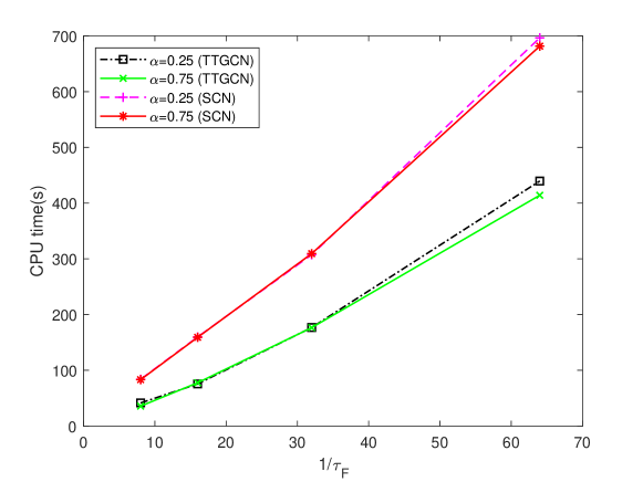
Fig. 1: The comparison of two methods for CPU time with $h=1/100$ and $k=4$ for Example 1.

Fig. 2: The time convergence order with $h=1/100$ and $k=4$ for Example 1.

Example 2

we consider $g(u)=-u-u^{3}$ and $\mu=1$. The exact solution is given via

$$u(x,y,t)=\frac{t^{\alpha+1}}{\Gamma(2+\alpha)}\sin\pi x\sin\pi y,$$

thus, $\psi(x,y)=0$ and the corresponding force term can be obtained as follows

$$\begin{split}f(x,y,t)=&\left(\frac{t^{\alpha}}{\Gamma(\alpha+1)}+\frac{(2\pi^{2}\mu+1)t^{\alpha+1}}{\Gamma(\alpha+2)}+\frac{t^{2\alpha+1}}{\Gamma(2\alpha+2)}\right)\sin\pi x\sin\pi y\\ &+\left(\frac{t^{\alpha+1}}{\Gamma(2+\alpha)}\sin\pi x\sin\pi y\right)^{3}.\end{split}$$

In Table 4, we give the numerical results with $\alpha=0.25$, $0.5$ and $0.75$ calculated using the TTGCN finite difference method and the SCN finite difference method, respectively. This numerical result fully demonstrates that the computational efficiency of the TTGCN finite difference method is much higher than that of the SCN finite difference method. Also, according to the numerical results in Table 5, the order of convergence of the two methods in space $\thickapprox 2$. Therefore, the numerical results are consistent with the theoretical analysis. In addition, we also compared with the method in xu2020time . It is obvious from Table 6 that the TTGCN finite difference method has higher accuracy and convergence order.

When $h=1/100$ and $k=4$, Fig. 3 compares the CPU time of the two-grid finite difference method and the standard finite difference method for the time direction, which intuitively demonstrates the effectiveness of our method. Besides, Fig. 4 shows intuitively temporal second-order convergence of two-grid finite difference method.

Table 4: The $L^{2}$-errors, convergence rates and CPU time (seconds) with $h=1/100$ and $k=4$ for Example 2.

$\alpha$	$\tau_{C}$	$\tau_{F}$	$E_{TTGCN}$	$rate^{t}_{TTGCN}$	$CPU(s)$	$E_{SCN}$	$rate^{t}_{SCN}$	$CPU(s)$
	1/2	1/8	2.9535e-2	*	34.31	2.9535e-2	*	64.26
	1/4	1/16	1.0043e-2	1.5563	71.10	1.0043e-2	1.5563	125.59
0.25	1/8	1/32	3.0208e-3	1.7331	161.96	3.0208e-3	1.7331	264.99
	1/16	1/64	7.9828e-4	1.9200	412.81	7.9828e-4	1.9200	561.79
	1/2	1/8	1.5532e-2	*	32.46	1.5532e-2	*	58.22
	1/4	1/16	4.2840e-3	1.8582	69.57	4.2840e-3	1.8582	120.92
0.5	1/8	1/32	1.0448e-3	2.0357	156.46	1.0448e-3	2.0357	242.71
	1/16	1/64	2.2614e-4	2.2080	391.87	2.2614e-4	2.2080	561.08
	1/2	1/8	7.7945e-3	*	30.86	7.7946e-3	*	59.13
	1/4	1/16	1.7861e-3	2.1256	67.44	1.7861e-3	2.1256	113.23
0.75	1/8	1/32	3.6423e-4	2.2939	156.47	3.6423e-4	2.2939	233.35
	1/16	1/64	6.6431e-5	2.4549	402.73	6.6431e-5	2.4549	545.91

Table 5: The $L^{2}$-errors and convergence rates with $\tau_{C}=1/128$ and $\tau_{F}=1/512$ for Example 2.

$h$	$\alpha=0.2$					$\alpha=0.8$
	$E_{TTGCN}$	$rate^{x}_{TTGCN}$	$E_{SCN}$	$rate^{x}_{SCN}$		$E_{TTGCN}$	$rate^{x}_{TTGCN}$	$E_{SCN}$	$rate^{x}_{SCN}$
1/2	1.8132e-1	*	1.8132e-1	*		1.1940e-1	*	1.1941e-1	*
1/4	4.3294e-2	2.0663	4.3296e-2	2.0663		2.8125e-2	2.0859	2.8133e-2	2.0856
1/8	1.0650e-2	2.0233	1.0652e-2	2.0231		6.9065e-3	2.0259	6.9139e-2	2.0247
1/16	2.6486e-3	2.0070	2.6519e-3	2.0060		1.7133e-3	2.0112	1.7206e-3	2.0066
1/32	6.5992e-4	2.0054	6.6217e-4	2.0017		4.2551e-4	2.0095	4.2932e-4	2.0028

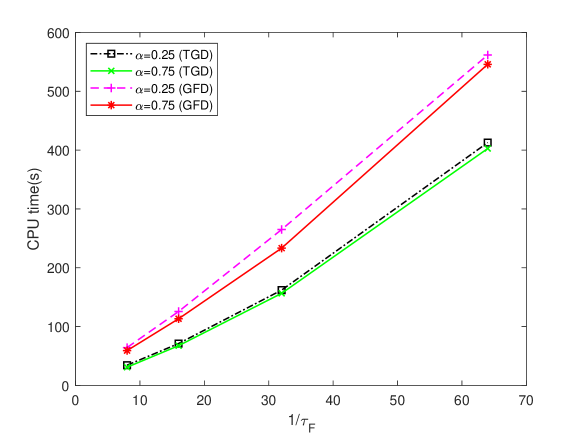
Fig. 3: The CPU time for Example 2 with $h=1/100$ and $k=4$.

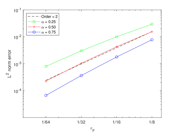
Fig. 4: The time convergence order for Example 2 with $h=1/100$ and $k=4$.

Table 6: The comparison between the scheme (3.9)-(3.13) and the scheme xu2020time whit $h=1/100$ and $k=4$ for Example 2.

$\alpha$	$\tau_{C}$	$\tau_{F}$		Scheme (3.9)-(3.13)			Scheme in xu2020time
				$E_{TTGCN}$	$rate^{t}_{TTGCN}$		$E$	$rate^{t}$
	1/2	1/8		2.9535e-2	*		3.9266e-3	*
	1/4	1/16		1.0043e-2	1.5563		1.9639e-3	0.9996
0.25	1/8	1/32		3.0208e-3	1.7331		9.7001e-4	1.0176
	1/16	1/64		7.9828e-4	1.9200		4.6979e-4	1.0460
	1/2	1/8		1.5532e-2	*		7.6809e-3	*
	1/4	1/16		4.2840e-3	1.8582		3.8683e-3	0.9896
0.5	1/8	1/32		1.0448e-3	2.0357		1.9311e-3	1.0023
	1/16	1/64		2.2614e-4	2.2080		9.5444e-4	1.0167
	1/2	1/8		7.7945e-3	*		9.7620e-3	*
	1/4	1/16		1.7861e-3	2.1256		4.9287e-3	0.9860
0.75	1/8	1/32		3.6423e-4	2.2939		2.2683e-3	0.9977
	1/16	1/64		6.6431e-5	2.4549		1.2266e-3	1.0088

Example 3

we consider

$$u_{t}-\Delta u-I^{(\alpha)}\Delta u=-u^{3},\quad(x,y,t)\in\Omega\times(0,T],$$

$$u(x,y,t)=0,\qquad(x,y)\in\partial\Omega,\quad t\in[0,T],$$

$$u(x,y,0)=xy(1-x)(1-y),\qquad(x,y)\in\Omega.$$

In this example, since the exact solution is unknown, we assume that the numerical solution with fixed spatial step $h=1/32$ and half of the original time steps $\tau_{C}$ and $\tau_{F}$ is the “exact” solution. From Table 7, we can see that for the time direction convergence order TTGCN and SCN finite difference methods in both can approach 2, which agrees with the theoretical analysis.

Table 7: The $L^{2}$-errors and convergence rates with $h=1/32$ and $k=4$ for Example 3

$\alpha$	$\tau_{C}$	$\tau_{F}$	$E_{TTGCN}$	$rate^{t}_{TTGCN}$	$E_{SCN}$	$rate^{t}_{SCN}$
	1/12	1/48	6.0750e-7	*	6.0563e-7	*
	1/24	1/96	1.8258e-7	1.7344	1.8214e-7	1.7334
0.25	1/48	1/192	4.9624e-8	1.8794	4.9558e-8	1.8779
	1/96	1/384	1.2745e-8	1.9611	1.2739e-8	1.9599
	1/12	1/48	1.2281e-6	*	1.2246e-6	*
	1/24	1/96	3.6180e-7	1.7661	3.6036e-7	1.7648
0.5	1/48	1/192	9.7691e-8	1.8860	9.7595e-8	1.8846
	1/96	1/384	2.5272e-8	1.9507	2.5363e-8	1.9498
	1/12	1/48	2.1532e-6	*	2.1477e-6	*
	1/24	1/96	6.3459e-7	1.7626	6.3351e-7	1.7614
0.75	1/48	1/192	1.7308e-7	1.8744	1.7294e-7	1.8731
	1/96	1/384	4.5190e-8	1.9373	4.5177e-8	1.9366

Declaration of Competing Interest

The authors declare that they have no conflict of interest.

References

• [1] Igor Podlubny. Fractional differential equations, academic press, san diego, 1999.
• [2] Leijie Qiao, Wenlin Qiu, and Da Xu. A second-order ADI difference scheme based on non-uniform meshes for the three-dimensional nonlocal evolution problem. Computers & Mathematics with Applications, 102:137–145, 2021.
• [3] Kassem Mustapha and Hussein Mustapha. A second-order accurate numerical method for a semilinear integro-differential equation with a weakly singular kernel. IMA journal of numerical analysis, 30(2):555–578, 2010.
• [4] Avner Friedman and Marvin Shinbrot. Volterra integral equations in banach space. Transactions of the American Mathematical Society, 126(1):131–179, 1967.
• [5] Morton E Gurtin and Allen C Pipkin. A general theory of heat conduction with finite wave speeds. Archive for Rational Mechanics and Analysis, 31(2):113–126, 1968.
• [6] RK Miller. An integrodifferential equation for rigid heat conductors with memory. Journal of Mathematical Analysis and Applications, 66(2):313–332, 1978.
• [7] Hongbin Chen, Da Xu, and Yulong Peng. A second order BDF alternating direction implicit difference scheme for the two-dimensional fractional evolution equation. Applied Mathematical Modelling, 41:54–67, 2017.
• [8] Morrakot Khebchareon, Amiya K Pani, and Graeme Fairweather. Alternating direction implicit Galerkin methods for an evolution equation with a positive-type memory term. Journal of Scientific Computing, 65(3):1166–1188, 2015.
• [9] Chang Ho Kim and U Jin Choi. Spectral collocation methods for a partial integro-differential equation with a weakly singular kernel. The ANZIAM Journal, 39(3):408–430, 1998.
• [10] Stig Larsson, Vidar Thomée, and Lars Wahlbin. Numerical solution of parabolic integro-differential equations by the discontinuous Galerkin method. Mathematics of computation, 67(221):45–71, 1998.
• [11] Limei Li and Da Xu. Alternating direction implicit-Euler method for the two-dimensional fractional evolution equation. Journal of Computational Physics, 236:157–168, 2013.
• [12] Yuan-Ming Wang and Yu-Jia Zhang. A Crank-Nicolson-type compact difference method with the uniform time step for a class of weakly singular parabolic integro-differential equations. Applied Numerical Mathematics, 172:566–590, 2022.
• [13] Mehdi Dehghan and Mostafa Abbaszadeh. Spectral element technique for nonlinear fractional evolution equation, stability and convergence analysis. Applied Numerical Mathematics, 119:51–66, 2017.
• [14] Huifa Jiang, Da Xu, Wenlin Qiu, and Jun Zhou. An ADI compact difference scheme for the two-dimensional semilinear time-fractional mobile–immobile equation. Computational and Applied Mathematics, 39(4):1–17, 2020.
• [15] Ahmed S Hendy, TR Taha, D Suragan, and Mahmoud A Zaky. An energy-preserving computational approach for the semilinear space fractional damped Klein–Gordon equation with a generalized scalar potential. Applied Mathematical Modelling, 108:512–530, 2022.
• [16] Hong-lin Liao, Yonggui Yan, and Jiwei Zhang. Unconditional convergence of a fast two-level linearized algorithm for semilinear subdiffusion equations. Journal of Scientific Computing, 80(1):1–25, 2019.
• [17] Jinchao Xu. Two-grid discretization techniques for linear and nonlinear PDEs. SIAM journal on numerical analysis, 33(5):1759–1777, 1996.
• [18] Jinchao Xu. A novel two-grid method for semilinear elliptic equations. SIAM Journal on Scientific Computing, 15(1):231–237, 1994.
• [19] Clint N Dawson, Mary F Wheeler, and Carol S Woodward. A two-grid finite difference scheme for nonlinear parabolic equations. SIAM journal on numerical analysis, 35(2):435–452, 1998.
• [20] Xiaoli Li and Hongxing Rui. A two-grid block-centered finite difference method for the nonlinear time-fractional parabolic equation. Journal of Scientific Computing, 72(2):863–891, 2017.
• [21] Saumya Bajpai and Neela Nataraj. On a two-grid finite element scheme combined with Crank–Nicolson method for the equations of motion arising in the Kelvin–Voigt model. Computers & Mathematics with Applications, 68(12):2277–2291, 2014.
• [22] Luoping Chen and Yanping Chen. Two-grid method for nonlinear reaction-diffusion equations by mixed finite element methods. Journal of Scientific Computing, 49(3):383–401, 2011.
• [23] Chuanjun Chen and Wei Liu. A two-grid method for finite volume element approximations of second-order nonlinear hyperbolic equations. Journal of Computational and Applied Mathematics, 233(11):2975–2984, 2010.
• [24] Yang Liu, Zudeng Yu, Hong Li, Fawang Liu, and Jinfeng Wang. Time two-mesh algorithm combined with finite element method for time fractional water wave model. International Journal of Heat and Mass Transfer, 120:1132–1145, 2018.
• [25] Da Xu, Jing Guo, and Wenlin Qiu. Time two-grid algorithm based on finite difference method for two-dimensional nonlinear fractional evolution equations. Applied Numerical Mathematics, 152:169–184, 2020.
• [26] William McLean and Kassem Mustapha. A second-order accurate numerical method for a fractional wave equation. Numerische Mathematik, 105(3):481–510, 2007.
• [27] Lj Dedić, M Matić, and J Pečarić. On euler trapezoid formulae. Applied mathematics and computation, 123(1):37–62, 2001.
• [28] Hongbin Chen, Da Xu, and Yulong Peng. An alternating direction implicit fractional trapezoidal rule type difference scheme for the two-dimensional fractional evolution equation. International Journal of Computer Mathematics, 92(10):2178–2197, 2015.
• [29] IH Sloan and V Thomée. Time discretization of an integro-differential equation of parabolic type. SIAM Journal on Numerical Analysis, 23(5):1052–1061, 1986.