Probabilistic Deduction: an Approach to Probabilistic Structured Argumentation

Abstract

This paper introduces Probabilistic Deduction (PD) as an approach to probabilistic structured argumentation. A PD framework is composed of probabilistic rules (p-rules). As rules in classical structured argumentation frameworks, p-rules form deduction systems. In addition, p-rules also represent conditional probabilities that define joint probability distributions. With PD frameworks, one performs probabilistic reasoning by solving Rule-Probabilistic Satisfiability. At the same time, one can obtain an argumentative reading to the probabilistic reasoning with arguments and attacks. In this work, we introduce a probabilistic version of the Closed-World Assumption (P-CWA) and prove that our probabilistic approach coincides with the complete extension in classical argumentation under P-CWA and with maximum entropy reasoning. We present several approaches to compute the joint probability distribution from p-rules for achieving a practical proof theory for PD. PD provides a framework to unify probabilistic reasoning with argumentative reasoning. This is the first work in probabilistic structured argumentation where the joint distribution is not assumed form external sources.

1 Introduction

The field of argumentation has been in rapid development in the past three decades. In argumentation, information forms arguments; one argument attacks another if the former is in conflict with the latter. As stated in Dung’s landmark paper [17], “whether or not a rational agent believes in a statement depends on whether or not the argument supporting this statement can be successfully defended against the counterarguments”, argumentation analyses statement acceptability by studying attack relations amongst arguments. As a reasoning paradigm in multi-agent settings, especially for reasoning under uncertainty or with conflict information, argumentation has seen its applications in e.g. medical (see e.g. [9, 24, 42, 21, 41, 10, 25]), legal (see [5] for an overview), and engineering (see e.g. [60] for an overview) domains.

Arguments in Dung’s abstract argumentation (AA) are atomic without internal structure. Also, in AA, there is no specification of what is an argument or an attack as these notions are assumed to be given. To have a more detailed formalisation of arguments than is available with AA, one turns to structured argumentation - using some forms of logic, arguments are built from a formal language, which serves as a representation of information; attacks are also derived from some notion representing conflicts in the underlying logic and language [3]. Both abstract argumentation and structured argumentation are seen as powerful reasoning paradigms with extensive theoretical results and practical applications (see e.g. [2] for an overview).

As reasoning with probabilistic information is considered a pertinent issue in many application areas, several different probabilistic argumentation frameworks have been developed in the literature to join probability with argumentation. As summarised in Hunter [31], two main approaches to probabilistic argumentation exist today: the epistemic and the constellations approaches. Quoting Hunter & Thimm [37] on this distinction:

In the constellations approach, the uncertainty is in the topology of the graph [of arguments]. …In the epistemic approach, the topology of the argument graph is fixed, but there is uncertainty about whether an argument is believed.

In other words, in a constellations approach, probabilities are defined over sets (extensions) of arguments, representing the uncertainty on whether sets of arguments exist in a given context; whereas in an epistemic approach, probabilities are defined over arguments, representing uncertainty on whether arguments are true. Both approaches have seen many successful development. For instance, [18, 43, 52, 30, 16, 49, 15, 54, 22, 23, 12] are works taking the constellations approach; and [55, 36, 40, 32, 31, 37, 35, 33] are works taking the epistemic approach.

As in non-probabilistic or classical argumentation, arguments in probabilistic argumentation can either be atomic or structured. For instance, amongst the works mentioned above, [18, 23, 52, 31, 32, 33, 12] are the ones studying structured arguments whereas the rest are the ones studying non-structured arguments. Within the group of works that studying probabilistic structured argumentation with the epistemic approach, i.e. [31, 32, 33], it is assumed that a probability distribution over the language is given. An implication of this assumption is that the logic component is detached from the probability component in the sense that one first performs logic operations to form arguments, and then view them through a lens of probability. In other words, there is a “logic information” component describing some knowledge that is used to construct arguments; separately, there is “probability information” which acts as an perspective filter to augment arguments.

Table 1: Examples of Different Probabilistic Argumentation Approaches.

	Abstract	Structured
Constellations	[43, 30, 16, 49, 15, 54, 22, 12]	[18, 52, 23]
Epistemic	[55, 36, 40, 37, 35]	[31, 32, 33]

This work aims to provide an alternative approach to epistemic probabilistic structured argumentation. Instead of assuming the duality of logic and probability, we consider all information being probabilistic and represented in the form of Probabilistic Deduction (PD) frameworks composed of probability rules (p-rules). Being the sole representation in our work, p-rules describe both probability and logic information at the same time as p-rules can be read as both conditional probabilities and production rules. Instead of taking a probability distribution from some external source, p-rules define probability distributions; at the same time, when reading them as production rules, p-rules form a deduction system that can be used to build arguments and attacks as in classical structured argumentation.

Example 1.1.

Consider a hypothetical university admission example with the following information.

• A student is likely to receive good exam scores if he studies hard.
  $\mathtt{GoodExamScore}\leftarrow\mathtt{HardStudy}$:[$0.8$]

• A student is likely to receive good exam scores if he has high IQ.
  $\mathtt{GoodExamScore}\leftarrow\mathtt{HighIQ}$:[$0.6$]

• A student is likely to be admitted to university if he has good exam scores.
  $\mathtt{Admission}\leftarrow\mathtt{GoodExamScore}$:[$0.7$]

• A student is likely not to be admitted if he does not have extracurricular experience.
  $\mathtt{\neg Admission}\leftarrow\mathtt{\neg ExtraExp}$:[$0.7$]

• A student will have extracurricular experience if he has both time and interest for it.
  $\mathtt{ExtraExp}\leftarrow\mathtt{TimeForExtraExp,InterestInExtraExp}$:[$1$]

• A student may or may not have time for extracurricular experience.
  $\mathtt{TimeForExtraExp}\leftarrow$:[$0.5$]

• A student is likely interest in having extracurricular experience.
  $\mathtt{InterestInExtraExp}\leftarrow$:[$0.8$]

• A student may or may not have high IQ.
  $\mathtt{HighIQ}\leftarrow$:[$0.5$]

• A student will not study hard if he is lazy.
  $\neg\mathtt{HardStudy}\leftarrow\mathtt{Lazy}$:[$1$]

Each of these statements is represented with a probabilistic rule (p-rule) denoting conditional probability. For instance,

$\mathtt{GoodExamScore}\leftarrow\mathtt{HardStudy}$:[$0.8$]

is read as

$\Pr(\mathtt{GoodExamScore}|\mathtt{HardStudy})=0.8$;

and

$\mathtt{TimeForExtraExp}\leftarrow$:[$0.5$]

is read as

$\Pr(\mathtt{TimeForExtraExp})=0.5$.

From these p-rules, we can build arguments and specify attacks using the approach we will describe in Section 3. Some arguments and their attacks are shown in Figure 1; and readings of these arguments are summarised in Table 2. With a probability calculation approach we will introduce in Section 2, we compute probabilities for literals as follows:

$\Pr(\mathtt{GoodExamScore})=0.744$,	$\Pr(\mathtt{HardStudy})=0.735$,
$\Pr(\mathtt{HighIQ})=0.5$,	$\Pr(\mathtt{Admission})=0.521$,
$\Pr(\mathtt{ExtraExp})=0.315$,	$\Pr(\mathtt{TimeForExtraExp})=0.5$,
$\Pr(\mathtt{InterestInExtraExp})=0.8$,	$\Pr(\mathtt{Lazy})=0.265$.

With the PD framework we will introduce in Section 3, we compute arguments probabilities as follows.

$\Pr(\mathtt{A})=0.411$,

$\Pr(\mathtt{B})=0.201$,

$\Pr(\mathtt{C})=0.5$,

$\Pr(\mathtt{D})=0.315$.

Figure 1: Some arguments and attacks in Example 1.1. In this example, $\mathtt{HS,GES,Adm,HIQ,EE}$, $\mathtt{TFEE}$, $\mathtt{IIEE}$ are short hands for $\mathtt{HardStudy,GoodExamScore,Admission}$, $\mathtt{HighIQ,ExtraExp}$, $\mathtt{TimeForExtraExp}$, $\mathtt{InterestInExtraExp}$, respectively.

Table 2: Arguments and their readings in Figure 1.

Argument	Reading
$\mathtt{A}$	With hard study, a student will score well in exams.
	Thus they will be admitted to university.
$\mathtt{B}$	With high IQ, a student will score well in exams.
	Thus they will be admitted to university.
$\mathtt{C}$	Without extracurricular experience, a student will not
	be admitted to university.
$\mathtt{D}$	With time and interest, student will have extracurricular experience.

As illustrated in Example 1.1, one can view PD as a representation for probabilistic information supported by a well defined probability semantics. (We will show in Section 2 that the probability semantics is developed from Nilssons’ probabilistic satisfiability (PSAT) [47].) At the same time, there is an argumentative interpretation to PD frameworks in which information can be arranged for presentation with the notions of arguments and attacks. This spirit is inline with contemporary approaches on argumentation for explainable AI (see e.g., [13] for a survey). In these works, there is a “computational layer” for carrying out the computation using any suitable (numerical) techniques, such as machine learning or optimization, and an “argumentation layer” built on top of the “computational layer”, in which the argumentation layer is responsible for producing explanations with argumentation notions such as arguments and attacks. A key property of our work, as we will show in Section 3, is that the two layers reconcile with each other in the sense that when there is no uncertainty with p-rules, i.e. when all p-rules derived from classical argumentation having probability 1, the probability computation coincides with the complete semantics [17] in classical abstract argumentation.

As we intend to let PD frameworks to have practical value, effort has been put into proof theories of PD as we will present in Section 4. In a nutshell, our approach works by viewing each p-rules as a constraint imposed on the probability space defined by the language. We then find a solution in the feasible region as the joint probability distribution. For each literal, we define its probability as the marginal probability computed from the joint probability distribution. For each argument, we define its probability as the sum of probabilities of all models entailing all literals in the argument. The core to our probability computation is finding the joint probability distribution. To this end, we have developed approaches using linear programming, quadratic programming and stochastic gradient descent.

A quick summary of the rest of this paper is as follows.

We introduce the notion of probabilistic rules (p-rules) in Section 2.1, describing its syntax and how p-rules define joint probability distributions. We introduce probability computation of literals in Section 2.2 with two key concepts, probabilistic open-world assumption (P-OWA) and probabilistic closed-world assumption (P-CWA), mimicking their counterparts in non-probabilistic logic. We introduce Maximum Entropy Reasoning in Section 2.3, which give a unique joint probability distribution on each sets of p-rules. As maximum entropy solutions distribute probability “as equally as possible”, we also show an important result (Lemma 2.1) that the probability of a possible world is not zero unless zero is the only value it can take. As both P-CWA and maximum entropy reasoning impose constraints on the joint distribution, we clarify their relations in Section 2.4.

In Section 3, we first give an overview to AA in Section 3.1. We then formally introduce PD framework in Section 3.2, presenting definitions of arguments and attacks in PD frameworks. We connect PD with AA in Section 3.3, showing how AA frameworks can be mapped to PD frameworks in which all p-rules have probability 1. We also present the result that on such mapping, the probability semantics of PD (under P-CWA and Maximum Entropy Reasoning) coincides with the complete extension (Theorem 3.1).

Section 4 presents proof theories of PD frameworks, focusing on the joint probability distribution calculation. Section 4.1 gives the basic approach using linear programming. This is modelled after Nilsson’s PSAT approach [47, 20]. Section 4.2 and 4.3 present approaches for computing joint distributions under P-CWA and with maximum entropy reasoning, respectively. The chief contributions are an algorithm that computes P-CWA “locally” (Theorem 4.2) and using linear entropy in place of von Neumann entropy, respectively. Section 4.4 presents the stochastic gradient descent (SGD) approach for computing joint probabilities. As we show in the performance study in Section 4.5, SGD (with its GPU implementation) is the most practical approach for reasoning with PD frameworks.

This paper builds upon our prior work [20] as follows. The concepts of p-rules and Rule-PSAT (Section 2.1) as well as the linear programming approach for calculating joint probability (Section 4.1) have been presented in [20]. In this paper, we have significantly expanded the theoretical presentation of [20] by introducing the PD framework with a probabilistic version of the closed-world assumption and connecting PD to existing argumentation frameworks. We have also present several scalable techniques for calculating joint probabilities, which pave the way to practical probabilistic structured argumentation.

Proofs of all theoretical results are shown in A.

2 Probabilistic Rules

In this section, we introduce probabilistic rules (p-rules) and satisfiability as the cornerstone of this work. We introduce probabilistic versions of closed-world and open-world assumptions and show how probability of literals can be computed from p-rules with these two assumptions. We introduce the concept of maximum entropy reasoning in the context of p-rules as well.

2.1 Probabilistic Rules and Satisfiability

Given $n$ atoms $\sigma_{0},\ldots,\sigma_{n-1}$ forming a language $\mathcal{L}=\{\sigma_{0},\ldots,\sigma_{n-1}\}$, we let $\mathcal{L}^{c}$ be the closure of $\mathcal{L}$ under the classical negation $\neg$ (namely if $\sigma\in\mathcal{L}$, then $\sigma,\neg\sigma\in\mathcal{L}^{c}$). The core representation of this work, probabilistic rule (p-rule), is defined as follows.

Definition 2.1.

[20] Given a language $\mathcal{L}$, a probabilistic rule (p-rule) is of the form

$$\sigma_{0}\leftarrow\sigma_{1},\ldots,\sigma_{k}:[\theta]$$

for $k\geq 0$, $\sigma_{i}\in\mathcal{L}^{c}$, and $0\leq\theta\leq 1$.

$\sigma_{0}$ is referred to as the head of the p-rule, $\sigma_{1},\ldots,\sigma_{k}$ the body, and $\theta$ the probability.

The p-rule in Definition 2.1 states that the probability of $\sigma_{0}$, when $\sigma_{1}\ldots\sigma_{k}$ all hold, is $\theta$. In other words, this rule states that $\Pr(\sigma_{0}|\sigma_{1},\ldots,\sigma_{k})=\theta$. Without loss of generality, we only consider $\theta>0$ in this work. In other words, for $\sigma_{0}\leftarrow\_:[0]$, one writes $\neg\sigma_{0}\leftarrow\_:[1]$.

Definition 2.2.

[28] Given a language $\mathcal{L}$ with $n$ atoms, the Complete Conjunction Set (CC Set) $\Omega$ of $\mathcal{L}$ is the set of $2^{n}$ conjunction of literals such that each conjunction contains $n$ distinct atoms.

Each $\omega\in\Omega$ is referred to as an atomic conjunction.

$\Omega$ represent the set of all possible worlds and each $\omega\in\Omega$ is one of them. For instance, for $\mathcal{L}=\{\sigma_{0},\sigma_{1}\}$, the CC set of $\mathcal{L}$ is

$$\Omega=\{\neg\sigma_{0}\wedge\neg\sigma_{1},\neg\sigma_{0}\wedge\sigma_{1},\sigma_{0}\wedge\neg\sigma_{1},\sigma_{0}\wedge\sigma_{1}\}.$$

The four atomic conjunctions are: $\neg\sigma_{0}\wedge\neg\sigma_{1},\neg\sigma_{0}\wedge\sigma_{1},\sigma_{0}\wedge\neg\sigma_{1},$ and $\sigma_{0}\wedge\sigma_{1}$.

Definition 2.3.

[20] Given a language $\mathcal{L}$ and a set of p-rules $\mathcal{R}$, let $\Omega$ be the CC set of $\mathcal{L}$. A function $\pi:\Omega\rightarrow[0,1]$ is a consistent probability distribution with respect to $\mathcal{R}$ on $\mathcal{L}$ for $\Omega$ if and only if:

1. For all $\omega_{i}\in\Omega$,

   $$0\leq\pi(\omega_{i})\leq 1;$$ (1)

2. It holds that:

   $$\sum_{\omega_{i}\in\Omega}\pi(\omega_{i})=1.$$ (2)

3. For each p-rule $\sigma_{0}\leftarrow:[\theta]\in\mathcal{R}$, it holds that:

   $$\theta=\sum_{\omega_{i}\in\Omega,\omega_{i}\models\sigma_{0}}\pi(\omega_{i}).$$ (3)

4. For each p-rule $\sigma_{0}\leftarrow\sigma_{1},\ldots,\sigma_{k}:[\theta]\in\mathcal{R}$, $(k>0)$, it holds that:

   $$\theta=\frac{\sum_{\omega_{i}\in\Omega,\omega_{i}\models\sigma_{0}\wedge\ldots\wedge\sigma_{k}}\pi(\omega_{i})}{\sum_{\omega_{i}\in\Omega,\omega_{i}\models\sigma_{1}\wedge\ldots\wedge\sigma_{k}}\pi(\omega_{i})}.$$ (4)

Our notion of consistency as given in Definition 2.3 consists of two parts. Equations 1 and 2 assert $\pi$ being a probability distribution over the CC set of $\mathcal{L}$ with each $\pi(\omega_{i})$ between 0 and 1, and the sum of all $\pi(\omega_{i})$ is 1, respectively. Equations 3 and 4 assert that each p-rule should be viewed as defining conditional probabilities for which the probability of the head of the p-rule conditioned on the body is the probability. When the body is empty, the head is conditioned on the universe. In other words, Equation 3 asserts $\Pr(\sigma_{0})=\theta$, whereas Equation 4 asserts $\Pr(\sigma_{0}|\sigma_{1},\ldots,\sigma_{k})=\theta$.

Example 2.1.

Let $\mathcal{L}=\{\sigma_{0},\sigma_{1}\}$, $\mathcal{R}=\{\sigma_{0}\leftarrow\sigma_{1}:[\alpha];\sigma_{1}\leftarrow:[\beta]\}$. The CC set is $\Omega=\{\neg\sigma_{0}\wedge\neg\sigma_{1},\sigma_{0}\wedge\neg\sigma_{1},\neg\sigma_{0}\wedge\sigma_{1},\sigma_{0}\wedge\sigma_{1}\}$. From $\sigma_{0}\leftarrow\sigma_{1}:[\alpha]$, applying Equation 3, we have

$$\alpha=\frac{\pi(\sigma_{0}\wedge\sigma_{1})}{\pi(\neg\sigma_{0}\wedge\sigma_{1})+\pi(\sigma_{0}\wedge\sigma_{1})}.$$ (5)

From $\sigma_{1}\leftarrow:[\beta]$, applying Equation 4, we have

$$\beta=\pi(\neg\sigma_{0}\wedge\sigma_{1})+\pi(\sigma_{0}\wedge\sigma_{1}).$$ (6)

Applying Equation 2 on $\Omega$, we have

$$\pi(\neg\sigma_{0}\wedge\neg\sigma_{1})+\pi(\sigma_{0}\wedge\neg\sigma_{1})+\pi(\neg\sigma_{0}\wedge\sigma_{1})+\pi(\sigma_{0}\wedge\sigma_{1})=1.$$ (7)

Lastly, check the inequality given in Equation 1,

$$0\leq\pi(\neg\sigma_{0}\wedge\neg\sigma_{1}),\pi(\sigma_{0}\wedge\neg\sigma_{1}),\pi(\neg\sigma_{0}\wedge\sigma_{1}),\pi(\sigma_{0}\wedge\sigma_{1})\leq 1.$$ (8)

$\pi$ is a consistent probability distribution if and only if there is at least one solution to Equations 5-8.

With consistency defined, we are ready to define Rule-PSAT as follows.

Definition 2.4.

[20] The Rule Probabilistic Satisfiability (Rule-PSAT) problem is to determine for a set of p-rules $\mathcal{R}$ on a language $\mathcal{L}$, whether there exists a consistent probability distribution for the CC set of $\mathcal{L}$ with respect to $\mathcal{R}$.

If a consistent probability distribution exists, then $\mathcal{R}$ is Rule-PSAT; otherwise, it is not.

We illustrate Rule-PSAT with Example 2.2.

Example 2.2.

(Example 2.1 continued.) To test whether $\mathcal{R}$ is Rule-PSAT on $\mathcal{L}$, we need to solve Equations 5-8 for $\pi$ as $\mathcal{R}$ is Rule-PSAT if and only if a solution exists. It is easy to see that this is the case as:

$$\pi(\sigma_{0}\wedge\sigma_{1}) =\alpha\beta$$

$$\pi(\neg\sigma_{0}\wedge\sigma_{1}) =\beta-\alpha\beta$$

$$\pi(\sigma_{0}\wedge\neg\sigma_{1})+\pi(\neg\sigma_{0}\wedge\neg\sigma_{1}) =1-\beta$$

Since $0\leq\alpha,\beta\leq 1$, we have $0\leq\pi(\sigma_{0}\wedge\sigma_{1}),\pi(\neg\sigma_{0}\wedge\sigma_{1})\leq 1$. We can let $\pi(\sigma_{0}\wedge\neg\sigma_{1})=0$, $\pi(\neg\sigma_{0}\wedge\neg\sigma_{1})=1-\beta$ and obtain one solution for $\pi$. As the system is underspecified with four unknowns and three equations, we have infinitely many solutions to $\pi(\sigma_{0}\wedge\neg\sigma_{1})$ and $\pi(\neg\sigma_{0}\wedge\neg\sigma_{1})$ in the range of [0, $1-\beta$].

The next example gives a set of p-rules that is not Rule-PSAT.

Example 2.3.

Let $\mathcal{R}$ be a set of three p-rules:

$$\{\sigma_{0}\leftarrow\sigma_{1}:[0.9],\sigma_{0}\leftarrow:[0.8],\sigma_{1}\leftarrow:[0.9]\}.$$

From $\sigma_{0}\leftarrow\sigma_{1}:[0.9]$ and Equation 4, we have

$$0.9=\frac{\pi(\sigma_{0}\wedge\sigma_{1})}{\pi(\sigma_{0}\wedge\sigma_{1})+\pi(\neg\sigma_{0}\wedge\sigma_{1})}.$$ (9)

From $\sigma_{1}\leftarrow:[0.9]$, we have

$$0.9=\pi(\sigma_{0}\wedge\sigma_{1})+\pi(\neg\sigma_{0}\wedge\sigma_{1}).$$ (10)

Subsitute (10) in (9), we have $\pi(\sigma_{0}\wedge\sigma_{1})=0.81$.

From $\sigma_{0}\leftarrow:[0.8]$, we have

$$0.8=\pi(\sigma_{0}\wedge\sigma_{1})+\pi(\sigma_{0}\wedge\neg\sigma_{1}).$$

Thus, $\pi(\sigma_{0}\wedge\neg\sigma_{1})=-0.01$, which does not satisfy $0\leq\pi(\omega_{i})\leq 1$.

Note that there is no restriction imposed on the form of p-rules other than the ones given in Definition 2.1, as illustrated in the next two examples, Examples 2.4 and 2.5, a set of p-rules can be consistent even if there are rules in this set forming cycles or having two rules with the same head.

Example 2.4.

Consider a set of p-rules

$$\{\sigma_{0}\leftarrow\sigma_{1}:[0.7],\sigma_{1}\leftarrow\sigma_{0}:[0.6],\sigma_{1}\leftarrow:[0.5]\}.$$

We can see that there is a cycle between $\sigma_{1}$ and $\sigma_{0}$ as one can deduce $\sigma_{0}$ from $\sigma_{1}$ and deduce $\sigma_{1}$ from $\sigma_{0}$. However, we can still compute a (unique) solution for $\pi$ over the CC set of $\{\sigma_{0},\sigma_{1}\}$. Using Equations 2 to 4, we have:

$$0.7 =\pi(\sigma_{0}\wedge\sigma_{1})/(\pi(\sigma_{0}\wedge\sigma_{1})+\pi(\neg\sigma_{0}\wedge\sigma_{1})),$$

$$0.6 =\pi(\sigma_{0}\wedge\sigma_{1})/(\pi(\sigma_{0}\wedge\sigma_{1})+\pi(\sigma_{0}\wedge\neg\sigma_{1})),$$

$$0.5 =\pi(\sigma_{0}\wedge\sigma_{1})+\pi(\neg\sigma_{0}\wedge\sigma_{1}),$$

$$1 =\pi(\neg\sigma_{0}\wedge\neg\sigma_{1})+\pi(\neg\sigma_{0}\wedge\sigma_{1})+\pi(\sigma_{0}\wedge\neg\sigma_{1})+\pi(\sigma_{0}\wedge\sigma_{1}).$$

A solution is: $\pi(\neg\sigma_{0}\wedge\neg\sigma_{1})=0.27$, $\pi(\sigma_{0}\wedge\neg\sigma_{1})=0.23$, $\pi(\neg\sigma_{0}\wedge\sigma_{1})=0.15$, $\pi(\sigma_{0}\wedge\sigma_{1})=0.35$.

Example 2.5.

Consider a set of p-rules

$$\{\sigma_{0}\leftarrow\sigma_{1}:[0.6],\sigma_{0}\leftarrow\sigma_{2}:[0.5],\sigma_{1}\leftarrow:[0.7],\sigma_{2}\leftarrow:[0.6]\}.$$

There are two p-rules with head $\sigma_{0}$, namely,

$\sigma_{0}\leftarrow\sigma_{1}:[0.6]$ and $\sigma_{0}\leftarrow\sigma_{2}:[0.5]$.

These two p-rules have different bodies and probabilities. We set up equations as follows.

$$0.6 =(\pi(111)+\pi(110))/(\pi(010)+\pi(011)+\pi(110)+\pi(111)),$$

$$0.5 =(\pi(101)+\pi(111))/(\pi(001)+\pi(011)+\pi(101)+\pi(111)),$$

$$0.7 =\pi(010)+\pi(011)+\pi(110)+\pi(111),$$

$$0.6 =\pi(001)+\pi(011)+\pi(101)+\pi(111),$$

$$1 =\pi(000)+\pi(001)+\pi(010)+\pi(011)$$

$$+\pi(100)+\pi(101)+\pi(110)+\pi(111).$$

Solve these, a solution found is follows:

$\pi(000)=0$,	$\pi(001)=0.02$,	$\pi(010)=0$,	$\pi(011)=0.28$,
$\pi(100)=0.15$,	$\pi(101)=0.13$,	$\pi(110)=0.25$,	$\pi(111)=0.17$.

2.2 Probability of Literals

So far, we have defined probability distribution over the CC set of a language. To discuss probabilities of literals in the language, there are two distinct views we can take: probabilistic open-world assumptions (P-OWA) and probabilistic closed-world assumptions (P-CWA), explained as follows.

With P-OWA, from a set of p-rules, we take the stand that:

The probability of a literal is determined by the p-rules deducing the literal in conjunction with some unspecified factors that are not described by all p-rules that are known.

P-CWA is the opposite of the P-OWA, such that:

The probability of a literal is determined by the known p-rules deducing the literal.

P-OWA and P-CWA can be viewed as probabilistic counterparts to Reiter’s classic OWA and CWA [50] in the following way.

• P-OWA and OWA assume that things which cannot be deduced from known information can still be true;

• P-CWA and CWA both assume that the information available is “complete” for reasoning.

We start our discussion with P-OWA. To define literal probability with P-OWA, we need the following result.

Proposition 2.1.

Given a set of p-rules $\mathcal{R}$ over a language $\mathcal{L}$, if there is a consistent probability distribution $\pi$ for $\Omega$ with respect to $\mathcal{R}$, then for any $\sigma\in\mathcal{L}^{c}$, it is the case that:

$$\sum_{\omega_{i}\in\Omega,\omega_{i}\models\sigma}\pi(\omega_{i}) \geq 0,$$ (11)

$$\sum_{\omega_{i}\in\Omega,\omega_{i}\models\sigma}\pi(\omega_{i})+\sum_{\omega_{i}\in\Omega,\omega_{i}\models\neg\sigma}\pi(\omega_{i}) =1.$$ (12)

With Proposition 2.1, we can define probability of literals under P-OWA. Given a set of p-rules $\mathcal{R}$, if there is consistent probability distribution $\pi$ for $\Omega$ with respect to $\mathcal{R}$, then for any $\sigma\in\mathcal{L}^{c}$, the probability of $\sigma$ under P-OWA is $\mathrm{Pr_{o}}(x)$ such that:

$$\mathrm{Pr_{o}}(\sigma)=\sum_{\omega_{i}\in\Omega,\omega_{i}\models\sigma}\pi(\omega_{i}).$$ (13)

Under P-OWA, the literal probability is as defined in [20]. From a Rule-PSAT solution, which characterises a probability distribution over the CC set, one can compute literal probabilities by summing up $\pi(\omega_{i})$. We illustrate literal probability computation in P-OWA in the example below.

Example 2.6.

Consider the set of p-rules

$$\{\sigma_{0}\leftarrow\neg\sigma_{1}:[1],\sigma_{1}\leftarrow:[1]\},$$

which states that $\sigma_{0}$ holds if $\neg\sigma_{1}$ does, and $\sigma_{1}$ holds. With P-OWA, we have the following equations:

$$\pi(\sigma_{0}\wedge\neg\sigma_{1})/(\pi(\sigma_{0}\wedge\neg\sigma_{1})+\pi(\neg\sigma_{0}\wedge\neg\sigma_{1}) =1$$ (14)

$$\pi(\sigma_{0}\wedge\sigma_{1})+\pi(\neg\sigma_{0}\wedge\sigma_{1}) =1$$ (15)

$$\pi(\neg\sigma_{0}\wedge\neg\sigma_{1})+\pi(\neg\sigma_{0}\wedge\sigma_{1})+\pi(\sigma_{0}\wedge\neg\sigma_{1})+\pi(\sigma_{0}\wedge\sigma_{1}) =1$$ (16)

Solve these, a solution to the joint distribution is

$\pi(\neg\sigma_{0}\wedge\neg\sigma_{1})=0$,	$\pi(\neg\sigma_{0}\wedge\sigma_{1})=0.5$,
$\pi(\sigma_{0}\wedge\neg\sigma_{1})=0$,	$\pi(\sigma_{0}\wedge\sigma_{1})=0.5$.

Use Equation 13 to calculate literal probability, we have

$$\mathrm{Pr_{o}}(\sigma_{0}) =\pi(\sigma_{0}\wedge\sigma_{1})+\pi(\sigma_{0}\wedge\neg\sigma_{1})=0.5,$$

$$\mathrm{Pr_{o}}(\sigma_{1}) =\pi(\sigma_{0}\wedge\sigma_{1})+\pi(\neg\sigma_{0}\wedge\sigma_{1})=1.$$

Thus, we read these as:

1. $\sigma_{1}$ holds as we have asserted with the p-rule

   $$\sigma_{1}\leftarrow:[1];$$

2. yet there is a 50/50 chance that $\sigma_{0}$ holds as well, despite that we have the knowledge that $\sigma_{0}$ would hold if $\sigma_{1}$ does not, captured with the p-rule

   $$\sigma_{0}\leftarrow\neg\sigma_{1}:[1].$$

Thus, we see that the world is “open” as $\sigma_{0}$ has a chance to hold, even though we have no way to deduce that with the p-rules we have.

P-CWA asserts more constraints to literal probabilities than P-OWA. With P-CWA, the probability of a literal is determined by all ways of deducing the literal. To define literal probability under P-OWA, we formalize deduction with p-rules using the same notion defined in Assumption-based Argumentation (ABA) [56], as follows.

Definition 2.5.

Given a language $\mathcal{L}$ and a set of p-rules $\mathcal{R}$, a deduction for $\sigma\in\mathcal{L}^{c}$ with $S\subseteq\mathcal{L}^{c}$, denoted $S\vdash_{\mathtt{D}}\sigma$, is a finite tree with nodes labelled by literals in $\mathcal{L}^{c}$ or by $\tau$, the root labelled by $\sigma$, leaves either $\tau$ or literals in $S$, non-leaves $\sigma$, as children, the elements of the body of some rules in $\mathcal{R}$ with head $\sigma$.

With deduction defined, we can define literal probabilities under P-CWA. Formally, let $\{\Sigma_{1}\vdash_{\mathtt{D}}\sigma,\ldots,\Sigma_{m}\vdash_{\mathtt{D}}\sigma\}$ be all maximal deductions for $\sigma$, where $\Sigma_{1}=\{\sigma_{1}^{1},\ldots,\sigma_{k1}^{1}\},\ldots,\Sigma_{m}=\{\sigma_{1}^{m},\ldots,\sigma_{km}^{m}\}$. Let

$$S=\bigwedge\limits_{i=1}^{k1}\sigma_{i}^{1}\vee\ldots\vee\bigwedge\limits_{i=1}^{km}\sigma_{i}^{m}.$$ (17)

Then,

$$\mathrm{Pr_{c}}(\sigma)=\sum_{\omega_{i}\in\Omega,\omega_{i}\models\sigma}\pi(\omega_{i})=\sum_{\omega_{i}\in\Omega,\omega_{i}\models S}\pi(\omega_{i}).$$ (18)

The difference between P-OWA and P-CWA is illustrated in the following example.

Example 2.7.

(Example 2.6 continued.) There are maximal deductions

$\{\neg\sigma_{1},\sigma_{0}\}\vdash_{\mathtt{D}}\sigma_{0}$ and $\{\sigma_{1}\}\vdash_{\mathtt{D}}\sigma_{1}$

for $\sigma_{0}$ and $\sigma_{1}$, respectively. With P-CWA, in addition to Equation 14 - 16, we have an additional constraint derived from $\{\neg\sigma_{1},\sigma_{0}\}\vdash_{\mathtt{D}}\sigma_{0}$:

$$\pi(\sigma_{0}\wedge\sigma_{1})+\pi(\sigma_{0}\wedge\neg\sigma_{1})=\pi(\sigma_{0}\wedge\neg\sigma_{1}).$$ (19)

This is the case as the LHS sums up probabilities on atomic conjunctions that entail $\sigma_{0}$; and the RHS is the atomic conjunction that entails $S=\sigma_{0}\wedge\neg\sigma_{1}$. The (unique) solution to $\pi$ is

$\pi(\neg\sigma_{0}\wedge\neg\sigma_{1})=0$,	$\pi(\neg\sigma_{0}\wedge\sigma_{1})=1$,
$\pi(\sigma_{0}\wedge\neg\sigma_{1})=0$,	$\pi(\sigma_{0}\wedge\sigma_{1})=0$.

With these, we have $\mathrm{Pr_{c}}(\sigma_{0})=0,\mathrm{Pr_{c}}(\sigma_{1})=1$.

Such results match with our intuition:

• With P-CWA, we assume that the only way to obtain $\sigma_{0}$ is by having $\neg\sigma_{1}$ (with the p-rule $\sigma_{0}\leftarrow\neg\sigma_{1}$:[$1$]). However, since we know $\sigma_{1}$ without any doubt (from the p-rule $\sigma_{1}\leftarrow$:[$1$]), there is no room to believe $\neg\sigma_{1}$; thus we cannot not deduce $\sigma_{0}$.

• On the other hand, with P-OWA, we assume that although we can obtain $\sigma_{0}$ from $\neg\sigma_{1}$, but there are other possible ways of deriving $\sigma_{0}$ that we are unaware of, thus not having $\neg\sigma_{1}$ does not suggest that we can rule out a possibility of $\sigma_{0}$.

Another way to look at P-OWA and P-CWA is from Equation 18. Given $\sigma\in\mathcal{L}^{c}$, let $S$ be as defined in Equation 17, then for any $\omega_{i}\in\Omega$, $\omega_{i}\models\sigma$ and $\omega_{i}\not\models S$, it holds that:

$$\pi(\omega_{i})=0.$$ (20)

From Equation 20, as demonstrated in Example 2.7, it is clear that P-CWA imposes additional constraints on the joint distribution $\pi$. Thus, from a set of p-rules that is Rule-PSAT, literal probabilities under P-CWA may be undefined. Consider the following example.

Example 2.8.

Consider the set of p-rules

$$R=\{\sigma_{0}\leftarrow\neg\sigma_{1}:[1],\sigma_{1}\leftarrow:[1],\sigma_{0}\leftarrow:[0.5]\}.$$

Clearly, $R$ is Rule-PSAT with the solution as given in Example 2.6, computed using Equations 14-16. However, if Equation 19 is added to assert P-CWA, then there is no solution to $\pi$. Thus, literal probabilities under P-CWA such as $\mathrm{Pr_{c}}(\sigma_{0})$ and $\mathrm{Pr_{c}}(\sigma_{1})$ are undefined in this example.

We introduce the concept of P-CWA consistency as follows.

Definition 2.6.

A set of p-rules defined with a language $\mathcal{L}$ is P-CWA consistent if and only if it is consistent and for each $\sigma\in\mathcal{L}^{c}$, $0\leq\mathrm{Pr_{c}}(\sigma)\leq 1.$

P-CWA differs from assumptions several standard assumptions made in handling probabilistic systems such as independence (discussed in e.g., [28]) or mutual exclusivity (discussed in e.g., [59]), as illustrated in Example 2.9 below.

Example 2.9.

Consider a p-rule:

$\sigma_{0}\leftarrow\sigma_{1}$:[$\theta$].

By the definition of p-rule, it holds that

$$\Pr(\sigma_{0}|\sigma_{1})=\frac{\Pr(\sigma_{0}\wedge\sigma_{1})}{\Pr(\sigma_{1})}=\theta.$$

• With P-CWA, from the deduction $\{\sigma_{0},\sigma_{1}\}\vdash_{\mathtt{D}}\sigma_{0}$, we have

  $$\Pr(\sigma_{0})=\Pr(\sigma_{0}\wedge\sigma_{1}).$$

  Thus, $\theta=\Pr(\sigma_{0})/\Pr(\sigma_{1})$.

• With the independence assumption, assuming that $\sigma_{0}$ and $\sigma_{1}$ are independent, we have

  $$\Pr(\sigma_{0}\wedge\sigma_{1})=\Pr(\sigma_{0})\Pr(\sigma_{1}).$$

  Thus, $\theta=\Pr(\sigma_{0})$.

• With the mutual exclusivity assumption, assuming that $\sigma_{0}$ and $\sigma_{1}$ are mutually exclusive, we have

  $$\Pr(\sigma_{0}\wedge\sigma_{1})=0.$$

  Thus, $\theta=0$.

It is easy to see that P-CWA also differs from conditional independence [14], which is the main assumption enabling Bayesian network [53], as illustrated in Example 2.10 below.

Example 2.10.

Consider two p-rules:

$\sigma_{0}\leftarrow\sigma_{1}$:[$\theta_{1}$],     $\sigma_{1}\leftarrow\sigma_{2}$:[$\theta_{2}$].

By the definition of p-rule, we have

$$\Pr(\sigma_{0}|\sigma_{1})=\theta_{1},\Pr(\sigma_{1}|\sigma_{2})=\theta_{2}.$$

Use the chain rule,

$$\Pr(\sigma_{0}\wedge\sigma_{1}\wedge\sigma_{2})=\Pr(\sigma_{0}|\sigma_{1}\wedge\sigma_{2})\Pr(\sigma_{1}|\sigma_{2})\Pr(\sigma_{2}).$$

With conditional independence, assuming that $\sigma_{0}$ and $\sigma_{2}$ are conditionally independent given $\sigma_{1}$, we have $\Pr(\sigma_{0}|\sigma_{1}\wedge\sigma_{2})=\Pr(\sigma_{0}|\sigma_{1}).$ Thus,

$$\Pr(\sigma_{0}\wedge\sigma_{1}\wedge\sigma_{2})=\Pr(\sigma_{0}|\sigma_{1})\Pr(\sigma_{1}|\sigma_{2})\Pr(\sigma_{2})=\theta_{1}\theta_{2}\Pr(\sigma_{2}).$$ (21)

With P-CWA, from the deduction $\{\sigma_{1},\sigma_{2}\}\vdash_{\mathtt{D}}\sigma_{1}$ we have

$$\Pr(\sigma_{1})=\Pr(\sigma_{1}\wedge\sigma_{2}).$$

From $\Pr(\sigma_{1}|\sigma_{2})=\theta_{2}$, we have

$$\frac{\Pr(\sigma_{1}\wedge\sigma_{2})}{\Pr(\sigma_{2})}=\theta_{2}.$$

Thus, $\Pr(\sigma_{1})=\theta_{2}\Pr(\sigma_{2})$. From $\Pr(\sigma_{0}|\sigma_{1})=\theta_{1}$, we have

$$\frac{\Pr(\sigma_{0}\wedge\sigma_{1})}{\Pr(\sigma_{1})}=\frac{\Pr(\sigma_{0}\wedge\sigma_{1}\wedge\sigma_{2})+\Pr(\sigma_{0}\wedge\sigma_{1}\wedge\neg\sigma_{2})}{\theta_{2}\Pr(\sigma_{2})}=\theta_{1}.$$

Since $\Pr(\sigma_{1})=\Pr(\sigma_{1}\wedge\sigma_{2})$,

$$\Pr(\sigma_{1}\wedge\neg\sigma_{2})=0.$$

Since $\Pr(\sigma_{0}\wedge\sigma_{1}\wedge\neg\sigma_{2})\leq\Pr(\sigma_{1}\wedge\neg\sigma_{2})$, we have

$$\Pr(\sigma_{0}\wedge\sigma_{1}\wedge\neg\sigma_{2})=0.$$

Therefore, with P-CWA we also obtain

$$\Pr(\sigma_{0}\wedge\sigma_{1}\wedge\sigma_{2})=\theta_{1}\theta_{2}\Pr(\sigma_{2})$$

as with the conditional independence assumption.

However, with P-CWA, from the deduction $\{\sigma_{0},\sigma_{1},\sigma_{2}\}\vdash_{\mathtt{D}}\sigma_{0}$, we also have

$$\Pr(\sigma_{0})=\Pr(\sigma_{0}\wedge\sigma_{1}\wedge\sigma_{2}),$$

which infers that

$$\Pr(\sigma_{0}\wedge\sigma_{1}\wedge\neg\sigma_{2})=\Pr(\sigma_{0}\wedge\neg\sigma_{1}\wedge\sigma_{2})=\Pr(\sigma_{0}\wedge\neg\sigma_{1}\wedge\neg\sigma_{2})=0.$$

These do not hold in general with the conditional independence assumption.

2.3 Maximum Entropy Solutions

As we are solving systems derived from p-rules to compute the joint distribution $\pi$, when the system is underdetermined, multiple solutions exist, as illustrated in the next example.

Example 2.11.

(Example 2.5 continued.) This example shows a system with five equations and eight unknowns. Thus the system is underdetermined. In addition to the solution shown previously, the following is another solution:

$\pi(\omega_{1})=0.14$,	$\pi(\omega_{2})=0.16$,	$\pi(\omega_{3})=0.14$,	$\pi(\omega_{4})=0.14$,
$\pi(\omega_{5})=0$,	$\pi(\omega_{6})=0$,	$\pi(\omega_{7})=0.12$,	$\pi(\omega_{8})=0.3$.

If a set of p-rules $\mathcal{R}$ is satisfiable (or P-CWA consistent), but the solution to $\pi$ is not unique, then the range of the probability of any literal in $\mathcal{L}^{c}$ can be found with optimization. The upper bound of the probability of a literal $\sigma\in\mathcal{L}^{c}$ can be found by maximising $\Pr(\sigma)$ as defined in Equation 13 (with P-OWA) or 18 (with P-CWA), subject to constraints given by the systems derived from the p-rules. The lower bound of $\Pr(\sigma)$ can be found by minimising these equations accordingly.

Example 2.12.

(Example 2.11 continued.) The solution shown in Example 2.5 maximises $\Pr(\sigma_{0})$ ($\Pr(\sigma_{0})=0.7$); whereas the solution in Example 2.11 minimises it $(\Pr(\sigma_{0})=0.42).$

In addition to choosing a solution that maximizes or minimizes the probability of a literal, we can also choose the solution that maximizes the entropy of the joint distribution. The principle of maximum entropy is commonly used in probabilistic reasoning [39, 48], including in probabilistic argumentation as discussed in e.g., [32] and [55]. It states that

amongst the set of distributions that characterize the known information equally well, the distribution with the maximum entropy should be chosen [38].

The entropy of a discrete probability distribution $\{p_{1},p_{2},\ldots\}$ is

$$H(p_{1},p_{2},\ldots)=-\sum_{i}p_{i}\log(p_{i}).$$

In our context, given a language with $n$ atoms, the maximum entropy distribution can be found by maximising

$$H(\pi_{1},\ldots,\pi_{2^{n}})=-\sum_{i=1}^{2^{n}}\pi(\omega_{i})\log(\pi(\omega_{i})),$$ (22)

subject to the system derived from p-rules.

Example 2.13.

(Example 2.12 continued.) The maximum entropy distribution solution found in this example is:

$\pi(\omega_{1})=0.058$,	$\pi(\omega_{2})=0.114$,	$\pi(\omega_{3})=0.094$,	$\pi(\omega_{4})=0.186$,
$\pi(\omega_{5})=0.058$,	$\pi(\omega_{6})=0.07$,	$\pi(\omega_{7})=0.19$,	$\pi(\omega_{8})=0.23$.

With this $\pi$, $\Pr(\sigma_{0})=0.55$.

By the definition of Rule-PSAT and P-CWA consistency, it is easy to see that maximum entropy solution exists and is unique for satisfiable p-rules. Formally,

Proposition 2.2.

Given a set of consistent p-rules, the maximum entropy solution $\pi^{m}$ exists and is uniquely determined.

A maximum entropy solution is as unbiased as possible amongst all solutions [55]. A useful result on maximum entropy solution that we use in Section 3 is the following.

Lemma 2.1.

Given a set of consistent p-rules, for each $\omega\in\Omega$, consider some constant $\alpha_{\omega}$ such that $[0,\alpha_{\omega}]$ is the feasible region for $\pi(\omega)$. Let $\pi^{m}$ be the maximum entropy solution. If $\alpha_{\omega}>0$, then $\pi^{m}(\omega)>0$.

Lemma 2.1 sanctions that a maximum entropy solution asserting a non-zero probability to each $\omega\in\Omega$ if constraints given by p-rules allow such allocation. In other words, with maximum entropy reasoning, $\pi^{m}(\omega)$ is 0 only if there is no other solution $\pi(\omega)$ exists. Consequentially, with maximum entropy solution, literal probabilities are not 0 unless explicitly set by p-rules. Formally,

Corollary 2.1.

Given a set of consistent p-rules, for each $\sigma\in\mathcal{L}$, let $\alpha_{\sigma}\in[0,1]$ be a constant such that $\Pr(\sigma)=\Pr_{x}(\sigma)\leq\alpha_{\sigma}$ (for $x\in\{o,c\}$). With the maximum entropy solution $\pi$, if $\alpha_{\sigma}>0$, then $\Pr(\sigma)>0.$

2.4 Relation between P-CWA and Maximum Entropy Solutions

Although both P-CWA and maximum entropy reasoning restrict the joint probability distribution we can take on the CC set, these are orthogonal concepts. In other words, one can choose to apply either P-CWA, maximum entropy reasoning individually, or both at the same time. They can all lead to different distributions. We illustrate them with the following example.

Example 2.14.

Given a language $\mathcal{L}=\{\sigma_{0},\sigma_{1},\sigma_{2}\}$ and a set of two p-rules:

$\{\sigma_{0}\leftarrow\sigma_{1}:[0.5],\neg\sigma_{1}\leftarrow\sigma_{2}:[0.5]\}$.

With P-OWA, to compute the joint probability distribution on the CC set, we set up three equations over the $2^{3}=8$ unknowns:

$$0.5 =(\pi(110)+\pi(111))/(\pi(010)+\pi(011)+\pi(110)+\pi(111)),$$

$$0.5 =(\pi(001)+\pi(101))/(\pi(001)+\pi(011)+\pi(101)+\pi(111)),$$

$$1 =\pi(000)+\pi(001)+\pi(010)+\pi(011)$$

$$+\pi(100)+\pi(101)+\pi(110)+\pi(111).$$

With P-CWA, we must consider two deductions:

$\{\sigma_{0},\sigma_{1}\}\vdash_{\mathtt{D}}\sigma_{0}$ and $\{\neg\sigma_{1},\sigma_{2}\}\vdash_{\mathtt{D}}\neg\sigma_{1}$.

These assert that:

$$\sum_{\omega\in\Omega,\omega\models\sigma_{0}}\pi(\omega) =\sum_{\omega\in\Omega,\omega\models\sigma_{0}\wedge\sigma_{1}}\pi(\omega),$$

$$\sum_{\omega\in\Omega,\omega\models\neg\sigma_{1}}\pi(\omega) =\sum_{\omega\in\Omega,\omega\models\neg\sigma_{1}\wedge\sigma_{2}}\pi(\omega),$$

which translate to

$$\sum_{\omega\in\Omega,\omega\models\sigma_{0}\wedge\neg\sigma_{1}}\pi(\omega) =\pi(101)+\pi(100)=0,$$

$$\sum_{\omega\in\Omega,\omega\models\neg\sigma_{1}\wedge\neg\sigma_{2}}\pi(\omega) =\pi(000)+\pi(100)=0.$$

The resulting distribution over the CC set is as summarised in Table 3. Note that unlike maximum entropy reasoning, which gives us unique solutions, the two systems used to compute P-OWA and P-CWA without maximum entropy reasoning are underdetermined, so infinitely many solutions exist.

Table 3: P-CWA and Maximum Entropy (ME) Solutions for the P-Rules in Example 2.14.

	$\pi(000)$	$\pi(001)$	$\pi(010)$	$\pi(011)$
P-OWA without ME	1	0	0	0
P-OWA with ME	0.125	0.125	0.125	0.125
P-CWA without ME	0	0.5	0	0.25
P-CWA with ME	0	0.293	0.207	0.146
	$\pi(100)$	$\pi(101)$	$\pi(110)$	$\pi(111)$
P-OWA without ME	0	0	0	0
P-OWA with ME	0.125	0.125	0.125	0.125
P-CWA without ME	0	0	0	0.25
P-CWA with ME	0	0	0.207	0.146

In this section, we have introduced p-rule as the core building block of this work. Its probability semantics is defined with the joint probability distribution over the CC set of the language. We introduce Rule-PSAT to describe consistent p-rule sets. Literal probability is defined as the sum of probabilities of conjunctions that are models of the literal.

We then introduce Probabilistic Open-World and Closed-World assumptions, P-OWA and P-CWA, respectively, modelling their counterparts in non-monotonic logic. We show how literal probability can be computed with respect to both P-OWA and P-CWA. We make a few remarks that P-CWA differs from other common probabilistic assumptions such as independence, mutual exclusivity and conditional independence. We finish this section with an introduction to maximum entropy solutions and show that when the joint distribution is computed with maximum entropy reasoning, literals will not take 0 probability unless that is the only solution they have.

3 Argumentation with P-Rules

Thus far, we have introduced p-rules as the basic building block in probabilistic deduction. In this section, we show how probabilistic arguments can be built with p-rules and how attacks can be defined between arguments. To this end, we formally define Probabilistic Deduction (PD) Framework composed of p-rules. We then show how PD admits Abstract Argumentation [17] as instances.

Note that in this section, we assume p-rules in discussion are Rule-PSAT consistent. Thus there exists a consistent joint probability distribution $\pi$ for the CC set of $\mathcal{L}$. We will discuss several methods for computing joint distributions $\pi$ from a set of p-rules in Section 4. We also assume that P-CWA can be imposed. Thus, unless specified otherwise, we use $\Pr(\_)$ to denote $\mathrm{Pr_{c}}(\_)$ in this section.

3.1 Background: Abstract Argumentation

We briefly review concepts from abstract argumentation (AA).

An Abstract Argumentation (AA) frameworks [17] are pairs $\langle\mathcal{A},\mathcal{T}\rangle$, consisting of a set of abstract arguments, $\mathcal{A}$, and a binary attack relation, $\mathcal{T}$. Given an AA framework $\emph{AF}=\langle\mathcal{A},\mathcal{T}\rangle$, a set of arguments (or extension) $E\subseteq\mathcal{A}$ is

• admissible (in AF) if and only if $\forall\mathtt{A},\mathtt{B}\in E$, $(\mathtt{A},\mathtt{B})\not\in\mathcal{T}$ (i.e. $E$ is conflict-free) and for any $\mathtt{A}\in E$, if $(\mathtt{C},\mathtt{A})\in\mathcal{T}$, then there exists some $\mathtt{B}\in E$ such that $(\mathtt{B},\mathtt{C})\in\mathcal{R}$;

• complete if and only if $E$ is admissible and contains all arguments it defends, where $E$ defends some $\mathtt{A}^{\prime}\in\mathcal{A}$ iff $E$ attacks all arguments that attack $\mathtt{A}^{\prime}$.

Given $\langle\mathcal{A},\mathcal{T}\rangle$ and a set of labels $\Lambda=\{\mathtt{in,out,undec}\}$, a labelling is a total function $\mathcal{A}\mapsto\Lambda$. Given a labelling on some argumentation framework,

• an $\mathtt{in}$-labelled argument is said to be legally $\mathtt{in}$ if and only if all its attackers are labelled $\mathtt{out}$;

• an $\mathtt{out}$-labelled argument is said to be legally $\mathtt{out}$ if and only if it has at least one attacker that is labelled $\mathtt{in}$;

• an $\mathtt{undec}$-labelled argument is said to be legally $\mathtt{undec}$ if and only if not all its attackers are labelled $\mathtt{out}$ and it does not have an attacker that is labelled $\mathtt{in}$.

A complete labelling is a labelling where every $\mathtt{in}$-labelled argument is legally $\mathtt{in}$, every $\mathtt{out}$-labelled argument is legally $\mathtt{out}$ and every $\mathtt{undec}$ labelled argument is legally $\mathtt{undec}$. An important result that connects complete extensions and complete labelling is that arguments that are labelled $\mathtt{in}$ with a complete-labelling belong to a complete extension. [1]

3.2 Probabilistic Deduction Framework

We define Probabilistic Deduction framework as a set of P-CWA consistent p-rules constructed on a language, as follows.

Definition 3.1.

A Probabilistic Deduction (PD) framework is a pair $\langle\mathcal{L},\mathcal{R}\rangle$ where $\mathcal{L}$ is the language, $\mathcal{R}$ is a set of p-rules such that

• for all $\rho\in\mathcal{R}$, literals in $\rho$ are in $\mathcal{L}^{c}$,

• $\mathcal{R}$ is P-CWA consistent.

With a PD framework, we can build arguments as deductions.

Definition 3.2.

Given a PD framework $\langle\mathcal{L},\mathcal{R}\rangle$, an argument for $\sigma\in\mathcal{L}$ supported by $S\subseteq\mathcal{L}$, $R\subseteq\mathcal{R}$, denoted $S\vdash\sigma$ is such that there is a deduction $\mathtt{A}=S\vdash_{\mathtt{D}}\sigma$ in which for each leaf node $N$ in $\mathtt{A}$, either

1. $N$ is labelled by $\tau$, or

2. $N$ is labelled by some $\sigma^{\prime}\in\mathcal{L}$, $\neg\sigma^{\prime}\leftarrow\_:[\cdot]\in\mathcal{R}$ and $|S|>1$.

The condition $|S|>1$ in Definition 3.2 is put in place to remove “negative singleton argument” resulted from p-rules. For instance, consider a PD framework $\langle\mathcal{L},\mathcal{R}\rangle$ with $\mathcal{L}=\{\sigma_{0}\}$, $\mathcal{R}=\{\sigma_{0}\leftarrow:[1]\}.$ Without this condition, we would admit $\{\neg\sigma_{0}\}\vdash_{\mathtt{D}}\neg\sigma_{0}$ as an argument, because

1. $\neg\sigma_{0}\in\mathcal{L}^{c}$ forms a tree by itself in which the root and the leaf are both $\neg\sigma_{0}$,

2. $\neg\neg\sigma_{0}=\sigma_{0}$ and $\sigma_{0}\leftarrow:[1]$ is a p-rule in $\mathcal{R}$.

Intuitively, in this definition of argument, we want to assert that

1. if there is only a single literal $\sigma$ in the deduction, then there must exist a p-rule $\sigma\leftarrow:[\cdot]$ in the set of rules; otherwise,

2. there must be some reason to acknowledge each leaf, either directly through a rule without body, or the existence of some information about the negation of the leaf.

Example 3.1 presents a few deductions for illustration.

Example 3.1.

Consider a language $\mathcal{L}=\{\sigma_{0},\sigma_{1},\sigma_{2},\sigma_{3}\}$ and four sets of p-rules $R_{1},\ldots,R_{4}$, where

• $R_{1}=\{\sigma_{0}\leftarrow:[0.7]\}$,

• $R_{2}=\{\sigma_{1}\leftarrow:[0.8],\sigma_{0}\leftarrow\sigma_{1}:[0.4]\}$,

• $R_{3}=\{\sigma_{1}\leftarrow:[0.7],\neg\sigma_{2}\leftarrow:[0.8],\sigma_{0}\leftarrow\sigma_{1},\neg\sigma_{2}:[0.8]\}$,

• $R_{4}=\{\neg\sigma_{2}\leftarrow\sigma_{3}:[0.7],\sigma_{1}\leftarrow\sigma_{2}:[0.8],\neg\sigma_{0}\leftarrow\sigma_{1}:[0.8]\}$.

Figure 2 shows some examples of arguments built with these sets of p-rules.

Figure 2: Argument examples: $\{\sigma_{0}\}\vdash\sigma_{0}$ (built with $R_{1}$), $\{\sigma_{0},\sigma_{1}\}\vdash\sigma_{0}$ (built with $R_{2}$), $\{\sigma_{0},\sigma_{1},\neg\sigma_{2}\}\vdash\sigma_{0}$ (built with $R_{3}$) and $\{\sigma_{2},\sigma_{1},\neg\sigma_{0}\}\vdash\sigma_{0}$ (built with $R_{4}$) in Example 3.1.

Example 3.2.

(Example 2.14 continued.) With these two p-rules,

$\{\sigma_{0}\leftarrow\sigma_{1}:[0.5],\neg\sigma_{1}\leftarrow\sigma_{2}:[0.5]\}$.

although both $\{\sigma_{0},\sigma_{1}\}\vdash_{\mathtt{D}}\sigma_{0}$ and $\{\neg\sigma_{1},\sigma_{2}\}\vdash_{\mathtt{D}}\neg\sigma_{1}$ are deductions; only $\{\sigma_{0},\sigma_{1}\}\vdash\sigma_{0}$ is a PD argument.

Definition 3.3.

For two arguments $\mathtt{A}=\_\vdash\sigma$ and $\mathtt{B}=\Sigma\vdash\_$ in some PD framework, $\mathtt{A}$ attacks $\mathtt{B}$ if $\neg\sigma\in\Sigma$.

Example 3.3.

Consider a PD framework $\langle\mathcal{L},\mathcal{R}\rangle$ with

$$\mathcal{R}=\{\sigma_{0}\leftarrow:[0.8],\sigma_{1}\leftarrow\neg\sigma_{0}:[0.9]\}.$$

Two arguments $\mathtt{A}=\{\sigma_{0}\}\vdash\sigma_{0}$ and $\mathtt{B}=\{\neg\sigma_{0},\sigma_{1}\}\vdash\sigma_{1}$ can be built with $\mathcal{R}$ such that $\mathtt{A}$ attacks $\mathtt{B}$, as illustrated in Figure 3.

Figure 3: Argument $\mathtt{A}=\{\sigma_{0}\}\vdash\sigma_{0}$ attacks $\mathtt{B}=\{\neg\sigma_{0},\sigma_{1}\}\vdash\sigma_{1}$ in Example 3.3 and 3.8.

At the core of PD semantics is the argument probability, defined as follows.

Definition 3.4.

Given an argument $\mathtt{A}=S\vdash\sigma$, in which $S=\{s_{1},\ldots,s_{k}\}$, the probability of $\mathtt{A}$ is:

$$\Pr(\mathtt{A})=\Pr(s_{i}\wedge\ldots\wedge s_{k})=\sum_{\omega_{i}\in\Omega,\omega_{i}\models s_{1}\wedge\ldots\wedge s_{k}}\pi(\omega_{i}).$$ (23)

Trivially, $0\leq\Pr(\mathtt{A})\leq 1$. We illustrate argument probability in Example 3.4.

Example 3.4.

(Example 3.3 continued.) Consider the following joint distribution computed from the p-rules:

$$\pi(00)=0.02,\pi(01)=0.18,\pi(10)=0.8,\pi(11)=0.$$

Note that the joint distribution is unique. With P-CWA, from $\{\sigma_{1},\neg\sigma_{0}\}\vdash_{\mathtt{D}}\sigma_{1}$, we have

$$\sum_{\omega\in\Omega,\omega\models\sigma_{1}}\pi(\omega)=\sum_{\omega\in\Omega,\omega\models\sigma_{1}\wedge\neg\sigma_{0}}\pi(\omega).$$

This implies $\pi(\sigma_{0}\wedge\sigma_{1})=\pi(11)=0$.

From the joint distribution, we compute literal and argument probabilities using Equations 13 and 23, respectively, as follows.

$$\Pr(\sigma_{0}) =\pi(10)+\pi(11)=0.8,$$

$$\Pr(\neg\sigma_{0}) =\pi(00)+\pi(01)=0.2,$$

$$\Pr(\sigma_{1}) =\pi(01)+\pi(11)=0.18,$$

$$\Pr(\neg\sigma_{1}) =\pi(00)+\pi(10)=0.82,$$

$$\Pr(\{\sigma_{0}\}\vdash\sigma_{0}) =\pi(10)+\pi(11)=0.8,$$

$$\Pr(\{\neg\sigma_{0},\sigma_{1}\}\vdash\sigma_{1}) =\pi(01)=0.18.$$

Probabilities of arguments that forming attack cycles can be computed without any special treatment, as illustrated in the following example.

Example 3.5.

Consider a PD framework with a set of p-rules

$$\{\sigma_{0}\leftarrow\neg\sigma_{1}:[0.9],\sigma_{1}\leftarrow\neg\sigma_{0}:[0.6]\}.$$

Two arguments $\mathtt{A}=\{\neg\sigma_{1},\sigma_{0}\}\vdash\sigma_{0}$ and $\mathtt{B}=\{\neg\sigma_{0},\sigma_{1}\}\vdash\sigma_{1}$ can be built such that $\mathtt{A}$ attacks $\mathtt{B}$ and $\mathtt{B}$ attacks $\mathtt{A}$, as illustrated in Figure 4.

We compute the joint probability distribution as:

$$\pi(00)=0.087,\pi(01)=0.13,\pi(10)=0.783,\pi(11)=0.$$

Note that the joint probability distribution is again unique. With P-CWA, we have

$$\sum_{\omega\in\Omega,\omega\models\sigma_{0}}\pi(\omega)=\sum_{\omega\in\Omega,\omega\models\sigma_{0}\wedge\neg\sigma_{1}}\pi(\omega).$$

and

$$\sum_{\omega\in\Omega,\omega\models\sigma_{1}}\pi(\omega)=\sum_{\omega\in\Omega,\omega\models\sigma_{1}\wedge\neg\sigma_{0}}\pi(\omega).$$

Both imply $\pi(\sigma_{0}\wedge\sigma_{1})=\pi(11)=0$. Thus there are four equations and four unknowns, so the solution is unique.

With these, we compute literal and argument probabilities:

$\Pr(\mathtt{A})=\pi(10)=0.783,$

$\Pr(\mathtt{B})=\pi(01)=0.13.$

Figure 4: Arguments $\mathtt{A}=\{\neg\sigma_{1},\sigma_{0}\}\vdash\sigma_{0}$ and $\mathtt{B}=\{\neg\sigma_{0},\sigma_{1}\}\vdash\sigma_{1}$ attack each other in Example 3.5.

A few observations can be made with our notions of arguments and attacks in PD frameworks as follows.

• Arguments are defined syntactically in that arguments are deductions, which are trees with nodes being literals and edges defined with p-rules.

• Attacks are also defined syntactically, without referring to either literal or argument probabilities, such that argument $\mathtt{A}$ attacks argument $\mathtt{B}$ if and only if the claim of the $\mathtt{A}$ is the negation of some literals in $\mathtt{B}$. In this process, we make no distinction between “undercut” or “rebuttal” as done in some other constructions (see e.g., [19] for some discussion on these concepts).

• The probability semantics of PD framework given in Equation 23 is based on solving the joint distribution $\pi$ over the CC set of the language $\mathcal{L}$ under the P-CWA assumption. Thus, it is by design a “global” semantics in that it requires a sense of “global consistency” as given in Definition 2.6. We give a brief discussion in B.1 about reasoning with PD frameworks that are not P-CWA consistent.

• Given a PD framework, since its joint distribution $\pi$ may not be unique (unless maximum entropy reasoning is enforced), argument probabilities may not be unique, as well (subject to the same maximum entropy reasoning condition). We discuss the calculation of the joint distribution in detail in Section 4.

A few results concerning the argument probability semantics are as follows. Arguments containing both a literal and its negation have 0 probability.

Proposition 3.1.

For any argument $\mathtt{A}=\Sigma\vdash\_$, if $\sigma,\neg\sigma\in\Sigma$, then $\Pr(\mathtt{A})=0$.

Self-attacking arguments have 0 probability.

Proposition 3.2.

For any argument $\mathtt{A}=\Sigma\vdash\sigma$, if $\neg\sigma\in\Sigma$, then $\Pr(\mathtt{A})=0$.

An argument’s probability is no higher than the probability of its claim.

Proposition 3.3.

For any argument $\mathtt{A}=\Sigma\vdash\sigma$, $\Pr(\mathtt{A})\leq\Pr(\sigma)$.

If an argument’s probability equals the probability of its claim, then there is one and only one argument for the claim.

Proposition 3.4.

For any argument $\mathtt{A}=\Sigma\vdash\sigma$, $\Pr(\mathtt{A})=\Pr(\sigma)$ if and only if there is no $\mathtt{B}\neq\mathtt{A}$ such that $\mathtt{B}=\Sigma^{\prime}\vdash\sigma$ and $\Pr(\mathtt{B})\neq 0$.

If an argument is attacked by another argument, then the sum of the probability of the two arguments is no more than 1.

Proposition 3.5.

For any two arguments $\mathtt{A}$ and $\mathtt{B}$, if $\mathtt{A}$ attacks $\mathtt{B}$, then $\Pr(\mathtt{A})+\Pr(\mathtt{B})\leq 1$.

Proposition 3.5 is the first of the two conditions of p-justifiable introduced in [55] (Definition 4), also known as the “coherence criterion” introduced in [36]. Note that the second condition of p-justifiable, the sum of probabilities of an argument and its attackers must be no less than 1 (also known as the “optimistic criterion” in [36]), does not hold in PD in general, as illustrated in the following example.

Example 3.6.

Consider a PD framework with two p-rules

$$\sigma_{0}\leftarrow\neg\sigma_{1}:[0.1],\sigma_{1}\leftarrow:[0.1].$$

Let $\mathtt{A}=\{\sigma_{1}\}\vdash\sigma_{1}$ and $\mathtt{B}=\{\sigma_{0},\neg\sigma_{1}\}\vdash\sigma_{0}$. We compute $\Pr(\mathtt{A})=0.1$ and $\Pr(\mathtt{B})=0.09$. Clearly, $\mathtt{A}$ attacks $\mathtt{B}$, yet $\Pr(\mathtt{A})+\Pr(\mathtt{B})<1$. This example represents a case where a weak argument attacks another weak argument, and the sum of the probabilities of the two is less than 1.

With p-rules, PD naturally support reasoning with both knowledge with uncertainty and “hard” facts in a single framework. A classic example used in defeasible reasoning, “Nixon diamond” introduced by Reiter and Criscuolo [51], can be modelled with a PD framework as shown in Table 4. We can see that both arguments

$\mathtt{A}=\{p,q,n\}\vdash p$ and $\mathtt{B}=\{\neg p,r,n\}\vdash\neg p$

can be drawn such that they attack each other. Calculate their probabilities, we have $\Pr(\mathtt{A})=\Pr(\mathtt{B})=0.5$.

Table 4: Modelling the Nixon diamond example with PD.

Defeasible Knowledge
usually, Quakers are pacifist	$p\leftarrow q$:[$0.5$]
usually, Republicans are not pacifist	$\neg p\leftarrow r$:[$0.5$]
“Hard” Facts
Richard Nixon is a Quaker	$q\leftarrow n$:[$1$]
Richard Nixon is a Republican	$r\leftarrow n$:[$1$]
Nixon exists	$n\leftarrow$:[$1$]

3.3 PD Frameworks and Abstract Argumentation

To show relations between PD and AA [17], we first explore a few classic examples studied with AA to illustrate PD’s probabilistic semantics. We then present a few intermediate results (Proposition 3.6-3.10). With them, we show that PD generalises AA (Theorem 3.1).

We start by presenting a few examples 3.7-3.11. Arguments and attacks shown in these examples are used in [1] to illustrate differences between several classical (non-probabilistic) argumentation semantics. Characteristics of these examples are summarised in Table 5.

Table 5: Example Argumentation Frameworks Characteristics.

Example	Description	Source
Example 3.7	Three arguments and two attacks	Figure 2 in [1]
Example 3.8	Two arguments attack each other	Figure 3 in [1]
Example 3.9	“Floating Acceptance” example	Figure 5 in [1]
Example 3.10	“Cycle of three attacking arguments” example	Figure 6 in [1]
Example 3.11	Stable extension example	Figure 8 in [1]

Example 3.7.

Let $F$ be a PD framework with three p-rules:

$$\{\sigma_{0}\leftarrow:[1],\sigma_{1}\leftarrow\neg\sigma_{0}:[1],\sigma_{2}\leftarrow\neg\sigma_{1}:[1]\}.$$

Let $\mathtt{A}=\{\sigma_{0}\}\vdash\sigma_{0}$, $\mathtt{B}=\{\sigma_{1},\neg\sigma_{0}\}\vdash\sigma_{1}$, $\mathtt{C}=\{\sigma_{2},\neg\sigma_{1}\}\vdash\sigma_{2}$. Arguments and attacks are shown in Figure 5. The joint distribution $\pi$ is such that

$\pi(000)=0$,	$\pi(001)=0$,	$\pi(010)=0$,	$\pi(011)=0$,
$\pi(100)=0$,	$\pi(101)=1$,	$\pi(110)=0$,	$\pi(111)=0$.

With these, we have $\Pr(\mathtt{A})=1$, $\Pr(\mathtt{B})=0$, and $\Pr(\mathtt{C})=1$.

Figure 5: The PD framework shown in Example 3.7

Example 3.8.

Let $F$ be a PD framework with two p-rules:

$$\{\sigma_{0}\leftarrow\neg\sigma_{1}:[1],\sigma_{1}\leftarrow\neg\sigma_{0}:[1]\}.$$

Let $\mathtt{A}=\{\sigma_{0},\neg\sigma_{1}\}\vdash\sigma_{0}$, and $\mathtt{B}=\{\sigma_{1},\neg\sigma_{0}\}\vdash\sigma_{1}$. The arguments and attacks are shown in Figure 3. A joint distribution $\pi$ is such that

$$\pi(00)=0,\pi(01)=0.5,\pi(10)=0.5,\pi(11)=0.$$

With these, we have $\Pr(\mathtt{A})=\Pr(\mathtt{B})=0.5$.

Example 3.9.

Let $F$ be a PD framework with four p-rules:

$\{\sigma_{0}\leftarrow\neg\sigma_{1}:[1]$,

$\sigma_{1}\leftarrow\neg\sigma_{0}:[1]$,

$\sigma_{2}\leftarrow\neg\sigma_{0},\neg\sigma_{1}:[1]$,

$\sigma_{3}\leftarrow\neg\sigma_{2}:[1]\}$.

Let $\mathtt{A}=\{\sigma_{0},\neg\sigma_{1}\}\vdash\sigma_{0}$, $\mathtt{B}=\{\sigma_{1},\neg\sigma_{0}\}\vdash\sigma_{1}$, $\mathtt{C}=\{\sigma_{2},\neg\sigma_{0},\neg\sigma_{1}\}\vdash\sigma_{2}$, and $\mathtt{D}=\{\sigma_{3},\neg\sigma_{2}\}\vdash\sigma_{3}$. The arguments and attacks are shown in Figure 6. The joint distribution $\pi$ is such that

$$\pi(\omega_{i})=\begin{cases}0.5&\quad\text{if }\omega_{i}=\neg\sigma_{0}\wedge\sigma_{1}\wedge\neg\sigma_{2}\wedge\sigma_{3},\\ 0.5&\quad\text{else if }\omega_{i}=\sigma_{0}\wedge\neg\sigma_{1}\wedge\neg\sigma_{2}\wedge\sigma_{3},\\ 0&\quad\text{otherwise.}\end{cases}$$

Compute argument probabilities, we have $\Pr(\mathtt{A})=\Pr(\mathtt{B})=0.5$, $\Pr(\mathtt{C})=0$, and $\Pr(\mathtt{D})=1$.

Figure 6: The 0/1 PD framework shown in Example 3.9.

Example 3.10.

Let $F$ be a PD framework with three p-rules:

$$\{\sigma_{0}\leftarrow\neg\sigma_{1}:[1],\sigma_{1}\leftarrow\neg\sigma_{2}:[1],\sigma_{2}\leftarrow\neg\sigma_{0}:[1]\}.$$

Let $\mathtt{A}=\{\sigma_{0},\neg\sigma_{1}\}\vdash\sigma_{0}$, $\mathtt{B}=\{\sigma_{1},\neg\sigma_{2}\}\vdash\sigma_{1}$, and $\mathtt{C}=\{\sigma_{2},\neg\sigma_{0}\}\vdash\sigma_{2}$. Arguments and attacks are shown in Figure 7. Although $F$ is Rule-PSAT, it is not P-CWA consistent. Thus, there is no consistent joint distribution over the CC set. $\Pr(\mathtt{A})$, $\Pr(\mathtt{B})$ and $\Pr(\mathtt{C})$ are undefined.

Figure 7: The PD framework shown in Example 3.10.

Example 3.11.

Let $F$ be a PD framework with five p-rules:

$\{\sigma_{0}\leftarrow\neg\sigma_{1}:[1],$	$\sigma_{1}\leftarrow\neg\sigma_{0}:[1],$	$\sigma_{2}\leftarrow\neg\sigma_{1},\neg\sigma_{4}:[1],$
$\sigma_{3}\leftarrow\neg\sigma_{2}:[1],$	$\sigma_{4}\leftarrow\neg\sigma_{3}:[1]\}.$

Let $\mathtt{A}=\{\sigma_{0},\neg\sigma_{1}\}\vdash\sigma_{0}$, $\mathtt{B}=\{\sigma_{1},\neg\sigma_{0}\}\vdash\sigma_{1}$, $\mathtt{C}=\{\sigma_{2},\neg\sigma_{1},\neg\sigma_{4}\}\vdash\sigma_{2}$, $\mathtt{D}=\{\sigma_{3},\neg\sigma_{2}\}\vdash\sigma_{3}$, and $\mathtt{E}=\{\sigma_{4},\neg\sigma_{3}\}\vdash\sigma_{4}$. Arguments and attacks are shown in Figure 8. The joint distribution $\pi$ is such that

$$\pi(\omega_{i})=\begin{cases}1&\quad\text{if }\omega_{i}=\neg\sigma_{0}\wedge\sigma_{1}\wedge\neg\sigma_{2}\wedge\sigma_{3}\wedge\neg\sigma_{4},\\ 0&\quad\text{otherwise.}\end{cases}$$

Compute argument probabilities, we have $\Pr(\mathtt{A})=\Pr(\mathtt{C})=\Pr(\mathtt{E})=0$, and $\Pr(\mathtt{B})=\Pr(\mathtt{D})=1$.

Figure 8: The PD framework shown in Example 3.11.

We make two observations from these examples.

• Syntactically, it is straightforward to map AA frameworks to PD frameworks such that a one-to-one mapping between arguments and attacks in an AA frameworks and their counterparts in the mapped PD framework exist. Thus, for any AA framework $F$, there is a counterpart of it represented as a PD framework.

• Semantically, the probability semantics of PD frameworks in these examples behaves intuitively, in the sense that:

  • winning arguments have probability 1;

  • losing arguments have probability 0;

  • arguments that can either win or lose have probability between 0 and 1; and

  • arguments cannot be labelled neither winning nor losing result in inconsistency.

  With these observations, more formally, as we show below, when argument probabilities are viewed as labelling, they represent a complete labelling.

Starting with the syntactical aspect, we define a mapping from AA frameworks to PD frameworks as follows.

Definition 3.5.

The function $\mathtt{AA2PD}$ is a mapping from AA frameworks to PD frameworks such that for an AA framework $\langle\mathcal{A},\mathcal{T}\rangle$, $\mathtt{AA2PD}(\langle\mathcal{A},\mathcal{T}\rangle)=\langle\mathcal{L},\mathcal{R}\rangle$, where:

• $\mathcal{L}=\mathcal{A}$,

• $\mathcal{R}=\{\sigma\leftarrow\neg\sigma_{1},\ldots,\neg\sigma_{m}:[1]|\sigma\in\mathcal{A}$, $\{\sigma_{1},\ldots,\sigma_{m}\}=\{\sigma_{i}|(\sigma_{i},\sigma)\in\mathcal{T}\}\}$.

Proposition 3.6 below sanctions that the arguments and attacks in AA frameworks are mapped to their counterparts in PD frameworks unambiguously.

Proposition 3.6.

Given an AA framework $F=\langle\mathcal{A},\mathcal{T}\rangle$, there exists a function $\mathtt{g}$ that maps arguments in $F$ to arguments in $\mathtt{AA2PD}(F)$ such that for any $(\mathtt{A},\mathtt{B})\in\mathcal{T}$, $\mathtt{g}(\mathtt{A})$ attacks $\mathtt{g}(\mathtt{B})$ in $\mathtt{AA2PD}(F)$.

To establish semantics connections between AA frameworks and PD frameworks, we first introduce AA-PD frameworks as the set of PD frameworks that are mapped from AA frameworks, i.e., let $\mathcal{F}$ be the set of AA frameworks, then the set of AA-PD frameworks is $\{\mathtt{AA2PD}(F)|F\in\mathcal{F}\}$. We observe the following with AA-PD frameworks:

1. unattacked arguments have probability 1 (note that this is the “founded” criterion in [36]), and

2. if an argument $\mathtt{A}$ with probability 1 attacks another argument $\mathtt{B}$, $\mathtt{B}$ will have probability 0.

Formally, we have propositions 3.7 and 3.8 as follows.

Proposition 3.7.

Given an AA-PD framework $F$, for an argument $\mathtt{A}=S\vdash\sigma$ in $F$, if $\mathtt{A}$ is not attacked in $F$, then $\Pr(\mathtt{A})=1$.

Proposition 3.8.

Given an AA-PD framework $F$, for two arguments $\mathtt{A}$ and $\mathtt{B}$ in $F$ such that $\mathtt{A}$ attacks $\mathtt{B}$. If $\Pr(\mathtt{A})=1$ then $\Pr(\mathtt{B})=0$.

Extending Propositions 3.7 and 3.8, we can show that if all attackers of an argument have probability 0, then the argument has probability 1; moreover, if an argument that has been attacked has probability 1, then all of its attackers must have probability 0. Formally,

Proposition 3.9.

Given an AA-PD framework $F$, let $\mathtt{A}$ be an argument in $F$ and $\mathtt{As}$ the set of arguments attacking $\mathtt{A}$, $\mathtt{A}\not\in\mathtt{As}$.

1. If for all $\mathtt{B}\in\mathtt{As}$, $\Pr(\mathtt{B})=0$, then $\Pr(\mathtt{A})=1$.

2. If $\Pr(\mathtt{A})=1$, then for all $\mathtt{B}\in\mathtt{As}$, $\Pr(\mathtt{B})=0$.

An argument has probability 0 if and only if it has an attacker with probability 1.

Proposition 3.10.

Given an AA-PD framework $F$, let $\mathtt{A}$ be an argument in $F$ and $\mathtt{As}$ the set of arguments attacking $\mathtt{A}$, $\mathtt{A}\not\in\mathtt{As}$. With maximum entropy reasoning,

1. if $\Pr(\mathtt{A})=0$, then there exists $\mathtt{B}\in\mathtt{As}$, such that $\Pr(\mathtt{B})=1$;

2. if there exists $\mathtt{B}\in\mathtt{As}$, such that $\Pr(\mathtt{B})=1$, then $\Pr(\mathtt{A})=0$.

Maximum entropy reasoning is a key condition for Proposition 3.10. This proposition does not hold without it, as illustrate in the following example.

Example 3.12.

Consider an AA-PD framework with five p-rules:

$\sigma_{1}\leftarrow\neg\sigma_{2}$:[$1$],	$\sigma_{2}\leftarrow\neg\sigma_{1}$:[$1$],	$\sigma_{3}\leftarrow\neg\sigma_{1},\neg\sigma_{4}$:[$1$],
$\sigma_{4}\leftarrow\neg\sigma_{5}$:[$1$],	$\sigma_{5}\leftarrow\neg\sigma_{4}$:[$1$].

The arguments and attacks are shown in Figure 9. Calculate the joint probability distribution with maximum entropy reasoning, we have the solution

$$\pi(\omega_{i})=\begin{cases}0.25&\quad\text{if }\omega_{i}\in\{01011,01100,10010,10100\},\\ 0&\quad\text{otherwise.}\end{cases}$$

This solution gives $\Pr(\mathtt{A})=\Pr(\mathtt{B})=\Pr(\mathtt{C})=\Pr(\mathtt{D})=0.5$ and $\Pr(\mathtt{E})=0.25$.

Without maximum entropy reasoning, a possible solution is

$$\pi(\omega_{i})=\begin{cases}0.33&\quad\text{if }\omega_{i}\in\{01100,10010,10100\},\\ 0&\quad\text{otherwise.}\end{cases}$$

This joint distribution gives $\Pr(\mathtt{A})=\Pr(\mathtt{C})=0.67,\Pr(\mathtt{B})=\Pr(\mathtt{D})=0.33$ and $\Pr(\mathtt{E})=0.$ Thus, $\Pr(\mathtt{E})=0$ even though neither of the two arguments ($\mathtt{A}$ and $\mathtt{C}$) attacking $\Pr(\mathtt{E})$ has probability 1.

Figure 9: The AA-PD framework shown in Example 3.12.

Propositions 3.7 - 3.10 describe attack relations between PD arguments similar to attacks in AA (or other non-probabilistic argumentation frameworks). For instance, if we consider arguments with probability 0 $\mathtt{out}$ and probability 1 $\mathtt{in}$, then we obtain a labelling-based semantics as shown in [1]. Formally,

Theorem 3.1.

Given an AA PD framework $F$, let $\mathtt{As}$ be the set of arguments in $F$, with maximum entropy reasoning, the Probabilistic Labelling function $\Xi:\mathtt{As}\mapsto\{\mathtt{in},\mathtt{out},\mathtt{undec}\}$ defined as

$$\Xi(\mathtt{A})=\begin{cases}\mathtt{in}&\quad\text{if }\Pr(\mathtt{A})=1,\\ \mathtt{out}&\quad\text{if }\Pr(\mathtt{A})=0,\\ \mathtt{undec}&\quad\text{otherwise.}\end{cases}$$

in which $\mathtt{A}\in\mathtt{As}$, is a complete labelling.

Theorem 3.1 bridges PD and AA semantically as relations between the complete labelling and argument extensions have been studied extensively in e.g., [1, 7, 8]. In short, labelling can be mapped to extensions in the way that given some semantics $s$, arguments that are labelled $\mathtt{in}$ with $s$-labelling belong to an $s$-extension. Moreover, the complete labelling can be viewed at the centre of defining labellings for other semantics [57]. For instance, a grounded labelling is a complete labelling such that the set of arguments labelled in is minimal with respect to set inclusion among all complete labellings; a stable labelling is a complete labelling such that the set of undecided arguments is empty; a preferred labelling is a complete labelling such that the set of arguments labelled in is maximal with respect to set inclusion among all complete labellings [57].

One last result we would like to present on AA-PD framework is the following.

Proposition 3.11.

Given an AA-PD framework $F$, let $\mathtt{A}$ be an argument in $F$ and $\mathtt{As}$ the set of arguments attacking $\mathtt{A}$, $\mathtt{A}\not\in\mathtt{As}$. $\Pr(\mathtt{A})\geq 1-\sum_{\mathtt{B}\in\mathtt{As}}\Pr(\mathtt{B})$.

This is the “optimistic criterion” introduced in [36, 37]. We will discuss more on the relation between AA-PD and probabilistic abstract argumentation in Section 5.1.

In this section, we have introduced arguments built with p-rules and attacks between arguments in PD frameworks. In PD frameworks, arguments are deductions as they are in ABA frameworks, [11]. Attacks are defined syntactically such that an argument $\mathtt{A}$ attacks another argument $\mathtt{B}$ if the claim of $\mathtt{A}$ is the negation of some literal in $\mathtt{B}$. We have compared PD with AA and show that AA can be mapped to PD frameworks containing only rules assigned with probability 1. The key insight is that the probability semantics given by PD can be viewed as a complete labelling as defined in AA.

4 Probability Calculation

So far we have introduced the probability semantics of p-rules in Section 2 and argument construction in Section 3. In both sections, we have assumed that the joint probability distribution $\pi$ for the CC set can be computed. In this section, we study methods for computing $\pi$ from p-rules. We look at methods for computing exact solutions as well as their approximations.

4.1 Compute Joint Distribution with Linear Programming

We begin with methods for computing exact solutions. Given a set of p-rules $\mathcal{R}=\{\rho_{1},\ldots,\rho_{m}\}$ such that $\mathcal{L}$ contains $n$ literals, to test whether $\mathcal{R}$ is Rule-PSAT, we set up a linear system

$$A\pi=B,$$ (24)

where $A$ is an $(m+1)$-by-$2^{n}$ matrix, $\pi=[\pi(\omega_{1}),\ldots,\pi(\omega_{2^{n}})]^{T}$, $B$ an $(m+1)$-by-$1$ matrix. We construct $A$ and $B$ in a way such that $R$ is Rule-PSAT if and only if $\pi$ has a solution in $[0,1]^{2^{n}}$, as follows.

For each rule $\rho_{i}\in\mathcal{R}$, if $\rho_{i}=\sigma_{0}\leftarrow:[\theta]$ has an empty body, then

$$A[i,j]=\begin{cases}1,&\mbox{if }\omega_{j}\models\sigma_{0}\mbox{;}\\ 0,&\mbox{otherwise};\end{cases}$$ (25)

and

$$B[i]=\theta.$$ (26)

Otherwise, $\rho_{i}=\sigma_{0}\leftarrow\sigma_{1},\ldots,\sigma_{k}:[\theta]$, then

$$A[i,j]=\begin{cases}\theta-1,&\mbox{if }\omega_{j}\models\sigma_{0}\wedge\sigma_{1}\wedge\ldots\wedge\sigma_{k}\mbox{;}\\ \theta,&\mbox{if }\omega_{j}\models\neg\sigma_{0}\wedge\sigma_{1}\wedge\ldots\wedge\sigma_{k}\mbox{;}\\ 0,&\mbox{otherwise};\end{cases}$$ (27)

$$B[i]=0.$$ (28)

Row $m+1$ in $A$ and $B$ are $1\ldots 1$ and $1$, respectively.

Example 4.1.

Consider a p-rule set containing two p-rules, $\rho_{0},\rho_{1}$. Let

$$\rho_{0}=\sigma_{0}\leftarrow\sigma_{1}:[\alpha],\rho_{1}=\sigma_{1}\leftarrow:[\beta].$$

Here, $m=2$, $n=2$. From Equations 24 to 28, we have

$$\fixTABwidth{T}A=\bracketMatrixstack{0&\alpha 0\alpha-1\\ 0101\\ 1111},$$

$\pi=[\pi(\neg\sigma_{0}\wedge\neg\sigma_{1}),\pi(\neg\sigma_{0}\wedge\sigma_{1}),\pi(\sigma_{0}\wedge\neg\sigma_{1}),\pi(\sigma_{0}\wedge\sigma_{1})]^{T}$, and $B=[0,\beta,1]^{T}.$ It is easy to see that $\pi$ has solutions as shown in Example 2.2.

Theorem 4.1.

[20] Given a set of p-rules $\mathcal{R}$ on some language $\mathcal{L}$, $\mathcal{R}$ is Rule-PSAT if and only if Equation 24 has a solution for $\pi$ in $[0,1]^{2^{n}}$.

4.2 Compute Joint Distribution under P-CWA

To reason with P-CWA, additional equations must be introduced as constraints. To this end, we revise the construction of matrices $A$ and $B$ in Equation 24 as given in Equations 25 & 27 and Equations 26 & 28, respectively, to meet the requirement given in Equation 18.

In revising constructions of these two matrices, one useful observation we can make is that the P-CWA constraint

$$\sum_{\omega_{i}\in\Omega,\omega_{i}\models x}\pi(\omega_{i})=\sum_{\omega_{i}\in\Omega,\omega_{i}\models S}\pi(\omega_{i})$$

can be computed “locally” in the sense that one does not need to explicitly identify $S$, the disjunction of conjunctions of literals that are in deductions for $x$ (Equation 17), when computing $\Pr(x)$ for each literal $x$. This is important as if we were to identify $S$ explicitly upon computing $\Pr(x)$ for each $x$, then we need to compute all deductions of $x$, which is both repetitive and computationally expensive. We first illustrate the “local computation” idea with two examples and then present the algorithm along with a formal proof.

Consider three p-rules:

$\sigma_{0}\leftarrow\sigma_{1}:[\cdot],\sigma_{1}\leftarrow\sigma_{2}:[\cdot],\sigma_{2}\leftarrow:[\cdot]$.

Directly applying the definition of P-CWA, we have

• $\Pr(\sigma_{0})=\pi(\sigma_{0}\wedge\sigma_{1}\wedge\sigma_{2})$ from the deduction $\{\sigma_{0},\sigma_{1},\sigma_{2}\}\vdash\sigma_{0}$, and

• $\Pr(\sigma_{1})=\pi(\sigma_{1}\wedge\sigma_{2})$ from the deduction $\{\sigma_{1},\sigma_{2}\}\vdash\sigma_{1}$.

However, if we were to take the “global” view and directly encode

$$\Pr(\sigma_{0})=\pi(\sigma_{0}\wedge\sigma_{1}\wedge\sigma_{2})$$

with the equation

$$\sum_{\omega\in\Omega,\omega\models\sigma_{0},\omega\not\models\sigma_{0}\wedge\sigma_{1}\wedge\sigma_{2}}\pi(\omega)=0$$ (29)

then we must traverse all three rules to find the deduction $\{\sigma_{0},\sigma_{1},\sigma_{2}\}\vdash_{\mathtt{D}}\sigma_{0}$. Instead of doing this traversal, we can simply encode

• $\Pr(\sigma_{0})=\pi(\sigma_{0}\wedge\sigma_{1})$ from the p-rule $\sigma_{0}\leftarrow\sigma_{1}:[\cdot]$ with

  $$\sum_{\omega\in\Omega,\omega\models\sigma_{0},\omega\not\models\sigma_{0}\wedge\sigma_{1}}\pi(\omega)=0,$$ (30)

  and

• $\Pr(\sigma_{1})=\pi(\sigma_{1}\wedge\sigma_{2})$ from the p-rule $\sigma_{1}\leftarrow\sigma_{2}:[\cdot]$ with

  $$\sum_{\omega\in\Omega,\omega\models\sigma_{1},\omega\not\models\sigma_{1}\wedge\sigma_{2}}\pi(\omega)=0.$$ (31)

The new equations 30 and 31 are “local” as given a rule $head\leftarrow body$, we simply assert $\Pr(head)=\pi(head\wedge body)$. There is no deduction construction or multi-rule traversal, which is needed for constructing Equation 29. To see their equivalence, we show that they assign the same set of $\omega\in\Omega$ to 0.

Example 4.2.

We examine the $\omega$ assigned to 0 from each equation. To simplify the presentation, we again use the Boolean string representation introduced in Example 2.5 for literals. E.g., “110” denotes $\sigma_{0}\wedge\sigma_{1}\wedge\neg\sigma_{2}$.

• $\Pr(\sigma_{0})=\pi(\sigma_{0}\wedge\sigma_{1}\wedge\sigma_{2})$ asserts that $\pi(100)=\pi(101)=\pi(110)=0$.

• $\Pr(\sigma_{1})=\pi(\sigma_{1}\wedge\sigma_{2})$ asserts that $\pi(010)=\pi(110)=0$.

• $\Pr(\sigma_{0})=\pi(\sigma_{0}\wedge\sigma_{1})$ asserts that $\pi(100)=\pi(101)=0$.

We see that the only difference between

$\Pr(\sigma_{0})=\pi(\sigma_{0}\wedge\sigma_{1}\wedge\sigma_{2})$ and $\Pr(\sigma_{0})=\pi(\sigma_{0}\wedge\sigma_{1})$

is on setting $\pi(110)=0$. Yet, this is asserted by $\Pr(\sigma_{1})=\pi(\sigma_{1}\wedge\sigma_{2})$, which is available in both the “global” and the “local” versions of constraint.

The above example illustrates the case where p-rules with different heads are chained. When there are two p-rules with the same head, e.g., there exist

$\sigma_{0}\leftarrow\sigma_{1}$:[$\cdot$] and $\sigma_{0}\leftarrow\sigma_{2}$:[$\cdot$],

then we assert

$$\Pr(\sigma_{0})=\pi((\sigma_{0}\wedge\sigma_{1})\vee(\sigma_{0}\wedge\sigma_{2}))=\sum_{\omega\in\Omega,\omega\models(\sigma_{0}\wedge\sigma_{1})\vee(\sigma_{0}\wedge\sigma_{2})}\pi(\omega).$$

Example 4.3.

Consider five p-rules:

$\sigma_{0}\leftarrow\sigma_{1}$:[$\cdot$], $\sigma_{0}\leftarrow\sigma_{2}$:[$\cdot$], $\sigma_{1}\leftarrow\sigma_{3}$:[$\cdot$], $\sigma_{2}\leftarrow$:[$\cdot$], $\sigma_{3}\leftarrow$:[$\cdot$].

With a direct application of P-CWA definition, we have

$\Pr(\sigma_{0})=\pi((\sigma_{0}\wedge\sigma_{1}\wedge\sigma_{3})\vee(\sigma_{0}\wedge\sigma_{2}))$ and $\Pr(\sigma_{1})=\pi(\sigma_{1}\wedge\sigma_{3})$.

We show that this is the same as asserting

$\Pr(\sigma_{0})=\pi((\sigma_{0}\wedge\sigma_{1})\vee(\sigma_{0}\wedge\sigma_{2}))$ and $\Pr(\sigma_{1})=\pi(\sigma_{1}\wedge\sigma_{3})$.

Using the Boolean string representation, E.g., “1001” denotes $\sigma_{0}\wedge\neg\sigma_{1}\wedge\neg\sigma_{2}\wedge\sigma_{3}$,

• with $\Pr(\sigma_{0})=\pi((\sigma_{0}\wedge\sigma_{1}\wedge\sigma_{3})\vee(\sigma_{0}\wedge\sigma_{2}))$, we assert

  $$\pi(1000)=\pi(1001)=\pi(1100)=0.$$

• With $\Pr(\sigma_{1})=\pi(\sigma_{1}\wedge\sigma_{3})$, we assert

  $$\pi(0100)=\pi(0110)=\pi(1100)=\pi(1110)=0.$$

• With $\Pr(\sigma_{0})=\pi((\sigma_{0}\wedge\sigma_{1})\vee(\sigma_{0}\wedge\sigma_{2}))$, we assert

  $$\pi(1000)=\pi(1001)=0.$$

We can see that the difference between the “global” constraint

$$\Pr(\sigma_{0})=\pi((\sigma_{0}\wedge\sigma_{1}\wedge\sigma_{3})\vee(\sigma_{0}\wedge\sigma_{2}))$$

and the “local” one

$$\Pr(\sigma_{0})=\pi((\sigma_{0}\wedge\sigma_{1})\vee(\sigma_{0}\wedge\sigma_{2}))$$

is on asserting $\pi(1100)=0$. However, this is asserted by $\Pr(\sigma_{1})=\pi(\sigma_{1}\wedge\sigma_{3})$. Thus the “global” constraint is indeed satisfied by the “local” version.

Summarising these two examples, additional rows of matrices $A$ and $B$ describing P-CWA can be constructed as follows.

Given a set of p-rules $\mathcal{R}$ such that $\Sigma=\{\sigma_{1},\ldots,\sigma_{m}\}$ are heads of p-rules in $\mathcal{R}$, for each $\sigma\in\Sigma$, let

$$\sigma\leftarrow\sigma_{1}^{1},\ldots,\sigma_{l1}^{1}:[\cdot],\ldots,\sigma\leftarrow\sigma_{1}^{m},\ldots,\sigma_{lm}^{m}:[\cdot]$$

be the p-rules in $\mathcal{R}$ with head $\sigma$. We construct

$$s=(\sigma\wedge\sigma_{1}^{1}\wedge\ldots\wedge\sigma_{l1}^{1})\vee\ldots\vee(\sigma\wedge\sigma_{1}^{m}\wedge\ldots\wedge\sigma_{lm}^{m}).$$ (32)

For each $\sigma\in\Sigma$, append a new row $i$ to $A$ such that

$$A[i,j]=\begin{cases}1,&\mbox{if }\omega_{j}\models\sigma\mbox{ and }\omega_{j}\not\models s\mbox{,}\\ 0,&\mbox{otherwise};\end{cases}$$ (33)

and

$$B[i]=0,$$ (34)

where $j=1\ldots 2^{n}$ are the column indices of $A$, $\omega_{j}$ all atomic conjunctions in $\Omega$. Here, we again consider that $\Omega$ is ordered with the Boolean values of its elements as in footnote 7.

Theorem 4.2.

Given a set of p-rules $\mathcal{R}$ on $n$ literals, if there is a solution $\pi\in[0,1]^{2^{n}}$ to

$$A\pi=B$$

with $A$, $B$ constructed with Equations 25, 27, 33 and 26, 28, 34, respectively. Then $\mathcal{R}$ is P-CWA consistent, $\pi$ a P-CWA solution.

Theorem 4.2 sanctions the correctness of coding the P-CWA criterion with local constraints. The proof of this theorem shown in A is long-winded. However, the idea is simple. We first observe that the “global” constraints given by the P-CWA definition, which are defined with respect to deductions, require us setting $\Pr(\omega_{G})=0$ for some $\omega_{G}\in\Omega$; and the “local” constraints, given by Equations 33 and 34, which only need information in the level of p-rules, also set $\Pr(\omega_{L})=0$ for some $\omega_{L}\in\Omega$. This theorem states that $\omega_{G}$s and $\omega_{L}$s are the same set of atomic conjunctions. This is the case as shown by our induction proof that:

1. when each deduction contains a single p-rule, it is obvious to see that the set of $\omega_{L}$s is the same set of $\omega_{G}$s;

2. when a deduction contains multiple p-rules, assume it is the case that $\omega_{L}$s = $\omega_{G}$s, then introducing any a new p-rule will not break the equality. This is the case because for any $\omega$ that is set to $\Pr(\omega)=0$ by the global constraint but not the local constraint defined by the new p-rule, we can find an existing p-rule that sets $\Pr(\omega)=0$ for the same $\omega$.

   To see this, we observe that for a new p-rule of the form

   $$\rho=\sigma_{0}\leftarrow\sigma_{1},\ldots,\sigma_{n}:[\cdot]$$

   with deduction

   $$\mathtt{A}=\{\sigma_{0},\ldots,\sigma_{n},\sigma_{n+1},\ldots,\sigma_{n+m}\}\vdash_{\mathtt{D}}\sigma_{0},$$

   the $\omega$ that is set to $\Pr(\omega)=0$ by $\mathtt{A}$ but not $\rho$ is of the form

   $$\omega=\sigma_{0}\wedge\ldots\wedge\sigma_{n}\wedge\ldots\wedge\neg\sigma_{k}\wedge\ldots$$

   in which $\sigma_{k}\in\{\sigma_{n+1},\ldots,\sigma_{n+m}\}$. However, $\Pr(\omega)=0$ will be set for such $\omega$ by the p-rule

   $$\rho^{\prime}=\sigma^{*}\leftarrow\sigma_{k},\ldots:[\cdot].$$

   $\sigma^{*}$ and $\rho^{\prime}$ must both exist in $\mathtt{A}$ as without them, there would not be $\sigma_{k}\in\mathtt{A}$. With the local constraint, $\rho^{\prime}$ will set $\Pr(\sigma^{*}\wedge\neg\sigma_{k}\wedge\ldots)=0$.

4.3 Compute Maximum Entropy Solutions

To compute the maximum entropy distribution introduced in Section 2.3, we use

Maximize:

$$H(\pi_{1},\ldots,\pi_{2^{n}})=-\sum_{i=1}^{2^{n}}\pi_{i}\log(\pi_{i}),$$ (35)

subject to:

$$A\pi =B,$$

$$0 \leq\pi_{i}.$$

As the objective function $H$ is quadratic, it can no longer be solved with linear programming techniques. Thus, one possibility is to use a quadratic programming (QP) approach, such as a trust-region method [61], which can optimise quadratic objective functions with linear constraints and allow specification of variable bounds.

Alternatively, to maintain linearity hence reducing complexity, instead of maximising the von Neumann entropy $H$ (Equation 36), we can use the linear entropy [6], which approximates $\log(x)$ with $x-1$ (the first term in the Taylor series of $\log(x)$), and maximise

$$H_{l}(\pi_{1},\ldots,\pi_{2^{n}})=-\sum_{i=1}^{2^{n}}\pi_{i}(1-\pi_{i}),$$ (36)

with Lagrange multipliers [4] as follows.

Consider $A$ as a column vector of $m$ row vectors

$$A=\begin{bmatrix}\bm{a_{1}}\\ \vdots\\ \bm{a_{m}}\end{bmatrix},$$

and $B=[b_{1},\ldots,b_{m}]^{T}$. Define an auxiliary function $L$:

$$L(\pi_{1},\ldots,\pi_{2^{n}},\lambda_{1},\ldots,\lambda_{m})=H_{l}(\pi_{1},\ldots,\pi_{2^{n}})-\sum_{i=1}^{m}\lambda_{i}(\bm{a_{i}}\cdot\pi-b_{i}).$$

$\lambda_{1},\ldots,\lambda_{m}$ are the Lagrange multipliers. We need to solve

$$\nabla_{\pi_{1},\ldots,\pi_{2^{n}},\lambda_{1},\ldots,\lambda_{m}}L(\pi_{1},\ldots,\pi_{2^{n}},\lambda_{1},\ldots,\lambda_{m})=0.$$

This amounts to solve the following $m+2^{n}$ equations:

For $i=1\ldots m$:

$$\bm{a_{i}}\cdot\pi-b_{i}=0.$$ (37)

For $j=1\ldots 2^{n}$:

$$\pi_{j}-\sum_{i=1}^{m}\lambda_{i}\bm{a_{i,j}}=0.$$ (38)

Together with the remaining $m$ equations (Equation 37), we have a new system that gives a maximum linear entropy solution to $A\pi=B$.

In a matrix form, we have

$$\fixTABwidth{T}\bracketMatrixstack{A&0\\ I_{2^{n}}-A^{T}}\bracketMatrixstack{\pi\\ \lambda}=\bracketMatrixstack{B\\ 0},$$ (39)

where $I_{2^{n}}$ is the $2^{n}$-by-$2^{n}$ identity matrix, and $\lambda=[\lambda_{1},\ldots,\lambda_{m}]$.

Example 4.4.

Consider a p-rule set with two p-rules

$\sigma_{0}\leftarrow\sigma_{1}:[0.9]$ and $\sigma_{1}\leftarrow:[0.8]$.

To find the maximum linear entropy solution of $\pi$ using Lagrange multipliers, we start by constructing matrices $A$ and $B$ as:

$$\fixTABwidth{T}A=\bracketMatrixstack{0&0.90-0.1\\ 0101\\ 1111},$$

$B=[0,0.8,1]^{T}$. Thus, $m=3$ and

$$\bm{a_{1}}=[0,0.9,0,-0.1],\bm{a_{2}}=[0,1,0,1],\bm{a_{3}}=[1,1,1,1].$$

Using Equations 38 and 37, we have a linear system with 7 equations to solve:

$$0.9\pi_{2}-0.1\pi_{4} =0$$

$$\pi_{2}+\pi_{4} =0.8$$

$$\pi_{1}+\pi_{2}+\pi_{3}+\pi_{4} =1$$

$$\pi_{1}-\lambda_{3} =0$$

$$\pi_{2}-0.9\lambda_{1}-\lambda_{2}-\lambda_{3} =0$$

$$\pi_{3}-\lambda_{3} =0$$

$$\pi_{4}+0.1\lambda_{1}-\lambda_{2}-\lambda_{3} =0$$

In matrix form, we have:

$$\fixTABwidth{T}\bracketMatrixstack{0&0.90-0.1000\\ 0101000\\ 1111000\\ 100000-1\\ 0100-0.9-1-1\\ 001000-1\\ 00010.1-1-1}\bracketMatrixstack{\pi_{1}\\ \pi_{2}\\ \pi_{3}\\ \pi_{4}\\ \lambda_{1}\\ \lambda_{2}\\ \lambda_{3}}=\bracketMatrixstack{0\\ 0.8\\ 1\\ 0\\ 0\\ 0\\ 0}.$$

Solve these, we find:

$\pi_{1}=0.1,$	$\pi_{2}=0.08,$	$\pi_{3}=0.1,$	$\pi_{4}=0.72$,
$\lambda_{1}=-0.64,$	$\lambda_{2}=0.556,$	$\lambda_{3}=0.1.$

Drop auxiliary variables $\lambda_{1}$, $\lambda_{2}$ and $\lambda_{3}$. From $\pi_{1}$ to $\pi_{4}$, we find $\Pr(\sigma_{0})=0.82$, and $\Pr(\sigma_{1})=0.8$.

Figure 10: Linear Entropy vs. von Neumann Entropy Illustration for a language containing a single literal.

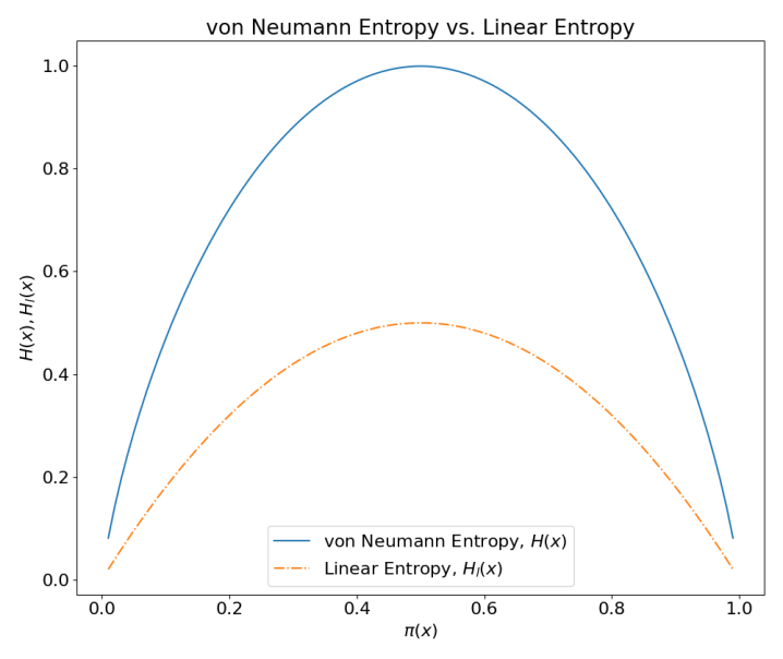
As illustrate in Figure 10, linear entropy, $H_{l}$, gives a lower bound to von Neumann entropy $H$. More importantly, both $H$ and $H_{l}$ attain their maxima when the probabilities are most equally distributed. It is easy to see that the distribution that maximize linear entropy also maximizes von Neumann entropy; thus we do not lose accuracy while maximizing linear entropy.

4.4 Compute Solutions with Stochastic Gradient Descent

So far, all discussions on calculating the joint distribution is centered on solving the linear system

$$A\pi=B$$

with different constructions of $A$ and $B$. Although linear programming with linprog computes solutions, it is computationally expensive. To have a more efficient approach, we consider a stochastic gradient descent (SGD) method for solving $A\pi=B$ as follows.

Let $A=[\bm{a_{1}},\ldots,\bm{a_{m}}]^{T}$, for $i=1,\ldots,m$, define

$$h_{\pi}(\bm{a}_{i})=\bm{a}_{i}\cdot\pi.$$

Consider the squared loss function $L$:

$$L(h_{\pi}(\bm{a}_{i}))=\sum^{m}_{i=1}(\bm{a}_{i}\cdot\pi-b_{i})^{2}.$$

Then, solve $A\pi=B$ is to find $\pi^{*}$, such that

$$\pi^{*} =\operatorname*{arg\,min}_{\pi}\sum_{i=1}^{m}L(h_{\pi}(\bm{a}_{i}))$$

$$=\operatorname*{arg\,min}_{\pi}\sum^{m}_{i=1}(\bm{a}_{i}\cdot\pi-b_{i})^{2}.$$

Use SGD to find the minimum point. For some initial $\pi=[\pi_{1},\ldots,\pi_{2^{n}}]$, loop $i$ in $1,\ldots,m$, each $\pi_{j}$ in $\pi$ is updated iteratively with

$$\pi_{j}\Leftarrow\min(1,\max(0,\pi_{j}+\Delta\pi_{j}))$$ (40)

in which

$$\Delta\pi_{j} =\eta\times\frac{\partial}{\partial\pi_{j}}(\bm{a}_{i}\cdot\pi-b_{i})^{2}$$

$$=\eta\times 2(\bm{a}_{i}\cdot\pi-b_{i})\frac{\partial}{\partial\pi_{j}}(\bm{a}_{i}\cdot\pi-b_{i})$$

$$=\eta\times 2(\bm{a}_{i}\cdot\pi-b_{i})\bm{a}_{ij},$$

where $\eta$ is the learning rate (a small positive number).

Such a root finding process can be viewed as training an unthresholded perceptron model [53] without activation function using SGD. Each $\pi_{i}$ is bounded in $[0,1]$ in the updating step (Equation 40). Note that this is a generic method for solving linear systems. It does not rely on any specific construction of $A$ or $B$. Thus, to compute maximum entropy solutions, we can use this approach to solve the linear system composed of Equation 37 and 38.

A prominent advantage of SGD based approach is the ability to control the error $\zeta=A\pi-B$ at run time, so the gradient descent loop terminates when $|\zeta|$ is “small enough”. Moreover, as SGD can be easily parallelized on GPU, its performance can be improved significantly.

4.5 Computational Performance Studies

To study the performance of presented Rule-PSAT algorithms, we experiment them on randomly generated p-rules. Given a language $\mathcal{L}$, to ensure that p-rule sets defined over $\mathcal{L}$ are Rule-PSAT, we first generate a random distribution $\pi$ over the CC set of $\mathcal{L}$ by drawing samples from a discrete uniform distribution. Then we generate p-rules by randomly selecting literals from $\mathcal{L}$ to be the head and body of p-rules. The length of each p-rule is randomly selected between 1 and the size of the language. The probability of each generated p-rule is then computed from $\pi$ with Equations 3 and 4.

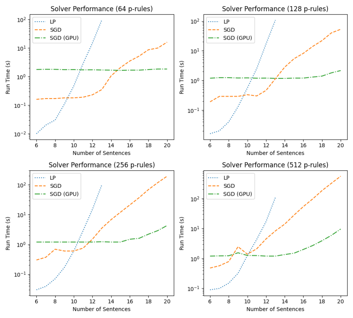
We separate our experiments into two groups, approaches that find a solution to $A\pi=B$ and approaches that find maximum entropy solutions. Figure 11 shows the solver performances for the first gruop: LP, SGD (CPU) and SGD (GPU). In these experiments, the size of the language ranges from $n=6$ to $n=20$; the lengths of p-rule sets are 64, 128, 256 and 512, respectively. The termination condition for SGD (with and without GPU) is $|\zeta|<10^{-3}$. All experiments are conducted on a desktop PC with a Ryzen 2700 CPU (16 cores), 64GB RAM and a Nvidia 3090 GPU (24GB RAM). From this figure, we observe that although LP is faster than SGD when the size of the language is smaller than 10, SGD is significantly faster as the size of $\mathcal{L}$ grows, especially when the GPU implementation is used.

Figure 11: Solver Performance for algorithms that find a solution to $A\pi=B$.

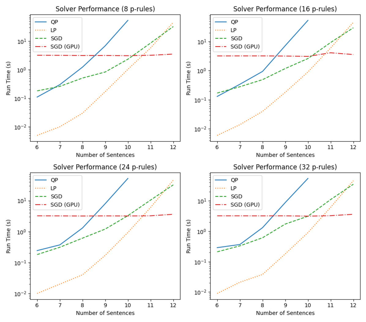
To study performances of approaches that compute maximum entropy solutions, we first compare the entropy of solutions found by these approaches with results shown in Table 6. We observe that approaches that optimize for linear entropy find the same solutions as the QP approach that maximizes von Neumann entropy, as expected. The small differences between these methods are likely caused by numerical errors. For these experiments, the size of p-rule sets is 16. Figure 12 presents the solver performance in terms of speed. We see that although SGD is slower than LP and QP initially, it over takes LP and QP as the size of the $\mathcal{L}$ grows.

Table 6: Entropies of Solutions found by different Approaches with Languages of difference Sizes.

Method	$|\mathcal{L}|$ = 6	$|\mathcal{L}|$ = 7	$|\mathcal{L}|$ = 8	$|\mathcal{L}|$ = 9	$|\mathcal{L}|$ = 10
QP maximize $-\sum\pi_{i}\log(\pi_{i})$	4.101	4.820	5.529	6.235	6.928
LP maximize $-\sum\pi_{i}(\pi_{i}-1)$	4.103	4.821	5.529	6.235	6.928
SGD maximize $-\sum\pi_{i}(\pi_{i}-1)$	4.101	4.824	5.529	6.235	6.929

Figure 12: Solver Performance for algorithms that find maximum entropy solution to $A\pi=B$.

In all experiments, the learning rate $\eta$ in our SGD implementations are set to $1/2^{n}$, where $n$ is the size of the language. A common technique, momentum [45], in training neural networks have been applied to speed up the SGD convergence rate. Namely, in each iteration, $\Delta\pi_{j}$ is updated with

$$\Delta\pi_{j}\Leftarrow\eta\times 2(\bm{a}_{i}\cdot\pi-b_{i})\bm{a}_{ij}+\alpha\Delta\pi_{j},$$

where $\alpha=0.99$ is the momentum used in all experiments. $\Delta\pi_{j}$ on the RHS is $\Delta\pi_{j}$ calculated in the previous iteration.

In summary, Table 7 presents characteristics of the Rule-PSAT solving approaches studied in this work. We see that SGD approaches with GPU implementation significantly outperform LP and QP methods in terms of scalability.

Table 7: Characteristics of Rule-PSAT Solving Approaches introduced in this section.

	Exact	Maximum
Method	Solution	Entropy Solution
LP solve $A\pi=B$	Yes	No
QP maximize $-\sum\pi_{i}\log(\pi_{i})$	Yes	Yes (von Neumann)
LP maximize $-\sum\pi_{i}(\pi_{i}-1)$	Yes	Yes (Linear)
SGD solve $A\pi=B$	No	No
SGD maximize $-\sum\pi_{i}(\pi_{i}-1)$	No	Yes (Linear)
SGD solve $A\pi=B$ (GPU)	No	No
SGD maximize $-\sum\pi_{i}(\pi_{i}-1)$ (GPU)	No	Yes (Linear)

5 Discussion and Conclusion

In this work, we have presented a novel probabilistic structured argumentation framework, Probabilistic Deduction (PD). Syntactically, PD frameworks are defined with probabilistic rules (p-rules) in the form of

$$\sigma_{0}\leftarrow\sigma_{1},\ldots,\sigma_{n}:[\theta],$$

which is read as conditional probabilities $\Pr(\sigma_{0}|\sigma_{1},\ldots,\sigma_{n})=\theta$. To reason with p-rules, we solve the rule probabilistic satisfiability problem to find the joint probability distribution over the language defining the p-rules and then compute literal probabilities for literals in the language. We have introduced two different formulations for this process, the probabilistic open-world assumption (P-OWA) and probabilistic closed-world assumption (P-CWA). With P-OWA, the joint probability is solved based on conditional probabilities defined by p-rules; with P-CWA, additional constraints are introduced to assert that the probability of a literal is the sum of all possible worlds that contain a deduction to the literal.

From p-rules, we build arguments as deductions in the way that the leaves of a deduction are either literals that are heads of p-rules with empty bodies or literals for which there are p-rules for their negations. One argument attacks another when the claim of the former is the negation of some literal in the latter. The main technical achievement in this part is that we prove that with maximum entropy reasoning, our probability semantics with P-CWA coincide with the complete semantics defined for non-probabilistic argumentation. We prove this abstract argumentation with mappings from AA frameworks to PD presented.

Solving Rule-PSAT is at the core of reasoning with PD. We have investigated several different approaches for doing this using linear programming, quadratic programming and stochastic gradient descent. We have conducted experiments with these approaches on p-rule sets built on different sizes of languages and with different numbers of p-rules. We observe that stochastic gradient descent with GPU implementation outperforms all other approaches as the size of the language grows.

5.1 Relations with some Existing Works

As discussed in [20], Rule-PSAT is a variation of the probabilistic satisfiability (PSAT) problem introduced by Nilsson in [47]. Nilsson considered knowledge bases in Conjunctive Normal Form. A modus ponens example,

If $\sigma_{1}$, then $\sigma_{0}$. $\sigma_{1}$. Therefore, $\sigma_{0}$.

is shown in Table 8. The probabilities of the conditional claim is $\alpha$, the antecedent $\beta$ and the consequent $\gamma$. With Nilsson’s probabilistic logic, this is interpreated as:

$\neg\sigma_{1}\vee\sigma_{0}:[\alpha]$,

$\sigma_{1}:[\beta]$,

$\sigma_{0}:[\gamma]$,

which gives rise to equations

$$\pi(\neg\sigma_{1}\wedge\sigma_{0})+\pi(\sigma_{1}\wedge\sigma_{0})+\pi(\neg\sigma_{1}\wedge\neg\sigma_{0}) =\alpha,$$ (41)

$$\pi(\sigma_{1}\wedge\sigma_{0})+\pi(\sigma_{1}\wedge\neg\sigma_{0}) =\beta,$$ (42)

$$\pi(\sigma_{1}\wedge\sigma_{0})+\pi(\neg\sigma_{1}\wedge\sigma_{0}) =\gamma.$$ (43)

With probabilistic rules discussed in this work, the interpreatation to modus ponens is the three p-rules as follows.

$\sigma_{0}\leftarrow\sigma_{1}:[\alpha]$,

$\sigma_{1}\leftarrow:[\beta]$,

$\sigma_{0}\leftarrow:[\gamma]$,

which gives rise to equations

$$\frac{\pi(\sigma_{0}\wedge\sigma_{1})}{\pi(\neg\sigma_{0}\wedge\sigma_{1})+\pi(\sigma_{0}\wedge\sigma_{1})} =\alpha,$$ (44)

42 and 43. The two shaded polyhedrons shown in Table 8 illustrate probabilistic consistent regions for $\alpha,\beta$ and $\gamma$, with probabilistic logic and probabilistic rule, respectively, as defined by their corresponding equations together with equations 1 and 2. The consistent region in the probabilistic logic case is a tetrahedron, with vertices (0,0,1), (1,0,0), (1,1,0) and (1,1,1). The consistent region in the probabilistic rule case is an octahedron, with vertices (0,0,0), (0,0,1), (0,1,0), (1,0,0), (1,1,0) and (1,1,1). It is argued in [46] that the conditional probability interpretation to modus ponens is more reasonable than the probabilistic logic interpretation in practical settings.

Table 8: Comparison of Consistent Probability Regions between Nilsson’s Probabilistic Logic and Probabilistic Rules on an modus ponens instance. [20]

Probabilistic Logic	Probabilistic Rule
$\neg\sigma_{1}\vee\sigma_{0}:[\alpha]$,     $\sigma_{1}:[\beta]$,     $\sigma_{0}:[\gamma]$.	$\sigma_{0}\leftarrow\sigma_{1}:[\alpha]$, $\sigma_{1}\leftarrow:[\beta]$, $\sigma_{0}\leftarrow:[\gamma]$.

From this example, we observe that both methods are nothing but imposing constraints on the feasible regions of the spaces defined by clauses (in the case of probabilistic logic) or p-rules (in the case of probabilistic rules). In this sense, reasoning on such probability and logic combined forms is about identifying feasible regions determined by solutions to $\Pi$ in $A\Pi=B$.

Hunter and Liu [34] make an interesting observation on representing scientific knowledge by combining probabilistic reasoning with logical reasoning. Quoting from [34]:

A key shortcoming of extending classical logic in order to handle probabilistic or statistical information, either by using a possible worlds approach or by adding a probability distribution to each model, is the computational complexity that it involves.

They suggest one may circumvent the computation of joint probability distribution by considering approaches such as Bayesian networks. We certainly agree that computational difficulty is a major challenge. On the other hand, as [26] have shown that the problem of PSAT is NP-complete, thus there does not exist a shortcut that performs probabilistic reasoning “correctly” in general cases. Thus, any probabilistic reasoning approach that does not require the computation of the joint probabilistic distribution either imposes probabilistic assumptions in the underlying model such as independence e.g., [44, 28], or topological constraints, e.g., conditional independence [14], as in Bayesian networks. In this work, we choose not to make such assumptions and study computational approaches with optimization techniques.

In the landscape of probabilistic argumentation, [55, 36, 37] give detailed account on probabilistic abstract argumentation with the epistemic approach. They have described some “desirable” properties of probability semantics, which can be viewed as properties imposed on the joint probability distribution. As discussed in Section 1, the main difference distinguishes this work with existing ones is that we do not assume a given joint probability distribution. Yet, with our approach, we can still compute argument probabilities and thus compare with some of the properties they have proposed, as follows.

• COH A probability distribution $P$ is coherent if for arguments $\mathtt{A}$ and $\mathtt{B}$, if $\mathtt{A}$ attacks $\mathtt{B}$, then $\Pr(\mathtt{A})+\Pr(\mathtt{B})\leq 1$.

  As shown in Proposition 3.5, COH holds in PD frameworks in general.

• SFOU $P$ is semi-founded if $\Pr(\mathtt{A})\geq 0.5$ for every $\mathtt{A}$ not attacked.

  This is not true in general PD frameworks, as one can use a p-rule

  $$\sigma_{0}\leftarrow:[0.2],$$

  to build an un-attacked argument $\mathtt{A}=\{\sigma_{0}\}\vdash\sigma_{0}$, $\Pr(\mathtt{A})=0.2\leq 0.5$. However, SFOU holds for AA-PD frameworks, as shown by Proposition 3.7.

• FOU $P$ is founded if all un-attacked argument have probability 1.

  This is not true in general PD frameworks, but true for AA-PD frameworks, as shown by Proposition 3.7.

• SOPT $P$ is semi-optimistic if $\Pr(\mathtt{A})\geq 1-\sum_{\mathtt{B}\in\mathtt{Bs}}\Pr(\mathtt{B})$, where $\mathtt{Bs}\neq\{\}$ is the set of arguments attacking $\mathtt{A}$.

  This is not true in general PD frameworks, as demonstrated in Example 3.6. This is true for AA-PD framework as shown by Proposition 3.11.

• OPT $P$ is optimistic if $\Pr(\mathtt{A})\geq 1-\sum_{\mathtt{B}\in\mathtt{Bs}}\Pr(\mathtt{B})$, where $\mathtt{Bs}$ is the set of arguments attacking $\mathtt{A}$.

  As in the previous case, this is not true in general PD framework but true for AA-PD frameworks by Proposition 3.11.

• JUS $P$ is justifiable if $P$ is coherent and optimistic.

  Since PD frameworks are not optimistic in general, they are not justifiable. AA-PD frameworks are justifiable.

• TER $P$ is ternary if $\Pr(\mathtt{A})\in\{0,0.5,1\}$ for all $\mathtt{A}$.

  This is not true in general PD frameworks as shown in e.g., Example 1.1. This is not true for AA-PD framework either, as illustrated in Example 3.12.

This comparison is encouraging as one can take these properties introduced by Hunter and Thimm as a benchmark for probabilistic argumentation semantics. Observing AA-PD frameworks, a subset of PD frameworks, confirm to these properties helps us to see the underlying connection between PD frameworks and existing works on probabilistic argumentation. At the same, since general PD frameworks do not confirm to the founded and optimistic properties, we observe the hierarchical structure as shown in Figure 13.

Figure 13: The hierarchical structure between p-rules, PD frameworks and AA-PD frameworks.

PD frameworks share some similarities with Probabilistic Assumption-based Argumentation (PABA) [18, 29, 12], syntactically. [20] has presented differences between p-rules and PABA. Namely, PABA disallows rules forming cycles and if two rules have the same head, the body of one must be a subset of the other; whereas p-rules do not have these constraints. PD frameworks and AA-PD frameworks introduced in this work do not have these constraints. More fundamentally, PABA is an constellation approach to probabilistic argumentation [12], whereas PD is an epistemic approach.

5.2 Future Work

Moving forward, there are three main research directions we will explore in the future. Firstly, as briefly explained in Section B.1, the current approaches for computing literal probability requires either a Rule-PSAT solution (for reasoning with P-OWA) or a P-CWA consistent solution (for reasoning with P-CWA) found on the joint probability distribution. However, such requirement renders “local” reasoning impossible in the sense that one cannot deduce the probability of any literal in an inconsistent set of p-rules even if the literal of interest is independent of the of subset of p-rules that are inconsistent. (This is not much different from observing inconsistency in classical logic in the sense that with a classical logic knowledge base, having both $p$ and $\neg p$ co-exist trivializes the knowledge base.) In the future, we would like to explore probability semantics for such inconsistent set of p-rules as well as their computational counterparts.

Secondly, even though we have shown that solving Rule-PSAT with SGD is a promising direction when compared with other approaches such as LP and QP, we are aware that the number of unknowns grows exponentially with respect to the size of the language. Thus, we would like to explore techniques that do not explicitly compute the $2^{n}$ unknowns defining the joint probability distribution, as suggested by e.g., [34]. To this end, there are two directions we will explore. (1) Inspired by the column generation method that is commonly used in optimization, we would like to see whether a similar technique can be developed for reasoning with p-rules; and (2) investigate the existence of equivalent “local” semantics in addition to the “global” semantics given in this work for literal probability computation, especially in cases where the given PD framework can be assumed to be P-CWA consistent and P-CWA can be assumed.

Lastly, we would like to explore applications of PD. As a generic structured probabilistic argumentation framework, we believe the practical limits of PD can be best understood by experimenting it with applications from different domains. Just as ABA has seen its applications in areas such as decision making and planning, we believe PD with its ability in handling probabilistic information could be suitable for solving problems in such domains. We would like to explore these potentials in the future.

Appendix A Proofs for the Results

Proof of Proposition 2.1

Since $\pi$ is a consistent probability distribution, from Equation 1, we know that

$$0\leq\sum_{\omega_{i}\in\Omega,\omega_{i}\models\sigma}\pi(\omega_{i}).$$

From Equation 2, we know that

$$\sum_{\omega_{i}\in\Omega,\omega_{i}\models\sigma}\pi(\omega_{i})\leq 1.$$

For $\omega_{i}\in\Omega$, either $\omega_{i}\models\sigma$ or $\omega_{i}\models\neg\sigma$, since

$$\sum_{\omega_{i}\in\Omega}\pi(\omega_{i})=1,$$

Equation 12 holds. ∎

Proof of Proposition 2.2

$\pi^{m}$ exists as the set of p-rules is consistent. By Definition 2.3, there exists at least one solution $\pi$. It is unique as the set of possible solutions is convex.

Proof of Lemma 2.1

Since $\alpha_{\omega}>0$, there are $\omega_{1}^{\prime},\ldots,\omega_{k}^{\prime}\in\Omega$, such that

$$\Pr(\omega_{1}^{\prime})+\ldots+\Pr(\omega_{k}^{\prime})=\alpha_{\omega}+\beta,$$

for some $\beta\geq 0$ and $H(\omega,\omega_{1}^{\prime},\ldots,\omega_{k}^{\prime})$ attains its maximum value when

$$\Pr(\omega)=\Pr(\omega_{1}^{\prime})=\ldots=\Pr(\omega_{k}^{\prime})=\frac{\omega_{\alpha}+\beta}{k+1}.$$

Since $\alpha_{\omega}>0$,

$$\frac{\omega_{\alpha}+\beta}{k+1}>0.$$

∎

Proof of Corollary 2.1

This follows directly from Lemma 2.1 and definitions of $\Pr_{c}(\sigma)$ and $\Pr_{o}(\sigma)$ (Equations 13 and 18).

Proof of Proposition 3.1

Let $\Sigma=\{s_{1},\ldots,s_{k}\}$. From Equation 23, the probability of an argument is the sum of $\Pr(\omega_{i})$ such that $\omega_{i}\models s_{1}\wedge\ldots\wedge s_{k}$. However, since $\Sigma$ contains both $\sigma_{i}$ and $\neg\sigma_{i}$. So there is no $\omega_{i}$ such that $\omega_{i}\models s_{1}\wedge\ldots\wedge s_{k}$. Therefore $\Pr(\mathtt{A})=0$. ∎

Proof of Proposition 3.2

This is a special case of Proposition 3.1. Since both $\sigma$ and $\neg\sigma$ are in $\Sigma$, there is no $\omega_{i}$ such that $\omega_{i}\models\ldots\wedge\sigma\wedge\neg\sigma\ldots$. Therefore $\Pr(A)=0.$ ∎

Proof of Proposition 3.3

This is the case by Equation 18 and 23. From Equation 18, we see that

$$\Pr(\sigma)=\sum_{\omega_{i}\in\Omega,\omega_{i}\models\sigma}\pi(\omega_{i}).$$

Let $\Sigma=\{\sigma_{1},\ldots,\sigma_{n}\}$ (note that $\sigma\in\Sigma$). Since for any $\omega_{i}\models\bigwedge_{j=1}^{n}\sigma_{j}$, $\omega_{i}\models\sigma$, we have

$$\sum_{\omega_{i}\in\Omega,\omega_{i}\models\bigwedge_{j=1}^{n}\sigma_{j}}\pi(\omega_{i})\leq\sum_{\omega_{i}\in\Omega,\omega_{i}\models\sigma}\pi(\omega_{i}).$$

Therefore $\Pr(\mathtt{A})\leq\Pr(\sigma)$. ∎

Proof of Proposition 3.4

Assume that such $\mathtt{B}$ exists, let

$$\mathtt{B}=\{\sigma\wedge\sigma_{1}^{b}\wedge\sigma_{n}^{b}\}\vdash\sigma.$$

Since $\Pr(\mathtt{B})\neq 0$, $\Pr(\sigma\wedge\sigma_{1}^{b}\wedge\sigma_{n}^{b})\neq 0$. Let

$$\mathtt{A}=\{\sigma\wedge\sigma_{1}^{a}\wedge\sigma_{m}^{a}\}\vdash\sigma.$$

Since $\mathtt{A}\neq\mathtt{B}$,

$$\{\sigma_{1}^{b},\ldots,\sigma_{n}^{b}\}\neq\{\sigma_{1}^{a},\ldots,\sigma_{m}^{a}\}.$$

Thus, there exists some $\omega^{*}\in\Omega$ such that

$\omega^{*}\models\sigma\wedge\sigma_{1}^{b}\wedge\sigma_{n}^{b}$, $\omega^{*}\not\models\sigma\wedge\sigma_{1}^{a}\wedge\sigma_{m}^{a}$ and $\Pr(\omega^{*})\neq 0$.

Since

$$\Pr(\mathtt{A})=\sum_{\omega\in S1}\omega,$$

for some $S1\subset\Omega$ such that $\omega^{*}\not\in S1$, and

$$\Pr(\sigma)=\sum_{\omega\in S2}\omega,$$

for some $S2\subseteq\Omega$ such that $\omega^{*}\in S_{S2}$, we have

$$\Pr(A)\neq\Pr(\sigma).$$

Contradiction. ∎

Proof of Proposition 3.5

Let

$$\mathtt{A}=\{\sigma_{0}^{a},\ldots,\sigma_{ka}^{a}\}\vdash\sigma_{0}^{a}$$

and

$$\mathtt{B}=\{\sigma_{0}^{b},\ldots,\sigma_{kb}^{b}\}\vdash\sigma_{0}^{b}.$$

Since $\mathtt{A}$ attacks $\mathtt{B}$, $\sigma_{0}^{a}=\neg\sigma_{j}^{b}$, for some $j\in\{0,\ldots,kb\}$. Thus,

$$\Pr(\mathtt{A})=\Pr(\sigma_{0}^{a}\wedge\ldots\wedge\sigma_{ka}^{a})$$

and

$$\Pr(\mathtt{B})=\Pr(\ldots\wedge\neg\sigma_{0}^{a}\wedge\ldots).$$

For all $\omega\in\Omega$, either

$\omega\models\sigma_{0}^{a}\wedge\ldots\wedge\sigma_{ka}^{a}$ or $\omega\models\ldots\wedge\neg\sigma_{0}^{a}\wedge\ldots.$

Since $\sum_{\omega\in\Omega}\Pr(\omega)=1$,

$$\Pr(\mathtt{A})+\Pr(\mathtt{B})\leq 1.$$

∎

Proof of Proposition 3.6

This is easy to see as by Definition 3.5, we know that the size of $\mathcal{L}$ is the same as the size of $\mathcal{A}$. In other words, an argument exists in $\mathcal{A}$ if and only if there is its counterpart in $\mathtt{AA2PD}(F)$. Specifically, for each argument $\sigma\in\mathcal{A}$, let $\{\sigma_{1},\ldots,\sigma_{m}\}$ be the set of arguments attacking $\sigma$ in $F$, there is $\{\sigma,\neg\sigma_{1},\ldots,\neg\sigma_{m}\}\vdash\sigma$ in $\mathtt{AA2PD}(F)$.

Furthermore, for two arguments $\sigma_{a}$ attacking $\sigma_{b}$ in $F$, meaning that $(\sigma_{a},\sigma_{b})\in\mathcal{T}$, we have arguments $\mathtt{A}=\{\sigma_{a},\ldots\}\vdash\sigma_{a}$ and $\mathtt{B}=\{\sigma_{b},\neg\sigma_{a},\ldots\}\vdash\sigma_{b}$ in $\mathtt{AA2PD}(F)$. Clearly, $\mathtt{A}$ attacks $\mathtt{B}$. ∎

Proof of Proposition 3.7

This is trivially true as arguments in a AA-PD frameworks are either of the two forms:

$\mathtt{A}=\{\sigma_{0}\}\vdash\sigma_{0}$ or $\mathtt{B}=\{\sigma_{0},\neg\sigma_{1},\ldots\}\vdash\sigma_{0}$.

Arguments in the form of $\mathtt{A}$ are not attacked whereas in the form of $\mathtt{B}$ are attacked by some arguments. Since arguments in the form of $\mathtt{A}$ are composed by a single p-rule $\sigma_{0}\leftarrow:[1]$, we have $\Pr(\mathtt{A})=1$.

Proof of Proposition 3.8

Let $\mathtt{A}=\{\sigma_{1}^{a},\ldots,\sigma_{n}^{a}\}\vdash\sigma_{1}^{a}$ and $\mathtt{B}=\{\sigma_{1}^{b},\ldots,\sigma_{m}^{b}\}\vdash\sigma_{1}^{b}$.

Since $\Pr(\mathtt{A})=\Pr(\sigma_{1}^{a}\wedge\ldots\wedge\sigma_{n}^{a})=1,$ we have

$$\Pr(\sigma_{i}^{a})=1$$

for $\sigma_{i}^{a}\in\{\sigma_{1}^{a},\ldots,\sigma_{n}^{a}\}$. Since $\mathtt{A}$ attacks $\mathtt{B}$, $\neg\sigma_{1}^{a}\in\{\sigma_{1}^{b},\ldots,\sigma_{m}^{b}\}$.

Let $\neg\sigma_{1}^{a}=\sigma_{k}^{b}$, for some $k\in\{1,\ldots,m\}$. We have

$$\Pr(\sigma_{k}^{b})=1-\Pr(\sigma_{1}^{a})=0.$$

Since $\Pr(\mathtt{B})=\Pr(\ldots\wedge\sigma_{k}^{b}\wedge\ldots)\leq\Pr(\sigma_{k}^{b}),$ we have

$$\Pr(\mathtt{B})=0.$$

∎

Proof of Proposition 3.9

(Sketch.) Let

$\mathtt{A}=\{\sigma_{1}^{a},\ldots,\sigma_{n}^{a}\}\vdash\sigma_{1}^{a}$, and $\mathtt{B}=\{\sigma_{1}^{b},\ldots,\sigma_{m}^{b}\}\vdash\sigma_{1}^{b}$.

Since $\mathtt{B}$ attacks $\mathtt{A}$, there is some $\sigma_{k}^{a}$ in $\mathtt{A}$ such that $\sigma_{1}^{b}=\neg\sigma_{k}^{a}$.

To show the first part, since $\mathtt{As}$ contains all arguments attacking $\mathtt{A}$, $\mathtt{As}$ contains all arguments of the form $\_\vdash\sigma_{1}^{b}$, for which $\mathtt{B}$ is one of these. As all of them have probability 0, with P-CWA, $\Pr(\sigma_{1}^{b})=0$. Thus, we have $\Pr(\sigma_{k}^{a})=1$. This reasoning can be applied to all $\sigma^{a}$ in $\mathtt{A}$ such that $\neg\sigma^{a}$ is the claim of some argument in $\mathtt{As}$. For all such $\sigma^{a}$, we have that $\Pr(\sigma^{a})=1$.

To show the second part, again we notice that

$$\mathtt{A}=\{\sigma_{1}^{a},\neg\sigma_{1b}^{b},\ldots,\neg\sigma_{nb}^{b}\}\vdash\sigma_{1}^{a},$$

such that $\{\_\vdash\sigma_{1b}^{b},\ldots,\_\vdash\sigma_{nb}^{b}\}=\mathtt{As}$. Since $\Pr(\mathtt{A})=1$, $\Pr(\neg\sigma_{1b}^{b})=\ldots=\Pr(\neg\sigma_{nb}^{b})=1$, therefore $\Pr(\sigma_{1b}^{b})=\ldots=\Pr(\sigma_{nb}^{b})=0$. Thus for all $\mathtt{B}\in\mathtt{As}$, we have $\Pr(\mathtt{B})=0$. ∎

Proof of Proposition 3.10

To show (1), from Proposition 3.7, we know that $\mathtt{A}$ is attacked by some argument thus $\mathtt{As}$ is not empty. We show it is the case that if for all $\mathtt{B}\in\mathtt{As}$, $\Pr(\mathtt{B})<1$, then $\Pr(\mathtt{A})>0$.

Let

$$\mathtt{A}=\{\sigma_{0},\neg\sigma^{\prime}_{1},\ldots,\neg\sigma^{\prime}_{n}\}\vdash\sigma_{0},$$

such that $\mathtt{As}=\{\_\vdash\sigma^{\prime}_{1},\ldots,\_\vdash\sigma^{\prime}_{n}\}$. We see that

$$\Pr(\mathtt{A})\leq min(\Pr(\neg\sigma^{\prime}_{1}),\ldots,\Pr(\neg\sigma^{\prime}_{n})).$$

Since $\Pr(\mathtt{B})<1$ for all $\mathtt{B}\in\mathtt{As}$, $min(\Pr(\sigma^{\prime}_{1}),\ldots,\Pr(\sigma^{\prime}_{n}))>0$. By Lemma 2.1, we know that $\Pr(\mathtt{A})>0$. Therefore, $\Pr(\mathtt{A})=0$ only if these exists at least one $\mathtt{B}\in\mathtt{As}$ such that $\Pr(\mathtt{B})=1$.

(2) follows from Proposition 3.8 directly. ∎

Proof of Theorem 3.1

This follows directly from the Proposition 2 in [1], Propositions 3.9 and 3.10. ∎

Proof of Proposition 3.11

Let $\mathtt{A}=\{\sigma^{a},\neg\sigma^{b}_{1},\ldots,\neg\sigma^{b}_{n}\}\vdash\sigma^{a}$, $\mathtt{As}=\{\mathtt{B}_{1}=\_\vdash\sigma^{b}_{1},\ldots,\mathtt{B}_{n}=\_\vdash\sigma^{b}_{n}\}$, with $F$ containing the following p-rules:

$\sigma^{a}\leftarrow\neg\sigma^{b}_{1},\ldots,\neg\sigma^{b}_{n}$:[$1$], $\sigma^{b}_{1}\leftarrow\_$:[$1$], …, $\sigma^{b}_{n}\leftarrow\_$:[$1$].

This proposition is to show that

$$Pr(\mathtt{A})+Pr(\mathtt{B}_{1})+\ldots+Pr(\mathtt{B}_{n})\geq 1.$$

Assume otherwise, then there exists $\omega\in\Omega$, $\Pr(\omega)>0$, such that

$$\omega\not\models\mathtt{A},\omega\not\models\mathtt{B}_{1},\ldots,\omega\not\models\mathtt{B}_{n}.$$

Through a case analysis, we show this is not possible.

• Case 1: $\omega\models\sigma^{b}_{i},i\in\{1,\ldots,n\}$. By P-CWA, either $\omega\models\mathtt{B}_{i}$ or $\Pr(\omega)=0$. Both contradict to the proposition.

• Case 2: $\omega\models\neg\sigma^{b}_{i},i\in\{1,\ldots,n\}$. Then, there are two sub-cases as follows.

  • Case 2a: if $\omega\models\sigma^{a}$, then, by P-CWA, either $\omega\models\mathtt{A}$ or $\Pr(\omega)=0$.

  • Case 2b: if $\omega\not\models\sigma^{a}$, then either

    • case 2b(i): $\omega\models\neg\sigma^{a}\wedge\neg\sigma^{b}_{1}\wedge\ldots\wedge\neg\sigma^{b}_{n}$, then $\Pr(\omega)=0$ as from the p-rule

      $$\sigma^{a}\leftarrow\neg\sigma^{b}_{1},\ldots,\sigma^{b}_{n}:[1]$$

      we have

      $$\frac{\Pr(\sigma^{a}\wedge\neg\sigma^{b}_{1}\wedge\ldots\wedge\neg\sigma^{b}_{n})}{\Pr(\neg\sigma^{b}_{1}\wedge\ldots\wedge\neg\sigma^{b}_{n})}=1,$$

      so $\Pr(\neg\sigma^{a}\wedge\neg\sigma^{b}_{1}\wedge\ldots\wedge\neg\sigma^{b}_{n})=0$.

    • case 2b(ii): there exists $\sigma^{b}_{j}$ such that $\omega\models\neg\sigma^{a}\wedge\ldots\wedge\sigma^{b}_{j}\wedge\ldots$. In this case, $\omega\models\sigma^{b}_{j}$, which is Case 1 with $j$ in place of $i$.

Therefore, in all cases, either $\omega\models\mathtt{A}$ or $\omega\models\mathtt{B}_{i}$ for some $\mathtt{B}_{i}\in\mathtt{As}$ or $\Pr(\omega)=0$. ∎

Proof of Theorem 4.1

(Sketch.) Equations 1 to 4 are satisfied by a $\pi$ solution in $[0,1]^{2^{n}}$ as follows.

1. If $\pi\in[0,1]^{2^{n}}$, then $0\leq\pi(\omega_{i})\leq 1$ for all $\omega_{i}$.

2. Since Row $m+1$ in $A$ and $B$ are 1s, we have the sum of all $\pi(\omega_{i})$s being 1.

3. For each p-rule $\sigma_{0}\leftarrow$:[$\theta$], Equations 25 and 26 ensure that Equation 3 is satisfied.

4. For each p-rule $\sigma_{0}\leftarrow\sigma_{1},\ldots,\sigma_{k}$:[$\theta$], Equation 27 and 28 ensure that Equation 4 is satisfied with simple algebra.

Thus, we see that Equation 24, $A\pi=B$, is nothing but a linear system representation of Equations 1-4, which characterise probability distributions over the CC set of $\mathcal{L}_{0}$ with conditionals. ∎

Proof of Theorem 4.2

The key to this proof is on showing that the “local” constraints given in Equations 33 and 34 are correct. In other words, we must generalize Examples 4.2 and 4.3 to consider p-rule sets composed of arbitrary numbers of p-rules. To this end, we use proof by induction.

Consider a language $\mathcal{L}$ and a set of p-rules $\mathcal{R}$ defined with $\mathcal{L}$. Consider $\mathcal{R}$ as the union of $m$ sets of p-rules,

$$\mathcal{R}=\bigcup_{i=1}^{m}R^{(i)},$$

in which each set $R^{(i)}=\{\rho^{(i)}_{1},\ldots,\rho^{(i)}_{r}\}$ contains $r$ p-rules with the same head $\sigma^{(i)}$

$\rho^{(i)}_{1}=\sigma^{(i)}\leftarrow\sigma_{1}^{(i),1},\ldots,\sigma_{r1}^{(i),1}:[\cdot],$

…

$\rho^{(i)}_{r}=\sigma^{(i)}\leftarrow\sigma_{1}^{(i),r},\ldots,\sigma_{rr}^{(i),r}:[\cdot].$

From p-rules, we define

$$L(\sigma^{(i)}) =(\sigma^{(i)}\wedge\bigwedge\limits_{j=1}^{r1}\sigma_{j}^{(i),1})\vee\ldots\vee(\sigma^{(i)}\wedge\bigwedge\limits_{j=1}^{rr}\sigma_{j}^{(i),r}),$$

$$f_{L}(\sigma^{(i)}) =\{\omega\in\Omega|\omega\models\sigma^{(i)},\omega\not\models L(\sigma^{(i)})\},$$

$$\Omega_{L}^{(i)} =\bigcup_{j=1}^{i}f_{L}(\sigma^{(j)}).$$

$L(\sigma^{(i)})$ describes the local constraint defined by p-rules with head $\sigma^{(i)}$. $f_{L}(\sigma^{(i)})$ is the set of atomic conjunctions $\omega$ which are set to have $\Pr(\omega)=0$ by considering p-rules with head $\sigma^{(i)}$, and $\Omega_{L}^{(i)}$ the set of $\omega$s which are set to have $\Pr(\omega)=0$ by considering all p-rules with heads $\sigma^{(1)},\ldots,\sigma^{(i)}$.

Consider “global” constraints, we have deductions built from p-rules. For each literal $\sigma^{(i)}$, which is the head of a rule, we define a set of deductions $D^{(i)}=\{\delta_{1}^{(i)},\ldots,\delta_{d}^{(i)}\}$, in which

$\delta_{1}^{(i)}=\{\sigma^{(i)},\sigma_{1}^{(i),1},\ldots,\sigma_{d1}^{(i),1}\}\vdash_{\mathtt{D}}\sigma^{(i)}$,

…

$\delta_{d}^{(i)}=\{\sigma^{(i)},\sigma_{1}^{(i),d},\ldots,\sigma_{dd}^{(i),d}\}\vdash_{\mathtt{D}}\sigma^{(i)}$.

From $\delta_{1}^{(i)},\ldots,\delta_{r}^{(i)}$, we define

$$G(\sigma^{(i)}) =(\sigma^{(i)}\wedge\bigwedge\limits_{j=1}^{d1}\sigma_{j}^{(i),1})\vee\ldots\vee(\sigma^{(i)}\wedge\bigwedge\limits_{j=1}^{dd}\sigma_{j}^{(i),d}),$$

$$f_{G}(\sigma^{(i)}) =\{\omega\in\Omega|\omega\models\sigma^{(i)},\omega\not\models G(\sigma^{(i)})\},$$

$$\Omega_{G}^{(i)} =\bigcup_{j=1}^{i}f_{G}(\sigma^{(j)}).$$

$f_{G}(\sigma^{(i)})$ is the set of atomic conjunctions $\omega$, which are set to have $\Pr(\omega)=0$ by considering deductions for $\sigma^{(i)}$, and $\Omega_{G}^{(i)}$ the set of $\omega$s which are set to have $\Pr(\omega)=0$ by considering all deductions for $\sigma^{(1)},\ldots,\sigma^{(i)}$. These are the atomic conjunctions obtained from “global” constraints.

For the base case, $i=1$, by the constructions of $R^{(1)}$ and $D^{(1)}$, which give $L(\sigma^{(1)})$ and $G(\sigma^{(1)})$, we see that

$$\Omega_{L}^{(1)}=\Omega_{G}^{(1)}.$$

Assume that $\Omega_{L}^{(n)}=\Omega_{G}^{(n)}$, we show it is the case that $\Omega_{L}^{(n+1)}=\Omega_{G}^{(n+1)}$. We have

$$L(\sigma^{(n+1)}) =(\sigma^{(n+1)}\wedge\bigwedge\limits_{j=1}^{r1}\sigma_{j}^{(n+1),1})\vee\ldots\vee(\sigma^{(n+1)}\wedge\bigwedge\limits_{j=1}^{rr}\sigma_{j}^{(n+1),r}),$$

$$G(\sigma^{(n+1)}) =(\sigma^{(n+1)}\wedge\bigwedge\limits_{j=1}^{d1}\sigma_{j}^{(n+1),1})\vee\ldots\vee(\sigma^{(n+1)}\wedge\bigwedge\limits_{j=1}^{dd}\sigma_{j}^{(n+1),d}),$$

$$f_{L}(\sigma^{(n+1)}) =\{\omega\in\Omega|\omega\models\sigma^{(n+1)},\omega\not\models L(\sigma^{(n+1)})\},$$

$$f_{G}(\sigma^{(n+1)}) =\{\omega\in\Omega|\omega\models\sigma^{(n+1)},\omega\not\models G(\sigma^{(n+1)})\}.$$

By the definition of deduction, $r\leq d$ and $r1\leq d1$, $r2\leq d2$, …. It is easy to see that for each $\sigma^{(n+1)}$, it holds that

$$f_{L}(\sigma^{(n+1)})\subseteq f_{G}(\sigma^{(n+1)}).$$

Thus, to show $\Omega_{L}^{(n+1)}=\Omega_{G}^{(n+1)}$, we need to show that when $f_{L}(\sigma^{(n+1)})\subset f_{G}(\sigma^{(n+1)})$, i.e., when there exists $\omega\in f_{G}(\sigma^{(n+1)})$ and $\omega\not\in f_{L}(\sigma^{(n+1)})$, there exists $\sigma^{+}\in\{\sigma^{(1)},\ldots,\sigma^{(n)}\}$ such that

$\omega\in f_{L}(\sigma^{+})$ therefore $\omega\in\Omega_{L}^{(n)}$.

We observe that $\omega^{*}\in f_{G}(\sigma^{(n+1)})\setminus f_{L}(\sigma^{(n+1)})$ is of the form

$$\omega^{*}=\sigma^{(n+1)}\wedge\sigma_{1}^{(n+1),k}\wedge\ldots\wedge\sigma_{rk}^{(n+1),k}\wedge\neg\sigma^{*}_{1}\wedge\ldots\wedge\neg\sigma^{*}_{e}\ldots$$

such that

1. $\sigma^{(n+1)}\leftarrow\sigma_{1}^{(n+1),k},\ldots,\sigma_{rk}^{(n+1),k}:[\cdot]\in R^{(n+1)}$, and

2. for all $\delta\in D^{(n+1)}$, there exists $\sigma^{*}\in\{\sigma^{*}_{1},\ldots,\sigma^{*}_{e}\}$ such that $\sigma^{*}$ is in $\delta$.

In other words, $\omega^{*}\models\sigma^{(n+1)},\omega^{*}\models L(\sigma^{(n+1)})$, and $\omega^{*}\not\models G(\sigma^{(n+1)})$. Therefore, There does not exist $\Sigma\vdash_{\mathtt{D}}\sigma^{(n+1)}\in D^{(n+1)}$ such that

$\omega^{*}\models\bigwedge\limits_{\sigma\in\Sigma}\sigma$.

However, for such $\omega^{*}$, there must exist $\sigma^{+}\in\{\sigma_{1}^{(n+1),k},\ldots,\sigma_{rk}^{(n+1),k}\}$ such that the following two conditions C1 and C2 are met:

• (C1): $\omega^{*}\models\sigma^{+}$, and

• (C2): $\omega^{*}\not\models L(\sigma^{+})$.

Therefore $\omega^{*}\in f_{L}(\sigma^{+})$. Moreover, since $\{\sigma_{1}^{(n+1),k},\ldots,\sigma_{rk}^{(n+1),k}\}\subseteq\{\sigma^{(1)},\ldots,\sigma^{(n)}\}$, we have $\sigma^{+}\in\{\sigma^{(1)},\ldots,\sigma^{(n)}\}$. Thus,

$$\omega^{*}\in\Omega_{L}^{(n)}.$$

Assume otherwise, i.e.,

$\omega^{*}\models L(\sigma_{1}^{(n+1),k})$, …, $\omega^{*}\models L(\sigma_{rk}^{(n+1),k})$,

then there exists deductions

$\Sigma_{1}\vdash_{\mathtt{D}}\sigma_{1}^{(n+1),k},\ldots,\Sigma_{k}\vdash_{\mathtt{D}}\sigma_{rk}^{(n+1),k}$

such that

$$\omega^{*}\models\bigwedge\limits_{\sigma\in\Sigma_{1}\cup\ldots\cup\Sigma_{k}}\sigma.$$

Since $\omega^{*}\models\sigma^{(n+1)}$, we also have

$$\omega^{*}\models\bigwedge\limits_{\sigma\in\Sigma_{1}\cup\ldots\cup\Sigma_{k}\cup\{\sigma^{(n+1)}\}}\sigma.$$

Since there is a p-rule $\sigma^{(n+1)}\leftarrow\sigma_{1}^{(n+1),k},\ldots,\sigma_{rk}^{(n+1),k}:[\cdot]\in R^{(n+1)}$, we have

$$\Sigma_{1}\cup\ldots\cup\Sigma_{k}\cup\{\sigma^{(n+1)}\}\vdash_{\mathtt{D}}\sigma^{(n+1)}\in D^{(n+1)}.$$

Contradiction.

Therefore, there exists $\sigma^{+}\in\{\sigma_{1}^{(n+1),k},\ldots,\sigma_{rk}^{(n+1),k}\}$ meeting conditions C1 and C2. Therefore $\omega^{*}\in\Omega_{L}^{(n)}$ and $\Omega_{L}^{(n+1)}=\Omega_{G}^{(n+1)}$. ∎

Appendix B Miscellaneous

B.1 Reasoning under Inconsistency

As a “global” semantics, to reason with any literal in a set of p-rules $R$, we require $R$ being Rule-PSAT for computing literal and argument probabilities. However, such consistency requirement may be unjustified if the literal or argument of interest is independent of the part of $R$ that is inconsistent.

Consider the following example.

Example B.1.

Consider a p-rule set $R$ with three p-rules:

$\sigma_{0}\leftarrow$:[$0.5$], $\sigma_{0}\leftarrow$:[$0.6$], $\sigma_{1}\leftarrow$:[$1$].

Clearly, $R$ is inconsistent as we cannot have $\Pr(\sigma_{0})=0.5=0.6$ as $0.5\neq 0.6$. However, if one is to query $\Pr(\sigma_{1})$, one would expect $\Pr(\sigma_{1})=1$ can still be returned from this set of inconsistent p-rules.

Designing a comprehensive solution for solving this inconsistent reasoning problem is beyond the scope of this work. However, a quick yet still reasonable approach is to directly relax the condition $A\pi=B$. Specifically, we formulate the following optimization problem.

minimize:

$$\lVert A\pi-B\rVert_{1}$$ (45)

subject to:

$$\sum_{i=1}^{2^{n}}\pi_{i} =1.$$

$$0 \leq\pi_{i}.$$

Clearly, $\pi$ obtained as such is a probability distribution over the CC set. From which, one can compute literal probabilities as defined in Equation 13.

Alternatively, one can also (1) find some maximum subset $R^{\prime}$ (with respect to $\subseteq$) of $R$ such that $R^{\prime}$ is Rule-PSAT and compute literal probabilities on $R^{\prime}$ (this is not unlike solving the MAXSAT problem [27] in a probabilistic setting) or (2) find new consistent probabilities $\theta$s for p-rules in $R$ such that they are “close” to the original probabilities (this is not unlike works that “fix” argumentation frameworks, e.g., [58]). We will explore these approaches in the future.

References

• [1] P. Baroni, M. Caminada, and M. Giacomin. An introduction to argumentation semantics. Knowl. Eng. Rev., 26(4):365–410, 2011.
• [2] P. Baroni, D. Gabbay, M. Giacomin, and L. Van der Torre. Handbook of formal argumentation. College Publications, 2018.
• [3] P. Besnard, A. Garcia, A. Hunter, S. Modgil, H. Prakken, G. Simari, and F. Toni. Special issue: Tutorials on structured argumentation. Argument & Computation, 5(1), 2014.
• [4] G.S.G. Beveridge, S.G. Beveridge, and R.S. Schechter. Optimization: Theory and Practice. Chemical Engineering Series. McGraw-Hill, 1970.
• [5] G. Bongiovanni, G. Postema, A. Rotolo, G. Sartor, C. Valentini, and D. Walton. Handbook of Legal Reasoning and Argumentation. Springer Netherlands, 2018.
• [6] F. Buscemi, P. Bordone, and A. Bertoni. Linear entropy as an entanglement measure in two-fermion systems. Physical Review A, 75(3), mar 2007.
• [7] M. Caminada. Argumentation semantics as formal discussion. FLAP, 4(8), 2017.
• [8] M. Caminada and D. Gabbay. A Logical Account of Formal Argumentation. Studia Logica, 93(2):109–145, December 2009.
• [9] R. Craven, F. Toni, C. Cadar, A. Hadad, and M. Williams. Efficient argumentation for medical decision-making. In Proc. of AAAI. AAAI Press, 2012.
• [10] K. Čyras, B. Delaney, D. Prociuk, F. Toni, M. Chapman, J. Domínguez, and V. Curcin. Argumentation for explainable reasoning with conflicting medical recommendations. In Proc. of MedRACER 2018, pages 14–22. CEUR-WS.org, 2018.
• [11] K. Čyras, X. Fan, C. Schulz, and F. Toni. Assumption-based argumentation: Disputes, explanations, preferences. IfCoLog JLTA, 4(8), 2017.
• [12] K. Čyras, Q. Heinrich, and F. Toni. Computational complexity of flat and generic assumption-based argumentation, with and without probabilities. Artificial Intelligence, 293:103449, 2021.
• [13] K. Čyras, A. Rago, E. Albini, P. Baroni, and F. Toni. Argumentative XAI: A survey. In Proc. of IJCAI, pages 4392–4399. ijcai.org, 2021.
• [14] A. P. Dawid. Conditional independence in statistical theory. Journal of the Royal Statistical Society: Series B (Methodological), 41(1):1–15, 1979.
• [15] D. Doder and S. Woltran. Probabilistic argumentation frameworks - A logical approach. In Proc. of SUM, pages 134–147. Springer, 2014.
• [16] P. Dondio. Multi-valued and probabilistic argumentation frameworks. In Proc. of COMMA, volume 266, pages 253–260. IOS Press, 2014.
• [17] P. M. Dung. On the acceptability of arguments and its fundamental role in nonmonotonic reasoning, logic programming and n-person games. Artificial Intelligence, 77(2):321–357, 1995.
• [18] P.M. Dung and P.M. Thang. Towards (probabilistic) argumentation for jury-based dispute resolution. In Proc. of COMMA, pages 171–182. IOS Press, 2010.
• [19] F. H. Van Eemeren and B. Verheij. Argumentation theory in formal and computational perspective. FLAP, 4(8), 2017.
• [20] X. Fan. Rule-psat: Relaxing rule constraints in probabilistic assumption-based argumentation. In Proc. of COMMA, 2022.
• [21] X. Fan, R. Craven, R. Singer, F. Toni, and M. Williams. Assumption-based argumentation for decision-making with preferences: A medical case study. In Proc. of CLIMA, pages 374–390, 2013.
• [22] B. Fazzinga, S. Flesca, and F. Parisi. On efficiently estimating the probability of extensions in abstract argumentation frameworks. Int. J. Approx. Reason., 69:106–132, 2016.
• [23] B. Fazzinga, S. Flesca, F. Parisi, and A. Pietramala. Computing or estimating extensions’ probabilities over structured probabilistic argumentation frameworks. FLAP, 3(2):177–200, 2016.
• [24] J. Fox, D. Glasspool, D. Grecu, S. Modgil, M. South, and V. Patkar. Argumentation-based inference and decision making–a medical perspective. IEEE Intelligent Systems, 22(6):34–41, 2007.
• [25] J. Gainsburg, J. Fox, and L. M. Solan. Argumentation and decision making in professional practice. Theory Into Practice, 55(4):332–341, 2016.
• [26] G. F. Georgakopoulos, D. J. Kavvadias, and C. H. Papadimitriou. Probabilistic satisfiability. Journal of Complexity, 4(1):1–11, 1988.
• [27] P. Hansen and B. Jaumard. Algorithms for the maximum satisfiability problem. Computing, 44(4):279–303, 1990.
• [28] T. C. Henderson, R. Simmons, B. Serbinowski, M. Cline, D. Sacharny, X. Fan, and A. Mitiche. Probabilistic sentence satisfiability: An approach to PSAT. Artificial Intelligence, 278, 2020.
• [29] N. D. Hung. Inference procedures and engine for probabilistic argumentation. International Journal of Approximate Reasoning, 90:163–191, 2017.
• [30] A. Hunter. Some foundations for probabilistic abstract argumentation. In Proc. of COMMA, volume 245, pages 117–128. IOS Press, 2012.
• [31] A. Hunter. A probabilistic approach to modelling uncertain logical arguments. International Journal Approximate Reasoning, 2013.
• [32] A. Hunter. Reasoning with inconsistent knowledge using the epistemic approach to probabilistic argumentation. In Proc. of KR, pages 496–505, 2020.
• [33] A. Hunter. Argument strength in probabilistic argumentation based on defeasible rules. Int. J. Approx. Reason., 146:79–105, 2022.
• [34] A. Hunter and W. Liu. A survey of formalisms for representing and reasoning with scientific knowledge. Knowl. Eng. Rev., 25(2):199–222, 2010.
• [35] A. Hunter, S. Polberg, and M. Thimm. Epistemic graphs for representing and reasoning with positive and negative influences of arguments. Artificial Intelligence, 281:103236, 2020.
• [36] A. Hunter and M. Thimm. Probabilistic argumentation with incomplete information. In Proc. of ECAI, pages 1033–1034. IOS Press, 2014.
• [37] A. Hunter and M. Thimm. Probabilistic reasoning with abstract argumentation frameworks. J. Artif. Intell. Res., 59:565–611, 2017.
• [38] E. T. Jaynes. Information theory and statistical mechanics. Phys. Rev., 106:620–630, May 1957.
• [39] E.T. Jaynes and G.L. Bretthorst. Probability Theory: The Logic of Science. Cambridge University Press, 2003.
• [40] N. Käfer, C. Baier, M. Diller, C. Dubslaff, S. Alice Gaggl, and H. Hermanns. Admissibility in probabilistic argumentation. J. Artif. Intell. Res., 74, 2022.
• [41] N. Kökciyan, I. Sassoon, E. Sklar, S. Modgil, and S. Parsons. Applying metalevel argumentation frameworks to support medical decision making. IEEE Intelligent Systems, 36(2):64–71, 2021.
• [42] N. Labrie and P. J. Schulz. Does argumentation matter? a systematic literature review on the role of argumentation in doctor–patient communication. Health communication, 29(10):996–1008, 2014.
• [43] H. Li, N. Oren, and T. Norman. Probabilistic argumentation frameworks. In Proc. of TAFA, 2011.
• [44] J. Ma, W. Liu, and A. Hunter. Inducing probability distributions from knowledge bases with (in)dependence relations. In Proc. of AAAI. AAAI Press, 2010.
• [45] T. M. Mitchell. Machine Learning. McGraw-Hill, Inc., New York, NY, USA, 1 edition, 1997.
• [46] N. Nilsson. Probabilistic logic revisited. Artificial Intelligence, 59(1-2):39–42, 1993.
• [47] N. J. Nilsson. Probabilistic logic. Artificial Intelligence, 28(1):71–87, 1986.
• [48] J. B. Paris. The uncertain reasoner’s companion: a mathematical perspective. Cambridge University Press, 1994.
• [49] S. Polberg and D. Doder. Probabilistic abstract dialectical frameworks. In Eduardo Fermé and João Leite, editors, Proc. of JELIA, volume 8761, pages 591–599. Springer, 2014.
• [50] R. Reiter. On closed world data bases. In Logic and Data Bases, Symposium on Logic and Data Bases, Centre d’études et de recherches de Toulouse, France, 1977, pages 55–76, New York, 1977. Plemum Press.
• [51] R. Reiter and G. Criscuolo. On interacting defaults. In Proc. of IJCAI, pages 270–276. William Kaufmann, 1981.
• [52] T. Rienstra. Towards a probabilistic dung-style argumentation system. In Proc. AT, volume 918, pages 138–152. CEUR-WS.org, 2012.
• [53] S. Russell and P. Norvig. Artificial Intelligence: A Modern Approach. Prentice Hall Press, Upper Saddle River, NJ, USA, 3rd edition, 2009.
• [54] X. Sun and B. Liao. Probabilistic argumentation, a small step for uncertainty, a giant step for complexity. In Proc. of EUMAS, pages 279–286. Springer, 2015.
• [55] M. Thimm. A probabilistic semantics for abstract argumentation. In Proc. of ECAI, 2012.
• [56] F. Toni. A tutorial on assumption-based argumentation. Argument & Computation, Special Issue: Tutorials on Structured Argumentation, 5(1):89–117, 2014.
• [57] L. V. D. Torre and S. Vesic. The principle-based approach to abstract argumentation semantics. FLAP, 4(8), 2017.
• [58] M. Ulbricht and R. Baumann. If nothing is accepted - repairing argumentation frameworks. J. Artif. Intell. Res., 66:1099–1145, 2019.
• [59] J. Williamson. Handbook of the Logic of Argument and Inference: the Turn Toward the Practical, chapter Probability Logic, pages 397–424. Elsevier, 2002.
• [60] A. Wilson-Lopez, A. R. Strong, C. M. Hartman, J. Garlick, K. H. Washburn, A. Minichiello, S. Weingart, and J. Acosta-Feliz. A systematic review of argumentation related to the engineering-designed world. Journal of Engineering Education, 109(2):281–306, 2020.
• [61] Y. Yuan. Recent advances in trust region algorithms. Math. Program., 151(1):249–281, 2015.