Bayesian Mixed Multidimensional Scaling
for Auditory Processing

Abstract

The human brain distinguishes speech sound categories by representing acoustic signals in a latent multidimensional auditory-perceptual space. This space can be statistically constructed using multidimensional scaling, a technique that can compute lower-dimensional latent features representing the speech signals in such a way that their pairwise distances in the latent space closely resemble the corresponding distances in the observation space. The inter-individual and inter-population (e.g., native versus non-native listeners) heterogeneity in such representations is however not well understood. These questions have often been examined using joint analyses that ignore individual heterogeneity or using separate analyses that cannot characterize human similarities. Neither extreme, therefore, allows for principled comparisons between populations and individuals. The focus of the current literature has also often been on inference on latent distances between the categories and not on the latent features themselves, which are crucial for our applications, that make up these distances. Motivated by these problems, we develop a novel Bayesian mixed multidimensional scaling method, taking into account the heterogeneity across populations and subjects. We design a Markov chain Monte Carlo algorithm for posterior computation. We then recover the latent features using a post-processing scheme applied to the posterior samples. We evaluate the method’s empirical performances through synthetic experiments. Applied to a motivating auditory neuroscience study, the method provides novel insights into how biologically interpretable lower-dimensional latent features reconstruct the observed distances between the stimuli and vary between individuals and their native language experiences. Supplementary materials for this article, including a standardized description of the materials for reproducing the work, are available as an online supplement.

Key Words: Auditory Neuroscience, Dimensionality Reduction Individual Heterogeneity, Multidimensional Scaling, Similarity Analysis

Short/Running Title: Bayesian Mixed Multidimensional Scaling

Corresponding Author: Abhra Sarkar (abhra.sarkar@utexas.edu)

1 Introduction

Understanding how the brain represents behaviorally-relevant information such as speech is a fundamental question in auditory neuroscience. Speech signals are inherently multidimensional, with subtle variations in frequency, intensity, and timing information distinguishing different categories (Caclin et al., 2005, 2006). These acoustic subtleties need to be robustly encoded by the auditory system and mapped onto existing speech representations (e.g. in native speakers) or emergent representations (e.g., in non-native learners). A major goal for auditory neuroscientists is to decipher how these attributes are differentially represented in the brain and how these neural representations are shaped by different auditory experiences across the lifespan. One critical step to elucidate these questions is to quantify the degree of similarity (or dissimilarity) between neural representations of sounds within the same sensory-perceptual representational space. This step is critical because the degree of dissimilarity between neural representations of speech sounds must reflect linguistically relevant differences across languages. For instance, native speakers of Mandarin Chinese rely on subtle syllable-level pitch changes to decode word meanings, exhibiting a more nuanced neural encoding of pitch contours (or lexical tones) than native speakers of languages that are not tonal (e.g., Feng et al., 2021a; Raizada et al., 2010; Krishnan et al., 2010; Bidelman et al., 2011).

Multidimensional scaling (MDS) (Torgerson, 1952, 1958) and individual difference scaling (INDSCAL) (Carroll and Chang, 1970) are two dimensionality reduction techniques that have been extensively used to quantify the degree of similarity between neural representations of sensory stimuli captured with modern neuroimaging technologies. Given data on dissimilarity matrices between pairs of stimuli (e.g., speech sounds) MDS and INDSCAL can extract lower-dimensional latent features from which a denoised version of the observed dissimilarity can be reconstructed. More specifically, the latent features represent the original stimuli as points in a low dimensional space such that the pairwise (usually Euclidean) distances computed in the reduced space (i.e., from the latent features) match the observed pairwise dissimilarities as well as possible. To achieve this, standard MDS methods extract common latent features across different matrices (e.g., subjects), allowing the reconstruction of a single dissimilarity matrix between pairs of stimuli. INDSCAL is an extension of standard MDS that also allows the extraction of individual latent feature values and individual denoised distances by re-weighting the common latent features for each subject (Carroll and Chang, 1970). These methods can therefore be used to simultaneously achieve dimensionality reduction, data visualization, and, when appropriate, meaningful interpretation of the inferred latent features.

MDS has seen widespread use in the neuroscience literature over the last few decades. Mesgarani et al. (2014); Di Liberto et al. (2015); Zinszer et al. (2016); Khalighinejad et al. (2017); Feng et al. (2019, 2021a); Llanos et al. (2021) have used MDS to arrange acoustic and neural representations of sounds into the same space for comparisons. In this body of literature, a higher degree of alignment between acoustic and neural representations is interpreted as a signature of a more robust neural encoding of stimulus signals. These works suggest that the degree of alignment between neural and/or acoustic representations of sounds can be investigated using a reduced set of latent features derived from the primary acoustic cues used to perceive sounds. For example, the perception of Mandarin tones seems to be based on two major acoustic dimensions: pitch height (high vs low pitch) and pitch direction (rising vs falling pitch) (Chandrasekaran et al., 2007b; Gandour, 1978). Some work (Gandour and Harshman, 1978; Gandour, 1983) has also suggested a possibly relevant third dimension, namely the magnitude of the slope in the pitch contour. In the last decades, MDS and INDSCAL have also become popular tools to assess the degree of structural alignment between acoustic and neural representations of speech sounds (Raizada et al., 2010; Chandrasekaran et al., 2007a, b). Much of the attractiveness of these tools lies in their ability to represent global dissimilarity patterns between complex neural signals in a way that is easy to visualize and interpret. While MDS is not exclusively conceived as a technique for dimensionality reduction, using a reduced number of dimensions, prior neuroscience work (Feng et al., 2021b; Mesgarani et al., 2014; Llanos et al., 2021) has been able to capture fine-grained linguistically-relevant differences in sound processing. This finding suggests that the representation of speech sounds in the brain is informed by theoretical principles of dimensionality reduction.

Current MDS approaches are, however, often used as mere visualization tools. For instance, the approaches developed in Torgerson (1952, 1958); Carroll and Chang (1970) do not allow principled comparisons of the unobserved features between different populations (e.g., native vs. non-native listeners). Furthermore, it is not straightforward to infer the number of latent features or to quantify the uncertainty using these methods.

Oh and Raftery (2001) introduced a Bayesian MDS model to successfully perform inference and uncertainty quantification on the denoised distances and unobserved feature values for the different stimuli. However, their method takes into account neither individual differences nor population heterogeneity and hence is not suitable for assessing neuroplasticity in native speakers of different languages. In a bioinformatics application, Nguyen and Holmes (2017) allowed performing inference and uncertainty quantification on denoised distances based on a single underlying feature that captures most of the original variability. Their proposal however restricts its focus on a one-dimensional space and does not take into account individual and group-specific differences in the unobserved feature values, and hence is not suitable for our motivating neuroscience applications that require more than one dimension as well as considering individual and group-specific heterogeneity. Finally, in the very different context of modeling the heterogeneity in playing Beethoven symphonies by different orchestras, Yanchenko and Hoff (2020) proposed an interesting Bayesian hierarchical MDS model to compare the distances between them. However, they mainly focused on inference and comparisons of the denoised distances rather than the unobserved features that induce the distances. Their model, therefore, introduced the heterogeneity at the level of the denoised distances themselves and not of the unobserved feature values.

Indeed, in MDS the focus is often restricted to studying the latent distances avoiding inferring the latent features. Such inference is challenging due to identifiability issues – while the reconstructed distances are identifiable, the latent features are only unique up to transformations, i.e., rotations, translations, and reflections. These limitations make the existing methods insufficiently flexible to infer differences in the encoding of speech sounds between language populations as well as across individual listeners.

To overcome these limitations, we propose a flexible Bayesian mixed MDS model for studying dissimilarity across subjects and groups. Our proposal allows performing biologically interpretable inference and straightforward uncertainty quantification for both individual and group-specific distances across stimuli, taking into account the individual idiosyncrasies as well as the heterogeneity between native and non-native Mandarin listeners at the level of the unobserved features. Our proposal thus takes into account two different sources of heterogeneity and does this at the latent feature level and not at the latent distance level. Moreover, by weighting the latent features, our proposal allows the latent axes to be identified uniquely and not be affected by rotation invariance, contrary to standard MDS but like the classical INDSCAL (Carroll and Chang, 1970). Importantly, this allows inferring biologically interpretable latent dimensions when such interpretation is meaningful. The proposed approach can also incorporate biological information in the prior, and infer the effective number of relevant features in a data-adaptive way. Finally, a post-processing procedure allows performing meaningful inference on the latent features coherently across populations and subjects, solving additional identifiability issues of translations and signed permutations of the values of the latent dimensions across MCMC samples.

We apply the proposed model to assess group-level differences in the neural representation of Mandarin Chinese tones between native speakers of Mandarin and monolingual native speakers of English. Neural representations of Mandarin tones were extracted from a dataset of frequency-following responses (FFR) to Mandarin tones (Llanos et al., 2017). The FFR is a scalp-recorded electrophysiological brain component that reflects phase-locked activity from ensembles of neurons along the central auditory nervous system. When the brain is stimulated with a periodic sound, neurons in the auditory system synchronize their oscillatory activity by firing at the same phase of each cycle in the stimulus waveform. This synchronized phase-locked activity is aggregated by the scalp-recorded FFR, which thus mimics the temporal structure of the sound with a high degree of fidelity. Prior cross-linguistic work (Krishnan et al., 2005; Llanos et al., 2017; Reetzke et al., 2018) has shown that the FFR reflects language experience-dependent plasticity. Specifically, Mandarin lexical tones are more faithfully represented in the FFR of native speakers of Mandarin Chinese, relative to native speakers of English (e.g., Krishnan et al. (2005)). Therefore, Mandarin listeners are expected to convey stronger differences between FFRs to Mandarin tones than non-native speakers of Mandarin Chinese (Llanos et al., 2017; Reetzke et al., 2018). Motivated by these neuroscientific experiments and related prior literature, our proposed mixed MDS methodology allows scientists to map the observed pairwise FFR distances to a lower-dimensional common feature space, simultaneously enabling the evaluation of heterogeneity among language groups and subjects, presenting a principled statistical approach for comparing groups and individuals, while also allowing the visualization of the geometry. Notably, in our formulation, the latent axes of the reduced space are all uniquely identifiable which makes inference and interpretation of the features biologically very meaningful.

The rest of this article is organized as follows. Section 2 provides additional background on our motivating scientific experiments. Section 3 details our novel multi-population mixed multidimensional scaling models. Section 4 outlines statistical and computational challenges and solution strategies. In particular, Section 4.1 reports the proposed MCMC algorithm. Section 4.2 describes a strategy to select the number of features adaptively, Section 4.3 outlines the post-processing algorithm to solve the identifiability issues and allow inference on the latent features, and Section 4.4 shows the results of the diagnostic checks of the MCMC algorithm and the post-processing identifiability procedure. Section 5 discusses the results of the proposed method applied to some synthetic numerical experiments. Section 6 presents the results of the proposed method applied to the aforementioned two language groups’ neural dissimilarities data. Section 7 contains concluding remarks.

2 Neural Dissimilarities Data

The neural dissimilarity matrices used in our analysis come from the previously published auditory neuroscience study Llanos et al. (2017). The brain activities of $n=28$ subjects, $n_{1}=14$ Mandarin speakers and $n_{2}=14$ English (non-Mandarin) speakers, were recorded under the exposure to different Mandarin tones. Individual distance matrices between stimuli were computed as Euclidean distances between FFRs. As a tonal language, Mandarin Chinese has four syllabic pitch contours or tones that are used to convey different lexical meanings. For instance, the syllable “ma” can be interpreted as “mother”, “hemp”, “horse” or “scold” depending on whether is pronounced with high level (T1), low-rising (T2), low-dipping (T3), or high-falling (T4) tones, respectively. These four tones pronounced by native Mandarin speakers represented the stimuli.

Figure 1: Tone neural data: Mean (intra-tones cross-measurements) FFR in the time domain from one Mandarin-speaking and one non-Mandarin-speaking listener.

Our data consist of the Euclidean distances between neural representations of Mandarin tones computed from the subjects’ brain activity measured via scalp-recorded FFRs. FFRs were extracted from the dataset described in Llanos et al. (2017). They were acquired using 3 Ag-Cl electrodes placed on the vertex of the scalp (active channel), the left mastoid (ground), and the right mastoid (reference channel). The neural activity captured by these electrodes was amplified and digitized with an actiCHamp system and a dedicated preamplifier (EP-preamp, gain 50x). The FFR dataset included 1000 artifact-free FFR trials per tone (i.e., 1000 FFRs in response to 1000 repetitions of each tone). To account for different trial-by-trial noise levels in the neural representation of the brain between the two language groups across subjects and time, some rescaling of the observations is necessary (see e.g., Nili et al., 2014; Feng et al., 2021b). Specifically, we compute the average FFR across 1000 repeated measurements (i.e., trials) rescaled by the average (across stimuli) of the within (repeated measurements) standard deviations.

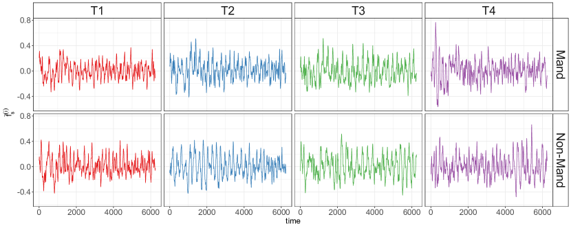
Formally, let $f^{(i)}_{s,m}(t)$ denote the FFR in the time domain, representing the brain activity of subject $i$ at time $t$ under the exposure to stimulus $s$ in the measurement $m$. We denote by $\bar{f}^{(i)}_{s}(t)=\sum_{m=1}^{1000}f^{(i)}_{s,m}(t)/1000$ the average over repeated measurements (as shown in Figure 1) and by $\text{SSE}^{(i)}_{s}(t)=\sum_{m=1}^{1000}\{f^{(i)}_{s,m}(t)-\bar{f}^{(i)}_{s}(t)\}^{2}$ the sum of squared errors at time $t$ for subject $i$ and stimulus $s$. Thus, as a measure of noise for the measurements at time $t$ in subject $i$ under the exposure to stimulus $s$, we use the estimated standard deviation $\widehat{\sigma}_{s}^{(i)}(t)=\{\text{SSE}^{(i)}_{s}(t)/(1000-1)\}^{1/2}$; and as a measure of individual dispersion at time $t$, the average of these standard deviations across stimuli $\widehat{\sigma}^{(i)}(t)=\sum_{s=1}^{S}\widehat{\sigma}_{s}^{(i)}(t)/S$. Finally, we rescale the average empirical distances at time $t$ by these estimated noise variances that cannot be explained by the average FFR, i.e., $\tilde{f}^{(i)}_{s}(t)=\bar{f}^{(i)}_{s}(t)/\widehat{\sigma}^{(i)}(t)$. By rescaling the Euclidean distances between average brain activities by the corresponding language group’s inherent noise levels in this manner, we allow for biologically meaningful comparisons of the brain’s ability to distinguish different auditory stimuli across subjects.

Figure 2 shows the average distances between stimuli in the two populations. We can see that, although there are population-specific characteristics due to language, e.g., the recorded Mandarin speaker distances are better differentiated across pairs of tones than the ones from the non-Mandarin populations, there are also strongly shared patterns across populations, e.g., the pair $\{2,3\}$ and $\{2,4\}$ are well-separated pairs of tones while the pairs $\{1,4\}$ and $\{1,2\}$ are the closest in both populations.

Figure 2: Tone neural distance data: Mean (intra-populations cross-subjects) FFR distances between different Mandarin tones.

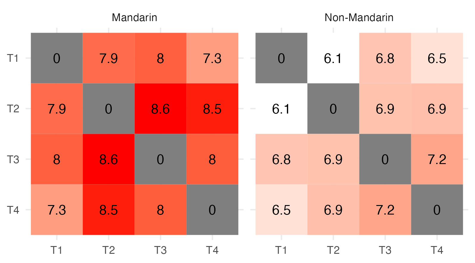
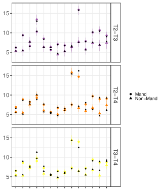
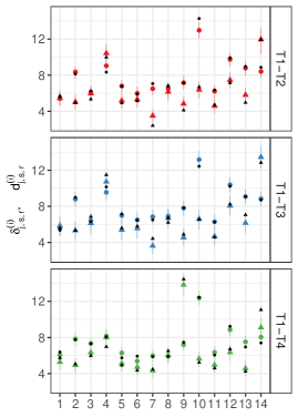
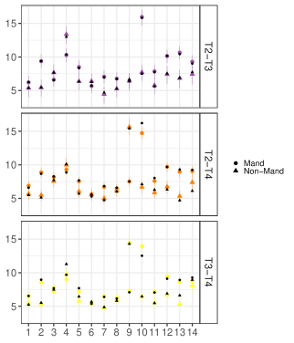
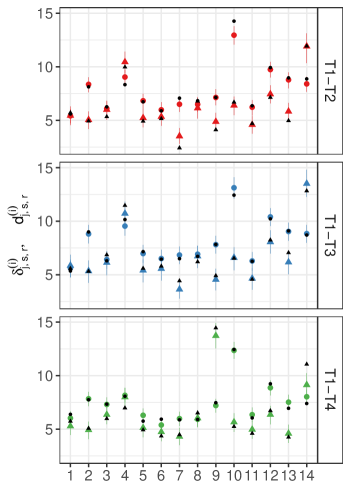
Figure 8 reports the individual tone distances, showing that there is also substantial individual variability within populations. Note also a higher within-group variability in the non-Mandarin population as expected.

We are interested in using MDS to learn the shared geometry of the lower-dimensional latent space representing these tones in the human brain across language groups and individuals while also assessing how this space varies across groups and individuals.

3 Mixed Multidimensional Scaling

In MDS, the observed distances between stimuli $s$ and $r$, namely $d_{s,r},r<s,r=1,\dots,S-1,s=2,\dots,S$, are noisy measurements of latent distances $\delta_{s,r}$’s computed in a lower $H$-dimensional feature space ($H<S$).

As in Nguyen and Holmes (2017) and Yanchenko and Hoff (2020), we assume a Gamma likelihood for the observed distances to perform our model-based MDS. However, motivated by the application, we allow for individual differences at the level of the latent features. We also consider different variances in the likelihood terms to take into account the heterogeneity of the noise levels between the two populations observed in the data.

More precisely, we denote by $d_{j,s,r}^{(i)}$ the distance between the $s^{th}$ and the $r^{th}$ stimuli ($r<s$) for the $i^{th}$ individual from the $j^{th}$ group and we assign a Gamma likelihood for the observed distances

$$d_{j,s,r}^{(i)}\overset{ind}{\sim}\hbox{Ga}\left(\texttt{mean}=\delta_{j,s,r}^{(i)},\,\texttt{var}=\sigma_{\epsilon,j}^{2}\right).$$ (1)

In the context of the experiment described in Section 2, $j=1$ and $j=2$ refer to the Mandarin-speaking group and the non-Mandarin-speaking group, respectively. The gamma likelihood is parametrized in terms of mean and variance to ease the interpretation of the latent parameters and it is centered around the underlying individual denoised distances $\delta_{j,s,r}^{(i)}$ which can vary across subjects within and across the two populations. The variance term $\sigma_{\epsilon,j}^{2}$ varies across groups allowing for different noise levels in the different populations.

The underlying individual distance $\delta_{j,s,r}^{(i)}$ is a function of $H$ unobserved individual features $\eta_{j,s,h}^{(i)}$, such as

$$\delta_{j,s,r}^{(i)}=\sqrt{\sum_{h=1}^{H}\left(\eta_{j,s,h}^{(i)}-\eta_{j,r,h}^{(i)}\right)^{2}},$$ (2)

where the number of latent features $H$ is smaller than the number of original stimuli $S$. Here $\mbox{\boldmath$\eta$}_{j,s}^{(i)}=(\eta_{j,s,1}^{(i)},\dots,\eta_{j,s,H}^{(i)})^{\rm T}$ denotes the latent vector with the feature values for the $s^{th}$ stimulus for the $i^{th}$ individual belonging to the $j^{th}$ populations. Finally, we put an inverse-gamma prior to learn the group-specific variance terms

$$\sigma_{\epsilon,j}^{2}\overset{ind}{\sim}\mbox{Inv-Ga}\left(\texttt{mean}=\mu_{\sigma^{2}_{\epsilon,j}},\,\texttt{var}=\sigma^{2}_{\sigma^{2}_{\epsilon,j}}\right).$$ (3)

3.1 Latent Features

Our modeling efforts concentrate henceforth on flexibly characterizing the latent features $\eta_{j,s,h}^{(i)}$. We model $\eta_{j,s,h}^{(i)}$ as a product of latent features shared across populations and subjects, $\eta_{j,s}$, and multiplicative coefficients specific to population $j$ and subject $i$ within population $j$. That is, we let

$$\eta_{j,s,h}^{(i)}=w_{j,h}^{(i)}\,w_{j}\,\eta_{s,h}.$$ (4)

The subject-specific random coefficient $w_{j,h}^{(i)}$ varies across features $h$ allowing variation, and thus importance, of the dimensions across individuals between and within populations. We also allow a group-specific random coefficient $w_{j}$ that introduces more heterogeneity between subjects across groups than within groups, coherently with neuroscientific knowledge. Here, we assume the populations under consideration to be mutually exclusive. The weights $w_{j,h}^{(i)}$ do not really vary with the population index $j$ but the index $j$ is still included here to distinguish between the individuals from different populations: $w_{1,h}^{(1)}$ corresponds to individual 1 in population 1, and $w_{2,h}^{(1)}$ corresponds to individual 1 in population 2.

Note that since $w_{j}$ is not indexed by the latent feature, it can be interpreted as a population-specific multiplicative term for the latent distance, i.e.,

$$\delta_{j,s,r}^{(i)}=w_{j}\sqrt{\sum_{h=1}^{H}\left(w_{j,h}^{(i)}\,\eta_{s,h}-w_{j,h}^{(i)}\,\eta_{r,h}\right)^{2}}.$$ (5)

In this way, $w_{j}$ allows us to rescale the distances in the different groups, and introduce group-level variability, similarly to the hierarchical Bayesian multidimensional scaling by Yanchenko and Hoff (2020).

In addition, we also allow for individual differences $w_{j,h}^{(i)}$ that can change the feature values across different features $h$. Importantly, this allows different subjects to have individual differences that are not the same across the features and also to assign different importance to the feature dimension $h$. Note that the fact that different subjects weigh differently the dimensions, for instance, according to language exposure, is a theory strongly believed and accepted in the auditory neuroscience literature (Gandour and Harshman, 1978; Gandour, 1983; Chandrasekaran et al., 2007a, b).

Finally, in order to learn the subjects’ and the two populations’ variations, we specify an inverse gamma distribution on their squares with hyper-parameters $a_{w}$ and $b_{w}$ such that the multiplicative terms have the mean equal to $1$ and a large variance equal to $10$. That is,

$$\begin{split}w_{j}^{-2}\overset{iid}{\sim}\text{Ga}\left(\texttt{shape}=a_{w},\texttt{rate}=b_{w}\right),\\ {w_{j,h}^{(i)}}^{-2}\overset{iid}{\sim}\text{Ga}\left(\texttt{shape}=a_{w},\texttt{rate}=b_{w}\right).\end{split}$$ (6)

Here we parametrize the Gamma distribution in terms of shape and rate hyper-parameters to ease the update of the hyper-parameters in the conjugate full conditionals. If the multiplicative terms $w_{j}$ and $w_{j,h}^{(i)}$ are equal to $1$, the MDS model ignores population and individual differences entailing the same latent feature values for the stimulus $s$ for all subjects within and across the two populations.

3.2 Model Identifiability

Our multiplicative individual effects make the latent feature space identifiable with respect to rotations, allowing for stronger interpretations of the latent features. To see this, note that re-weighting the latent features can be seen as a multiplication of the matrix of the features with a diagonal matrix of weights. Therefore, if we rotate the axes (aside from the special case of permutations of the axes and the subclass of signed permutations that can be represented as rotation), the weight matrix would not be diagonal anymore which is not permissible in our model. Therefore, it allows the axes of the latent features to be identified uniquely and not be affected by rotation invariance.

More precisely, let ${\mathbf{H}}^{(i)}_{j}=((\eta_{j,s,h}^{(i)}))\in{\mathbf{R}}^{H\times S}$, $i=1,\ldots,n_{j},\,j=1,\ldots,J$ be the individual latent feature matrices, ${\mathbf{W}}_{j}^{(i)}=w_{j}\,\hbox{diag}(w_{j,1}^{(i)},\ldots,w_{j,H}^{(i)})\in{\mathbf{R}}^{H\times H}$, $i=1,\ldots,n_{j},\,j=1,\ldots,J$ be the corresponding diagonal weight matrices, and ${\mathbf{H}}=((\eta_{s,h}))\in{\mathbf{R}}^{H\times S}$ be the shared latent feature matrix. Then, we can rewrite ${\mathbf{H}}^{(i)}_{j}=\mathbf{W}_{j}^{(i)}{\mathbf{H}}$. Now, let $\mathbf{R}\in{\mathbf{R}}^{H\times H}$ be a rotation matrix. If we rotate the individual features as $\mathbf{R}{\mathbf{H}}^{(i)}_{j}=\mathbf{R}\mathbf{W}_{j}^{(i)}{\mathbf{H}}$, it will not change the implied latent distances $\delta_{j,s,r}^{(i)}$, but the new individual weight matrices $\mathbf{W}_{j}^{(i),\text{new}}=\mathbf{R}\mathbf{W}_{j}^{(i)}$ are in general not diagonal anymore. This is why the individual weights, which are shared across stimuli, make the latent feature space identifiable in INDSCAL contrary to standard MDS analysis. See Carroll and Chang (1970) for further discussions.

The latent features $\eta_{j,s,h}^{(i)}$ are however still invariant to signed permutations and translations that preserve the latent distances $\delta$ (even if the axes are identifiable and cannot arbitrary rotated as discussed above). We address this issue via a post-processing scheme discussed later in Section 4.3.

Moreover, we note that the latent distances $\delta_{j,s,r}^{(i)}$ and group-specific variance terms $\sigma_{\epsilon,j}^{2}$ are identifiable. We rely here on the standard definition of identifiability of Basu (2004) as stated in Swartz et al. (2004). Then, focusing on the identifiability of the parameters $\widetilde{\mbox{\boldmath$\theta$}}=\{\delta_{j,s,r}^{(i)},\,\sigma_{\epsilon,j}^{2},\,i=1,\ldots,\,n_{j},j=1,\ldots,J,\,s=1,\ldots,S,\,r=1,\ldots,S\}$. Therefore, identifiability of $\widetilde{\mbox{\boldmath$\theta$}}$ follows noting the following moments identities

$$\mathbb{E}(d_{j,s,r}^{(i)}\mid\widetilde{\mbox{\boldmath$\theta$}})=\delta_{j,s,r}^{(i)},~{}~{}~{}\hbox{var}(d_{j,s,r}^{(i)}\mid\tilde{\mbox{\boldmath$\theta$}})=\sigma_{\epsilon,j}^{2}.$$

3.3 Prior Specification

To flexibly learn the shared latent features $\eta_{s,h}$, we adapt the multiplicative gamma process (MGP) introduced by (Bhattacharya and Dunson, 2011) for ordinary factor analysis that allows estimating the latent features with stochastically diminishing order of importance.

Specifically, we assume a Gaussian distribution for the shared feature component $\eta_{s,h}$ whose variance varies across stimuli $s$ and dimension $h$

$$\eta_{s,h}\overset{ind}{\sim}\hbox{Normal}\left(\texttt{mean}=0,\,\texttt{sd}=\phi_{s,h}^{-1/2}\,\tau_{h}^{-1/2}\right),$$ (7)

The precision parameter of the shared component $\eta_{j,s}$ follows the MGP

$$\phi_{s,h}\overset{iid}{\sim}\hbox{Ga}\left(\texttt{shape}=\nu/2,\texttt{rate}=\nu/2\right),$$ (8)

$$\tau_{h}=\prod_{l=1}^{h}\delta_{l},\quad\delta_{l}\overset{ind}{\sim}\hbox{Ga}\left(\texttt{shape}=a_{h},\,\texttt{rate}=1\right),$$ (9)

where $a_{h}=a_{2}$ for $h\geq 2$. The MGP prior shrinks the latent features increasingly towards zero as the dimension $h$ increases. This implies that the prior favors a few relevant features, shrinking the rest to zero, while also inducing a probabilistic ranking of the relevant features such that on average the first feature explains more variability than the second one, and so on, coherent with the current understanding of the brain’s behavior.

We follow Durante (2017) recommendations for the choice of the hyper-parameters of the MGP. In particular, we set $a_{1}=2$ and $a_{2}=3$ since they induce the desired prior shrinkage. More precisely, they induce an order in the probability of the dimensions in a neighborhood around zero (Lemma 2 in Durante (2017)).

3.4 Model Reparametrization

We can reparametrize the model in terms of the individual latent features $\eta_{j,s,h}^{(i)}$. Integrating out the shared dimensions $\eta_{s,h}$, we obtain

$$\eta_{j,s,h}^{(i)}\sim\hbox{Normal}\left(\texttt{mean}=0,\,\texttt{sd}={w_{j,h}^{(i)}}\,w_{j}\,\phi_{s,h}^{-1/2}\,\tau_{h}^{-1/2}\right).$$ (10)

This parameterization allows restating the probabilistic statements directly in terms of one of the main quantities of interest, namely the individual specific latent features. Note that, by the definition in (4), the $\eta_{j,s,h}^{(i)}$’s in (10) are dependent on each other since they share the same latent $\eta_{s,h}$’s. That is, $\eta_{j,s,h}^{(i)},i=1,\ldots,n_{j},j=1,\ldots,J,s=1,\ldots,S$ belong to the span of the vectors $\eta_{s,h},s=1,\ldots,S$. This is consistent with our goal to infer a common latent features’ space across groups as well as subjects.

4 Posterior Inference

Posterior inference is performed via samples drawn by an MCMC algorithm which exploits conditional conjugacy of the parameters when available. When sampling from the full conditionals is not straightforward, we exploit adaptive Metropolis schemes (Roberts and Rosenthal, 2009). The details are discussed in the next subsection.

4.1 MCMC Algorithm

(1) Sample $\delta_{1}$ from $p(\delta_{1}\mid\cdots)$

$$=\hbox{Ga}\bigg{(}\texttt{shape}=a_{1}+\frac{SH}{2},\,\texttt{rate}=1+\frac{1}{2}\sum_{l=1}^{H}\tau_{l}^{(1)}\sum_{s=1}^{S}\phi_{s,l}\eta_{s,l}^{2}\bigg{)}.$$

(2) Sample $\delta_{h}$ from $p(\delta_{h}\mid\cdots)$

$$=\hbox{Ga}\bigg{(}\texttt{shape}=a_{h}+\frac{S(H-h+1)}{2},\,\texttt{rate}=1+\frac{1}{2}\sum_{l=h}^{H}\tau_{l}^{(h)}\sum_{s=1}^{S}\phi_{s,l}\eta_{s,l}^{2}\bigg{)},$$

where $\tau_{l}^{(h)}=\prod_{t=1,\,t\neq h}^{l}\delta_{t}$, for $l=1,\ldots H$.

(3) Sample $\phi_{s,h}$ from

$$p(\phi_{s,h}\mid\cdots)=\hbox{Ga}\bigg{(}\texttt{shape}=\frac{\nu+1}{2},\,\texttt{rate}=\frac{\nu+\tau_{h}\eta_{s,h}^{2}}{2}\bigg{)}.$$

(4) Sample $\eta_{s,h}$ from

$$\begin{split}p(\eta_{s,h}\mid\cdots)&\propto{\cal N}\left(\eta_{s,h}\mid\texttt{mean}=0,\,\texttt{sd}=\phi_{s,h}^{-1/2}\tau_{h}^{-1/2}\right)\\ &\quad\prod_{j=1}^{J}\prod_{i=1}^{n_{j}}\prod_{r<s}\hbox{Ga}\left(d_{j,s,r}^{(i)}\mid\texttt{mean}=\delta_{j,s,r}^{(i)},\,\texttt{var}=\sigma_{\epsilon,j}^{2}\right).\end{split}$$

We perform an adaptive MH step (Roberts and Rosenthal, 2009) with random-walk univariate Gaussian proposal.

(5) Sample $\sigma^{2}_{\epsilon,j}$ from

$$\begin{split}p\left(\sigma^{2}_{\epsilon,j}\mid\cdots\right)&\propto\mbox{inv-Ga}\left(\sigma^{2}_{\epsilon,j}\mid\texttt{mean}=\mu_{\sigma^{2}_{\epsilon,j}},\,\texttt{var}=\sigma_{\sigma^{2}_{\epsilon,j}}\right)\\ &\quad\prod_{i=1}^{n_{j}}\prod_{s=2}^{S}\prod_{r=1}^{s-1}\hbox{Ga}\left(d_{j,s,r}^{(i)}\mid\texttt{mean}=\delta_{j,s,r}^{(i)},\,\texttt{var}=\sigma_{\epsilon,j}^{2}\right).\end{split}$$

We perform an adaptive MH step with random-walk Gaussian proposal for $\hbox{log}(\sigma^{2}_{\epsilon,j})$.

(6) Sample $w_{j,h}^{(i)}$ from

$$\begin{split}p\left(w_{j,h}^{(i)}\mid\cdots\right)\propto\mbox{inv-Ga}\left(w_{j,h}^{(i)}\mid\texttt{shape}=a_{w},\,\texttt{rate}=b_{w}\right)\\ \prod_{s=2}^{S}\prod_{r=1}^{s-1}\text{Ga}\left(d_{j,s,r}^{(i)}\mid\texttt{mean}=\delta_{j,s,r}^{(i)},\,\texttt{var}=\sigma_{\epsilon,j}^{2}\right).\end{split}$$

We perform an adaptive MH step with random-walk Gaussian proposal for $\hbox{log}(w_{j,h}^{(i)})$. (7) Sample $w_{j}$ from

$$\begin{split}p(w_{j}\mid\cdots)\propto\mbox{inv-Ga}\left(w_{j}\mid\texttt{shape}=a_{w},\,\texttt{rate}=b_{w}\right)\\ \prod_{i=1}^{n_{j}}\prod_{s=2}^{S}\prod_{r=1}^{s-1}\text{Ga}\left(d_{j,s,r}^{(i)}\mid\texttt{mean}=\delta_{j,s,r}^{(i)},\,\texttt{var}=\sigma_{\epsilon,j}^{2}\right).\end{split}$$

We perform an adaptive MH step with a random-walk Gaussian proposal for $\hbox{log}(w_{j})$.

4.2 Selecting the Number of Features

Our Bayesian mixed multidimensional scaling model allows performing dimensionality reduction by setting $H<S$. If we choose a conservative (i.e., larger than needed) upper bound $H^{+}$, the model allows us to give relevant importance to a few latent features $H<H^{+}$ and small importance to the remaining $H^{+}-H$ latent features. Here, we can think of $H$ as the effective number of features so that the contribution from adding additional features in reconstructing a denoised version of the observed distance matrices is negligible. However, running the MCMC for an upper bound $H^{+}$ larger than needed can be computationally inefficient. Finding the number of relevant latent features $H$ can therefore be helpful in reducing costs. Finding $H$ can also be of inferential interest itself.

To address this, we define $D(t)$ to be the average (across subjects) Frobenius distance between the observed distance matrices $((d_{j,s,r}^{(i)}))$ and the corresponding denoised latent distance matrices $((\delta_{j,s,r}^{(i)}))$ sampled in iteration $t$ divided by the Frobenius norm of the observed distance matrix in order to rescale the absolute distance by the ‘dimension’ of the problem. We set, according to the noise level in the measurements, a threshold $D_{T}$. In particular, we noted that $D_{T}=0.9$ favors a parsimonious latent space that is able to reconstruct well all the individual observable distances in our motivating neural tone distance experiment as shown in Figure 8. We perform the following steps with probability $p(t)=\exp(\alpha_{0}+\alpha_{1}t)$ at iteration $t$ where $\alpha_{0}\geq 0$ and $\alpha_{1}<0$ such that the adaptations occur often at the beginning of the chains, but decreases in frequency exponentially fast as the chain settles in. At the $t^{th}$ iteration, if the current latent features are not sufficient to recover the distances well, i.e., $D(t)>D_{T}$, we set $H(t+1)=H(t)+1$ and add a latent feature $\eta_{s,H(t)+1}$. Otherwise, we set $H(t+1)=H(t)-1$ and delete the feature $\eta_{s,H(t)}$. The other parameters are modified accordingly. When we add a feature, we sample the parameters from the prior distribution. Otherwise, we retain parameters corresponding to the non-redundant features.

The adaptive method allows, in a single run, to perform posterior inference on the individual and population latent distances, $\delta_{j,s,r}^{(i)}$ and $\delta_{j,s,r}$, together with selecting the number of features, with the convergence of the chain guaranteed by the diminishing probability condition (Roberts and Rosenthal, 2007). If, as in our motivating auditory neuroscience application, one is interested in performing inference on the actual latent features, we can fix the number of active dimensions $H$ selected in a preliminary run of the MCMC chain or in an initial set of iterations of the chain after burn-in. In this way, we have the same number of features, $H$, sampled in the final stages of the chain that we can use to perform posterior inference on the latent features after solving the identifiability issues as described in the next section. Finally, as in Bhattacharya and Dunson (2011), we can perform uncertainty quantification on the number of features around the point estimate of $H$, in our case the median of the sampled values $H(t)$ after burn-in, via credible intervals.

4.3 Post-processing for Feature Identifiability

In MDS, inference on the latent features $\eta_{j,s,h}^{(i)}$’s is challenging due to identifiability issues – while the reconstructed distances are identifiable, the features themselves are not. Importantly, as discussed in Section 3.2, our construction overcomes the rotation invariance issue of the latent dimensions that affects standard MDS methods. However, although the latent feature axes are now identifiable, the values of the latent features are still only unique up to translations and signed permutation of the axes (e.g., label switching of the dimensions and reflection). This makes the posterior summaries of the sampled latent features computed from the MCMC samples, e.g., the posterior median, not meaningful.

To address this, we adapt recent post-processing techniques introduced to solve similar identifiability issues in Bayesian latent factor models by Papastamoulis and Ntzoufras (2022). Specifically, we first solve the translation invariance by re-centering in each iteration $\eta_{s,h}$ around the origin, i.e., such that $\sum_{s=1}^{S}\eta_{s,h}=0$ and we translate the $\eta_{j,s,h}^{(i)}$’s accordingly. Then, we rescale the weights and the shared feature values such that $\eta_{j,s,h}=\sum_{i=1}^{n_{j}}\eta_{j,s,h}^{(i)}/n_{j}$, $\eta_{s,h}=\sum_{j=1}^{J}\sum_{i=1}^{n_{j}}\eta_{j,s,h}^{(i)}/n$ (i.e., such that $\sum_{i=1}^{n_{j}}w_{j}w_{j,h}^{(i)}=n_{j}$), and $\sum_{j=1}^{J}w_{j}=J$. Finally, we apply signed permutation matrices that align the samples of $\eta_{s,h}$ and accordingly the $\eta_{j,s,h}^{(i)}$’s across iterations.

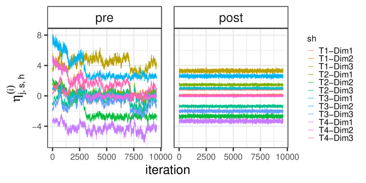
Based on these adjusted samples, we can compute meaningful posterior summaries for inference for each subject that are comparable across subjects and groups, e.g., median posterior values and credible intervals. Trace plots of the latent features before and after post-processing that solve the identifiability issues are shown in Figure 6 below.

4.4 MCMC Diagnostics

The results reported in this article are all based on $10^{5}$ MCMC iterations with the initial $4\,000$ iterations discarded as burn-in. The remaining samples were further thinned by an interval of 10. We programmed everything in R. The analyses are performed with a Lenovo ThinkStation P340 Tiny Workstation with 32Gb RAM (Windows 10), using a R version 4.1.2. For the real data set, the MCMC algorithm takes 28 minutes and 32 seconds and the post-processing algorithm takes 1 hour and 11 minutes. See the supplementary materials for further details and diagnostics.

5 Simulation Studies

In this section, we discuss the results of some synthetic numerical experiments. In designing the simulation scenarios, we have tried to closely mimic our motivating ‘brain activities distances between tones’ data set. We thus consider distances between $S=4$ stimuli from $n=28$ subjects recorded in two groups with cardinalities $n_{1}=14$ and $n_{2}=14$. We set the observed distances $d_{j,s,r}^{(i)}$ close to values that correspond to the estimated quantities for the real data set, i.e., the simulated distances can be reconstructed from 3-dimensional latent space.

Figure 3 shows that the three shared latent features recover the observed distances at the population level quite well. Note that the population distance parameters $\delta_{j,s,r}$ are obtained as average within the population of the individual parameters, i.e., $\delta_{j,s,r}=\sum_{i=1}^{n_{j}}\delta_{j,s,r}^{(i)}/n_{j}$. Moreover, Figure 4 suggests that we recover the denoised version of the empirical distances quite well at the individual level as well.

Figure 3: Results for synthetic distance data: Posterior medians and 90% credible intervals of the population latent distances $\delta_{j,s,r}$ between stimuli. Black squares represent the median observed distances in each population.

Figure 4: Results for synthetic distance data. Observed distances $d_{j,s,r}^{(i)}$ vs. posterior medians of the denoised distances, $\delta_{j,s,r}^{(i)}$, reconstructed from three shared dimensions.

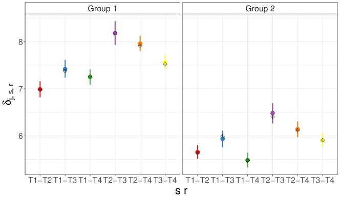
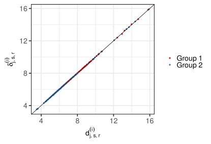
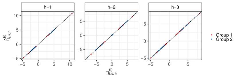
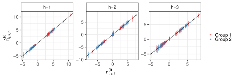
Figure 5 shows that our method allows us to recover the underlying latent features very efficiently. Here we align the signs of the true and the estimated latent features for identifiability. When it comes to permuting the dimension labels, however, we leave them undisturbed. We can do this since our method assigns decreasing importance to the dimensions, consistent with the data-generating truth, and we are able to identify the order of the axes after post-processing. Importantly, contrary to standard MDS methods, we do not need to arbitrarily rotate the latent space, since the directions are identifiable.

Figure 5: Results for synthetic distance data. True features $\eta_{j,s,r}^{(i)}$ vs. posterior medians of the latent features $\widehat{\eta}_{j,s,r}^{(i)}$.

MCMC diagnostics for the simulation experiments are similar to those shown for the real data analysis (see the next section) and hence are omitted. Figure 6 shows the trace plots of the individual latent features before and after applying the algorithm to solve the identifiability issue in the first subject. We can see how the procedure described in Section 4.3 identifies the posterior samples of the different latent features allowing meaningful inference and comparison at the level of the latent features $\eta_{j,s,h}^{(i)}$.

Figure 6: Diagnostics for synthetic distance data. Trace plots of the individual features $\eta_{j,s,h}^{(i)}$ sampled in the first subject of group 2 pre- and post-processing.

6 Application to Neural Tone Distances

In this section, we discuss the results produced by our method applied to the two populations’ tone distances data described in Section 2. Our inference goals, we recall, include understanding similarities in terms of stimuli distances between subjects within and across Mandarin and non-Mandarin listeners as well as comparing individual and group latent feature values. The selected number of dimension $H$ is $3$ since after the burn-in the adaptive criterion discussed in Section 4.2 suggested to sample from $H=2$ in $5\%$ of the MCMC iterations and from $H=3$ in $95\%$ of the iterations.

Figure 7 shows the posterior point estimates and $90\%$ credible intervals of the group distances $\delta_{j,s,r}$ between each of the $\binom{4}{2}=6$ pairs of tones. We can see similar ranking (across groups $j$’s) of the pairs of tones according to $\delta_{j,s,r}$. Indeed, after discarding individual differences, in both populations, the pairs of Mandarin tones $\{2,3\}$ and $\{2,4\}$ exhibited the strongest degree of neural dissimilarity whereas pairs $\{1,2\}$ and $\{1,4\}$ exhibited the strongest degree of neural similarity. These findings are corroborated by empirical evidence from the preliminary analysis of the data in Section 2. Note that although the rankings between the point estimates are similar, they are not exactly the same across the two groups and that there is more uncertainty, quantified via the posterior credible intervals, in the non-Mandarin group due to greater variability across these individuals. Moreover, consistent with recent neuroscience work (Llanos et al., 2017; Reetzke et al., 2018), we observe a better separation between neural representations of tones in the group of native listeners of Mandarin Chinese, relative to the group of non-native listeners of Mandarin Chinese.

Figure 7: Results for tone neural distance data. Posterior medians and 90% credible intervals of the group latent distances $\delta_{j,s,r}$ between stimuli.

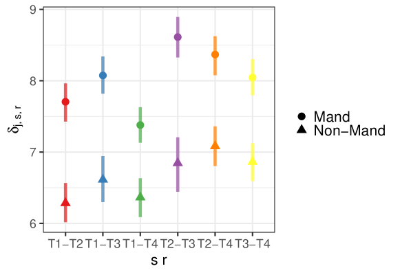
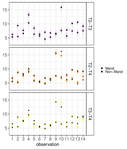
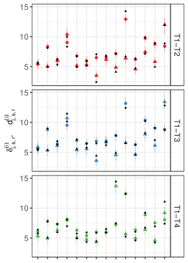
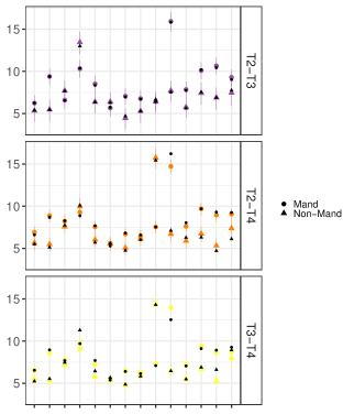
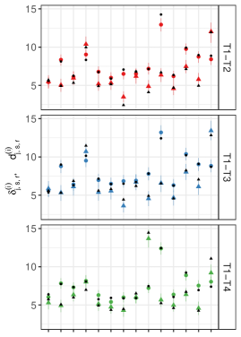
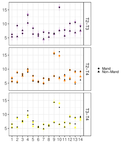
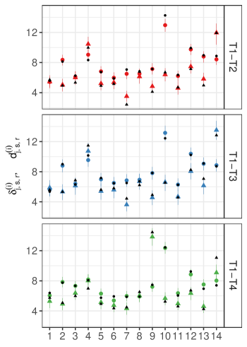
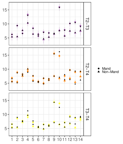
Figure 8 shows the posterior point estimates and $90\%$ credible intervals of the individual distances $\delta_{j,s,r}^{(i)}$ as well as the corresponding observed distances. We can see that three latent common features reconstruct the observed distances very well. This indicates that the neural encoding of differences between multidimensional neural representations can be captured using three latent dimensions.

We also note greater uncertainty in the estimates of the denoised individual distances for the non-Mandarin subjects. Note that our Bayesian model allows us to quantify such uncertainty via posterior credible intervals while also allowing us to perform proper individual and population comparisons.

Figure 8 also highlights the presence of some non-Mandarin speakers (e.g., subjects 7 and 11) that struggle to distinguish between neural responses to specific pairs of tones (e.g., {T1, T2} and {T2, T3}) more than other subjects in the same population.

Figure 8: Results for tone neural distance data. Posterior medians and 90% credible intervals of the individual latent distances $\delta_{j,s,r}^{(i)}$ between stimuli. Black points represent the observed distances $d_{j,s,r}^{(i)}$.

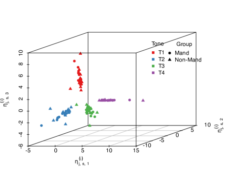
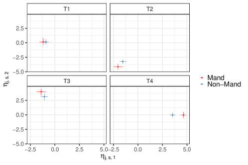
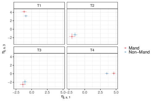
Importantly, by addressing the identifiability issues, we are also able to perform inference on the group and individual latent feature values that reconstruct the distances. Notably, the model can be also used to infer structural differences at the level of the evoking stimuli with a high degree of specificity. These differences are depicted in Figure 9. In this figure, the first dimension encodes the difference between the neural representations of T4 (high-falling pitch) and the other tones: T1 (high-level pitch), T2 (low-rising pitch), and T3 (low-dipping pitch). Because T4 is the high-falling tone, this dimension reflects the neural encoding of differences in pitch direction (falling vs. level, rising, and dipping pitch). In contrast, the second dimension encodes the difference between the neural representations of T3 and T2. Because T3 and T2 are the low-dipping and low-rising tones, respectively, this dimension captures neural differences in pitch direction for low-onset tones (dipping vs. rising pitch). Lastly, the third dimension encodes the difference between the neural representations of T1 and T3. Because these tones are the ones with higher (T1) and lower (T3) pitch on average, this dimension may reflect the neural encoding of differences in pitch range (high vs. low range). Figure 9 also highlights the fact that the three latent features play the same role in the two populations and that the tones are more distinguished (i.e., $\eta_{j,s,h}$ more distant from $0$) in all the features in Mandarin native speakers. See also the supplementary materials for additional plots summarizing these results.

Figure 9: Results for tone neural distance data. Upper panel: 3-dimensional scatter plot of posterior medians of the population latent feature values $\eta_{j,s,h}$. Lower panel: 2-dimensional representation of the posterior medians and 90% credible intervals of the population latent feature values $\eta_{j,s,h}$ in the different populations.

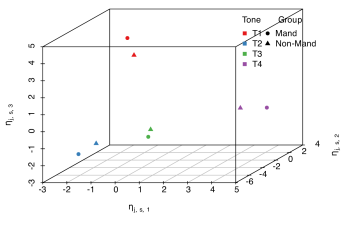
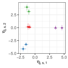
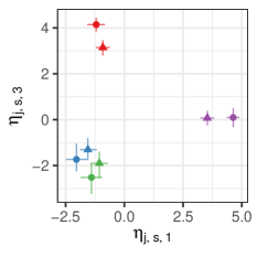
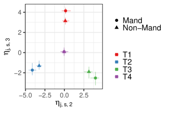
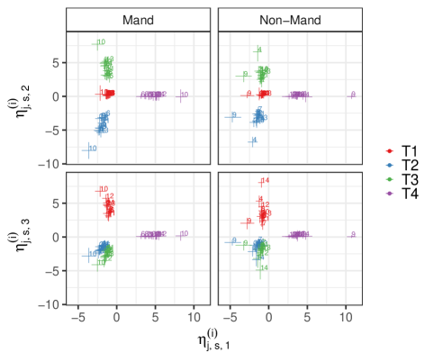
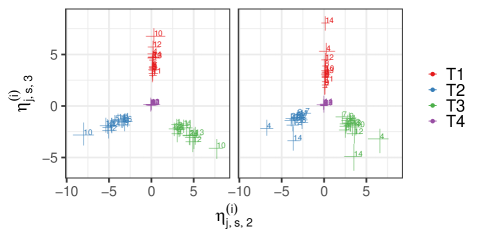
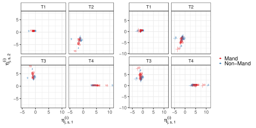
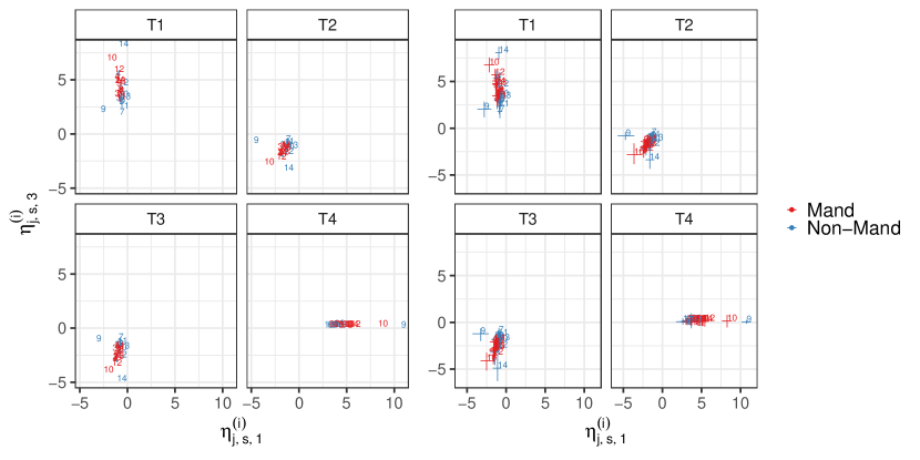
Figure 10 shows the positions of different subjects on the feature space within and across the two populations and tones and the associated $90\%$ credible interval, presented separately for clarity. We see that at the individual levels as well: The first feature is mainly useful to distinguish tone $4$. The second and third features are mainly useful to represent the other tones both at population and individual levels. Moreover, although we note some similarities between Mandarin and non-Mandarin speakers, as expected, there is more individual variability in the latent features for non-native speakers. The individual latent features in Figure 10 also identify a few non-Mandarin speakers who struggle to distinguish the Mandarin tones, especially in the third dimension.

Figure 10: Results for tone neural distance data. Upper panel: 3-dimensional scatter plot of posterior medians of the individual latent features $\eta_{j,s,h}^{(i)}$ between stimuli in the two populations. Lower panels: 2-dimensional representation of the posterior medians and 90% credible intervals of the individual latent feature values $\eta_{j,s,h}^{(i)}$ in the different populations.

6.1 MCMC Diagnostics

Here we present some convergence diagnostics for the MCMC sampler for the Mandarin tone neural distance data analysis.

Figure 11: Trace plots of $\delta_{j,s,r}$, the latent distances between different pairs of tones between the two populations.

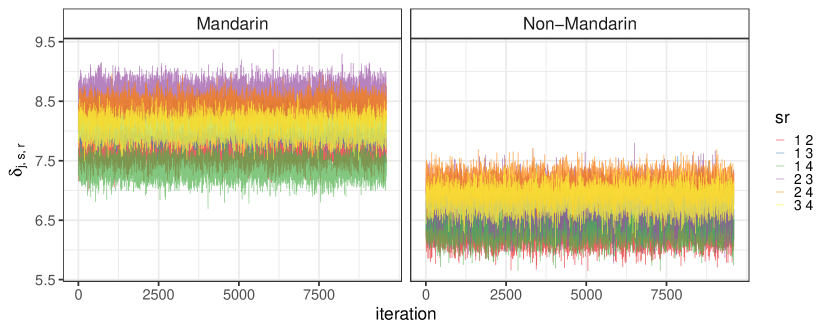
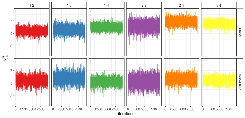
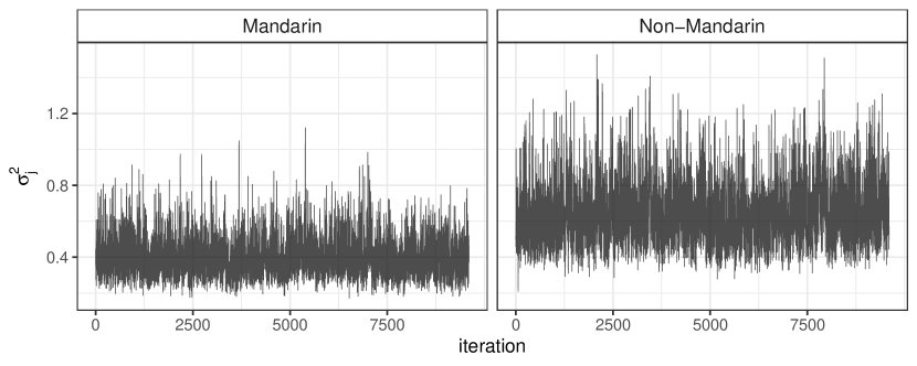
Figure 11 shows the trace plots for the population-specific distances $\delta_{j,s,r}$ between the different tones. The trace plots suggest a good performance of the MCMC algorithm in sampling from the posterior distributions. Figure 4 of the supplementary materials shows the trace plots for the individual tone distances in a Mandarin and a non-Mandarin listener. Finally, Figure 5 of the supplementary materials shows the trace plots of population-specific variances $\sigma^{2}_{j}$. These trace plots do not seem to indicate any convergence or mixing issues.

6.2 Identifiability Diagnostics

Posterior inference on the individual latent features $\eta_{j,s,h}^{(i)}$ is only meaningful after solving the identifiability issues explained in Section 3.2.

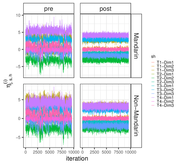
Figure 12 shows the trace plot of the MCMC samples of the individual latent features $\eta_{j,s,h}^{(i)}$ before and after the post-processing algorithm for one Mandarin-speaking and one non-Mandarin-speaking listener. The trace plot strongly suggests that the post-processing procedure was able to solve the identifiability issue as expected.

Figure 12: Diagnostic for tone neural distance data. Upper panel: Trace plots of the individual features $\eta_{j,s,h}^{(i)}$ for one Mandarin-speaking listener pre and post-processing. Lower panel: Trace plots of the individual features $\eta_{j,s,h}^{(i)}$ for one non-Mandarin-speaking listener pre and post-processing.

7 Discussion

In this study, we proposed a novel mixed effects MDS model for multi-populations and multi-subjects distances. Our research was motivated primarily by auditory neuroscience experiments where scientists are interested in understanding the structural differences in the latent representation of speech sounds in the brain. We looked specifically at the representation of Mandarin Chinese tones in two groups of people - one comprising native Mandarin speakers and the other comprising native English speakers who were unfamiliar with these tones. Our proposed model allowed us to interpret and compare the latent features that reconstruct the denoised empirical distances across these two groups as well as across individuals within these groups. Furthermore, our model allowed us to infer structural differences between groups and stimuli along latent dimensions linked to the neural coding of specific stimulus differences. We found that, aside from some neural differences due to long-term exposure to tonal language in the Mandarin listeners, some behavior is shared across subjects in the two different human groups. We also identified some non-Mandarin speakers that struggled to distinguish the tones compared with other Mandarin and non-Mandarin speakers.

Our proposed approach advances the MDS literature significant steps forward, enabling neuroscientists to perform statistical comparisons across multi-subject and multi-population brain distances by mapping them to a biologically interpretable lower-dimensional common feature space where the latent axes are now all identifiable. Our proposal allows proper borrowing of information across populations and subjects, providing the means for a more comprehensive understanding of how the human brain processes speech signals. Importantly, going beyond just being used as a visualization tool in neuroscience research, our proposed MDS approach also allows for straightforward uncertainty quantification as well as data-driven selection of the number of latent features.

The scope of the proposed MDS approach is not restricted to auditory neuroscience problems but the model can be applied to model structural differences between neural representations of other sensory stimuli (e.g., visual signals) captured by neuroimaging technologies such as EEG, fMRI, and MEG. Prior neuroscience work (Kluender et al., 2019; Lewicki, 2002; Lotto and Holt, 2016; Stilp and Kluender, 2012) suggests that the neural coding of complex multidimensional sensory stimuli is informed by principles of dimensionality reduction. Our model could also be used to infer the latent neural dimensions needed by the human brain to encode differences between sensory signals and the impact of different kinds of experiences on the number of dimensions. Additionally, our approach can be used to address scientific problems in other fields such as in bioinformatics to find smaller dimensional biological relevant features that summarize the recorded single-cell RNA genetic expressions in several biomarkers, e.g., to extend classical MDS used in standard dimensionality reduction pipeline in bioinformatics research (Perraudeau et al., 2017).

Methodological extensions and topics of our ongoing research include incorporating covariates, accommodating asymmetric distance matrices, adaptations to longitudinal experiments capturing the dynamic evolution of the latent features, etc.

Funding

This work was supported in part by the National Science Foundation grant NSF DMS-1953712, National Institute on Deafness and Other Communication Disorders grants R01DC013315 and R01DC015504. G. R. has been partially supported by the Italian grant MUR, PRIN project 2022CLTYP4.

Supplementary Materials for
Bayesian Mixed Multidimensional Scaling
for Auditory Processing

Supplementary materials present additional figures of the results of the tone distances application and simulated data analysis and details on software and diagnostics.

S.1 Additional Figures: Neural Tone Distances

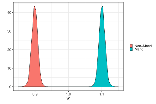
Figure S.1 shows the distribution of the posterior weights $w_{j}$ after post-processing in the two populations. Note that $w_{1}+w_{2}$ must be equal to $1$ and the population weight of the Mandarin-speaking population is higher than that of the non-Mandarin-speaking population coherently with the data and the results in the main manuscript.

Figure S.1: Results for tone neural distance data. Posterior density of the weights $w_{j}$ in the different populations.

Figures S.2 and S.3 show the posterior results for the population and individual latent features, respectively.

Figure S.2: Results for tone neural distance data. Posterior medians and 90% credible intervals of the population latent feature values $\eta_{j,s,h}$ in the different tones.

Figure S.3: Results for tone neural distance data. Left panels: Posterior medians of the individual latent features $\eta_{j,s,h}^{(i)}$ between stimuli in the different tones. Right panels: Posterior medians and 90% credible intervals of the individual latent feature values $\eta_{j,s,h}^{(i)}$ in the different tones.

Finally, Figures S.4 and S.5 show evidence of numerical convergence of the individual distance and population variance parameters.

Figure S.4: Diagnostic for tone neural distance data: Trace plot of latent individual distances between tones, $\delta_{j,s,r}^{(i)}$, in a Mandarin and non-Mandarin speaker.

Figure S.5: Diagnostic for tone neural distance data: Trace plots of population-specific variances $\sigma^{2}_{j}$.

S.2 Additional Figures: synthetic distance data

Figure S.6 compare the estimated individual latent features $\eta_{j,s,r}^{(i)}$ vs the simulation truth and show that the model recovers the underlying truth very well.

Figure S.6: Results for synthetic distance data. True features $\eta_{j,s,r}^{(i)}$ vs. posterior medians and 90% credible intervals of the latent features $\widehat{\eta}_{j,s,r}^{(i)}$.

S.3 Initialization and Convergence Diagnostics

The results in the main manuscript are obtained by initializing the individual latent features $\eta_{j,s,r}^{(i)}$, the population latent features $\eta_{s,r}$, and the individual weights $w_{j,h}^{(i)}$ (while $w_{j}=1$) in the MCMC chain with the INDSCAL estimates obtained using the R package multiway.

To assess convergence, we ran the analysis also with different MDS initialization schemes (function cmdscale in R) that do not allow for individual differences, i.e., $\eta_{j,s,r}^{(i)}=\eta_{s,r}$ and $w_{j,h}^{(i)}=w_{j}=1$ for all $i,j,h$. Specifically, we considered

• All subjects: computed from the average across all subjects’ distance matrices.

• Mandarin speakers: computed from the average across Mandarin speakers’ distance matrices.

• Non-Mandarin speakers: computed from the average across Non-Mandarin speakers’ distance matrices.

We show the results for the individual latent distances $\delta_{j,s,r}^{(i)}$ (which are identifiable before post-processing) with the different initialization in Figure S.7. The results for the different MDS and INDSCAL initializations are practically the same (also compared with Figure 8 in the main manuscript).

Figure S.7: Results for neural data. Posterior medians and 90% credible intervals of the individual latent distances $\delta_{j,s,r}^{(i)}$ between stimuli with different MDS initializations. Black points represent the observed distances $d_{j,s,r}^{(i)}$.

Moreover, standard convergence tests like Gelman and Rubin’s univariate (Gelman and Rubin, 1992) and multivariate (Brooks and Gelman, 1998) diagnostics for the individual latent distances $\delta_{j,s,r}^{(i)}$ were all very close to $1$, suggesting good convergence in all cases.

S.4 Sensitivity to the Multiplicative Gamma Prior Hyperparameters

The choice of the hyperparameters of the multiplicative Gamma prior is crucial to inducing dimensionality reduction in high-dimensional sparse setting (Durante, 2017). In our tone neural distance application with a small number of stimuli $S=4$, the results were very robust to their choices. Nonetheless, we used the values suggested in Durante (2017) (i.e., $a_{1}=2$ and $a_{2}=3$) to obtain the results reported in the main manuscript. We also performed a sensitivity analysis considering the other setting in Durante (2017) (i.e., $a_{1}=a_{2}=3$ and $a_{1}=1$, $a_{2}=2$). In all the settings $H=3$ latent dimensions were strongly suggested by the data. Specifically, the adaptive criterion discussed in Section 4.2 in the main paper suggested sampling from the $H=2$ case in about $5\%$ of the MCMC iterations and from the $H=3$ case in about $95\%$ of the MCMC iterations after the burn-in. We show the results for the individual latent distances $\delta_{j,s,r}^{(i)}$ (which are identifiable without post-processing) with the two additional hyperparameter settings (i.e., $a_{1}=a_{2}=3$ and $a_{1}=1$, $a_{2}=2$) in Figure S.8 below. These results are practically the same and coherent with the ones reported in Figure 8 of the main manuscript.

Figure S.8: Results for neural data. Posterior medians and 90% credible intervals of the individual latent distances $\delta_{j,s,r}^{(i)}$ between stimuli with different MDS initializations. Black points represent the observed distances $d_{j,s,r}^{(i)}$.

References

Brooks, S. P. and Gelman, A. (1998). General methods for monitoring convergence of
   iterative simulations. Journal of Computational and Graphical Statistics, 7, 434–455.

Durante, D. (2017). A note on the multiplicative gamma process. Statistics & Probability    Letters, 122, 198–204.

Gelman, A. and Rubin, D. B. (1992). Inference from iterative simulation using multiple
   sequences. Statistical Science, 7, 457–472.

References

- Basu (2004) Basu, A. P. (2004). Identifiability. Encyclopedia of Statistical Sciences.
- Bhattacharya and Dunson (2011) Bhattacharya, A. and Dunson, D. B. (2011). Sparse Bayesian infinite factor models. Biometrika, 98, 291–306.
- Bidelman et al. (2011) Bidelman, G. M., Krishnan, A., and Gandour, J. T. (2011). Enhanced brainstem encoding predicts musicians’ perceptual advantages with pitch. European Journal of Neuroscience, 33, 530–538.
- Brooks and Gelman (1998) Brooks, S. P. and Gelman, A. (1998). General methods for monitoring convergence of iterative simulations. Journal of Computational and Graphical Statistics, 7, 434–455.
- Caclin et al. (2005) Caclin, A., McAdams, S., Smith, B. K., and Winsberg, S. (2005). Acoustic correlates of timbre space dimensions: a confirmatory study using synthetic tones. The Journal of the Acoustical Society of America, 118, 471–482.
- Caclin et al. (2006) Caclin, A., Brattico, E., Tervaniemi, M., Näätänen, R., Morlet, D., Giard, M.-H., and McAdams, S. (2006). Separate neural processing of timbre dimensions in auditory sensory memory. Journal of Cognitive Neuroscience, 18, 1959–1972.
- Carroll and Chang (1970) Carroll, J. D. and Chang, J.-J. (1970). Analysis of individual differences in multidimensional scaling via an N-way generalization of “Eckart–Young” decomposition. Psychometrika, 35, 283–319.
- Chandrasekaran et al. (2007a) Chandrasekaran, B., Krishnan, A., and Gandour, J. T. (2007a). Mismatch negativity to pitch contours is influenced by language experience. Brain Research, 1128, 148–156.
- Chandrasekaran et al. (2007b) Chandrasekaran, B., Gandour, J. T., and Krishnan, A. (2007b). Neuroplasticity in the processing of pitch dimensions: a multidimensional scaling analysis of the mismatch negativity. Restorative Neurology and Neuroscience, 25, 195–210.
- Di Liberto et al. (2015) Di Liberto, G. M., O’Sullivan, J. A., and Lalor, E. C. (2015). Low-frequency cortical entrainment to speech reflects phoneme-level processing. Current Biology, 25, 2457–2465.
- Durante (2017) Durante, D. (2017). A note on the multiplicative gamma process. Statistics & Probability Letters, 122, 198–204.
- Feng et al. (2019) Feng, G., Yi, H. G., and Chandrasekaran, B. (2019). The role of the human auditory corticostriatal network in speech learning. Cerebral Cortex, 29, 4077–4089.
- Feng et al. (2021a) Feng, G., Gan, Z., Llanos, F., Meng, D., Wang, S., Wong, P. C. M., and Chandrasekaran, B. (2021a). A distributed dynamic brain network mediates linguistic tone representation and categorization. Neuroimage, 224, 1–13.
- Feng et al. (2021b) Feng, G., Li, Y., Hsu, S.-M., Wong, P. C. M., Chou, T.-L., and Chandrasekaran, B. (2021b). Emerging native-similar neural representations underlie non-native speech category learning success. Neurobiology of Language, 2, 280–307.
- Gandour (1983) Gandour, J. (1983). Tone perception in far eastern languages. Journal of Phonetics, 11, 149–175.
- Gandour (1978) Gandour, J. T. (1978). The perception of tone. In Tone, pages 41–76. Elsevier.
- Gandour and Harshman (1978) Gandour, J. T. and Harshman, R. A. (1978). Crosslanguage differences in tone perception: a multidimensional scaling investigation. Language and Speech, 21, 1–33.
- Gelman and Rubin (1992) Gelman, A. and Rubin, D. B. (1992). Inference from iterative simulation using multiple sequences. Statistical Science, 7, 457–472.
- Khalighinejad et al. (2017) Khalighinejad, B., da Silva, G. C., and Mesgarani, N. (2017). Dynamic encoding of acoustic features in neural responses to continuous speech. Journal of Neuroscience, 37, 2176–2185.
- Kluender et al. (2019) Kluender, K. R., Stilp, C. E., and Llanos, F. (2019). Long-standing problems in speech perception dissolve within an information-theoretic perspective. Attention, Perception, & Psychophysics, 81, 861–883.
- Krishnan et al. (2005) Krishnan, A., Xu, Y., Gandour, J., and Cariani, P. (2005). Encoding of pitch in the human brainstem is sensitive to language experience. Cognitive Brain Research, 25, 161–168.
- Krishnan et al. (2010) Krishnan, A., Gandour, J. T., and Bidelman, G. M. (2010). The effects of tone language experience on pitch processing in the brainstem. Journal of Neurolinguistics, 23, 81–95.
- Lewicki (2002) Lewicki, M. S. (2002). Efficient coding of natural sounds. Nature Neuroscience, 5, 356–363.
- Llanos et al. (2017) Llanos, F., Xie, Z., and Chandrasekaran, B. (2017). Hidden Markov modeling of frequency-following responses to Mandarin lexical tones. Journal of Neuroscience Methods, 291, 101–112.
- Llanos et al. (2021) Llanos, F., German, J. S., Gnanateja, G. N., and Chandrasekaran, B. (2021). The neural processing of pitch accents in continuous speech. Neuropsychologia, 158, 1–12.
- Lotto and Holt (2016) Lotto, A. J. and Holt, L. L. (2016). Speech perception: the view from the auditory system. In Neurobiology of Language, pages 185–194. Elsevier.
- Mesgarani et al. (2014) Mesgarani, N., Cheung, C., Johnson, K., and Chang, E. F. (2014). Phonetic feature encoding in human superior temporal gyrus. Science, 343, 1006–1010.
- Nguyen and Holmes (2017) Nguyen, L. H. and Holmes, S. (2017). Bayesian unidimensional scaling for visualizing uncertainty in high dimensional datasets with latent ordering of observations. BMC Bioinformatics, 18, 65–79.
- Nili et al. (2014) Nili, H., Wingfield, C., Walther, A., Su, L., Marslen-Wilson, W., and Kriegeskorte, N. (2014). A toolbox for representational similarity analysis. PLoS Computational Biology, 10, 1–11.
- Oh and Raftery (2001) Oh, M. S. and Raftery, A. E. (2001). Bayesian multidimensional scaling and choice of dimension. Journal of the American Statistical Association, 96, 1031–1044.
- Papastamoulis and Ntzoufras (2022) Papastamoulis, P. and Ntzoufras, I. (2022). On the identifiability of Bayesian factor analytic models. Statistics and Computing, 32, 1–29.
- Perraudeau et al. (2017) Perraudeau, F., Risso, D., Street, K., Purdom, E., and Dudoit, S. (2017). Bioconductor workflow for single-cell RNA sequencing: normalization, dimensionality reduction, clustering, and lineage inference. F1000Research, 6, 1–28.
- Raizada et al. (2010) Raizada, R. D. S., Tsao, F.-M., Liu, H.-M., Holloway, I. D., Ansari, D., and Kuhl, P. K. (2010). Linking brain-wide multivoxel activation patterns to behaviour: examples from language and math. Neuroimage, 51, 462–471.
- Reetzke et al. (2018) Reetzke, R., Xie, Z., Llanos, F., and Chandrasekaran, B. (2018). Tracing the trajectory of sensory plasticity across different stages of speech learning in adulthood. Current Biology, 28, 1419–1427.
- Roberts and Rosenthal (2007) Roberts, G. O. and Rosenthal, J. S. (2007). Coupling and ergodicity of adaptive Markov chain Monte Carlo algorithms. Journal of Applied Probability, 44, 458–475.
- Roberts and Rosenthal (2009) Roberts, G. O. and Rosenthal, J. S. (2009). Examples of adaptive MCMC. Journal of Computational and Graphical Statistics, 18, 349–367.
- Stilp and Kluender (2012) Stilp, C. E. and Kluender, K. R. (2012). Efficient coding and statistically optimal weighting of covariance among acoustic attributes in novel sounds. PLoS One, 7, 1–13.
- Swartz et al. (2004) Swartz, T. B., Haitovsky, Y., Vexler, A., and Yang, T. Y. (2004). Bayesian identifiability and misclassification in multinomial data. Canadian Journal of Statistics, 32, 285–302.
- Torgerson (1952) Torgerson, W. S. (1952). Multidimensional scaling: I. Theory and method. Psychometrika, 17, 401–419.
- Torgerson (1958) Torgerson, W. S. (1958). Theory and Methods of Scaling. New York, Wiley.
- Yanchenko and Hoff (2020) Yanchenko, A. K. and Hoff, P. D. (2020). Hierarchical multidimensional scaling for the comparison of musical performance styles. Annals of Applied Statistics, 14, 1581–1603.
- Zinszer et al. (2016) Zinszer, B. D., Anderson, A. J., Kang, O., Wheatley, T., and Raizada, R. D. S. (2016). Semantic structural alignment of neural representational spaces enables translation between English and Chinese words. Journal of Cognitive Neuroscience, 28, 1749–1759.