Limit of the environment viewed from Sinaï’s walk

Abstract

For Sinaï’s walk $(X_{k})$ we show that the empirical measure of the environment seen from the particle $(\bar{\omega}_{k})$ converges in law to some random measure $\mathcal{S}_{\infty}.$ This limit measure is explicitly given in terms of the infinite valley, which construction goes back to Golosov (1984). As a consequence an "in law" ergodic theorem holds:

$$\frac{1}{n}\sum_{k=1}^{n}F(\bar{\omega}_{k})\stackrel{{\scriptstyle\mathcal{L}}}{{\longrightarrow}}\int_{\Omega}Fd\mathcal{S}_{\infty}\,.$$

When the last limit is deterministic, it holds in probability. This allows some extensions to the recurrent case of the ballistic "environment’s method" dating back to Kozlov and Molchanov (1984). In particular, we show an LLN and a mixed CLT for the sums $\sum_{k=1}^{n}f(\Delta X_{k})$ where $f$ is bounded and depending on the steps $\Delta X_{k}:=X_{k+1}-X_{k}$.

1 Introduction, assumptions and main results

1.1 Model

Let $\omega=\{\omega(x);\ {x\in\mathbb{Z}}\}$ be a collection of i.i.d. random variables taking values in $[0,1]$. Denote $\Omega:=[0,1]^{\mathbb{Z}}$, $\mathbb{P}$ the distribution of $\omega$ on $(\Omega,\mathcal{B}(\Omega))$ and $\mathbb{E}$ the expectation under this law. For fixed $\omega\in\Omega,$ let $X=(X_{k})_{k\in\mathbb{N}},$ be the time-homogeneous Markov chain on $\mathbb{Z}_{+}$ with transition function $p^{\omega}$ given by $p^{\omega}(0,1)=1$, and for all $x\in\mathbb{Z}_{+}^{*},$

$$p^{\omega}(x,y)=\left\{\begin{array}[]{lr}\omega(x)&\mbox{if}\ y=x+1,\\ 1-\omega(x)&\mbox{if}\ y=x-1,\\ 0&\mbox{otherwise}.\end{array}\right.$$

For $x\in\mathbb{Z}_{+},$ and fixed $\omega\in\Omega$ we denote by $P^{\omega}_{x}$ the law on $(\mathbb{Z}_{+}^{\mathbb{N}},\mathcal{B}(\mathbb{Z}_{+}^{\mathbb{N}}))$ of the Markov chain $X$ starting from $x$. This is the quenched law of $X$. The law of the couple $(\omega,X)$ is the probability measure $\mathbf{P}_{x}$ on $(\Omega\times\mathbb{Z}_{+}^{\mathbb{N}},\mathcal{B}(\Omega)\otimes\mathcal{B}(\mathbb{Z}_{+}^{\mathbb{N}}))$ defined for all $x\in\mathbb{Z}_{+}$ and all $F\in\mathcal{B}(\Omega)$ and $G\in\mathcal{B}(\mathbb{Z}_{+}^{\mathbb{N}})$ by:

$$\mathbf{P}(F\times G)=\int_{F}P_{x}^{\omega}(G)\mathbb{P}(\mathrm{d}\omega),$$

this is the annealed law. The annealed law is also dependent on the starting point of the walk, but this dependence is less important, because the walk is not a Markov chain under this law. We do not keep this dependence in our notation. We write $E_{x}^{\omega}$ and $\mathbf{E}$ for the corresponding quenched and annealed expectations, respectively. For simplicity and following Golosov (1984) and Gantert et al. (2010) we consider the walk on the positive integers reflected at $0,$ but we need the environnement be defined on $\mathbb{Z}$ to define later the infinite valley of the potential. Denote, for $x\in\mathbb{Z},$

$$\rho_{x}=\frac{1-\omega(x)}{\omega(x)}.$$ (1)

It was shown by Solomon (1975) that when

$$\mathbb{E}\log\rho_{0}=0,$$ (2)

for $\mathbb{P}$-almost all $\omega$ the Markov chain $X$ is recurrent, otherwise the walk is transient. This paper focuses on the recurrent case, hence (2) will be in force for all our results.

1.2 Motivation of the paper: environment viewed from the particle

For $\omega\in\Omega$ and $x\in\mathbb{Z}$, denote by $T_{x}$ the shift operator $T_{x}:\Omega\rightarrow\Omega$, which shifts the environment by the vector $x$, i.e.

$$\forall y\in\mathbb{Z},\quad(T_{x}\omega)(y)=\omega(x+y).$$

The environment seen from the walker is the $\Omega$-valued process $(\bar{\omega}_{k})$ given by:

$$\bar{\omega}_{k}=T_{X_{k}}\omega\,,\quad k\in\mathbb{N}\,.$$

It is well known since Kozlov and Molchanov (1984) that $(\bar{\omega}_{k},k\geq 0)$ is a Markov chain (with respect to both $\mathbf{P}$ and $P_{0}^{\omega}$ ), with the transition kernel

$$R(\omega,d\omega^{\prime})=\omega(0)\delta_{T_{1}\omega}(d\omega^{\prime})+(1-\omega(0))\delta_{T_{-1}\omega}(d\omega^{\prime}).$$ (3)

The state space of this Markov chain is very complex, however, in the transient ballistic case, which is characterised (Solomon (1975)) by the linear speed of escape of the walk to infinity:

$$X_{n}/n\rightarrow v\neq 0,$$ (4)

Kozlov and Molchanov (1984) showed that there exists a unique invariant probability $\mathbb{Q}$ for the kernel $T$, which is absolutely continuous with respect to $\mathbb{P}$, with an explicit density $f=d\mathbb{Q}/d\mathbb{P}$ (see Molchanov (1994) p.273 or Theorem 1.2 in Sznitman (2002)). In particular, Birkhoff’s a.s. ergodic theorem applies to additive functionals of $(\bar{\omega}_{k})$ and gives for all $F:\Omega\rightarrow\mathbb{R},$ s.t. $\mathbb{E}[|F|\times f]<\infty,$

$$\frac{1}{n}\sum_{k=1}^{n}F(\bar{\omega}_{k}){\longrightarrow}\int_{\Omega}F(\omega)f(\omega)\mathbb{P}(d\omega)\quad\mathbf{P}-a.s..$$ (5)

This constitutes the basis of the "method of the environnement viewed from the particle". To recall it briefly, let us sketch the proof of Solomon’s result (4) on the asymptotic velocity for the ballistic random walk. Let $\Delta X_{n}:=X_{n+1}-X_{n}$, $\mathcal{F}_{n}=\sigma\{\Delta X_{0},\ldots,\Delta X_{n},\;\omega(X_{0}),\ldots,\omega(X_{n+1})\}.$ We can write the classical martingale differences decomposition:

$${X_{n}}/n=1/n\sum_{k=1}^{n}[\Delta X_{k}-\mathbf{E}(\Delta X_{k}|\mathcal{F}_{k-1})]+1/n\sum_{k=1}^{n}\mathbf{E}(\Delta X_{k}|\mathcal{F}_{k-1}).$$ (6)

The first sum in (6) is composed of centred, uncorrelated terms ($k$-th term is $\mathcal{F}_{k}$ measurable ). This first sum tends to zero in $\mathbb{L}^{2}$ and, using the martingale’s convergence, even a.s.. Moreover, since

$$\mathbf{E}(\Delta X_{k}|\mathcal{F}_{k-1})=\omega(X_{k})-1(1-\omega(X_{k}))=2\bar{\omega}_{k}(0)-1,$$

for the second term of (6) we can apply Brirkhoff’s theorem and using the explicit expression of $f$ Molchanov (1994) p.273 get:

$$1/n\sum_{k=1}^{n}\mathbf{E}(\Delta X_{k}|\mathcal{F}_{k-1})=1/n\sum_{k=1}^{n}(2\bar{\omega}_{k}(0)-1)\longrightarrow\int_{\Omega}(2\omega(0)-1)f(\omega)\mathbb{P}(d\omega)=v\quad a.s.,$$

therefore $X_{n}/n\rightarrow v\quad a.s.$. For further illustration of this method see Sznitman (2002), Zeitouni (2004) and L.V.Bogachev (2006). In this work we are also interested in the limits of additive functionals $\frac{1}{n}\sum_{k=1}^{n}F(\overline{\omega}_{k}).$ Knowing such limits allows to extend the environnement’s method to the recurrent case. Besides this theoretical motivation, such additive functionals arise in particular in statistical applications.

The empirical law $\mathcal{S}_{n}$ of the environment’s chain $(\bar{\omega}_{k})$ , defined as

$$\mathcal{S}_{n}=\frac{1}{n}\sum_{k=1}^{n}\delta_{\overline{\omega}_{k}}\,,$$ (7)

allows to represent Birkhoff sum of $F:\Omega\rightarrow\mathbb{R}$ along the chain as an integral

$$\frac{1}{n}\sum_{k=1}^{n}F(\bar{\omega}_{k})=\int_{\Omega}Fd\mathcal{S}_{n}\,.$$

Then, $\mathcal{S}_{n}$ is a random element of ${\mathcal{P}}(\Omega)$ depending both on $\omega$ and $X$. Our main result, Theorem (1.1), states that the following convergence in distribution in the space ${\mathcal{P}}(\Omega)$ equipped with the topology of the weak convergence of probability measures holds:

$$\mathcal{S}_{n}\stackrel{{\scriptstyle\mathcal{L}}}{{\longrightarrow}}\mathcal{S}_{\infty},$$

where the law of the random measure $\mathcal{S}_{\infty}$ is precisely defined in (16). In particular, for every $F:\Omega\rightarrow\mathbb{R}$ continuous and bounded, the following convergence in law holds:

$$\frac{1}{n}\sum_{k=1}^{n}F(\bar{\omega}_{k})\stackrel{{\scriptstyle\mathcal{L}}}{{\longrightarrow}}\int_{\Omega}Fd\mathcal{S}_{\infty}\,.$$ (8)

Note that when $\Omega$ is equipped with the Hilbert’s cube distance $d$, all the functions $F$ depending only on the finite numbers of coordinates of $\omega$ are continuous w.r.to $d.$

Despite the fact that (8) gives only an "in law" version of the ergodic theorem, in many examples the method of the environnement viewed from the particle can be used in a very similar to the ballistic case way. The point is that in situations where the limit in (8) is deterministic, the convergence actually holds in probability. Hence the environment’s method of the example above can be performed almost in a same way, replacing the a.s. convergence by the convergence in probability for the second sum. We give such examples in Section (2). On the other hand, besides the environment’s method, often only the integrability properties of the limit (8) are of interest, so the knowledge of its distribution can be sufficient. To define precisely the limit random measure $S_{\infty}$ we need to introduce the notion of the potential and the infinite valley.

1.3 Potential and infinite valley

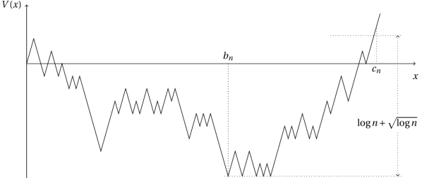
Let $\rho_{x},x\in\mathbb{Z}$ be given by (1) and define the potential $V=\{V(x)\,:\,x\in\mathbb{Z}\}$ by

$$V(x)=\left\{\begin{array}[]{ll}\sum_{y=1}^{x}\log\rho_{y}&\mbox{if $x>0$,}\\ 0&\mbox{if $x=0$,}\\ -\sum_{y=x+1}^{0}\log\rho_{y}&\mbox{if $x<0$.}\end{array}\right.$$ (9)

Then, $V$ is a (double-sided) random walk, an example of a realisation of $V$ can be seen on Figure 1. Setting $C(x,x+1)=\exp[-V(x)]$, for any integer $x$, under quenched law the Markov chain $X$ is an electric network in the sense of Doyle and Snell (1984) or Levin et al. (2009), where $C(x,x+1)$ is the conductance of the (unoriented) bond $(x,x+1)$. In particular, the measure $\mu$ defined as

$$\mu(0)=1,\quad\mu(x)=\exp[-V(x-1)]+\exp[-V(x)],\quad x\in\mathbb{Z}^{*}_{+},$$

is a reversible and invariant measure for the Markov chain $X$. Define the right border $c_{n}$ of the “valley” with depth $\log n+(\log n)^{1/2}$ as the random variable

$$c_{n}=\min\big{\{}x\geq 0\,:\,V(x)-\min_{0\leq y\leq x}V(y)\geq\log n+(\log n)^{1/2}\big{\}},$$ (10)

and the bottom $b_{n}$ of the “valley” as

$$b_{n}=\min\big{\{}x\geq 0\,:\,V(x)=\min_{0\leq y\leq c_{n}}V(y)\big{\}}.$$

On Figure 1, one can see a representation of $b_{n}$ and $c_{n}$. The salient probabilistic feature of a recurrent RWRE is the strong localisation revealed by Sinaĭ (1982). Considered on the spacial scale $\ln^{2}n$ the RWRE becomes localized near $b_{n}.$ We are interested in the shape of the “valley” $(0,b_{n},c_{n})$ when $n$ tends to infinity and we recall the concept of infinite valley introduced by Golosov (1984).

Figure 1: Example of potential derived from a Temkin random environment with parameter $a=0.3$. Simulation with $n=1000$.

Let $\widetilde{V}=\{\widetilde{V}(x)\,:\,x\in\mathbb{Z}\}$ be a collection of random variables distributed as $V$ conditioned to stay positive for any negative $x$, and non-negative for any non negative $x$. Such events having probability zero, a formal definition is using Doob’s $h$-transform (see Golosov (1984)[ Lemma 4], Bertoin (1993)). It has been shown in Golosov (1984), that the finite dimensional distributions of $\{[V(b_{n}+x)-V(b_{n})]\mathrm{1}_{\{-b_{n},\ldots,c_{n}-b_{n}-1\}}(x)\ ;\ x\in\mathbb{Z}\}$ converges to those of $\{\widetilde{V}(x)\,:\,x\in\mathbb{Z}\},$ moreover, (Golosov (1984), pp. 494-495)

$$\sum_{x\in\mathbb{Z}}\exp\left(-\widetilde{V}(x)\right)<\infty.$$ (11)

Besides for the fidi convergence above, it is not true in general that the sequence of the infinite vectors $\{[V(b_{n}+x)-V(b_{n})]\mathrm{1}_{\{-b_{n},\ldots,c_{n}-b_{n}-1\}}(x)\ ;\ x\in\mathbb{Z}\}$ converges in law to $\{\tilde{V}(x),\,x\in\mathbb{Z}\}$. But if we consider instead the sequence of elements of $(\ell^{1},\|\cdot\|_{1})$ given by

$$\Xi_{n}:=\left\{\exp[-(V(b_{n}+x)-V(b_{n}))]\mathrm{1}_{\{-b_{n},\ldots,c_{n}-b_{n}-1\}}(x)\ ;\ x\in\mathbb{Z}\right.\}$$

we can show ( Proposition 4.3) that the sequence of laws $P_{\Xi_{n}}$ of $\Xi_{n}$ is tight, and hence $\Xi_{n}$ converges in distribution to $\ \{\exp[-\widetilde{V}(x)]\ ;\ x\in\mathbb{Z}\}.$ This is done in Theorem (4.4), which is a key auxiliary result for the proof of Theorem (1.1). In the next subsection we formulate this theorem precisely.

1.4 Assumptions and main result

Assumption I.

$\mathbb{E}\log\rho_{0}=0$

We already mentioned that under Assumption (I) for $\mathbb{P}$-almost $\omega$ the Markov chain $X$ is recurrent. We also need to assume

Assumption II.

(i) $\mathbb{P}(\delta_{0}\leq\omega(0)\leq 1-\delta_{0})=1\quad\mbox{for some}\quad\delta_{0}\in(0,1),$

(ii) $\mathbb{V}\mbox{ar}(\log\rho_{0})>0.$

The condition $(i)$ is technical and commonly admitted, whereas $(ii)$ excludes the deterministic case. Moreover, in the proof of Proposition (4.3), Theorem(4.4) and hence in Theorem (1.1) we need to assume the following technical assumption:

Assumption III.

The distribution of $\log\rho_{0}$ is arithmetic, i.e. concentrated on $\{nh;\;n\in\mathbb{Z}\},$ with some $h>0.$

Let $\widetilde{\omega}=\{\widetilde{\omega}(x),\ x\in\mathbb{Z}\}$ be the environment of the walk in the infinite valley:

$$\widetilde{\omega}(x)=\frac{\exp[-\widetilde{V}(x)]}{\exp[-\widetilde{V}(x)]+\exp[-\widetilde{V}(x-1)]},\quad x\in\mathbb{Z}.$$ (12)

Let $\tilde{\nu}$ be a probability measure on $\mathbb{Z}$ defined by

$$\tilde{\nu}(x)=\frac{\exp[-\widetilde{V}(x-1)]+\exp[-\widetilde{V}(x)]}{2\sum_{z\in\mathbb{Z}}\exp[-\widetilde{V}(z)]},\quad x\in\mathbb{Z}.$$ (13)

Thanks to (11) the probability measure (13) is well defined, and is a stationary (and reversible) distribution of a random walk in in the "infinite valley", i.e. the walk governed by the environnement $\tilde{\omega}$.

Define for $n\in\mathbb{N}$ and $x\in\mathbb{Z},$ the local time of the walk in the position $x$:

$$\xi(n,x)=\sum_{k=1}^{n}\mathrm{1}\{X_{k}=x\}\;,$$ (14)

Note that the empirical law (7) of the environment seen from the walker can be expressed using the local time as

$$\mathcal{S}_{n}=\sum_{x\in Z}\frac{\xi(n,x)}{n}\delta_{T_{x}{\omega}}\ \,.$$ (15)

Denote

$$\mathcal{S}_{\infty}:=\sum_{x\in Z}\tilde{\nu}(x)\delta_{T_{x}\widetilde{\omega}}\,.$$ (16)

Let $\Omega:=[0,1]^{\mathbb{Z}}$ be provided with the distance $d(\omega,\omega^{\prime})=\sum_{x\in\mathbb{Z}}2^{-|x|}|\omega(x)-\omega^{\prime}(x)|.$

Theorem 1.1.

Under Assumptions I, II and III, the empirical law of the environment seen from the walker converges in distribution, as $n\rightarrow\infty$:

$$\mathcal{S}_{n}\stackrel{{\scriptstyle\mathcal{L}}}{{\longrightarrow}}\mathcal{S}_{\infty}$$ (17)

in the space ${\mathcal{P}}(\Omega)$ equipped with the topology of the weak convergence of probability measures.

Note that in particular, for every $F:\Omega\rightarrow\mathbb{R}$ continuous and bounded, the "weak" ergodic theorem (8) holds, and therefore for every $m\in\mathbb{N},$ $g:[0,1]^{2m+1}\rightarrow\mathbb{R},$ continuous,

$$\frac{1}{n}\sum_{k=1}^{n}g(\omega(X_{k}-m),\ldots,\omega(X_{k}+m))\stackrel{{\scriptstyle\mathcal{L}}}{{\longrightarrow}}\sum_{x\in\mathbb{Z}}g(\widetilde{\omega}(x-m),\ldots,\widetilde{\omega}(x+m))\tilde{\nu}(x)\;.$$

Again in particular, for every $f:[0,1]\rightarrow\mathbb{R},$ continuous,

$$\frac{1}{n}\sum_{k=1}^{n}f(\omega(X_{k}))\stackrel{{\scriptstyle\mathcal{L}}}{{\longrightarrow}}\sum_{x\in\mathbb{Z}}f(\widetilde{\omega}(x))\tilde{\nu}(x)\;.$$

Denote by ${\mathcal{E}}$ the expectation with respect to the law of $\tilde{V}=(\tilde{V}(x))_{x\in\mathbb{Z}}$ and let us define $\mathbb{Q}\in{\mathcal{P}}(\Omega)$ by

$$\int_{\Omega}Fd\mathbb{Q}={\mathcal{E}}\left[\int_{\Omega}Fd\mathcal{S}_{\infty}\right]=\sum_{x\in\mathbb{Z}}{\mathcal{E}}\big{[}\tilde{\nu}(x)F(T_{x}\widetilde{\omega})\big{]}\;,$$

for bounded $F:\Omega\rightarrow\mathbb{R}$. We can view $\mathbb{Q}$ as the $\mathcal{E}$-expectation of $\mathcal{S}_{\infty}$.

Proposition 1.2.

The probability $\mathbb{Q}$ is invariant and reversible for the Markov chain $(\overline{\omega}_{k},k\geq 0)$ in $\Omega$. The measures $\mathbb{P}$ and $\mathbb{Q}$ are mutually singular.

The invariant probability, which is a limit law in the ballistic case, is absolutely continuous with respect to the law of the environment $\mathbb{P},$ see (Molchanov, 1994, P. 273). The one we find here is the first one to be obtained as a limit in the case of zero velocity, and it is singular with respect to $\mathbb{P}.$

The proof of Theorem (1.1) is partially inspired by the paper Gantert et al. (2010) concerning the convergence of centred local times: $(\frac{\xi(n,b_{n}+x)}{n},\;x\in\mathbb{Z})$ to $(\tilde{\nu}(x)),\;x\in\mathbb{Z}$, but the main ingredient, Proposition (4.2) giving the tightness of $\left\{\exp[-(V(b_{n}+x)-V(b_{n}))]\mathrm{1}_{\{-b_{n},\ldots,c_{n}-b_{n}-1\}}(x)\ ;\ x\in\mathbb{Z}\right\}$ is new. In its turn, one part of the proof of Proposition (4.2) is inspired by the paper of Ritter (1981)on the growth of random walks conditioned to stay positive.

1.5 Structure of the paper

In Section(2) we show how the environment’s method can be deduced from Theorem(1.1). Namely we proove the LLN (Proposition (2.1)) and the mixed CLT(Proposition (2.2)) for sums $\sum_{k=1}^{n}f(\Delta X_{k}).$ Section (3) is focused on the proof of Theorem (1.1). Proposition 1.2 is proven in Section(6). Auxiliary results for the proof of Theorem 1.1, and in particular Proposition (4.2) are proven in Section (4).

2 Examples: environnement’s method

2.1 Law of large numbers for functions of the steps

Proposition 2.1.

Let $f:\{-1;1\}\rightarrow\mathbb{R}.$ Denote $\Delta X_{k}=X_{k+1}-X_{k},$ $k\in\mathbb{N}.$ Then the following convergence in annealed probability holds :

$$\frac{1}{n}\sum_{k=1}^{n}f(\Delta X_{k})\stackrel{{\scriptstyle\mathbf{P}}}{{\longrightarrow}}\frac{f(1)+f(-1)}{2},\quad\quad{n\rightarrow\infty}.$$

In particular, $X_{n}/n\stackrel{{\scriptstyle\mathbf{P}}}{{\longrightarrow}}0,\quad{n\rightarrow\infty}.$

Proof.

Denote

$$\mathcal{F}_{n}=\sigma\{\Delta X_{0},\ldots,\Delta X_{n},\;\omega({X_{0}}),\ldots,\omega({X_{n+1}})\}$$ (18)

and let’s write the martingale difference decomposition :

$$\frac{1}{n}\sum_{k=1}^{n}f(\Delta X_{k})=\frac{1}{n}\sum_{k=1}^{n}\left(f(\Delta X_{k})-\mathbf{E}(f(\Delta X_{k})|\mathcal{F}_{k-1})\right)+\frac{1}{n}\sum_{k=1}^{n}\mathbf{E}(f(\Delta X_{k})|\mathcal{F}_{k-1}).$$ (19)

Then $D_{k}:=f(\Delta X_{k})-\mathbf{E}(f(\Delta X_{k})|\mathcal{F}_{k-1});\,k\in\mathbb{N}$ are centred, uniformly bounded and non-correlated, (the last can be immediately seen for $D_{k}$ and $D_{m}$, $k<m$ by conditioning on $\mathcal{F}_{m-1}).$ Hence

$$\frac{1}{n}\sum_{k=1}^{n}\left(f(\Delta X_{k})-\mathbf{E}(f(\Delta X_{k})|\mathcal{F}_{k-1})\right)\stackrel{{\scriptstyle\mathbb{L}^{2}}}{{\longrightarrow}}0.$$ (20)

Remark that

$$\mathbf{E}(f(\Delta X_{k})|\mathcal{F}_{k-1}))=f(1)\omega({X_{k}})+f(-1)(1-\omega({X_{k}})).$$

Theorem 1.1 gives the following convergence in distribution :

$$\frac{1}{n}\sum_{k=1}^{n}\mathbf{E}(f(\Delta X_{k})|\mathcal{F}_{k-1})\stackrel{{\scriptstyle\mathcal{L}}}{{\longrightarrow}}\sum_{x\in\mathbb{Z}}\left(f(1)\tilde{\omega}(x)+f(-1)(1-\tilde{\omega}(x))\right)\tilde{\nu}(x)=\frac{f(1)+f(-1)}{2}.$$ (21)

Indeed, using the definitions (13) and (12) ,

$$\sum_{x\in\mathbb{Z}}\tilde{\omega}(x)\tilde{\nu}(x)=\sum_{x\in\mathbb{Z}}(1-\tilde{\omega}(x))\tilde{\nu}(x).$$

Using (20) and (21) together in (19) this completes the proof.

∎

Proposition 2.2.

Let $f:\{-1;1\}\rightarrow\mathbb{R}$ and $(\mathcal{F}_{n})$ defined by (18). Then the following mixing CLT holds:

$$\frac{1}{\sqrt{n}}\sum_{k=1}^{n}\left(f(\Delta X_{k})-\mathbf{E}(f(\Delta X_{k})|\mathcal{F}_{k-1})\right)\stackrel{{\scriptstyle\mathcal{L}}}{{\longrightarrow}}Z,$$ (22)

where $Z$ is a random variable with the characteristic function $\phi_{Z}(t)=\mathbf{E}(\exp(-\frac{1}{2}\eta^{2}t^{2}),$ and $\eta$ is a random variable defined by: $\eta^{2}\stackrel{{\scriptstyle\mathcal{L}}}{{=}}(f(1)-f(-1))^{2}\sum_{x\in\mathbb{Z}}\tilde{\omega}(x)(1-\tilde{\omega}(x))\tilde{\nu}(x)$. That is $Z\stackrel{{\scriptstyle\mathcal{L}}}{{=}}\eta U$ where $\eta$ and $U$ are independent and $U\sim{\cal{N}}(0,1).$

Proof.

In this proof we will rely on Theorem 3.4 from Hall and Heyde (1980). Define for $k=1,\ldots,n$

$$D_{nk}:=\frac{1}{\sqrt{n}}\left(f(\Delta X_{k})-\mathbf{E}(f(\Delta X_{k})|\mathcal{F}_{k-1})\right)=\frac{1}{\sqrt{n}}\left(f(\Delta X_{k})-f(1)\omega({X_{k}})-f(-1)(1-\omega({X_{k})})\right).$$

Let $S_{n0}=0,$ $S_{ni}=\sum_{k=1}^{i}D_{nk}$ and put for $i=1,\ldots,n,$ $\mathcal{F}_{ni}:=\mathcal{F}_{i}.$ Then $S_{ni}$ is adapted to $\mathcal{F}_{i}.$ Let $U_{ni}^{2}=\sum_{k=1}^{i}D_{nk}^{2}.$ Denote

$$\mathcal{G}_{n}=\sigma\{\omega({X_{0}}),\ldots,\omega({X_{n+1}})\},$$

Clearly $\mathcal{G}_{n}\subset\mathcal{F}_{n}.$ Let for $i=1,\ldots,n,$

$$\mathcal{G}_{n,i}:=\mathcal{F}_{ni}\vee\mathcal{G}_{n}=\mathcal{F}_{i}\vee\mathcal{G}_{n}=\sigma(\Delta X_{1},\ldots,\Delta X_{i},\omega({X_{0}}),\ldots,\omega({X_{n+1}})\}.$$

Next we have

$$\max_{i=1\ldots n}|D_{ni}|\leq\frac{2\|f\|}{\sqrt{n}}\longrightarrow 0\quad\mbox{ and}\quad\mathbf{E}\left(\max_{i=1\ldots n}|D_{ni}|^{2}\right)\leq\frac{2\|f\|^{2}}{n}.$$ (23)

eq:estimate Define a random sequence $(u_{n}^{2})$ by

$$u_{n}^{2}=\sum_{k=1}^{n}\mathbf{E}\left(D_{nk}^{2}|\mathcal{F}_{k-1}\right).$$

It is easy to see that

$$\mathbf{E}\left(D_{nk}^{2}|\mathcal{F}_{k-1}\right)=\frac{1}{n}(f(1)-f(-1))^{2}\omega({X_{k}})(1-\omega({X_{k}})),$$

hence the sequence $(u_{n}^{2})$ is $(\mathcal{G}_{n})-$ adapted. In order to show the convergence in probability ( the condition of Theorem 3.4 $(3.28)$ from Hall and Heyde (1980)):

$$U_{nn}^{2}-u_{n}^{2}=\sum_{k=1}^{n}\left(D_{nk}^{2}-\mathbf{E}(D_{nk}^{2}|\mathcal{F}_{k-1})\right)\stackrel{{\scriptstyle\mathbb{P}}}{{\longrightarrow}}0,$$ (24)

we remark that $\left(D_{nk}^{2}-\mathbf{E}(D_{nk}^{2}|\mathcal{F}_{k-1})\right);\ k=1,\ldots,n,$ are centred, $(\mathcal{F}_{k})-$ adapted and non correlated. Indeed, if $k<m,$ then $k\leq m-1$ and

$$\mathbf{E}\left[\left(D_{nk}^{2}-\mathbf{E}(D_{nk}^{2}|\mathcal{F}_{k-1})\right)\left(D_{nm}^{2}-\mathbf{E}(D_{nm}^{2}|\mathcal{F}_{m-1})\right)\right]=$$

$$\mathbf{E}\left[\left(D_{nk}^{2}-\mathbf{E}(D_{nk}^{2}|\mathcal{F}_{k-1})\right)\mathbf{E}\left[\left(D_{nm}^{2}-\mathbf{E}(D_{nm}^{2}|\mathcal{F}_{m-1})\right)|\mathcal{F}_{m-1}\right]\right]=0.$$

Hence, using (23), $U_{nn}^{2}-u_{n}^{2}$ converges to $0$ in $\mathbb{L}^{2}$, and hence in probability:

$$\mathbf{E}\left(\sum_{k=1}^{n}\left(D_{nk}^{2}-\mathbf{E}(D_{nk}^{2}|\mathcal{F}_{k-1})\right)\right)^{2}=\sum_{k=1}^{n}\mathbf{E}\left(D_{nk}^{2}-\mathbf{E}(D_{nk}^{2}|\mathcal{F}_{k-1})\right)^{2}\leq\frac{2n\|f\|^{4}}{n^{2}}\rightarrow 0.$$

Then for all $i=1\ldots n,$ $\mathbb{E}\left(D_{ni}|\mathcal{G}_{n,i-1}\right)=0,$ hence the condition $(3.29)$ of Theorem 3.4 from Hall and Heyde (1980) follows.

Applying Theorem (1.1) we see that

$$u_{n}^{2}=(f(1)-f(-1))^{2}\frac{1}{n}\sum_{k=1}^{n}\omega({X_{k}})(1-\omega({X_{k}}))\stackrel{{\scriptstyle\mathcal{L}}}{{\longrightarrow}}(f(1)-f(-1))^{2}\sum_{x\in\mathbb{Z}}\tilde{\omega}(x)(1-\tilde{\omega}(x))\tilde{\nu}(x).$$

Then, using (24),

$$U^{2}_{nn}=(U^{2}_{nn}-u_{n}^{2})+u_{n}^{2}\stackrel{{\scriptstyle\mathcal{L}}}{{\longrightarrow}}\eta^{2}:=(f(1)-f(-1))^{2}\sum_{x\in\mathbb{Z}}\tilde{\omega}(x)(1-\tilde{\omega}(x))\tilde{\nu}(x).$$

and the theorem follows. ∎

3 Proof of Theorem 1.1

Proof.

By definition, claim (17) is equivalent to

$$\lim_{n\rightarrow\infty}{\mathbf{E}}G(\mathcal{S}_{n})={\mathcal{E}}G(\mathcal{S}_{\infty})$$ (25)

for all bounded continuous $G:{\mathcal{P}}(\Omega)\rightarrow\mathbb{R}$. We first observe that it is sufficient to prove (25) for all $G$ of the form

$$G({\mathcal{S}})=\sum_{l=1}^{n}\left(\int_{\Omega}F_{1}d{\mathcal{S}}\times\ldots\times\int_{\Omega}F_{l}d{\mathcal{S}}\right)$$ (26)

with arbitrary integers $n$, $m,$ $l$ and $F_{k}:[0,1]^{2m+1}\rightarrow\mathbb{R}$ continuous ($1\leq k\leq l$). Indeed, let $d$ be a distance on $\Omega$ defined by

$$d(\omega,\omega^{\prime})=\sum_{x\in\mathbb{Z}}\frac{1}{2^{x}}|\omega(x)-\omega^{\prime}(x)|.$$

Then $(\Omega,d)$ is a compact separable metric space and hence $({\mathcal{P}}(\Omega),\rho)$, endowed with the Prohorov metric $\rho$, is a compact separable metric space too. The set ${\mathcal{G}}$ of functions $G$ of the form (26) is an algebra of continuous functions on the compact metric space ${\mathcal{P}}(\Omega)$ which contains constant functions and separates the points. By Stone-Weierstrass Theorem, this set is dense in the space ${\mathcal{C}}({\mathcal{P}}(\Omega);\mathbb{R})$ for the supremum norm, and then it suffices to prove (25) for such $G$’s. This, in turn, is equivalent to prove the convergence in distribution:

$$\left(\int_{\Omega}F_{1}d{\mathcal{S}}_{n},\ldots,\int_{\Omega}F_{l}d{\mathcal{S}}_{n}\right)\stackrel{{\scriptstyle\mathcal{L}}}{{\longrightarrow}}\left(\int_{\Omega}F_{1}d{\mathcal{S}}_{\infty},\ldots,\int_{\Omega}F_{l}d{\mathcal{S}}_{\infty}\right)$$ (27)

as $n\rightarrow\infty$. Indeed, using Cramer-Wold device (27) is equivalent to

$$\forall(t_{1},\ldots t_{l})\in\mathbb{R}^{l},\quad\sum_{i=1}^{l}t_{i}\int_{\Omega}F_{i}d{\mathcal{S}}_{n}\stackrel{{\scriptstyle\mathcal{L}}}{{\longrightarrow}}\sum_{i=1}^{l}t_{i}\int_{\Omega}F_{i}d{\mathcal{S}}_{\infty},$$

and finally, as $\sum_{i=1}^{l}t_{i}F_{i}$ is a continuous function on $\Omega$, depending only on the finite number of coordinates, we only need to prove that

$$\forall m\in\mathbb{N}^{*},\;\forall F\in\mathcal{C}_{b}([0,1]^{2m+1}),\;\quad\quad\int_{\Omega}Fd\mathcal{S}_{n}\stackrel{{\scriptstyle\rm law}}{{\longrightarrow}}\int_{\Omega}Fd{\mathcal{S}}_{\infty}.$$ (28)

Bellow we we give the proof of (28), wich is separated on $3$ main steps.
Step 1:Approximation in probability of $\int_{\Omega}Fd\mathcal{S}_{n}$.
For $F$ as in (28), using (14) and (15) let’s write $\mathcal{S}_{n}(F)$ in the "spatial" form

$$\mathcal{S}_{n}(F)=\sum_{x\in\mathbb{Z}}F(T_{x}\omega)\frac{\xi(n,x)}{n}=\sum_{x\in\mathbb{Z}}F(\omega({-m+x}),\ldots,\omega({m+x}))\frac{\xi(n,x)}{n}.$$ (29)

Fix $n\in\mathbb{N}^{*}$ and denote $\mu_{n}=\mu_{n}^{\omega}$ the random probability measure on $\mathbb{Z}_{+}$

$$\mu_{n}(x):=\left\{\begin{array}[]{ll}\frac{1}{Z_{n}}\left(e^{-V(x)}+e^{-V(x-1)}\right)&\mbox{if $0<x<c_{n}$,}\\ \frac{1}{Z_{n}}&\mbox{if $x=0$,}\\ \frac{1}{Z_{n}}e^{-V(c_{n}-1)}&\mbox{if $x=c_{n}$,}\\ 0&\mbox{if $x\notin\{0,\ldots,c_{n}\},$}\end{array}\right.$$ (30)

where $Z_{n}=2\sum_{x=0}^{c_{n}-1}e^{-V(x)},$ where $c_{n}$ and $V$ are respectively defined by (10) and (9). The point is that the local times $\frac{\xi(n,x)}{n},\,x\in\mathbb{Z}_{+}$ can be approached in probability by the quantities $\mu_{n}(x),\ x\in\mathbb{Z}_{+}$ . This argument was found by Gantert et al. (2010). Here we show that more generally, the additive functional $\mathcal{S}_{n}(F)$ can be approached in probability by $\Sigma_{n}(F)=\int_{\Omega}Fd\Sigma_{n}$ with

$$\Sigma_{n}=\sum_{x\in Z}\mu_{n}(x)\delta_{T_{x}{\omega}}\;.$$ (31)

Namely, Proposition 4.1 states that $\forall\varepsilon>0,$

$$\mathbf{P}\left(\left|\mathcal{S}_{n}(F)-\Sigma_{n}(F)\right|>\varepsilon\right)\rightarrow 0.$$ (32)

Note that $\mathcal{S}_{n}$ depends on the walk and on the environment, whereas $\Sigma_{n}$ depends only on the environment. The next three steps allow to show the convergence in law: $\Sigma_{n}(F)\stackrel{{\scriptstyle\mathcal{L}}}{{\longrightarrow}}\mathcal{S}_{\infty}(F).$
Step 2: Expressing $\Sigma_{n}(F)$ as a continuous function of a weakly convergent sequence.
Note that

$$\Sigma_{n}(F)=\sum_{x\in\mathbb{Z}}F(T_{x}\omega)\mu_{n}(x)=\sum_{x\in\mathbb{Z}}F(T_{b_{n}+x}\omega)\mu_{n}(b_{n}+x).$$

Denote by $\Xi_{n}$ the random element in $\ell^{1}$ given by:

$$\Xi_{n}:=\left\{\exp[-(V(b_{n}+x)-V(b_{n}))]\mathrm{1}_{\{-b_{n},\ldots,c_{n}-b_{n}-1\}}(x)\ ;\ x\in\mathbb{Z}\right.\}.$$

Both $\mu_{n}(b_{n}+x)$ and $\omega(b_{n}+x):\ x=-b_{n},\ldots,c_{n}-b_{n}-1\$ can be expressed in terms of $\Xi_{n}$:

$$\mu_{n}(b_{n}+x)= \frac{\Xi_{n}(x)+\Xi_{n}(x-1)}{2\sum_{y\in\mathbb{Z}}\Xi_{n}(y)},$$ (33)

and

$$\omega(b_{n}+x)= \frac{\Xi_{n}(x)}{\Xi_{n}(x)+\Xi_{n}(x-1)}.$$ (34)

Thus, $\Sigma_{n}(F)=H_{F}(\Xi_{n})$ where $H_{F}:{\ell^{1}}\rightarrow\mathbb{R}$ is continuous. In Theorem 4.4 we show that the distribution of $\Xi_{n}$ converges weakly to that of $\{\exp[-\widetilde{V}(x)]\ ;\ x\in\mathbb{Z}\}$ in this space. Together with the continuity on $\ell_{1}$ of $\Sigma_{n}(F)=H_{F}(\Xi_{n})$ that gives the convergence in law

$$\Sigma_{n}(F)\stackrel{{\scriptstyle\mathcal{L}}}{{\longrightarrow}}\mathcal{S}_{\infty}(F).$$ (35)

Step 3 Conclusion: Using (32) and (35) we conclude that $\mathcal{S}_{n}(F)\stackrel{{\scriptstyle\mathcal{L}}}{{\longrightarrow}}\mathcal{S}_{\infty}(F).$ This ends the proof of Theorem 1.1. ∎

4 Auxiliary results for the Proof of Theorem 1.1

4.1 Approximation in probability

Let $\mu_{n}$ be given by (30). Note that $\mu_{n}$ is a probability measure and that it is invariant for the chain $\tilde{\mathrm{X}}^{n}=(\tilde{X}_{t}^{n})_{,t\in\mathbb{N}}$ with value in $\{0,\ldots,c_{n}\}$ and with transition density given by $\tilde{p}^{\omega,n}:\{0,\ldots,c_{n}\}^{2}\rightarrow[0,1]$ given by:

$$\tilde{p}^{\omega,n}(0,1)=\tilde{p}^{\omega,n}(c_{n},c_{n-1})=1$$

and if $\ x\in\{1,\ldots,c_{n}-1\};$

$$\tilde{p}^{\omega,n}(x,x+1)=\omega_{x}\;,\quad\ \tilde{p}^{\omega,n}(x,x-1)=1-\omega_{x}\;.$$

For $x\in\{0,\ldots,c_{n}\}$ we denote by $\tilde{P}^{\omega,n}_{x}$ the law on $\{0,\ldots,c_{n}\}^{\mathbb{N}}$ of the Markov chain $\tilde{\mathrm{X}}^{n}$ starting from $x$.

Proposition 4.1.

Let $\mathcal{S}_{n}$ given by (15) and $\Sigma_{n}$ by(31). For all $F:[0,1]^{2m+1}\rightarrow\mathbb{R}$ continuous, all $\varepsilon>0$ we have

$$\mathbf{P}\left(\left|\mathcal{S}_{n}(F)-\Sigma_{n}(F)\right|>\varepsilon\right)\rightarrow 0.$$

Proof.

Let $n\in\mathbb{N}^{*}$ and $\omega\in\Omega$ be fixed. Denote $T^{0}=0.$ For $y\in\mathbb{Z}^{+},$ denote

$$T_{y}=T^{1}_{y}:=\inf\{t>0,\ X_{t}=y\}$$

and

$$\forall k>1,\quad T^{k}_{y}:=\inf\{t>T^{k-1}_{y},\ X_{t}=y\}$$

the times of successive visits of $y$ by the walk. Using the recurrence of $\mathrm{X}$,

$$\forall k\in\mathbb{N}^{*},\ \forall y\in\mathbb{Z}^{+},\quad T^{k}_{y}<\infty\quad\mathbf{P}-a.s.$$

Denote $k_{n}$ the number of visits of $b_{n}$ by the walk before the time $n:$

$$k_{n}=\sum_{t=0}^{n}\mathrm{1}_{\{b_{n}\}}(X_{t})$$

and let $\mu_{n}$ be given by (30). The random walk with value in $\{0,\ldots,c_{n}\}$, reflected in $0$ and $c_{n},$ admits $\mu_{n}$ as an invariant measure, and $k_{n}/n$ can be compared with $\mu_{n}$. First of all we obtain a bound on the quenched probability of the deviation of $k_{n}/n$ from $\mu_{n}$.

$$P^{\omega}_{0}\left(\left|\frac{k_{n}}{n}-\mu_{n}(b_{n})\right|>\varepsilon\right)\leq$$ (36)

$$P^{\omega}_{0}\left(\left|\frac{k_{n}}{n}-\mu_{n}(b_{n})\right|>\varepsilon,\ T_{b_{n}}<n\varepsilon/2,\ T_{c_{n}}>n\right)+P^{\omega}_{0}\left(T_{b_{n}}\geq n\varepsilon/2\right)+P^{\omega}_{0}\left(T_{c_{n}}\leq n\right).$$

For the first term of the inequality (36) we can write:

$$P^{\omega}_{0}\left(\left|\frac{k_{n}}{n}-\mu_{n}(b_{n})\right|>\varepsilon,\ T_{b_{n}}<n\varepsilon/2,\ T_{c_{n}}>n\right)\leq P^{\omega}_{0}(B_{1})+P^{\omega}_{0}(B_{2});$$ (37)

Where we have denoted

$$B_{1}:=\left\{{k_{n}}\geq[n(\mu_{n}(b_{n})+\varepsilon)]+1,\ T_{b_{n}}<n\varepsilon/2,\ T_{c_{n}}>n\right\};$$

$$B_{2}:=\left\{{k_{n}}\leq[n(\mu_{n}(b_{n})-\varepsilon)],\ T_{b_{n}}<n\varepsilon/2,\ T_{c_{n}}>n\right\}.$$

Both events $B_{1}$ and $B_{2}$ concern with the part of the trajectory $X_{0},\ldots,X_{n},$ where the value $c_{n}$ did not occurred. Hence $P^{\omega}_{0}(B_{i})=\tilde{P}^{\omega,n}_{0}(B_{i}),\ i=1,2.$ Then, using the definition of $(T^{k}_{b_{n}}),$ strong Markov property and Markov inequality we can write for $n\geq 2/\varepsilon$

$$P^{\omega}_{0}(B_{1})=\tilde{P}^{\omega,n}_{0}(B_{1})\leq\tilde{P}^{\omega}_{0}\left(T^{[n(\mu_{n}(b_{n})+\varepsilon)]+1}_{b_{n}}\leq n\right)\leq\\ \tilde{P}^{\omega,n}_{0}\left(\sum_{k=1}^{[n(\mu_{n}(b_{n})+\varepsilon)]}(T^{k+1}_{b_{n}}-T^{k}_{b_{n}})\leq n\right)\leq\tilde{P}^{\omega,n}_{b_{n}}\left(\sum_{k=1}^{[n(\mu_{n}(b_{n})+\varepsilon)]}\eta_{k}\leq-\frac{n\varepsilon-1}{\mu_{n}(b_{n})}\right)\\ \leq\frac{n(\mu_{n}(b_{n})+\varepsilon)\mu_{n}^{2}(b_{n})\widetilde{\mathbb{V}}\mbox{ar}^{\omega,n}_{b_{n}}\eta_{1}}{(n\varepsilon-1)^{2}}\leq 4\frac{(1+\varepsilon)}{\varepsilon^{2}}\frac{\widetilde{\mathbb{V}}\mbox{ar}^{\omega,n}_{b_{n}}\eta_{1}}{n},$$ (38)

where

$$\eta_{k}=T_{b_{n}}^{k+1}-T_{b_{n}}^{k}-1/\mu_{n}(b_{n})$$

are i.i.d. and centered under $\tilde{P}^{\omega,n}_{b_{n}},$ since $\mu_{n}$ is the invariant probability for $\tilde{p}^{\omega,n}$ and ${\tilde{E}^{\omega,n}_{b_{n}}T_{b_{n}}^{1}=\frac{1}{\mu_{n}(b_{n})}.}$ Similar arguments give

$$P^{\omega}_{0}(B_{2})=\tilde{P}^{\omega,n}_{0}(B_{2})\leq\tilde{P}^{\omega}_{0}\left(T^{[n(\mu_{n}(b_{n})-\varepsilon)]}_{b_{n}}\geq n,\ T_{b_{n}}<n\varepsilon/2\right)\leq\\ \tilde{P}^{\omega,n}_{0}\left(\sum_{k=1}^{[n(\mu_{n}(b_{n})-\varepsilon)]-1}(T^{k+1}_{b_{n}}-T^{k}_{b_{n}})\geq n(1-\varepsilon/2)\right)\leq\tilde{P}^{\omega,n}_{b_{n}}\left(\sum_{k=1}^{[n(\mu_{n}(b_{n})-\varepsilon)]-1}\eta_{k}\geq\frac{n\varepsilon}{2}\right)\\ \leq 4\frac{n(\mu_{n}(b_{n})-\varepsilon)\widetilde{\mathbb{V}}\mbox{ar}^{\omega,n}_{b_{n}}\eta_{1}}{n^{2}\varepsilon^{2}}\leq 4\frac{(1-\varepsilon)}{\varepsilon^{2}}\frac{\widetilde{\mathbb{V}}\mbox{ar}^{\omega,n}_{b_{n}}\eta_{1}}{n}.$$ (39)

Finally, putting together (36), (37), (38) and (39) we get:

$$P^{\omega}_{0}\left(\left|\frac{k_{n}}{n}-\mu_{n}(b_{n})\right|>\varepsilon\right)\leq \frac{8}{\varepsilon^{2}n}{\widetilde{\mathbb{V}}\mbox{ar}^{\omega,n}_{b_{n}}T_{b_{n}}}+P^{\omega}_{0}\left(T_{b_{n}}\geq n\varepsilon/2\right)+P^{\omega}_{0}\left(T_{c_{n}}\leq n\right),$$ (40)

Under the quenched law $\omega$ is fixed. For fixed $\omega\in\Omega$ and $x\in\mathbb{Z}_{+}$ denote

$$F_{\omega}(x):=F(T_{x}\omega),\quad\overline{F}_{\omega}(x):=F_{\omega}(x)-\Sigma_{n}(F)\quad\mbox{and}\quad\tilde{\varepsilon}=\varepsilon/{3\|F\|_{\infty}}.$$

We will first obtain a non-asymptotic bound on the quenched probability of the deviation $\left|\mathcal{S}_{n}(F)-\Sigma_{n}(F)\right|=\left|\frac{1}{n}\sum_{k=0}^{n}F(T_{X_{k}}\omega)-\Sigma_{n}(F)\right|=\left|\frac{1}{n}\sum_{k=0}^{n}F_{\omega}(X_{k})-\Sigma_{n}(F)\right|$:

$$P^{\omega}_{0}\left(\left|\frac{1}{n}\sum_{k=0}^{n}F_{\omega}(X_{k})-\Sigma_{n}(F)\right|>\varepsilon\right)\leq P^{\omega}_{0}\left(\left|\frac{k_{n}}{n}-\mu_{n}(b_{n})\right|>\varepsilon\right)+P^{\omega}_{0}\left(T_{c_{n}}<n\right)+$$

$$P^{\omega}_{0}\left(\sum_{k=0}^{T^{1}_{b_{n}}-1}|\overline{F}_{\omega}(X_{k})|>n\varepsilon/3\ \right)+P^{\omega}_{0}\left(\left|\sum_{k=T_{b_{n}}}^{T_{b_{n}}^{k_{n}}-1}\overline{F}_{\omega}(X_{k})\right|>n\varepsilon/3,\ \left|\frac{k_{n}}{n}-\mu_{n}(b_{n})\right|\leq\varepsilon,\ T_{c_{n}}>n\right)+$$

$$P^{\omega}_{0}\left(\sum_{k=T_{b_{n}}^{k_{n}}}^{n}|\overline{F}_{\omega}(X_{k})|>n\varepsilon/3,\ T_{c_{n}}>n\right)$$ (41)

Using the definition of $\tilde{\varepsilon}$ we see that

$$P^{\omega}_{0}\left(\sum_{k=0}^{T^{1}_{b_{n}}-1}|\overline{F}_{\omega}(X_{k})|>n\varepsilon/3\right)\leq P^{\omega}_{0}\left(T_{b_{n}}>\tilde{\varepsilon}n\right).$$ (42)

The law of ${T_{b_{n}}^{k_{n}+1}}-{T_{b_{n}}^{k_{n}}}$ conditionaly on $\mathcal{F}_{T_{b_{n}}^{k_{n}}}$ is that of $T_{b_{n}}.$ Also, using the definition (30) we can see that $\mu_{n}(b_{n})\geq 1/2c_{n}.$ Hence,

$$P^{\omega}_{0}\left(\sum_{k=T_{b_{n}}^{k_{n}}}^{n}|\overline{F}_{\omega}(X_{k})|>n\varepsilon/3,\ T_{c_{n}}>n\right)=\tilde{P}^{\omega}_{0}\left(\sum_{k=T_{b_{n}}^{k_{n}}}^{n}|\overline{F}_{\omega}(X_{k})|>n\varepsilon/3,\ T_{c_{n}}>n\right)\leq$$

$$\tilde{P}^{\omega}_{0}\left(\sum_{k=T_{b_{n}}^{k_{n}}}^{T_{b_{n}}^{k_{n}+1}}|\overline{F}_{\omega}(X_{k})|>n\varepsilon/3\right)\leq\tilde{P}^{\omega,n}_{b_{n}}\left(T_{b_{n}}>n\tilde{\varepsilon}\right)\leq\frac{1}{n\mu_{n}(b_{n})\tilde{\varepsilon}}\leq\frac{2c_{n}}{n\tilde{\varepsilon}}.$$ (43)

Now we obtain a bound for the main term of the decomposition (4.1). Denote for $k\in\mathbb{N}^{*},$

$$\xi_{k}:=\sum_{l=T_{b_{n}}^{k}}^{T_{b_{n}}^{k+1}-1}\overline{F}_{\omega}(X_{l}).$$

Under $\tilde{P}^{\omega,n}_{0}$ the random variables $\ \xi_{k},k\in\mathbb{N}^{*}$ are i.i.d. Their law is that of $\sum_{l=0}^{T_{b_{n}}-1}\overline{F}_{\omega}(X_{l})$ under $\tilde{P}^{\omega,n}_{b_{n}}$ and they are centered, because

$$E^{\omega,n}_{b_{n}}\sum_{l=0}^{T_{b_{n}}-1}F_{\omega}(X_{l})=\mu_{n}(F_{\omega}(\cdot))E^{\omega,n}_{b_{n}}T_{b_{n}}=\Sigma_{n}(F)E^{\omega,n}_{b_{n}}T_{b_{n}}.$$

Hence $M_{m}:=\sum_{k=1}^{m}\xi_{k};\ m\in\mathbb{N}^{*}$ is a square-integrable martingale under $\tilde{P}^{\omega,n}_{0}$. Using Kolmogorov inequality we get:

$$P^{\omega}_{0}\left(\left|\sum_{k=T_{b_{n}}}^{T_{b_{n}}^{k_{n}+1}-1}\overline{F}_{\omega}(X_{k}))\right|>n\varepsilon/3,\ \left|\frac{k_{n}}{n}-\mu_{n}(b_{n})\right|\leq\varepsilon,\ T_{b_{n}}<\varepsilon n,\ T_{c_{n}}>n\right)\leq$$ (44)

$$\tilde{P}^{\omega,n}_{0}\left(\left|\sum_{k=1}^{k_{n}}\xi_{k}\right|>n\varepsilon/3,\ \left|\frac{k_{n}}{n}-\mu_{n}(b_{n})\right|\leq\varepsilon\right)\leq$$

$$\tilde{P}^{\omega,n}_{0}\left(\sup_{m=1,\ldots[n(\mu_{n}(b_{n})+\varepsilon)]}\left|\sum_{k=1}^{m}\xi_{k}\right|>n\varepsilon/3\right)\leq\frac{9(\mu_{n}(b_{n})+\varepsilon)\widetilde{\mathbb{V}}\mbox{ar}_{b_{n}}^{\omega,n}(\xi_{1})}{n\varepsilon^{2}}$$

Pluging in (4.1) the bounds (40), (42), (4.1) and (44) we obtain:

$$P^{\omega}_{0}\left(\left|\mathcal{S}_{n}(F)-\Sigma_{n}(F)\right|>\varepsilon\right)\leq\\ P^{\omega}_{0}\left(T_{b_{n}}\geq n\varepsilon/2\right)+P^{\omega}_{0}\left(T_{b_{n}}\geq n\tilde{\varepsilon}\right)+2P^{\omega}_{0}\left(T_{c_{n}}\leq n\right)+\\ \frac{8}{n\varepsilon^{2}}{\widetilde{\mathbb{V}}\mbox{ar}^{\omega,n}_{b_{n}}T_{b_{n}}}+\frac{9(1+\varepsilon)\widetilde{\mathbb{V}}\mbox{ar}_{b_{n}}^{\omega,n}(\xi_{1})}{n\varepsilon^{2}}+\frac{2c_{n}}{n\tilde{\varepsilon}}.$$ (45)

To conclude the proof we need to estimate $\widetilde{\mathbb{V}}\mbox{ar}^{\omega,n}_{b_{n}}(\xi_{1}).$ For $x\in Z_{+}$ introduce

$$Y_{x}=\sum_{j=0}^{T_{b_{n}}}\mathrm{1}_{\{x\}}(X_{j})$$

the local time in $x$ during $1$-th excursion from $b_{n}$ to $b_{n}.$ Note that under $\tilde{P}^{n}_{b_{n}},$

$$\xi_{1}=\sum_{x=0,\ldots,c_{n}}\overline{F}_{\omega}(x)Y_{x}$$ (46)

and

$$\widetilde{\mathbb{V}}\mbox{ar}^{\omega,n}_{b_{n}}(\xi_{1})\leq(c_{n}+1)\|\overline{F}_{\omega}\|_{\infty}^{2}\sum_{x=0,\ldots,c_{n}}\widetilde{\mathbb{V}}\mbox{ar}^{\omega,n}_{b_{n}}(Y_{x}).$$

Taking $\overline{F}_{\omega}=1$ in (46) we get:

$$\widetilde{\mathbb{V}}\mbox{ar}^{\omega,n}_{b_{n}}(T_{b_{n}})\leq(c_{n}+1)\sum_{x=0,\ldots,c_{n}}\widetilde{\mathbb{V}}\mbox{ar}^{\omega,n}_{b_{n}}(Y_{x}).$$

Using Lemma (7.1), which is given in Appendix, for all $\eta>0,$ there exists $\delta>0$ and an event $\Omega_{\eta,\delta}\subset\Omega$ with $\mathbb{P}(\Omega_{\eta,\delta})>1-\eta$ such that : $\forall\omega\in\Omega_{\eta,\delta},\forall x\in[0,c_{n}],$

$$\qquad\widetilde{\mathbb{V}}\mbox{ar}^{\omega,n}_{b_{n}}(Y_{x})\leq n^{1-\delta}\;.$$

The proof of Lemma 7.1 is given in appendix. As a consequence, for all $\eta>0,$ there exists $1>\delta>0,$ and a set $\Omega_{\eta,\delta}$ with $\mathbb{P}(\Omega_{\eta,\delta})>1-\eta,$ such that for all $\omega\in\Omega_{\eta,\delta}$ it holds

$$P^{\omega}_{0}\left(\left|\mathcal{S}_{n}(F)-\Sigma_{n}(F)\right|>\varepsilon\right)\leq C\frac{c_{n}^{2}n^{1-\delta}}{n}+2P^{\omega}_{0}\left(T_{b_{n}}\geq(\varepsilon+\tilde{\varepsilon})n\right)+2P^{\omega}_{0}\left(T_{c_{n}}\leq n\right).$$ (47)

The last bound tends to zero. Indeed, from Golosov (1984), Lemma 1, ${P^{\omega}_{0}\left({T_{b_{n}}}>n\varepsilon^{\prime}\right)\rightarrow 0}$ for all $\omega\in\Omega$ and $\varepsilon^{\prime}>0.$ And from Golosov (1984), Lemma 7, for all $\omega\in\Omega,$ ${P^{\omega}_{0}\left(T(c_{n})\leq n\right)\rightarrow 0}.$ ∎

4.2 Convergence in distribution of $\Xi_{n}$

Recall that $\Xi_{n}$ is a random element with values in $\ell^{1}$ given by

$$\Xi_{n}:=\left\{\exp[-(V(b_{n}+x)-V(b_{n}))]\mathrm{1}_{\{-b_{n},\ldots,c_{n}-b_{n}-1\}}(x)\ ;\ x\in\mathbb{Z}\right.\}$$

Denote by $P_{\Xi_{n}}$ the law of $\Xi_{n}$ on $(\ell^{1},\mathcal{B}(\ell^{1})).$ The following proposition is the key technical result of the paper.

Proposition 4.2.

Suppose that Assumptions (I) and(II) are satisfied. Then the following holds:

i) For all $\eta\in]0,1/2[$ and $\delta>0$,

$$\lim_{K\rightarrow+\infty}\liminf_{n\rightarrow\infty}\mathbb{P}\left(V(b_{n}+x)-V(b_{n})\geq\delta x^{\eta},\ \forall x\in\llbracket K,c_{n}-b_{n}\rrbracket\ \ \right)=1.$$

ii) Suppose that in addition that Assumptions (III) is satisfied. Then for all $\eta\in]0;1/3[$,

$$\lim_{K\rightarrow+\infty}\liminf_{n\rightarrow\infty}\mathbb{P}\left(V(b_{n}-x)-V(b_{n})\geq x^{\eta},\ \forall x\in\llbracket K,b_{n}\rrbracket\ \ \right)=1.$$

The proposition (4.2) is proven in Section (5).

Proposition 4.3.

Suppose that Assumptions (I),(II) and (III) are satisfied. Then the sequence $P_{\Xi_{n}}$ is relatively compact in $(\ell^{1},\|\cdot\|_{1})$.

Proof.

Recall that $(\ell^{1},\|.\|_{1})$ is a complete separable metric space and hence , using Prohorov’s theorem (Billingsley (1999)), the sequence of distributions $P_{\Xi_{n}}$ is relatively compact if and only if it is tight. Recall also the characterization of the compacts in $(\ell^{1},\|.\|_{1}):$

$$\mathcal{K}\subset\ell^{1}\quad\mbox{is compact}\quad\Longleftrightarrow\quad\sup_{l\in\mathcal{K}}\|l\|_{1}<\infty\quad\mbox{and}\quad\lim_{N\rightarrow\infty}\sup_{l\in\mathcal{K}}\sum_{|x|\geq N}|l_{x}|=0.$$

Let $\eta\in(0,1/3),$ $K>0,$ and denote

$$\mathcal{K}(\eta,K):=\{l\in\ell^{1};\;|l_{x}|\leq 1\quad\mbox{and}\quad\forall x\in\mathbb{Z}\quad|l_{x}|\leq e^{-|x|^{\eta}}\quad\mbox{if}\quad|x|\geq K\}.$$

Since $\sum_{x\in\mathbb{Z}}e^{-|x|^{\eta}}<\infty,\$ $\mathcal{K}(\eta,K)\$ is a compact in $\ell^{1}.$ As a consequence of Proposition 4.2, for any fixed $\eta\in(0,1/3),$ forall $\varepsilon>0$, there exists $K>0,$ such that

$$\liminf_{n}\mathbb{P}\left(e^{-(V(b_{n}+x)-V(b_{n}))}<e^{-|x|^{\eta}},\ \forall x\in\llbracket-b_{n},c_{n}-b_{n}\rrbracket;\quad|x-b_{n}|>K\ \right)\geq 1-\varepsilon.$$

Hence, for $n$ large enough $\mathbb{P}(\Xi_{n}\in\mathcal{K}({\eta,K)})\geq 1-\varepsilon$ and the sequence $P_{\Xi_{n}}$ is tight. ∎

Theorem 4.4.

Suppose that Assumptions (I),(II) and (III) are satisfied. Then the sequence $P_{\Xi_{n}}$ converges weakly to the law of $\ \{\exp[-\widetilde{V}(x)]\ ;\ x\in\mathbb{Z}\}$ on $(\ell^{1},\mathcal{B}(\ell^{1}))$.

Proof.

From Golosov (1984) the following convergence of finite dimensional distributions (fidi) holds:

$$\big{\{}\exp[-(V(b_{n}+x)-V(b_{n}))]\ ;\ x\in\mathbb{Z}\big{\}}\stackrel{{\scriptstyle\rm fidi}}{{\longrightarrow}}\big{\{}\exp[-\widetilde{V}(x)]\ ;\ x\in\mathbb{Z}\big{\}}.$$

Using $b_{n}\rightarrow\infty$ a.s. and $c_{n}-b_{n}\rightarrow\infty$ a.s., the finite dimensional distributions of $\Xi_{n}$ converge weakly to those of $\ \{\exp[-\widetilde{V}(x)]\ ;\ x\in\mathbb{Z}\}$ . Denote by $\mathcal{M}$ the class of continuous, bounded, finite-dimensional functions:

$$\mathcal{M}:=\bigcup_{k\in\mathbb{N}^{*}}\big{\{}f\in\mathcal{C}_{b}(\ell^{1}):f(l_{i})=f(l_{i}^{\prime})\;\forall i\in\llbracket-k,k\rrbracket\implies f(l)=f(l^{\prime})\big{\}}.$$

It is clear that $\mathcal{M}$ separates points: if $l\in\ell^{1},$ $l^{\prime}\in\ell^{1},$ $l\neq l^{\prime},$ that there exists $f\in\mathcal{M},$ such that $f(l)\neq f(l^{\prime}).$ Since $(\ell^{1},d)$ is separable and complete, and $\mathcal{M}$ separates points, using Theorem 4.5 from Stewart N. Ethier (2005) $\mathcal{M}$ is separating. Now the claim follows directly from proposition (4.3) and lemma 4.3 of Stewart N. Ethier (2005).

∎

5 Proof of Proposition (4.2)

Proof.

We start by proving $ii).$ Let $T_{0}:=0$ and for all $\ell\in\mathbb{N}^{*},$ put

$$\ T_{\ell+1}:=\inf\{y>T_{\ell},\ V(y)<V(T_{\ell})\}.$$

The sequence $(T_{\ell})_{\ell\in\mathbb{N}}$ is the sequence of the strict descending ladder epochs of $V.$ Let

$$e_{\ell}=((V(z)-V(T_{\ell-1})),\;T_{\ell-1}\leq z<{T_{\ell}}),\quad\ell\in\mathbb{N}^{*}.$$

Using the strong Markov property of $V,$ the sequence $(e_{\ell});\;\ell\in\mathbb{N}^{*}$ is an i.i.d. sequence. Let $N(n)$ be a random time, such that $b_{n}=T_{N(n)}.$ Namely, setting as previously $L_{n}:=\ln n+\sqrt{\ln n},$ we have following Golosov (1984) p.492,

$$N(n):=\inf\{\ell\in\mathbb{N}^{*};\;\max\{V(z)-V(T_{\ell-1});\;T_{\ell-1}\leq z<T_{\ell}\}\geq L_{n}\}.$$

Due to the independence and the equidistribution of the excursions $(e_{\ell});\;\ell\in\mathbb{N}^{*},$ the random variable $N(n)$ is geometrically distributed with the parameter

$$p_{n}:=\mathbb{P}(\tau_{L_{n}}<\tau_{0-}),\;\;\mbox{where}$$ (48)

$$\tau_{L_{n}}:=\inf\{z>0,\;V(z)\geq L_{n}\}\quad\mbox{and}\quad\tau_{0-}:=\inf\{z>0;\;V(z)<0\}.$$

Let $K\in\mathbb{N}^{*}$ and denote

$$C(\eta,K,n): =\{\forall x=K,\ldots,b_{n},\;\ V(b_{n}-x)-V(b_{n})\geq x^{\eta}\}$$

$$=\{\forall y=0,\ldots,b_{n}-K,\;V(y)-V(b_{n})\geq|y-b_{n}|^{\eta}\}.$$

Keeping in mind the relation $b_{n}=T_{N(n)},$ we can observe that

$$C(\eta,K,n)=\{\forall\ell=0,\ldots N(n)-1;\ |T_{\ell}-T_{N(n)}|\geq K;\ V(T_{\ell})-V(T_{N(n)})\geq|T_{\ell}-T_{N(n)}|^{\eta}\}$$ (49)

Indeed, let $\ell(y)\in\mathbb{N}$ be the number of ladder excursion containing $y$, i.e. $T_{\ell(y)}\leq y<T_{\ell(y)+1}$, then using the fact that the function $x\rightarrow x^{\eta}$ is increasing on $\mathbb{R}_{+},$ $V(y)\geq V(T_{\ell(y)})$ and $V(T_{\ell})-V(T_{N(n)})\geq|T_{\ell}-T_{N(n)}|^{\eta}$ for all $\ell\in\mathbb{N},$ we have

$$V(y)-V(T_{N(n)})=V(y)-V(T_{\ell(y)})+V(T_{\ell(y)})-V(T_{N(n)})\geq|T_{\ell(y)}-T_{N(n)}|^{\eta}\geq|y-T_{N(n)}|^{\eta}.$$

Which prove (49).

Due to the arithmeticity of the law of $\log\rho_{0},$ for all $\ell\in\mathbb{N},$ $V(T_{\ell})-V(T_{\ell+1})\geq h.$ Therefore we can write:

$$\mathbb{P}(C^{c}(\eta,K,n))=$$ (50)

$$\sum_{N=1}^{\infty}\mathbb{P}(\exists\ell=0,\ldots,N-1,\ T_{N}-T_{\ell}\geq K,\;V(T_{\ell})-V(T_{N})<|T_{\ell}-T_{N}|^{\eta};\ N(n)=N)\leq$$

$$\sum_{N=1}^{M}\mathbb{P}(N(n)=N)+\sum_{N=M+1}^{\infty}\mathbb{P}(\exists m=1,\ldots,M,\ T_{N}-T_{N-m}\geq K;\ N(n)=N)+$$

$$\sum_{N=M+1}^{\infty}\mathbb{P}(\exists m=M+1,\ldots,N,\ T_{N}-T_{N-m}\geq(hm)^{1/\eta};\ N(n)=N):=$$

$$S_{1}(n,M)+S_{2}(K,n,M)+S_{3}(\eta,n,M).$$

Here in the third line we denoted $m=N-\ell$ the number of "ladder" between $T_{N}$ and $T_{\ell}$ and the auxiliary $M\in\mathbb{N}^{*}$ will be choose later. We obviously have

$$S_{1}(n,M)=\sum_{N=1}^{M}(1-p_{n})^{N-1}p_{n}=1-(1-p_{n})^{M}\sim Mp_{n}\rightarrow 0\quad\mbox{if}\quad n\rightarrow\infty.$$ (51)

For the second sum we can write, denoting $\sigma_{\ell}:=T_{\ell}-T_{\ell-1}$ the length of the $\ell$-th ladder

$$S_{2}(K,n,M):=\sum_{N=M+1}^{\infty}\mathbb{P}(\exists m=1,\ldots,M,\ T_{N}-T_{N-m}\geq K;\ N(n)=N)\leq$$

$$\sum_{N=M+1}^{\infty}\mathbb{P}(T_{N}-T_{N-M}\geq K;\;N(n)=N)=\sum_{N=M+1}^{\infty}\mathbb{P}(\sigma_{N-M+1}+\ldots+\sigma_{N}\geq K;\;N(n)=N)\leq$$

$$\sum_{N=M+1}^{\infty}\sum_{\ell=N-M+1}^{N}\mathbb{P}(\sigma_{\ell}\geq K/M;\;N(n)=N).$$

The event $\{N(n)=N\}$ can be written as

$$\{N(n)=N\}=\{\tau^{1}_{0-}<\tau^{1}_{L_{n}};\ldots;\tau^{N-1}_{0-}<\tau^{N-1}_{L_{n}};\tau^{N}_{0-}>\tau^{N}_{L_{n}}\},$$

where we denoted $\tau^{\ell}_{0-}:=\tau_{0-}\circ\theta_{T_{\ell}}$ and $\tau^{\ell}_{L_{n}}:=\tau_{L_{n}}\circ\theta_{T_{\ell}}.$ Let $c_{Sp}>0$ be such that $\forall a>c_{Sp},$ $\mathbb{P}(\tau_{0-}>a)\leq{C}{a^{-1/2}},$ where $C$ is a positive constant. Following Spitzer (1960) we can choose such a constant $c_{Sp}$. Let $M$ in (50) be fixed in a such a way that $K/M>c_{Sp}$. Then, using the independence of the ladder excursions, together with the definition 48, we can write (note that $\sigma_{1}=\tau^{1}=\tau_{0-}$),

$$\mathbb{P}(\sigma_{\ell}\geq\frac{K}{M};\;N(n)=N)\leq\mathbb{P}(\sigma_{\ell}\geq\frac{K}{M}\cap\tau^{\ell}_{0-}<\tau^{\ell}_{L_{n}})p_{n}(1-p_{n})^{N-2}\leq C\sqrt{\frac{M}{K}}p_{n}(1-p_{n})^{N-2}.$$

Using this bound we see that

$$S_{2}(K,n,M)\leq\sum_{N=M+1}^{\infty}\frac{C(M_{1})^{3/2}p_{n}(1-p_{n})^{N-2}}{\sqrt{K}}=\frac{C(M_{1})^{3/2}(1-p_{n})^{M-1}}{\sqrt{K}}\leq\frac{C(M_{1})^{3/2}}{\sqrt{K}}.$$ (52)

To find a bound for $S_{3}(\eta,n,M)$ we introduce

$$B_{m}:=\{T_{N}-T_{N-m}\geq(hm)^{1/\eta},\;\;T_{N}-T_{N-(m-1)}<(h(m-1))^{1/\eta}\}.$$

Then

$$S_{3}(\eta,n,M)=$$ (53)

$$\sum_{N=M+1}^{\infty}\mathbb{P}(\exists m=M+1,\ldots,N,\ T_{N}-T_{N-m}\geq(V(T_{N-m})-V(T_{n}))^{1/\eta};\ N(n)=N)\leq$$

$$\sum_{N=M+1}^{\infty}\mathbb{P}(\exists m=M+1,\ldots,N,\ T_{N}-T_{N-m}\geq(hm)^{1/\eta};\ N(n)=N)\leq$$

$$\sum_{N=M+1}^{\infty}\sum_{m=M+1}^{N}\mathbb{P}(B_{m}\cap N(n)=N)$$

Remark that $T_{N}-T_{N-m}=T_{N}-T_{N-m+1}+\sigma_{N-m}$ and hence $B_{m}\subset\{\sigma_{N-m}\geq c^{\prime\prime}m^{\frac{1}{\eta}-1}\}$ for $c=\eta^{-1}\sup_{[1;2]}x^{1/\eta-1}\leq\eta^{-1}2^{1/\eta-1}.$ Chose $M$ such that $c^{\prime\prime}M^{\frac{1}{\eta}-1}>c_{Sp}$ where $c_{Sp}$ is again a constant of Spitzer. Then we can write

$$\sum_{m=M+1}^{N}\mathbb{P}(B_{m}\cap N(n)=N)\leq\sum_{m=M+1}^{N}\mathbb{P}(\sigma_{N-m}\geq c^{\prime\prime}m^{\frac{1}{\eta}-1};\tau^{m}_{0-}<\tau^{m}_{L_{n}})p_{n}(1-p_{n})^{N-2}\\ \leq p_{n}(1-p_{n})^{N-2}\sum_{m=M+1}^{N}\mathbb{P}(\sigma_{N-m}\geq c^{\prime\prime}m^{\frac{1}{\eta}-1})=p_{n}(1-p_{n})^{N-2}\sum_{m=M+1}^{N}\mathbb{P}(\tau_{0-}\geq c^{\prime\prime}m^{\frac{1}{\eta}-1})\\ \leq p_{n}(1-p_{n})^{N-2}\sum_{m=M_{1}}^{N}\frac{C}{m^{\frac{(1-\eta)}{2\eta}}}\leq Cp_{n}(1-p_{n})^{N-2}M^{3/2-\frac{1}{2\eta}}$$ (54)

Finally we get

$$S_{3}(n)\leq\sum_{N=M}^{\infty}p_{n}(1-p_{n})^{N-2}M^{3/2-\frac{1}{2\eta}}\leq M^{3/2-\frac{1}{2\eta}}.$$ (55)

And finally putting together (51), (52) and (55) we obtain from (50):

$$\mathbb{P}(C^{c}(\eta,K,n))=$$ (56)

$$S_{1}(n,M)+S_{2}(K,n,M)+S_{3}(\eta,n,M)\leq Mp_{n}+\frac{M^{3/2}}{\sqrt{K}}+M^{3/2-\frac{1}{2\eta}}.$$

If $\eta<1/3,$ then $3/2-\frac{1}{2\eta}<0.$ Remember that the bound on $S_{2}$ is valuable if $K/M>c_{Sp}$ and that on $S_{3}$, if $c"M^{\frac{1-\eta}{\eta}}>c_{Sp}.$ Hence we first choose $M$ large enough, such that simultaneously $c"M^{\frac{1-\eta}{\eta}}>c_{Sp}$ and $M^{3/2-\frac{1}{2\eta}}\leq\varepsilon.$ Then we get

$$\lim_{K\rightarrow\infty}\limsup_{n\rightarrow\infty}\mathbb{P}(C^{c}(\eta,K,n))\leq\varepsilon$$

which, sins $\varepsilon>0$ is arbitrary, concludes the proof.

Now we prove $i)$.
Recall $V(x)=\sum_{y=1}^{x}\log\rho_{y}$ if $x>0$, $(\log\rho_{y})_{y\in\mathbb{Z}}$ i.i.d. centered. Denote

$$\tau_{\ln}=\inf\big{\{}x\in\mathbb{Z}_{+},\ V(x)\geq\log n+\sqrt{\log n}\big{\}}\;,\quad\tau_{0-}=\inf\big{\{}x\in\mathbb{Z}_{+},\ V(x)<0\big{\}}\;.$$

Using strong Markov property,

$$\mathcal{L}(\{V(b_{n}+x)-V(b_{n}),\ x=K-b_{n},\ldots,c_{n}-b_{n}\})=\mathcal{L}(\{V(x),\ x=K,\ldots,\tau_{\ln}|\tau_{\ln}<\tau_{0-}\})\;.$$

Hence we have to prove

$$\lim_{K\rightarrow+\infty}\inf_{n}\mathbb{P}\left(V(x)\geq\delta x^{\eta},\ \forall x=K,\ldots,\tau_{\ln}\wedge\tau_{0-}\ |\tau_{\ln}<\tau_{0-}\right)=1.$$ (57)

or equivalently

$$\lim_{K\rightarrow+\infty}\sup_{n}\frac{\mathbb{P}\left(\exists x\geq K,\ x<\tau_{\ln}\wedge\tau_{0-},\ V(x)<\delta x^{\eta},\ \tau_{\ln}<\tau_{0-}\right)}{\mathbb{P}\left(\tau_{\ln}<\tau_{0-}\right)}=0.$$ (58)

The following proof is inspired by Ritter (1981). Let $c>1$ be an integer such that $\forall a>c,$ $\mathbb{P}(\tau_{0-}>a)\leq{C}{a^{-1/2}},$ where $C$ is a positive constant. Following Spitzer Spitzer (1960) we can choose such a constant $c$. For $r\in\mathbb{N}^{*},$ denote ${\cal C}_{r}$ the following event

$${\cal C}_{r}:=\{\exists x\in[c^{r-1},c^{r}[;\;\;x<\tau_{\ln}\wedge\tau_{0-};\;\;V(x)<\delta x^{\eta};\;\;\tau_{\ln}<\tau_{0-}\}$$

and denote for $x\in[c^{r-1},c^{r}[$

$${\cal A}_{x}:=\{\forall z\in[c^{r-1},x[;\;\;V_{z}\geq\delta z^{\eta};\;\;V(x)<\delta x^{\eta};\;\;x<\tau_{n}\wedge\tau_{0-}\}$$

Note that ${\cal A}_{x}$ are disjoint for $x\in[c^{r-1},c^{r}[$ and that

$${\cal C}_{r}:=\bigcup_{x=c^{r-1}}^{c^{r}-1}\left\{{\cal A}_{x}\cap\{\tau_{\ln}<\tau_{0-}\}\right\}.$$

For all $x\in\mathbb{N},$ denote $\mathbb{P}:=\mathbb{P}_{0},$ $\mathcal{F}_{x}=\sigma\{V_{0},\ldots,V_{x}\}$. Denote $L_{n}=\log n+\sqrt{\log n}.$ It is easy to see that

$$\forall 0\leq y<L_{n},\quad\mathbb{P}_{y}(\tau_{\ln}<\tau_{0-})\leq\frac{y+c_{0}}{L_{n}}$$

for some positive constant $c_{0}=\sup_{n,y\geq 0}\mathbb{E}_{y}(-V(\tau_{0-})\mid\tau_{0-}<\tau_{\ln})$. Indeed, using Doob stopping theorem, and the fact that $V_{\tau_{L}}>L,$

$$\mathbb{P}_{y}(\tau_{\ln}<\tau_{0-})=\frac{y-\mathbb{E}_{y}[V_{\tau_{0-}}\mid\tau_{0-}<\tau_{\ln}]}{\mathbb{E}_{y}[V_{\tau_{L}}\mid\tau_{L}<\tau_{0-}]-\mathbb{E}_{y}[V_{\tau_{0-}}\mid\tau_{0-}<\tau_{\ln}]}.$$

Since the event $\{\tau_{\ln}<\tau_{0-}\}$ is invariant under shift, using Markov property we can write:

$$\mathbb{P}_{0}\left({\cal A}_{x}\cap\{\tau_{\ln}<\tau_{0-}\}\right)=\mathbb{E}_{0}\left[\mathbb{P}_{0}\left({\cal A}_{x}\cap\{\tau_{\ln}<\tau_{0-}\}|\mathcal{F}_{x}\right)\right]=\\ \mathbb{E}_{0}\left(\forall z\in[c^{r-1},x[;\;\;V_{z}\geq\delta z^{\eta};\;\;V(x)<\delta x^{\eta};\;\;x<\tau_{\ln}\wedge\tau_{0-};\;\;\mathbb{P}_{V_{x}}(\tau_{\ln}<\tau_{0-})\right)\leq\\ \mathbb{P}_{0}\left(\forall z\in[c^{r-1},x[;\;\;V_{z}\geq\delta z^{\eta};\;\;V(x)<\delta x^{\eta};\;\;x<\tau_{\ln}\wedge\tau_{0-}\right){(\delta x^{\eta}+c_{0})}(L_{n})^{-1}=\\ \mathbb{P}({\cal A}_{x}){(\delta x^{\eta}+c_{0})}(L_{n})^{-1}.$$

Hence, using the fact that ${\cal A}_{x}$ are disjoint and that

$$\forall x=c^{r-1},\ldots,c^{r}-1;\quad{\cal A}_{x}\subset\{\tau_{0-}>x\}\subset\{\tau_{0-}>c^{r-1}\},$$

with our choice of $c$, we have

$$\mathbb{P}({\cal C}_{r})=\sum_{x=c^{r-1}}^{c^{r}-1}\mathbb{P}\left({\cal A}_{x}\cap\{\tau_{\ln}<\tau_{0-}\}\right)\leq\frac{\delta c^{r\eta}+c_{0}}{L_{n}}\sum_{x=c^{r-1}}^{c^{r}-1}\mathbb{P}\left({\cal A}_{x}\right)=\\ \frac{\delta c^{r\eta}+c_{0}}{L_{n}}\mathbb{P}\left(\bigcup_{x=c^{r-1}}^{c^{r}-1}{\cal A}_{x}\right)\leq\frac{\delta c^{r\eta}+c_{0}}{L_{n}}\mathbb{P}\left(\tau_{0-}>c^{r-1}\right)\leq\\ C\sqrt{c}(\delta c^{r(\eta-1/2)}+c_{0}c^{-r/2})(L_{n})^{-1}.$$

Finally, for any $n$ and $R\geq 2$,

$$\mathbb{P}\left(\exists x>c^{R-1};\;\;x<\tau_{\ln}\wedge\tau_{0-};\;\;V(x)<\delta x^{\eta};\;\;\tau_{\ln}<\tau_{0-}\right)\leq\\ \sum_{r=R}^{\infty}\mathbb{P}({\cal C}_{r})\leq C_{1}(\delta+c_{0}c^{-R\eta})c^{R(\eta-1/2)}(L_{n})^{-1},$$

and (58) follows from $\mathbb{P}_{0}(\tau_{\ln}<\tau_{0-})\sim(L_{n})^{-1}$.

∎

6 Proof of Proposition 1.2

(i) By definition of $\mathcal{S}_{n}$, we have for $F\in{\mathcal{C}}(\Omega)$,

$$\int_{\Omega}RFd\mathcal{S}_{n}=\frac{1}{n}\sum_{k=1}^{n}RF(\overline{\omega}_{k})\;,$$

and by definition of $R$,

$$RF(\overline{\omega}_{k})=E_{0}^{\omega}[F(\overline{\omega}_{k+1})|X_{k}]\;.$$

$$\mathbf{E}[RF(\bar{\omega}_{k})]=\mathbf{E}[F(\bar{\omega}_{k+1})].$$

Thus,

$${\mathbf{E}}\int_{\Omega}RFd\mathcal{S}_{n}={\mathbf{E}}\int_{\Omega}Fd\mathcal{S}_{n}+{\mathcal{O}}\big{(}\frac{\|F\|_{\infty}}{n}\big{)}\,.$$

Note that from the definition of the topology of weak convergence on ${\mathcal{P}}(\Omega),$ for all continuous bounded $H:\Omega\rightarrow\mathbb{R},$ the function ${\mathcal{H}}:{\mathcal{P}}(\Omega)\rightarrow\mathbb{R}$ given for all $\mu\in{\mathcal{P}}(\Omega)$by ${\mathcal{H}}(\mu):=\int_{\Omega}Hd\mu$ is continuous.

Hence, as $n\rightarrow\infty$, we obtain from the convergence in distribution given by the Theorem 1.1,

$${\mathcal{E}}\int_{\Omega}RFd\mathcal{S}_{\infty}={\mathcal{E}}\int_{\Omega}Fd\mathcal{S}_{\infty}\,,$$

that is, $\int_{\Omega}RFd\mathbb{Q}=\int_{\Omega}Fd\mathbb{Q}$. Hence $\mathbb{Q}$ is invariant.

(ii) To show reversibility, we need to prove that for the chain starting from $\overline{\omega}_{0}\sim\mathbb{Q}$,

$$\mathbf{E}F(\overline{\omega}_{0})G(\overline{\omega}_{1})=\mathbf{E}F(\overline{\omega}_{1})G(\overline{\omega}_{0})$$ (59)

for $F,G$ continuous and bounded on $\Omega$. Let $\widetilde{\mathbb{P}}$ denote the law of $\widetilde{\omega}$. By definition of the transition $R$, the LHS in (59) is equal to

$$\begin{split}&\int_{\Omega}d\widetilde{\mathbb{P}}(\widetilde{\omega})\sum_{x\in\mathbb{Z}}\widetilde{\nu}(x)F(T_{x}\widetilde{\omega})\big{[}\widetilde{\omega}(x)G(T_{x+1}\widetilde{\omega})+(1-\widetilde{\omega}(x))G(T_{x-1}\widetilde{\omega})\big{]}\\ &=\int_{\Omega}d\widetilde{\mathbb{P}}(\widetilde{\omega})\big{[}\sum_{x\in\mathbb{Z}}\widetilde{\nu}(x)F(T_{x}\widetilde{\omega})\widetilde{\omega}(x)G(T_{x+1}\widetilde{\omega})+\sum_{x\in\mathbb{Z}}\widetilde{\nu}(x)F(T_{x}\widetilde{\omega})(1-\widetilde{\omega}(x))G(T_{x-1}\widetilde{\omega})\big{]}\\ &=\int_{\Omega}d\widetilde{\mathbb{P}}(\widetilde{\omega})\big{[}\sum_{x\in\mathbb{Z}}\widetilde{\nu}(x+1)F(T_{x}\widetilde{\omega})(1-\widetilde{\omega}({x+1}))G(T_{x+1}\widetilde{\omega})+\sum_{x\in\mathbb{Z}}\widetilde{\nu}(x-1)F(T_{x}\widetilde{\omega})\widetilde{\omega}({x-1})G(T_{x-1}\widetilde{\omega})\big{]}\\ &=\int_{\Omega}d\widetilde{\mathbb{P}}(\widetilde{\omega})\big{[}\sum_{y\in\mathbb{Z}}\widetilde{\nu}(y)F(T_{y-1}\widetilde{\omega})(1-\widetilde{\omega}({y}))G(T_{y}\widetilde{\omega})+\sum_{z\in\mathbb{Z}}\widetilde{\nu}(z)F(T_{z+1}\widetilde{\omega})\widetilde{\omega}({z})G(T_{z}\widetilde{\omega})\big{]}\end{split}$$

using the relation

$$\tilde{\nu}(x-1)\tilde{\omega}(x-1)=\tilde{\nu}(x)(1-\tilde{\omega}(x))=\exp(-\tilde{V}(x))/2\sum_{y\in\mathbb{Z}}\exp(-\tilde{V}(y))$$ (60)

in the third line and change of variables $y=x+1,z=x-1$ in the last one. The last expression being the RHS of (59), we obtain reversibility of $\mathbb{Q}$, which implies invariance by taking $g=1$.

(iii) Consider the event

$$\Omega_{+}=\left\{\omega\in\Omega:\sum_{y=1}^{x}\log\frac{1-\omega(y)}{\omega(y)}\geq 0\quad\forall x\geq 1\right\}\;.$$

By construction of $\widetilde{V}$ and since $V$ is a mean-zero random walk under $\mathbb{P}$, we have

$$\mathbb{Q}(\Omega_{+})=1\,,\quad\mathbb{P}(\Omega_{+})=0\;,$$

so the two measures are mutually singular. ∎

Remark 6.1.

From the proof (ii) of reversibility we see that there exist many invariant measures by the transition $R$. Indeed, the proof works thanks to the relation (60), (which means the reversibility of the measure $\tilde{\nu}$ with respect to the walk in the environment $\tilde{\omega}$) and thanks to the fact that $\sum_{x\in\mathbb{Z}}\exp[-\tilde{V}(x)]$ finite a.s. . Since for any $\widehat{V}$ (in the place of $\tilde{V}$), $\hat{\omega}$ and $\hat{\nu}$ defined with the help of $\widehat{V}$ using (12),(13) the measure on $\Omega$ given by $E\sum_{x\in\mathbb{Z}}\widehat{\nu}(x)\delta_{T_{x}\widehat{\omega}},$ where the expectation is taken w.r.t. to the law of $\widehat{V}$, is reversible for $R.$

7 Appendix

Recall

$$Y_{x}=\sum_{j=0}^{T_{b_{n}}}\mathrm{1}_{\{x\}}(X_{j})$$

Lemma 7.1.

For all $\eta>0$ there exists $\delta>0$ and an event $\Omega_{\eta,\delta}\subset\Omega$ with

$$\mathbb{P}(\Omega_{\eta,\delta})>1-\eta$$

such that for all $\omega\in\Omega_{\eta,\delta},$ for all $x\in[0,c_{n}],$

$$\qquad\widetilde{\mathbb{V}}\mbox{ar}^{\omega,n}_{b_{n}}(Y_{x})\leq n^{1-\delta}\;.$$

Proof.

Note that $Y_{b_{n}}=1$. Using $(2.10)$ of Gantert et al. (2010), for $x\neq b_{n}$ we have $\widetilde{\mathbb{V}}\mbox{ar}^{\omega}(Y_{x})\leq\frac{4}{\beta(x)},$ where

$$\beta(x)=(1-\omega_{x})\tilde{P}^{\omega,n}_{x-1}\left(T(b_{n})<T(x)\right),\quad x=b_{n}+1,\ldots c_{n};$$

$$\beta(x)=\omega_{x}\tilde{P}^{\omega,n}_{x+1}\left(T(b_{n})<T(x)\right),\quad x=0,\ldots,b_{n}-1.$$

Then using the hypoellipticity, $(2.8)$ and $(2.11)$ of Gantert et al. (2010) we can find a constant $C_{0}$ such that for $y=1,\ldots c_{n}-b_{n},$

$$\widetilde{\mathbb{V}}\mbox{ar}^{\omega}(Y_{b_{n}+y})\leq C_{0}\sum_{j=b_{n}}^{b_{n}+y-1}e^{V(j)-V(b_{n}+y-1)},$$ (61)

and for $y=-b_{n},\ldots,-1,$

$$\widetilde{\mathbb{V}}\mbox{ar}^{\omega}(Y_{b_{n}+y})\leq C_{0}\sum_{j=b_{n}+y}^{b_{n}-1}e^{V(j)-V(b_{n}+y)}.$$ (62)

However the exponential is missing in the bound $(2.13)$ of Gantert et al. (2010), hence, to complete the proof we have to handle the term

$$A_{n}^{\omega}(x):=\left\{\begin{array}[]{ccc}\sum_{j=b_{n}}^{b_{n}+x-1}e^{V(j)-V(b_{n}+x-1)}&\mbox{si}&x=1,\ldots c_{n}-b_{n},\\ \sum_{j=b_{n}+y}^{b_{n}-1}e^{V(j)-V(b_{n}+y)}&\mbox{si}&x=-b_{n},\ldots,-1\end{array}\right.$$ (63)

more carefully. Using Komlos-Mayor-Tusnady theorem we can construct a probability space $(\Omega,{\cal A},P)$ on which are defined the environment $\omega$ and a Brownian motion $W$ s.t. a.s.

$$\sup_{0\leq s\leq t}|V(s)-\sigma W_{s}|\leq C\ln t,$$

where $\sigma^{2}=\mathbb{E}(\log\rho)^{2}$ and $V(s)$, $s\geq 0,$ is defined equal to $V(j)$ on $[j,j+1[$, $j\in\mathbb{Z}_{+}.$ Let $t=c_{n},$ $W^{(n)}(s)=\frac{1}{\sigma\ln n}W(s\sigma^{2}\ln^{2}n),$ $\bar{b}_{n}=\frac{b_{n}}{\sigma^{2}\ln^{2}n},$ $\bar{c}_{n}=\frac{c_{n}}{\sigma^{2}\ln^{2}n}$ and $\ln_{2}:=\ln\ln.$ Then we can write, with $z=\sigma^{2}\ln^{2}n\times u,$

$$A_{n}^{\omega}(x)=\int_{b_{n}}^{b_{n}+x-1}\exp\{\sigma|W(z)-W(b_{n}+x-1)|+O(\ln c_{n})\}dz=$$ (64)

$$=\sigma^{2}\ln^{2}n\int_{\bar{b}_{n}}^{\bar{b}_{n}+\frac{x-1}{\sigma^{2}\ln^{2}n}}e^{\{\sigma^{2}\ln n[W^{(n)}(u)-W^{(n)}(\bar{b}_{n}+\frac{x-1}{\sigma^{2}\ln^{2}n})]\}}du\times e^{(O(\ln c_{n}))}.$$

Denote

$$\Delta_{n}:=\max\{W^{(n)}(u)-W^{(n)}(v);\ \bar{b}_{n}\leq u\leq v\leq\bar{c}_{n}\}$$

and

$$\Delta^{\prime}_{n}:=\max\{W^{(n)}(u)-W^{(n)}(v);\ 0\leq v\leq u\leq\bar{b}_{n}\}$$

It follows that

$$\max\{A_{n}^{\omega}(x),\ x=0,\ldots,c_{n}-b_{n}\}\leq c_{n}\exp\{\sigma^{2}\ln n\times\Delta_{n}+O(\ln c_{n})\}.$$

Similarly, for $x\in[-b_{n},\ldots,0],$

$$\max\{A_{n}^{\omega}(x),\ x=-b_{n},\ldots,0\}\leq c_{n}\exp\{\sigma^{2}\ln n\times\Delta^{\prime}_{n}+O(\ln c_{n})\}.$$

And hence,

$$\max\{\frac{\ln A_{n}^{\omega}(x)}{\sigma^{2}\ln n};\ x\in[-b_{n};c_{n}-b_{n}]\}\leq\Delta_{n}\vee\Delta^{\prime}_{n}+O(\frac{\ln c_{n}}{\ln n}).$$ (65)

By Donsker theorem, $(\bar{b}_{n},\bar{c}_{n},W^{(n)})$ converges in distribution to $(\bar{b},\bar{c},\bar{W})$, where $\bar{W}$ is a brownian motion,

$$\bar{c}=\inf\{s\geq 0,\ \bar{W}(s)-\min_{0\leq t\leq s}\bar{W}(t)\geq 1\}$$

and

$$\bar{b}:=\inf\{u\geq 0,\ \bar{W}(u)=\min_{0\leq t\leq\bar{c}}\bar{W}(t)\}.$$

Therefore, $(\Delta_{n},\Delta^{\prime}_{n})$ converges in distribution to $(\Delta,\Delta^{\prime}),$ with

$$\Delta:=\max\{\bar{W}(u)-\bar{W}(v);\ \bar{b}\leq u\leq v\leq\bar{c}\}$$

and

$$\Delta^{\prime}:=\max\{\bar{W}(u)-\bar{W}(v);\ 0\leq v\leq u\leq\bar{b}\}$$

Both $\Delta<1$ and $\Delta^{\prime}<1$ a.s., so $\Delta\vee\Delta^{\prime}<1$ a.s. Using the monotonicity and still Donsker theorem it follows that $\forall\eta>0,\ \exists\delta>0,$ such that

$$\liminf_{n\rightarrow\infty}\mathbb{P}(\Delta_{n}\vee\Delta_{n}^{{}^{\prime}}<1-\delta)>1-\eta$$ (66)

It follows from (66) and (65) that $\forall\eta>0,\exists\delta>0,$ s.t.

$$\liminf_{n\rightarrow\infty}\mathbb{P}(\max_{[-b_{n},c_{n}-b_{n}]}A_{n}^{\omega}(x)\leq n^{1-\delta})\geq 1-\eta$$ (67)

Denote $\Omega_{\eta,\delta}:=\{\omega\in\Omega;\ \max_{[-b_{n},c_{n}-b_{n}]}A_{n}^{\omega}(x)\leq n^{1-\delta}\}$ such that $\mathbb{P}(\Omega_{\eta,\delta})>1-\eta.$ Suppose that $\omega\in\Omega_{\eta,\delta}$. Then for all $x\in[-b_{n},c_{n}-b_{n}],$ $\widetilde{\mathbb{V}}\mbox{ar}_{\omega}Y_{n}(x)\leq n^{1-\delta}$. ∎

References

• Bertoin (1993) Bertoin, J., 1993. Splitting at the infimum and excursions in half-lines for random walks and lévy processes. Stochastic Process.Appl. 47, 17–35.
• Billingsley (1999) Billingsley, P., 1999. Convergence of Probability Measures, 2nd Edition. Wiley Series in probability and statistics.
• Doyle and Snell (1984) Doyle, P. G., Snell, J. L., 1984. Random walks and electric networks. Vol. 22 of Carus Mathematical Monographs. Mathematical Association of America, Washington, DC.
• Gantert et al. (2010) Gantert, N., Peres, Y., Shi, Z., 2010. The infinite valley for a recurrent random walk in random environment. Ann. Inst. Henri Poincaré Probab. Stat. 46 (2), 525–536.
• Golosov (1984) Golosov, A. O., 1984. Localization of random walks in one-dimensional random environments. Comm. Math. Phys. 92 (4), 491–506.
• Hall and Heyde (1980) Hall, P., Heyde, C. C., 1980. Martingale limit theory and its application. Academic Press Inc. [Harcourt Brace Jovanovich Publishers], New York, probability and Mathematical Statistics.
• Kozlov and Molchanov (1984) Kozlov, S., Molchanov, S. ., 1984. On conditions for applicability of the central limit theorem to random walk on the lattice. Sov. Math. Doklady. 30 (30), 410–413.
• Levin et al. (2009) Levin, D. A., Peres, Y., Wilmer, E. L., 2009. Markov chains and mixing times. American Mathematical Society, Providence, RI, with a chapter by James G. Propp and David B. Wilson.
• L.V.Bogachev (2006) L.V.Bogachev, 2006. Random Walks in Random Environments. Vol. 4 of Encyclopedia of Mathematical Physics. elsevier.
• Molchanov (1994) Molchanov, S., 1994. Lectures on random media. Lectures on probability theory (Saint-Flour, 1992),. Vol. Lecture Notes in Math., 1581, Springer, Berlin. Springer, Berlin.
• Ritter (1981) Ritter, G. A., 1981. Growth of random walks conditioned to stay positive. The Annals of Probability 9 (4), 699–704.
• Sinaĭ (1982) Sinaĭ, Y. G., 1982. The limit behavior of a one-dimensional random walk in a random environment. Teor. Veroyatnost. i Primenen. 27 (2), 247–258.
• Solomon (1975) Solomon, F., 1975. Random walks in a random environment. Ann. Probability 3, 1–31.
• Spitzer (1960) Spitzer, F., 1960. A tauberian theorem and its probability interpretation. Trans. Am. Math. Soc.
• Stewart N. Ethier (2005) Stewart N. Ethier, T. G. K., 2005. Markov Processes. Characterization and Convergence. Wiley-Interscience.
• Sznitman (2002) Sznitman, A.-S., 2002. Ten lectures on random media. No. 32 in DMV Seminar. Birkhäuser Verlag, Basel.
• Zeitouni (2004) Zeitouni, O., 2004. Random walks in random environment. In: Lectures on probability theory and statistics. Vol. 1837 of Lecture Notes in Math. Springer, Berlin, pp. 189–312.