Deep Large Binocular Camera $r$-band Observations of the GOODS-N Field

Abstract

We obtained 838 Sloan $r$-band images ($\sim$28 hrs) of the GOODS-North field with the Large Binocular Camera (LBC) on the Large Binocular Telescope in order to study the presence of extended, low surface brightness features in galaxies and investigate the trade-off between image depth and resolution. The individual images were sorted by effective seeing, which allowed for optimal resolution and optimal depth mosaics to be created with all images with seeing FWHM$<$ $0\farcs 9$ and FWHM$<$ $2\farcs 0$, respectively. Examining bright galaxies and their substructure as well as accurately deblending overlapping objects requires the optimal resolution mosaic, while detecting the faintest objects possible (to a limiting magnitude of $m_{\rm AB}$ $\sim$ 29.2 mag) requires the optimal depth mosaic. The better surface brightness sensitivity resulting from the larger LBC pixels, compared to those of extant WFC3/UVIS and ACS/WFC cameras aboard the Hubble Space Telescope (HST) allows for unambiguous detection of both diffuse flux and very faint tidal tails. We created azimuthally-averaged radial surface brightness profiles were created for the 360 brightest galaxies in the mosaics. We find little difference in the majority of the light profiles from the optimal resolution and optimal depth mosaics. However, $\lesssim$15% of the profiles show excess flux in the galaxy outskirts down to surface brightness levels of $\mu^{AB}_{r}$ $\!\simeq\,$31 mag arcsec^-2. This is relevant to Extragalactic Background Light (EBL) studies as diffuse light in the outer regions of galaxies are thought to be a major contribution to the EBL. While some additional diffuse light exists in the optimal depth profiles compared to the shallower, optimal resolution profiles, we find that diffuse light in galaxy outskirts is a minor contribution to the EBL overall in the $r$-band.

1 INTRODUCTION

Galaxy mergers and interactions play a critical role in galaxy evolution and are observed across cosmic time (Barnes, 1992; Bundy et al., 2005; Lotz et al., 2008, 2011). In the nearby Universe, mergers and interactions are able to be observed with high resolution using the Hubble Space Telescope (HST). These observations have shown that as redshift increases, galaxies appear more irregular, have closer neighbors, exhibit features of recent interactions, or appear to be in the process of merging (Burkey et al., 1994; Duncan et al., 2019, and references therein). Various studies have visually identified and classified these merging systems based upon appearance (Darg et al., 2010) and features such as tidal tails, streams, and other diffuse/extended flux regions (Elmegreen et al., 2007; Mohamed & Reshetnikov, 2011; Elmegreen et al., 2021). However, these features can be missed by high-resolution HST imaging due to their intrinsically low surface brightness.

Tidal tails and bridges of matter between galaxies are clear signatures of past or on-going interactions (Toomre & Toomre, 1972). These interactions are known to trigger star formation and play a critical role in galaxy evolution throughout the Universe (Hernquist, 1989; Conselice, 2014, and references therein). A few studies have looked for interacting systems within various extragalactic deep fields. For example Elmegreen et al. (2007) examined the Galaxy Evolution from Morphologies and SEDs (GEMS) survey (Rix et al., 2004) and the Great Observatories Origins Deep Survey (GOODS) South field (Giavalisco et al., 2004) for mergers and galaxy interactions to z$\simeq$1.4. They defined a sample of 100 objects, and measured properties of the galaxies and star-forming clumps within the interacting galaxies. Similarly, Wen & Zheng (2016) identified a sample of 461 merging galaxies with long tidal tails in the COSMOS field (Scoville et al., 2007) using HST/ACS F814W (I-band). They only included galaxies in 0.2$\lesssim$ z$\lesssim$ 1 which corresponds to rest frame optical light sampled by the F814W filter with a surface brightness limit of $\sim$25.1 mag arcsec^-2. However, most of their sample have intrinsic surface brightness $\gtrsim$ 23.1 mag arcsec^-2.

Straughn et al. (2006) and Straughn et al. (2015) identified ”tadpole” galaxies, based on their asymmetric knot-plus-tail morphologies visible in HST/ACS F775W at intermediate redshifts (0.3$\lesssim$ z$\lesssim$ 3.2) in the Hubble Ultra Deep Field (HUDF; Beckwith et al., 2006). Using multi-wavelength data, they studied rest frame UV/optical properties of these galaxies in comparison with other field galaxies. They measured the star formation histories and ages of these galaxies and concluded that ”tadpole” galaxies are still actively assembling either through late-stage merging or cold gas accretion.

The Large Binocular Telescope (LBT) is able to obtain imaging for 4 of the 5 CANDELS (Grogin et al., 2011; Koekemoer et al., 2011) fields that are in the northern hemisphere or around the celestial equator (Ashcraft et al., 2018; Otteson et al., 2021; Redshaw et al., 2022, McCabe et al. 2022 in prep). Ashcraft et al. (2018) presented ultra deep U-band imaging of GOODS-N (Giavalisco et al., 2004) and created optimal resolution and optimal depth mosaics, which represent the best U-band imaging that can be achieved from the ground. Each mirror of the LBT is equipped with a Large Binocular Camera (LBC), which allowed for parallel U-band and Sloan $r$-band imaging. With the large field of view (FOV) of the LBC, our GOODS-N observations encompass the HST footprint, which makes the complementary, very deep $r$-band data especially useful for larger survey volumes.

Deep imaging of the CANDELS fields also allows for investigations into the amount to which galaxies contribute to the Extragalactic Background Light (EBL) (McVittie & Wyatt, 1959; Driver et al., 2016; Windhorst et al., 2022; Carleton et al., 2022, and references therein). Currently, a discrepancy exists between EBL predictions from integrated galaxy counts (Driver et al., 2011, 2016; Andrews et al., 2018) and from direct measurements (Puget et al., 1996; Hauser et al., 1998; Matsumoto et al., 2005, 2011, 2018; Lauer et al., 2021, 2022; Korngut et al., 2022). Ultra-Diffuse Galaxies, diffuse intragroup or intracluster light, as well as faint light in the outskirts of galaxies have all been proposed as sources that would be capable of closing the discrepancy between galaxy counts and direct EBL measurements.

Using the capabilities of the LBT/LBC for deep $r$-band imaging allows the detection of faint flux in galaxy outskirts in the form of star forming clumps, tidal tails/mergers, and diffuse light. This paper builds upon the previous U-band work of Ashcraft et al. (2018); Otteson et al. (2021); Redshaw et al. (2022) and McCabe et al. 2022 (in prep) by utilizing the seeing sorted stacking procedure to create optimal depth and optimal resolution mosaics of GOODS-N for the $r$-band obtained simultaneously. Using these mosaics, we attempt to address the level to which faint, extended light in the outer regions of galaxies can contribute to the total observed EBL.

This paper is organized as follows. In §$\,2$, we describe the acquired data and the creation of optimal depth/resolution mosaics and corresponding object catalogs. §$\,3$ describes the surface brightness profiles for the 360 brightest galaxies in the mosaic FOV and the implications for any excess diffuse flux. §$\,4$ describes a collection of galaxies with signatures of interactions out to redshifts of z$\lesssim$ 0.9. Lastly, § 5 summarizes and discusses these results. Unless stated otherwise, all magnitudes presented in this paper are in the AB system (Oke & Gunn, 1983).

2 OBSERVATIONS

The LBCs are two wide field, prime focus cameras, one for each of the 8.4 m primary mirrors of the LBT. The LBCs are unique as one camera is red optimized (LBC-Red; LBCR), while the other is blue optimized (LBC-Blue; LBCB). We utilized the LBCR camera along with the Sloan $r$-band filter, which has a central wavelength of $\lambda_{c}$ = 6195 Å, a bandwidth of 1300 Å (full width at half maximum; FWHM), and a peak CCD quantum efficiency of $\sim\!96\%$ within the $r$-band filter. The LBC focal planes are composed of 4 EEV42-90 CCD detectors each, which have an average plate scale of $\sim 0\farcs 225$ (Giallongo et al., 2008).

2.1 Sloan $r$-band Observations of the GOODS-N Field

Using binocular imaging mode, LBC observations of the GOODS-N field were carried out in dark time from January 2013 through March 2014. This mode allowed for U-band observations to be collected with the LBCB camera simultaneous with $r$-band observations with the LBCR camera. The U-band data were presented in Ashcraft et al. (2018), where the seeing sorted stacking technique and the associated trade off between optimal resolution and optimal depth mosaics were discussed. Utilizing a combination of US and Italian partner institutions, 838 $r$-band total exposures were collected using the LBCR with a total integration time of $\sim 28$ hr (100,727 s). The individual exposures in this data set each had an exposure time of 120.2 s.

We utilized a dither pattern around a common center position for all images taken over many nights, which included a minimal shift to fill in the gaps between detectors and for removal of detector defects and cosmic ray rejection. The HST GOODS-N field covers an area of $\sim$ 0.021 deg ², which was easily contained inside the LBC’s large FOV of $\sim$ 0.16 deg². Calibration data, bias frames, and twilight sky-flats were taken on most nights, and were used with the LBC pipeline for the standard data reduction steps (see Giallongo et al., 2008, for details).

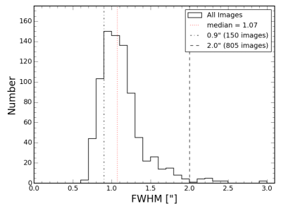
Figure 1: A histogram of the FWHM measured from unsaturated stars for the 838 individual $r$-band exposures taken in the GOODS-N field with the LBC-Red camera. The dot-dashed line represents the largest FWHM ($0\farcs 9$) included in the optimal resolution mosaic. The vertical dashed line represents the cut-off of FWHM$\,=2\farcs 0$ used for the optimal depth mosaic, which includes 805 exposures. The median value of the FWHM distribution, FWHM$\,=1\farcs 07$, is highlighted by the red, dotted line.

2.2 Creating $r$-band Mosaics

For each of the 838 individual exposures, the Gaussian FWHM was measured for unsaturated stars in the FOV, with the median value corresponding to the seeing of the entire exposure. As described in Ashcraft et al. (2018), Otteson et al. (2021) and Redshaw et al. (2022), this allows for a seeing distribution to be created for the entire dataset as shown in Figure 1. The median FWHM for all images is $\sim$1$\farcs 07$, which is marginally larger than the typical seeing conditions on Mt. Graham for $r$-band of $0\farcs 97\pm 0\farcs 06$ (Taylor et al., 2004). Following the prescription from Ashcraft et al. (2018), the optimal depth $r$-band stack was created with all exposures with FWHM$\,\lesssim\!2\farcs 0$, which excludes only the 33 images with the worst seeing ($\sim\!4\%$ of the dataset). The optimal resolution $r$-band stack was created using all images with FWHM $\lesssim$ $0\farcs 9$, which corresponds to the best 150 exposures ($\sim\!18\%$ of the data).

Prior to creating the mosaics, the relative transparency was calculated for each of the 838 exposures following the prescription in Otteson et al. (2021); Redshaw et al. (2022) and McCabe et al. (2022; in prep.). In order to account for the night to night differences in relative atmospheric transparency, the flux ratio between $\sim$100 unsaturated stars was taken with respect to the flux values from the Sloan Digital Sky Survey (SDSS) Data Release 16 (Blanton et al., 2017; Ahumada et al., 2020) in the $r$-band . In this case, a relative transparency value of 1 indicates that the median flux from the $\sim$100 matched SDSS stars in the $r$-band is equal to the flux from the same stars in the individual exposure. Relative transparency values less than 1 indicate that there is less flux received from these stars than expected based upon SDSS $r$-band values. Figure 2 shows the relative transparency for the night of January 17, 2013, where the median transparency varied from $\sim$0.94 to $\sim$0.98. We corrected for these night-by-night transparency differences by simply scaling images by the median transparency offset to achieve a transparency of 1.0 in the affected images.

The optimal resolution and optimal depth mosaics were created by combining individual exposures with swarp (Bertin et al., 2002; Bertin & Amorisco, 2010). Table 1 summarizes some of the key swarp parameters used for creating these mosaics. The choice of parameters is almost identical to those used previously in Ashcraft et al. (2018), except for using a “BACK_SIZE” parameter of 280 pixels for the mesh size, and a “BACK_FILTERSIZE” of 7. The background parameters were increased to compensate for the increased number of bright saturated stars in individual images compared to the U-band data of Ashcraft et al. (2018).

Fig. Set2. Relative transparency of the GOODS-N LBT $r$-band images from January 2013 to March 2014.

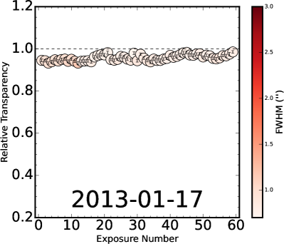
Figure 2: Relative transparency values for the first 59 exposures in the sample from January 17, 2013. The color of each data point represents the median seeing value of $\sim$100 unsaturated stars identified in the FOV. The conditions on this particular night allowed for particularly high transparency. On average, across the entire dataset, the relative transparency is $\sim$80% with some nights between 40-60%. The flux across each image was scaled so that the relative transparency values were equal to unity and uniform from image to image and therefore, night to night. The complete figure set (15 images) for the full dataset is available in the online journal.

Keyword	Value
COMBINE_TYPE	CLIPPED
WEIGHT_TYPE	MAP_WEIGHT
PIXELSCALE_TYPE	Median
CENTER (J2000)	12:36:54.5, +62:15:41.1
IMAGE_SIZE (pix)	6351, 6751
RESAMPLING_TYPE	LANCZOS3
CLIP_SIGMA	5.0
CLIP_AMPFRAC	0.5
BACK_SIZE	280
BACK_FILTERSIZE	7

Table 1: SWARP Configuration Parameters adopted for the $r$-band Mosaics.

2.3 LBC $r$-band Catalogs

SExtractor (Bertin & Arnouts, 1996) was used to identify objects and create photometric catalogs. We developed a SExtractor parameter set which adequately balanced the unique source separation without removing extended, low surface brightness features from their host galaxies. Beginning with the SExtractor parameters used in the Ashcraft et al. (2018) analysis, various parameters were tweaked to optimize object detection and deblending. For the $r$-band catalogs, the deblending parameters “DEBLEND_NTHRESH” and “DEBLEND_MINCONT” were adjusted to more accurately separate objects, especially in the more dense regions of the field. For object detection, a Gaussian filter was used to smooth the image with a convolving kernel (FWHM 2.0 pixels) and a convolution image size of $5\times 5$ pixels. It was found that changing the deblending parameters affected the number of objects detected, but the choice of the smoothing filter did not have a significant impact on number of extracted objects by SExtractor. However, failure to use a smoothing filter resulted in a large amount of spurious detections. The major SExtractor parameters used to create the final $r$-band catalogs are listed in Table 2.

Keyword	Optimized Resolution	Optimized Depth
DETECT_MINAREA	6	6
DETECT_THRESH	1.0	1.0
ANALYSIS_THRESH	1.0	1.0
DEBLEND_NTHRESH	64	64
DEBLEND_MINCONT	0.008	0.004
WEIGHT_TYPE	MAP_RMS	MAP_RMS

Table 2: SExtractor Configuration Parameters adopted for the $r$-sloan Mosaics

A mask image was generated to discard any bright stars and their surrounding corrupted areas during the $r$-band object detection process. The mask was created from the optimal depth image, which had the largest Gaussian wings resulting from the larger FWHM of included exposures. For consistency, the same mask was used for both mosaics. The final object catalogs excluded all objects with the SExtractor FLAGS value larger than 3, and magnitude errors greater than $\sigma$$m_{\rm AB}$ $>$ 0.4 mag. Lastly, photometric zero points were determined by identifying unsaturated stars with AB magnitudes between $r_{AB}$$\simeq\!18$ and $r_{AB}$$\simeq\!22$ mag and matching them to SDSS $r$-band magnitudes. Approximately 170 stars within this magnitude range were verified in the LBC images. Stars with nearby neighboring objects were excluded in order to prevent potentially biased flux measurements. We measured photometric zero points of 28.06 and 28.05 mag for the optimal resolution and optimal depth mosaics, respectively.

3 ANALYSIS

The trade off between the optimal resolution and optimal depth mosaics is clear when looking at the larger and brighter galaxies in the LBT/LBC mosaics. When lower resolution images (FWHM $\gtrsim 1\farcs 0$) are included, the light from galaxies smooths out and substructures are lost within brighter and larger galaxies (see Fig. 3 and Fig. 4). This phenomena is most apparent when comparing bright face-on spiral galaxies ($r_{AB}$$\simeq 17.5-19.5$ mag) from the $r$-band optimal resolution ($0\farcs 9$ FWHM) and optimal depth ($2\farcs 0$ FWHM) mosaics and the U-band optimal depth mosaic ($1\farcs 8$ FWHM; Ashcraft et al. (2018)) to HST-ACS $V_{606}$ images of Giavalisco et al. (2004).

Figure 3 clearly illustrates the power of having both ground based optimal resolution and optimal depth images in addition to high resolution HST imaging. In the top panel, a bar is clearly present in the HST image and the $r$-band optimal resolution mosaic, but is much less discernible in the optimal depth mosaic. This feature is also discernible in the LBT mosaics, especially in the optimal resolution $r$-band mosaic. Of the detectable features in the LBT mosaics, the smallest scale galaxy features are easier to identify in the optimal resolution mosaic. Most notably, we note that in the deeper LBT $r$-band mosaics, extended low-surface brightness flux in the outer parts of the galaxy is present, which is not always apparent in the HST images.

Similar to Figure 3, Figure 4 shows two additional bright galaxies that fall outside of the HST footprint. These galaxies exhibit signatures of star forming clumps within their spiral arms, which are particularly prominent in the optimal depth images. While clumps are observed to be more prevalent at higher redshifts, these optimal depth and resolution mosaics may be useful in determining the origin and ages of the clumps in addition to serving as analogs for high redshift galaxies (Elmegreen et al., 2009a, b; Overzier et al., 2009; Fisher et al., 2014; Adams et al., 2022, and references therein).

The lower-resolution images also make it more difficult to deblend neighboring objects (see Fig. 5). Example Region 2 in Fig. 5 shows a large region, which is detected as one object by SExtractor in the optimal depth, yet lower-resolution mosaic, indicated by a dashed circle, while SExtractor is able to separate the objects within the dashed circle in the higher-resolution mosaic, indicated by solid circles. All magnitudes presented in Fig. 5 are measured in the optimal depth LBT $r$-band, except for the objects within the example 2 dashed circle, which come from the optimal resolution $r$-band catalog. Objects 3, 4, and 6 in Fig. 5 are examples of faint objects detected in the optimal depth LBT image $r_{AB}$ $\gtrsim$ 28.4 mag. Only object 6 was detected in the optimal resolution catalog, which is near its limit for reliable detections, and all three regions show almost no measurable flux above the background levels in the HST F606W filter.

Figure 5 shows a low-surface brightness region in the example of circle 1, which is barely detectable in the HST F606W mosaic. In contrast, the compact object in the example of circle 5 is fainter ($m_{\rm AB}$ $\simeq$ 27.7 mag) than the low-surface brightness region of example 1 ($m_{\rm AB}$ $\simeq$ 26.3 mag), yet its small size and higher-surface brightness makes it easy to detect in the high-resolution HST images.

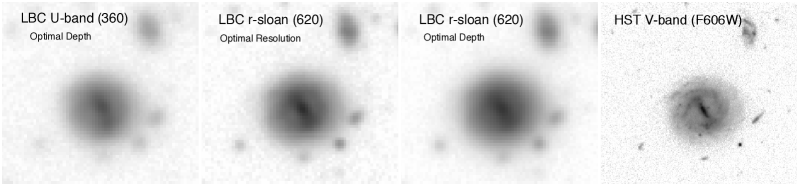
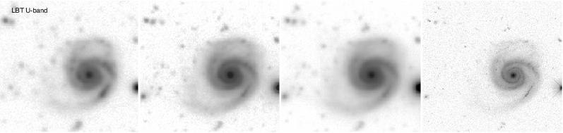
Figure 3: Four bright face-on spiral galaxies in the GOODS-N field, which are also observed in HST CANDELS. The top galaxy has $U_{AB}$ = 20.8 mag and $r_{AB}$= 19.5 mag, the second galaxy has $U_{AB}$ = 18.0 mag and $r_{AB}$= 17.5 mag, the third galaxy has $U_{AB}$ = 19.9 mag and $r_{AB}$= 18.5 mag, and the bottom galaxy has $U_{AB}$ = 19.5 mag and $r_{AB}$= 18.5 mag. The LBC optimal depth U-band image, LBT $r$-band optimal resolution image, LBT $r$-band optimal depth image, and the HST ACS $V$-band (F606W; Giavalisco et al. (2004)) image are shown from the left columns to the right columns, respectively.

Figure 4: Two of the brightest galaxies in the LBC FOV, but outside the HST CANDELS area. The top galaxy has $U_{AB}$ = 18.3 mag and $r_{AB}$ = 16.7 mag, and the bottom galaxy has $U_{AB}$ = 19.2 mag and $r_{AB}$ = 18.3 mag. From left to right, the columns show the optimal depth U-band image, the optimal resolution $r$-band image, and the optimal depth $r$-band image, respectively. Both of these face-on spirals are sufficiently well-resolved spatially that several sub-structure features including clumps and spiral arms. Most of these features can be seen in both the optimal resolution and optimal depth mosaics. However, the features are sharper and easier to distinguish in the optimal resolution mosaic, while some features blur together in the optimal depth mosaic.

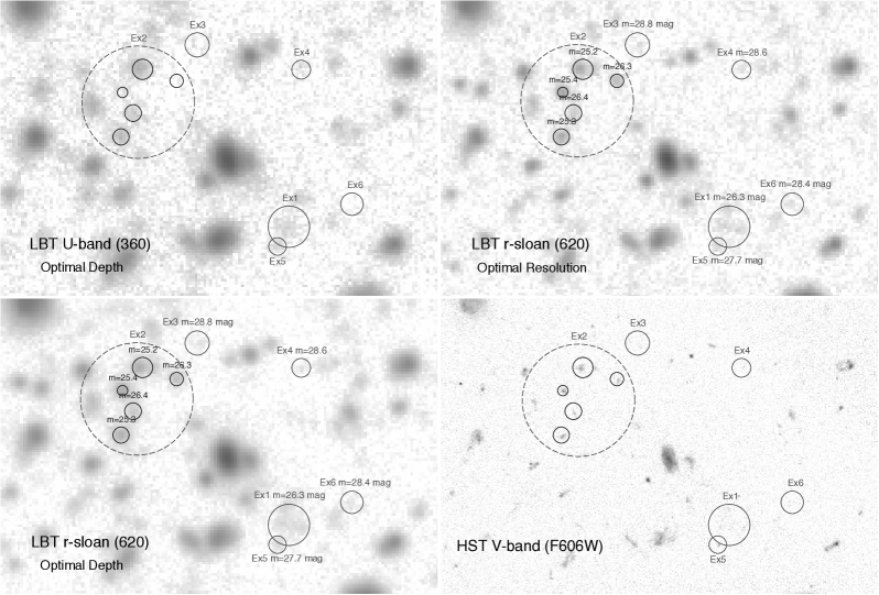
Figure 5: The LBC optimal depth U-band (top left), optimal resolution $r$-band (top right), optimal depth $r$-band (bottom left), and HST ACS $V$-band F606W (bottom right)images are shown for the same region of the GOODS-N field. In this region, the faintest flux detected in the LBT $r$-band mosaics ($r_{AB}$$\simeq$ 28.5 mag for the optimal depth image) is not always discernible in the HST images (see example regions 3, 4 and 6). The smallest objects in the HST V-band (F606W; FWHM$\lesssim$ $0\farcs 68$) are not always detected as single objects in the LBC mosaic catalogs, especially for the lower-resolution optimal depth LBT mosaics. The dashed circle region of example 2 demonstrates an area where SExtractor detected a few separate objects as one in the LBT optimal depth $r$-band mosaic. However, SExtractor was able to deblend objects in the LBT optimal resolution $r$-band mosaic shown by the solid circles within the example region 2 dashed circle. The circle of example 1 shows a low-surface brightness region, which is hard to detect in the HST $V$-band. In contrast, the compact object in the example 5 circle is fainter than the low-surface brightness region of example 1, yet its small size makes it easy to detect in the high-resolution HST images. All magnitudes are measured in the optimal depth LBT $r$-band except for the objects within the example 2 dashed circle, which come from the optimal resolution $r$-band catalog.

3.1 Optimal Resolution versus Optimal Depth LBT $r$-band Mosaics

In order to compare the optimal resolution and optimal depth mosaics, the catalogs described in §2.3 were used to look at object magnitude as a function of FWHM (Figure 6). The solid lines represent the FWHM limits of $\sim$ $0\farcs 65$ and $\sim$ $0\farcs 90$ for the optimal resolution and optimal depth mosaics, respectively. Objects with $m_{\rm AB}$ $\gtrsim$ 29 mag generally have sizes “smaller” than the FWHM limit of the Point Spread Function (PSF), and therefore are not reliable detections. The black dashed and dot-dashed lines represent the effective surface brightness limits for the optimal resolution and optimal depth mosaics, respectively, while the red dashed line denotes the star/galaxy separation.

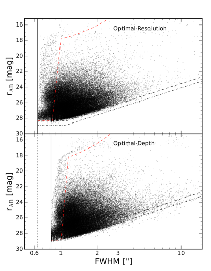
Figure 6: Total SExtractor object magnitude vs. FWHM as measured with SExtractor for the optimal resolution mosaic (top) and the deepest-lower-resolution mosaic (bottom). The solid lines represent the FWHM-limit used in each image, and the black dotted and dotted-dashed lines represent the effective surface-brightness limits for the optimal resolution and optimal depth mosaics, respectively.

For further comparison, the half-light radii measured by SExtractor for both the optimal resolution and optimal depth images for galaxies brighter than $r_{AB}$$\lesssim$ 27 mag is shown in Fig. 7. Unsurprisingly, the half-light radius of the optimal resolution image is consistently smaller than the optimal depth image. The half-light radii distributions peak at $\sim 0\farcs 45$ and $\sim 0\farcs 58$ for the optimal resolution image and the optimal depth image, respectively.

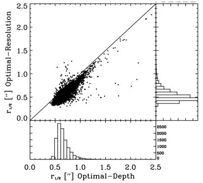
Figure 7: Half-light radius for galaxies with $r_{AB}$$\lesssim$ 27 mag were measured using SExtractor. The optimal resolution image indeed yields consistently smaller half-light radii compared to the optimal depth image.

The SExtractor half-light radii were compared to the equivalent HST V–band catalog of the GOODS-N field from Giavalisco et al. (2004). For this analysis, only galaxies with magnitudes between 18 $\leq$ $m_{\rm AB}$ $\!\leq$ 27 mag as measured in the HST V–band were selected. Figure 8 shows that the radii measured in the optimal resolution image (blue dots) agree slightly better with the HST size measurements with less scatter than the sizes measured in the lower resolution image (red dots). In order to accurately represent intrinsic object sizes, we subtracted the PSF FWHM-values of of $0\farcs 67$ and, $0\farcs 98$ in quadrature from the optimal resolution and depth measurements, respectively ($r_{corr}=\sqrt{r^{2}-(\textrm{FWHM}/2)^{2}}$). For consistency, the PSF-size was subtracted in quadrature for the V–band HST images as well, but since the HST/ACS PSF is so narrow ($0\farcs 08$ FWHM; see Fig. 10a of Windhorst et al. (2011)), this correction had almost no effect except for the very smallest and most faint objects.

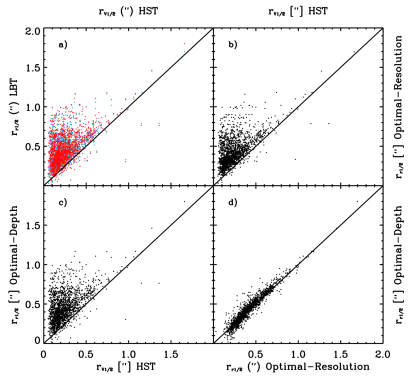
Figure 8: Comparison plots of half-light radius measured with SExtractor for two LBT mosaics, optimal resolution and optimal depth, and the HST V–band. We only included galaxies with 18 mag $\leq$ $r_{AB}$ $\leq 27$ mag. All half-light radii plotted have been corrected using $r_{corr}=\sqrt{r^{2}-(\textrm{FWHM}/2)^{2}}$. Half-light radius for the optimal resolution (blue) and lower-resolution optimal depth (red) images are compared to the half-light radius for the HST V–band (a; Giavalisco et al. (2004)). The optimal resolution (b) or the optimal depth (c) half-light radius are compared to the HST V–band. The bottom right panel (d) compares the optimal depth to the optimal resolution half-light radius measurements.

4 Analysis

4.1 Tidal Tails and Merging Galaxies

We visually inspected the LBT GOODS-N $r$-band mosaics for signs of galaxy interactions such as tidal tails, diffuse plumes, and bridges. Approximately, 60 galaxies were found that were candidates for interactions, the 30 most obvious galaxies were selected for the sample of interacting galaxies. These galaxies are listed in Table 3 along with their classification, redshift, and position. Interacting systems can resemble multiple types, especially when looking at both the HST and LBT images of the same systems. Each of these classifications is defined as follows, following Elmegreen et al. (2007):

• Diffuse: Interactions are defined by diffuse plumes with small, star forming regions.

• Antennae: Antennae type interactions resemble the local Antennae system with long tidal tails and signs of possible double nuclei.

• M51: M51 interactions consist of a main spiral galaxy with a tidal arm that forms a bridge towards a companion.

• Assembly: Assembly types are irregular galaxies that appear to be merging and are made up of small pieces.

• Equal mass: Equal mass types appear as though two similar sized galaxies are in the process of merging.

• “Shrimp”: ‘Shrimp” types are characterized by a single prominent arm and uniformly distributed star forming clumps without signs of a central nucleus or core.

• Tidal tail: Tidal tail interactions exist when both interacting galaxies still resemble their pre-merger shape, but have an extended tidal tail which indicates a recent interaction.

Since this sample of interacting galaxies was selected with the goal of observing extended flux in the outer regions of the galaxies, it is inherently not a complete sample of interacting galaxies in the GOODS-N field. After the galaxies were selected, HST imaging was examined if available. For a complete sample, deeper HST imaging and spectroscopic redshifts would be required to confidently confirm galaxy morphology and interacting systems. However, since the $r$-band mosaics are $\gtrsim$90% complete to SB levels of $m_{\rm AB}$ $\lesssim$ 31 mag arcsec^-2, these 30 galaxies constitute a representative sample to this SB limit. While HST imaging is not available for each galaxy in our sample, Appendix A shows the $r$-band and U-band optimal depth images and HST (F275W, F336W, F435W, F606W, F775W, F814W, F850LP, F105W, F125W, F160W, which correspond to the NUV, u, b, v, i, I, z, Y, J, H filters) images when available. Our sample covers objects with tidal features and redshifts in the range of $z\,\simeq$ 0.03–1.0.

Below we briefly comment on a small subset of the 30 interacting galaxies from Table 3. Full discussion and LBT/HST imaging of these galaxies can be found in Appendix A.

• Galaxy 1: This galaxy appears to have both a plume and a tidal tail in the LBT $r$-band (Figure 11). The plume appears above the galaxy, while the tidal tail extends towards the lower left. These features are not easily identifiable in HST imaging, but become apparent after smoothing the F160W data. When looking at high resolution imaging with HST F336W and F275W, this galaxy appears to be composed of multiple clumps.

• Galaxy 3: This galaxy has a diffuse tail above the galaxy that is present in both the LBT and HST imaging (Figure 12). However, the LBT $r$-band image also shows a second tidal tail below the galaxy that is not present in the HST imaging.

• Galaxy 6: LBT $r$-band imaging of this galaxy shows diffuse, tidal debris to the right side of the galaxy, which is not easily identifiable in the HST imaging (Figure 13). The tidal debris appears to make a loop around the galaxy in the deep $r$-band image.

These examples show that deep $r$-band imaging with the LBT/LBC is critical for finding low surface brightness regions such as tidal tails, plumes, and streams that are not otherwise identifiable with HST imaging. These data, along with multiwavelength HST imaging and the U-band data from Ashcraft et al. (2018) should be used in future studies to study the ages, colors, and properties of these galaxy interactions.

Table 3: List of Interacting and Merging Galaxies in the GOODS-N

Number	Interaction Type	z	RA	DEC	Number	Interaction Type	z	RA	DEC
1	Antennae	0.4571	189.143651	62.203670	16	Diffuse	0.487	189.546198	62.073688
2	Tidal Tail	0.3752	188.991511	62.260236	17	Equal	0.0341	189.046012	62.275677
3	Diffuse	0.5303	189.308326	62.343553	18	Diffuse	0.5608	189.531696	62.088388
4	Shrimp/Equal	0.2991	189.399092	62.302951	19	Tidal Tail	–	188.878151	62.105181
5	M51	0.2531	189.220288	62.302170	20	Diffuse	–	188.849864	62.105759
6	Tidal Tail	0.3061	189.469709	62.274555	21	Diffuse/Tidal Tail	–	189.316382	62.440579
7	Equal	0.6374	189.027615	62.164315	22	Equal/Diffuse	–	189.279264	62.454440
8	Diffuse	0.4401	189.446132	62.275576	23	Tidal Tail	–	189.270045	62.458354
9	Tidal Tail/M51	0.3771	189.420590	62.254833	24	Tidal Tail	–	189.495589	62.399123
10	Shrimp	–	189.080363	62.301563	25	Assembly	–	189.183626	62.357549
11	Tidal Tail/Diffuse	0.7985	189.191198	62.107990	26	Diffuse	–	189.208981	62.458493
12	Diffuse	–	189.222929	62.103161	27	Tidal Tail	0.3348	189.216085	62.427977
13	Assembly	0.93744	189.195308	62.116697	28	Antennae	–	189.153633	62.414972
14	Antennae	0.2776	189.622461	62.280396	29	Diffuse	–	189.086340	62.419340
15	Equal/Tidal Tail	0.456	189.547345	62.175356	30	M51	–	189.145952	62.453802

4.2 Implications for the Extragalactic Background Light

The powerful ability of the optimal depth mosaics to highlight extended, low surface brightness (SB) features in the outskirts of galaxies can be utilized to investigate the contribution of diffuse galaxy light to the EBL. For galaxies brighter than $m_{\rm AB}$ $\simeq$21.5 mag, the azimuthally averaged radial surface brightness (SB) profiles were measured using the custom IDL program galprof for both the optimal resolution and optimal depth $r$-band mosaics. This left a sample of 360 galaxies suitable for the surface brightness analysis after eliminating galaxies in close proximity to bright stars or the edge of the FOV. The 360 galaxy profiles were analyzed and the excess light in the optimal depth profile was ranked as “confident”, “potential”, or “identical”. Surface brightness profiles ranked as “confident” exhibited a $\sim$1.0 mag arcsec^-2 difference in the two profiles over multiple radial points or had multiple data points between the two profiles that were separated by more than the 1$\sigma$ uncertainty ranges plotted. Profiles ranked as “potential” were classified by a $\sim$0.5 mag arcsec^-2 difference between the two profiles. However, typically the uncertainty ranges in the optimal depth and resolution data points encompassed the corresponding data point, which did not allow for as confident of a classification. The majority of the surface brightness profiles were identified as “identical”, where there was no apparent difference between the optimal depth and optimal resolution profiles.

Prior to analyzing the surface brightness profiles, we measured the surface brightness sky limits at which the two mosaics began to significantly differ. In order to accomplish this, model galaxies with pure exponential disk profiles matching the size of actual galaxies with $m_{\rm AB}$ $\simeq$19–21.5 mag were created. Approximately 250 non-saturated stars were used to create a model PSF-star for both the optimal resolution and optimal depth mosaics. The model galaxies were then convolved with the corresponding PSF and random background pixels were sampled to create a background map. Then, galprof was run to create surface brightness profiles of the model galaxies. In this analysis, we find the optimal resolution and depth profiles deviated at surface brightness levels of $\mu^{AB}_{r}$ $\sim$31 mag arcsec^-2.

Figure 9 shows a representative selection of 20 out of 360 surface brightness profiles for galaxies in the optimal resolution (blue) and optimal depth (red) mosaics. 16/20 do not exhibit any distinguishable difference between the two profiles to $\mu^{AB}_{r}$ $\lesssim$31 mag arcsec^-2 between the profiles and were categorized as “identical”. Galaxies A, B, C, and D are four examples of galaxies that were ranked as “confident” or “potential” candidates for having significant additional light in the optimal depth surface brightness profiles. Galaxies A and D were categorized as “potential” since they exhibited $\sim$0.5 mag arcsec^-2 differences in surface brightness with both profiles being within the uncertainty ranges of the other. However, galaxies B and C show larger, more robust differences between the optimal depth and resolution profiles.

Driver et al. (2016, Fig. 2) showed that the number density of galaxies in the $r$-band peaks at $m_{\rm AB}$ $\simeq$ 19–24 mag. Thus, this subset of galaxies constitutes a representative sample of galaxies which significantly contributes to the EBL to surface brightness levels of $\mu^{AB}_{r}$ $\lesssim$ 31 mag arcsec^-2, where the background levels of the optimal depth and optimal resolution mosaics begin to differ. Of the 360 galaxies with surface brightness profiles, only 19 were labeled as “confident” and 32 galaxies were labeled as “potential”. Therefore, 5-14% of galaxies in this sample have excess flux in their outskirts out to surface brightness levels of $\mu^{AB}_{r}$ $\lesssim$ 31 mag arcsec^-2, which could contribute to missing, diffuse EBL light as summarized by Driver & Robotham (2010); Driver et al. (2016) and Windhorst et al. (2018). However, the possibility of more uniform, missing flux from all galaxies cannot be ruled out as it would be diffuse enough across the LBT FOV where it would be removed during the swarp background subtraction process. This excess $r$-band light could be the result of an older population of stars in the galaxy outskirts, star formation being traced by H$\alpha$ out to redshifts of $z\lesssim$ 0.2, or tidal tails from galaxy interactions.

This fraction of galaxies with excess light in the optimal depth images is also represented in Figure 10. These galaxies are most apparent in the bottom panel where the magnitude difference between the optimal resolution and optimal depth images for galaxies brighter than 21.5 mag. This panel shows a population of $\sim$19 galaxies with optimal resolution – optimal depth magnitudes greater than 1.0 mag, which corresponds to the number of surface brightness profiles ranked as “confident”. There are $\sim$30 galaxies that exist with a magnitude difference greater than 0.5 mag, which would match up with $\sim$50% of the “potential” profiles as having significant excess light in in the optimal depth surface brightness profiles.

In addition to the surface brightness profile analysis, the total contribution of light in galaxy outskirts to the EBL was calculated by integrating the normalized galaxy counts up to the optimal resolution and optimal depth completion limits of $\sim$27 mag following the methods in Driver et al. (2016); Carleton et al. (2022) and Windhorst et al. (2022). The contribution to the EBL from the outskirts of galaxies is represented by the difference between the total energy from the optimal depth and optimal resolution integrated counts. This analysis showed that the total EBL contribution is 0.19 $\rm{nW\,m^{-2}\,sr^{-1}}$ (3.52 - 3.33 $\rm{nW\,m^{-2}\,sr^{-1}}$), which is $\sim 5$% of the total EBL in the Sloan $r$-band. Since these three independent methods of searching for additional light in the outskirts of galaxies provide similar results, it can confidently be stated that only a small fraction ($\sim$ 5-14%) of extra light in galaxy outskirts is available to contribute towards missing EBL light.

Fig. Set9. Surface brightness profiles with $r_{AB}$$\simeq$21.5 mag

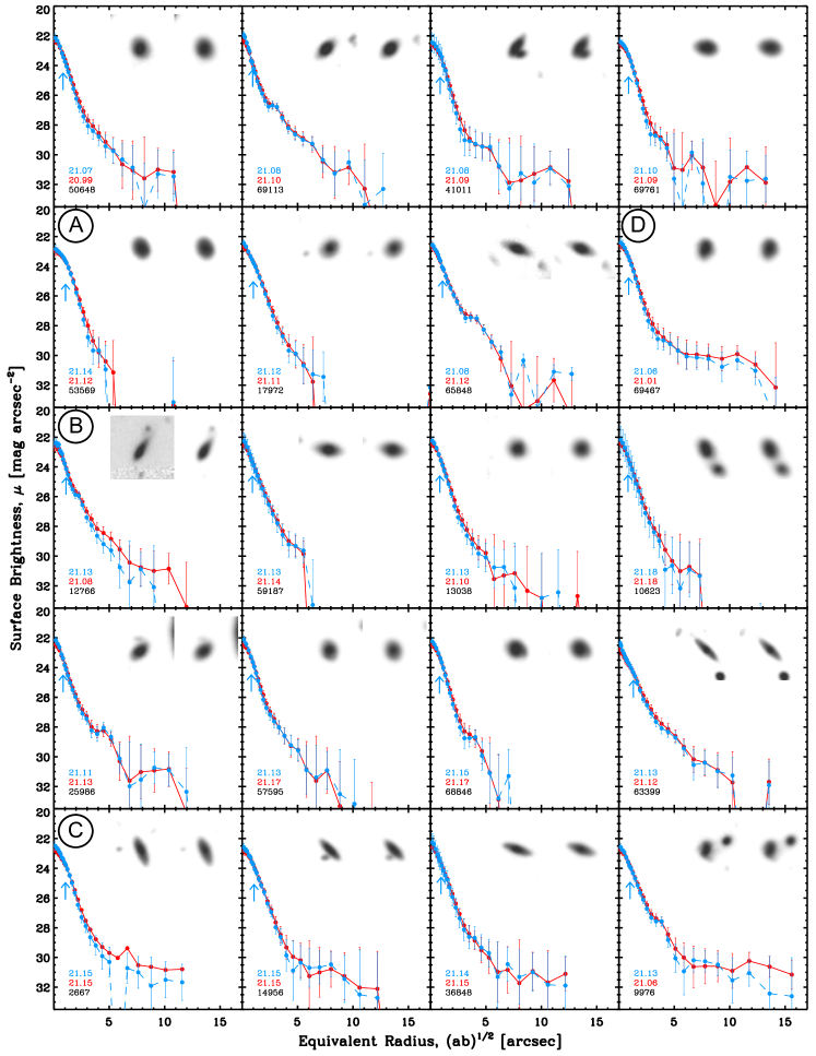
Figure 9: Radial surface brightness profiles for 20 of the 360 brightest objects with $r_{AB}$$\lesssim$21.5 mag. The blue data points show the surface brightness profile for the optimal resolution image, while the red points show the corresponding profile for the optimal depth image. The total integrated $r_{AB}$magnitudes from the profiles are listed in the lower left corner. The blue arrow represents the half-light radius measured with SExtractor. The galaxy inset images show the optimal resolution (left) and optimal depth (right) images. Galaxies A, B, C, and D clearly show excess flux in the outskirts of the optimal depth surface brightness profiles at levels brighter than $r_{AB}$$\lesssim$31 mag. The complete figure set showing all 360 surface brightness profiles is available in the online journal.

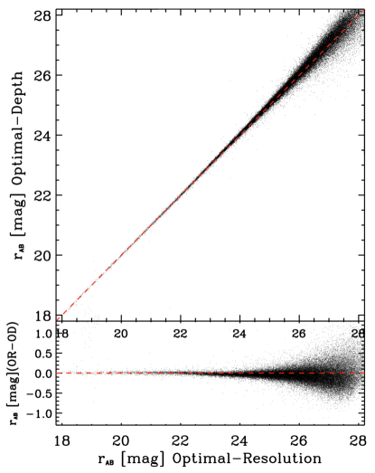
Figure 10: Comparison of total $r$-band magnitudes measured by SExtractor, using dual image mode, in the optimal resolution (OR) and the optimal depth (OD) mosaics. The bottom panel shows the OR - OD magnitude difference objects in the two catalogs. On average, there is little excess light in the optimal depth images than observed in the corresponding optimal resolution image. This aligns with what is observed in the surface brightness profile analysis where $\lesssim$10–14% of galaxies are observed to have excess $r$-band flux in their outskirts.

5 SUMMARY AND CONCLUSIONS

838 $r$-band exposures ($\sim$ 28 hours) were obtained between December 2012 and January 2014 of GOODS-N in order to examine the trade-off between optimal image resolution and depth. Following the seeing sorted stacking method detailed in Ashcraft et al. (2018), the best seeing images were stacked to create optimal depth and optimal resolution mosaics. The optimal depth mosaic was found to be necessary for the study of low surface brightness regions presented in this work. The sacrifice in resolution was complemented by increased surface brightness sensitivity down to $\mu^{AB}_{r}$ $\leq 31$ mag arcsec^-2.

The main challenge for photometric measurements was to overcome the natural confusion limit for separating objects, which occurs once faint objects are closer than $\sim 1\farcs 0$ in ground based images (Windhorst et al., 2011). In order to accurately deblend sources in the mosaics, SExtractor in dual image mode was utilized in order to deblend and detect objects using the optimal resolution mosaic. Within the optimal depth and optimal resolution mosaics, objects can be detected to $m_{\rm AB}$ $\sim$29 and $m_{\rm AB}$ $\sim$28.5 magnitudes, respectively.

A collection of 30 candidate interacting galaxies were investigated along with their low-surface brightness features. For the majority of these systems, the galaxies were not resolved sufficiently for detailed morphological classification. For the sample galaxies that did fall within the HST footprint, the higher resolution images were used for interaction classification following the methods of Elmegreen et al. (2007) and the diffuse flux/tidal tails were described. Future studies can utilize the LBT U-band and $r$-band mosaics along with additional filters to continue to study the properties of these 30 interacting galaxies. Specifically, the colors of the diffuse plumes and tidal tails can be measured to gain more insight into the age and properties of these stellar populations.

Lastly, surface brightness profiles were measured for the 360 brightest galaxies with $r_{AB}$$\lesssim$ 21.5 mag in both the optimal resolution and optimal depth mosaics. Galaxies with magnitudes $m_{\rm AB}$ $\lesssim$ 21.5 provide a representative sample of galaxies that could contribute significantly to the Extragalactic Background Light in the $r$-band (Driver et al., 2016). These surface brightness profiles show marginal differences between the optimal resolution and optimal depth mosaics to surface brightnesses of $\mu^{AB}_{r}$ $\sim$31 mag arcsec^-2. Only 19/360 galaxies confidently exhibited excess flux in the optimal depth radial profiles, while another 32/360 galaxies were categorized as “potentially” having excess flux in the outskirts.

As a result, on average, we conclude that only $\sim$5-14% of extra light in the outskirts of galaxies are likely to contribute to the Extragalactic Background Light out to surface brightness levels of $\sim$31 mag arcsec^-2. The EBL contribution from the outskirts of galaxies was found to be $\sim$5% of the EBL determined from the integrated galaxy counts. We find that while there is some contribution to the EBL from diffuse light in galaxy outskirts, there is not enough of a contribution in the $r$-band to close the discrepancy between direct EBL measurements (Puget et al., 1996; Hauser et al., 1998; Matsumoto et al., 2005, 2018; Lauer et al., 2021; Korngut et al., 2022) and predicted values (Driver et al., 2011, 2016; Andrews et al., 2018).

Appendix A Tidal Tails and Mergers

Below, we briefly describe the full sample of different tidal tail and merging galaxy candidates. Galaxies which reside within the HST FOV are shown first.

1. 

    

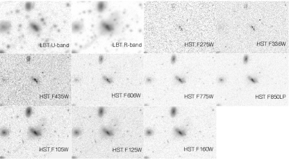
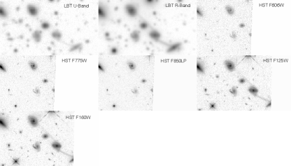
   Figure 11: Galaxy 1 (top): A galaxy with long extended tidal tail and diffuse flux seen in LBT $r$-band and has a $z_{spec}$ = 0.457. The galaxy is visible in HST images from F275W-F160W, with only a double lobe being visible in the UV. The diffuse flux and tidal tail is visible in the NIR wavelengths, especially bright in the F105W. Galaxy 2 (bottom): Multiple spiral galaxies interacting with two long tidal tails visible linking the galaxies. The galaxies all have either spectroscopic or photometric $z\sim$ 0.375. This system is only partially visible in HST imaging with best views being in the J and H-bands. Only one of the tidal streams is clearly visible in the U-band.

2. In the $r$-band, there is a diffuse plume above the galaxy and a long tidal tail downward to the left in the image (top galaxy in Fig. 11). This galaxy is inside the HST FOV, but the tidal debris is not clearly visible without smoothing the data, and is most prominent in the F160W. It has a clear dust lane through the center perpendicular to the tidal tails visible in the HST optical wavelengths. In the F160W image, the dust lane disappears, so that two distinct cores become visible. Multiple brighter clumps of this galaxy are seen in the HST F336W and F275W images. Since it is detected in both x-ray (Wang et al., 2016) and radio (Biggs & Ivison, 2006), it may have outflows or cooling flows associated with an AGN. Other studies have classified this galaxy as a starburst, high-excitation narrow-line radio galaxy, and merging, and measured a redshift of $z_{spec}$ = 0.457 (Wirth et al., 2004).

3. Galaxy 2 shows a clear recent interaction with at least two galaxies, possibly a third, with measured redshifts, z$\simeq$ 0.375 (bottom images in Fig. 11). There is a tidal tail between the two galaxies in the bottom right, which is also visible in the LBT U-band. Another tidal tail in the opposite direction probably links the central galaxy to a third spiral galaxy in the upper left. This tidal tail barely is detectable in the U-band mosaic, which could be due to multiple reasons including an older stellar population in the interaction. Unfortunately, this system of galaxies is on the edge of the HST FOV and only the less dominant tidal tail is visible in the HST WFC3 IR images.

4. An elliptical galaxy with a diffuse debris tail visible in the $r$-band and partly in the U-band mosaic (top galaxy in Fig. 12). It has a $z_{spec}$ = 0.530 (Moran et al., 2007). The diffuse flux above the main galaxy has a similar photometric redshift to the main galaxy, and can been seen in the HST V to H-bands. There appears to be a tail of debris coming from the bottom of the main elliptical galaxy, and the brightest clump in the stream has a $z_{spec}$ = 0.533 (Moran et al., 2007).

   

    

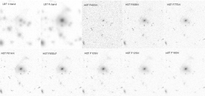
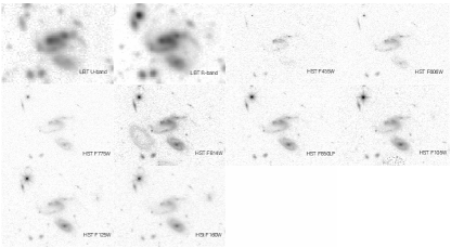
   Figure 12: Galaxy 3 (top): Elliptical galaxy with diffuse flux seen prominently above the galaxy in $r$-band and only slightly in U-band, and has a $z_{spec}$ = 0.530. A smaller galaxy, out of the FOV in the figure, has the same spectroscopic redshift, and could be associated with the tidal interaction. In addition, there is a long tidal stream with clumps below the main galaxy. Galaxy 4 (bottom): Obvious merging system with multiple tidal arms and a $z_{spec}$ = 0.299. From the the HST images, there appears to be no distinct core for the merging galaxy.

5. Reminiscent of the nearby system, Stephan’s Quintet, there are at least three similar size spiral galaxies involved with this interaction (bottom set of images in Fig. 12). Two of the galaxies are already merging, while a third appears to be gravitationally influencing one of the tidal tails. In the HST imaging, the tidal arms are visible in all bands, and the system has $z_{spec}$= 0.299 (Wirth et al., 2004).

6. Similar to M51, galaxy 5 (top galaxy in Fig. 13) has a diffuse tidal stream on the bottom right linking it to a smaller companion galaxy and with a $z_{spec}$ = 0.253 (Wirth et al., 2004). The HST images show a dust lane through the center of the galaxy and parallel to the diffuse stream. In the centers of both the main and the companion galaxies, no detectable flux is present in both the F336W and F275W filters.

   

    

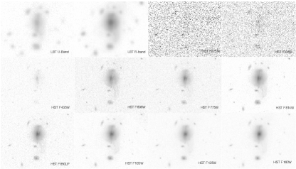
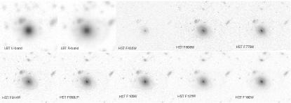
   Figure 13: Galaxy 5 (top): There is diffuse debris on the bottom right side toward a smaller companion galaxy, similar to a M51 type system. This is one of only two galaxies in our sample with both F275W and F336W imaging. It has $z_{spec}$ = 0.253 (Wirth et al., 2004). Galaxy 6 (bottom): There is smooth diffuse tidal debris to the right of the galaxy that appears to make a loop from back to front, but is only seen in the LBT $r$-band and not the U-band. The HST imaging shows a very bright core surrounded by a disk. It has $z_{spec}$ = 0.306 (Wirth et al., 2004).

7. There is smooth diffuse tidal debris visible in the LBT $r$-band to the right of the galaxy that appears to make a loop around the galaxy, but is not detectable in the LBT U-band (bottom galaxy in Fig. 13). From the HST imaging, it appears as a face on disk galaxy with a very bright center and possible bar. The tidal debris is only marginally seen without smoothing. It has been classified as a broad-line AGN and a measured $z_{spec}$ = 0.306 (Wirth et al., 2004).

8. An edge-on disk galaxy, which has been identified as an AGN (top galaxy in Fig. 14). It has extra diffuse flux upward and to the left, which is seen in both $r$-band and $U$-band. In addition, it has a possible approximately equal size grazing companion. The main galaxy has $z_{spec}$ = 0.637 (Barger et al., 2008), but the potential companion galaxy to the right is not spectroscopically confirmed to be at the same redshift. However, the small galaxies to the left have $z_{spec}$ = 0.632 (Barger et al., 2008).

   

    

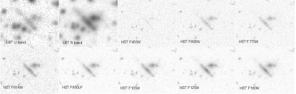
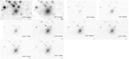
   Figure 14: Galaxy 7 (top): Galaxy 7 is an edge-on disk galaxy with an AGN. It has extra diffuse flux upward and to the left, which is seen in both LBT $r$-band and $U$-band, and a possible equal size grazing companion. Across most of the HST images, the diffuse flux is visible. The main galaxy has $z_{spec}$ = 0.637 (Barger et al., 2008). Galaxy 8 (bottom): There is smooth, diffuse debris on the left side of the galaxy only seen in the LBT $r$-band mosaic and is only marginally detectable in some of the redder HST images. The HST images show a bright core with a possible disk, but no spiral structure. It has $z_{spec}$ = 0.440 (Wirth et al., 2004).

9. There is smooth, diffuse debris to the left of the central galaxy seen in the LBT $r$-band , while the U-band only shows background objects (bottom galaxy in Fig. 14). The galaxy has $z_{spec}$ = 0.440 (Wirth et al., 2004). It has also been categorized as a S0/spheroid galaxy, which is confirmed by the HST images, as well as a high-excitation narrow-line radio galaxy (Wirth et al., 2004). The redder HST filters also show the diffuse flux in the same location as the LBT $r$-band.

10. Appearing as an elliptical galaxy, but it clearly has rings with recent star forming clumps visible in the HST images (top galaxy in Fig. 15). The small bright object to its lower left has the same redshift $z_{spec}$ = 0.377 (Wirth et al., 2004). It appears to be a smaller galaxy being tidally disrupted and absorbed by the larger galaxy. In the LBT $r$-band, there appears to be even more diffuse tidal arms that are not easily visible in the HST imaging. Auxiliary data includes a detection in the radio by the VLA (Morrison et al., 2010). The bright galaxy to the upper left is a foreground interloper.

    

     

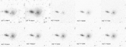
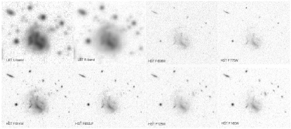
    Figure 15: Galaxy 9 (top): A bright face-on spiral galaxy with a small companion galaxy in the lower left of the image, which is being absorbed by the main galaxy. The core of the companion galaxy is seen in all the HST images, while the brighter galaxy to the upper left is a foreground interloper. Both the main spiral and companion galaxy have confirmed spectroscopic redshifts of $z_{spec}$ = 0.377 (Wirth et al., 2004). Galaxy 10 (bottom): A clearly merging system, with signs of remnants of at least two distinct galaxies. There is one dominant arm curving from the top of the galaxy downward to the right. Several clumps of possible recent star formation are visible within the tidal arm.

11. At least two merging galaxies with the central regions of each galaxy still visible, but distorted (bottom galaxy in Fig. 15). From the LBT observations, there appears to be a tail coming from top and curving around to the right. From the Elmegreen et al. (2007) designations, this galaxy could be categorized as a shrimp type based on its shape and features visible in the different imaging. There is no available redshift for this galaxy.

12. This system appears to have 3 elliptical galaxies with a long diffuse stream toward the upper left corner linking to a possible 4th galaxy in the system (top system of galaxies in Fig. 16). With redshifts of $z\,=$ 0.798 (Treu et al., 2005), these red galaxies are almost not detectable in the LBT U-band. The redder HST filters show the same diffuse stream visible in the LBT $r$-band at low surface brightness levels.

    

     

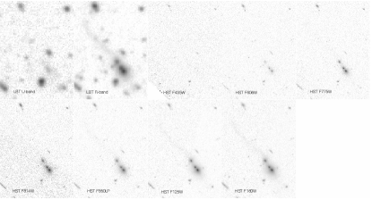
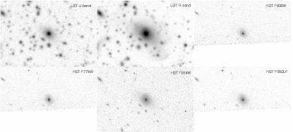
    Figure 16: Galaxy 11 (top): Three distinct elliptical galaxies are visible in the HST imaging, along with a diffuse stream linking to a possible 4th galaxy. The tidal stream is only detectable in the LBT $r$-band , as well as the redder HST filters. For the bluest filters with data (LBT U-band and HST $b$-band), there is only a very limited amount of flux detected even for the main galaxies. This system has a redshift of $z\,=$ 0.798 (Treu et al., 2005). Galaxy 12 (bottom): Another elliptical galaxy; however, there is only one galaxy with a diffuse plume surrounding it and no evidence of a tidal stream of flux. The most prominent area of diffuse flux is outside the HST FOV, except for the I-band (F814W). (The HST F814W image also shows a filter ghost).

13. An elliptical galaxy surrounded by diffuse plumes with the most prominent plume to the lower left (bottom galaxy in Fig. 16). It is on the edge of HST FOV, and does not have any redshift information. Only the HST I-band (F814) image shows the entire region around the galaxy and there does appear to be diffuse flux around the galaxy in this filter. However, it would be easy to miss without re-binning or smoothing the HST data.

14. This is a good example of where HST imaging was critical to confirm that it is an interacting system (Fig. 17). Also, it is the highest redshift galaxy in our sample with $z_{spec}$= 0.937 (Barger et al., 2008). The HST image shows a second possible distinct core at the top of the galaxy, or a starburst clump. The core near the center is not visible in the bluer filters, which indicates a dusty galaxy. There are multiple clumpy objects around the main galaxy, which could be associated with the main merging system.
    

    The following objects are completely outside the HST FOV. In Figs. 18 – 25 only the optimal depth LBT images in the U-band on the left and the $r$-band on the right are shown. Some of the objects are in the footprint for other surveys including Herschel, Spitzer, VLA, and Chandra.

    

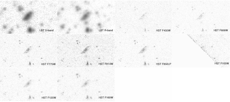
    Figure 17: Galaxy 13: An irregular galaxy with signatures of being in a merger, including a possible second core, or a recent star-forming clump. It is the highest redshift galaxy in our sample and has $z_{spec}=$ 0.937 (Barger et al., 2008), which is why HST imaging was key in confirming that it has morphology of a recent interaction.

15. A galaxy with long tidal streams reminiscent of the Antennae galaxy, but the central region is unresolved (top galaxy in Fig. 18). The diffuse tidal streams are not seen seen in the U-band, except for a few faint spots along the tails. At a redshift of $z_{spec}$ =  0.277 (Casey et al., 2012), the U-band corresponds to NUV flux, which means there is little evidence of recent star formation in these tidal streams. The galaxy was detected by both Herschel (infrared; Casey et al. (2012)) and VLA (radio; Biggs & Ivison (2006)).

    

       

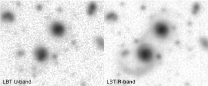
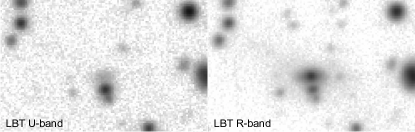
    Figure 18: Galaxy 14 (top): A merging system with a long extended tidal tail to the right and a smaller tail with diffuse flux to the left. It is only significantly detected in the LBT $r$-band and has $z_{spec}$ = 0.277 (Casey et al., 2012). Galaxy 15 (middle): Two galaxies of equal size with multiple extended streams, including a bridge between the galaxies, and a redshift of $z_{spec}$ = 0.456 (Casey et al., 2012) is measured for the top galaxy. The diffuse light in the streams is not easily visible in the U-band, but there appears to be potential star forming clumps. Galaxy 16 (bottom): A red galaxy with diffuse debris to the upper left only detected in $r$-band and a possible redshift of $z_{phot}$ = 0.48 (Rafferty et al., 2011).

16. Two galaxies with extended flux in tidal tails seen in the LBT $r$-band , but only the brightest clumps are in the tails are detectable in the U-band (middle system of galaxies in Fig. 18). The system was detected in the infrared by Herschel and Spitzer, and the top galaxy is associated with a radio source (VLA; Morrison et al. (2010)). The bottom large galaxy is interacting with the smaller galaxy to the left, while the top galaxy has $z_{spec}$= 0.456 (Casey et al., 2012).

17. A very red galaxy, probably elliptical/S0 type galaxy, which is only barley visible in the LBT $U$-band. This galaxy is surrounded by diffuse plumes and has a stream to the upper left (bottom galaxy in Fig. 18). From the literature, it has a photometric redshift of $z_{phot}$= 0.48 (Rafferty et al., 2011).

18. Two large irregular galaxies just outside the HST FOV (top galaxy system in Fig. 19). There are multiple star forming clumps around the two galaxies, which are most likely physically associated based on their colors. The larger galaxy on the right side appears to have a M51 like bridge with the small galaxy to it’s right. They are at a low redshift of $z_{spec}$ = 0.0366 (Wirth et al., 2004).

    

       

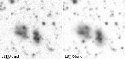
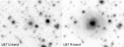
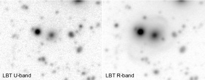
    Figure 19: Galaxy 17 (top): Two large distorted galaxies with antenna like main regions and $z_{spec}$ = 0.0336 (Wirth et al., 2004). Both look similar in the $r$-band and U-band, and the galaxy on the right is also interacting with a smaller galaxy to the lower right. Galaxy 18 (middle): A large diffuse shell of flux is seen only in the $r$-band and as a $z_{spec}$ = 0.560 (Albareti et al., 2017). Galaxy 19 (bottom): A galaxy with long extended diffuse plumes and loops around the galaxy, distinctly visible in $r$-band, with one stream of flux partially detectable in U-band.

19. In the $r$-band there is a large extended shell of diffuse light around the galaxy (middle galaxy in Fig. 19), which is not seen in the $U$-band. This galaxy has $z_{spec}$ = 0.560 (Albareti et al., 2017). The diffuse shell could be a signature of a recent merger.

20. A galaxy with long extended diffuse plumes and loops around the galaxy that is only seen in the LBT $r$-band (bottom galaxy in Fig. 19). There is one tidal stream in the bottom left, which has detectable flux in the corresponding U-band area.

21. Another galaxy with rings of diffuse light surrounding it (top galaxy in Fig. 20). The outer most ring is only seen in the LBT $r$-band, and could be a sign of a recent merger. There is no indication of interaction with any other galaxies nearby it, and no available redshift information.

    

     

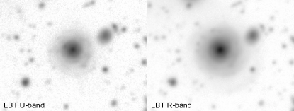
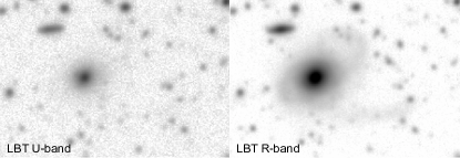
    Figure 20: Galaxy 20 (top): A galaxy with rings of diffuse light around it, with the outer most ring only noticeable in the LBT $r$-band. Galaxy 21 (bottom): An elliptical galaxy with one stream interacting with a much smaller nearby galaxy, and a large diffuse plume above the galaxy. Only potential star-forming clumps along the tidal stream are visible in the U-band.

22. An elliptical galaxy with one stream interacting with a much smaller nearby galaxy, and a large diffuse plume above the galaxy (middle galaxy in Fig. 20). This extended diffuse light is not detected in the U-band, except for discreet clumps along the tidal arm, which are most likely associated with recent star-formation.

    

    Figure 21: Galaxy 22: In the $r$-band, there is a diffuse plume surrounding the central galaxy, along with a couple of bubble like features at the bottom of the galaxy toward another similar size galaxy. Only the main bubble feature is detected in the U-band.

23. Diffuse plumes surround the galaxy in the center of the image, as well as a couple of bubbles, or loop features at the bottom (bottom galaxy in Fig. 22). In the U-band, the majority of the diffuse flux is not detected with only the brighter bubble feature visible. For galaxies within this field, there is no redshift information. The main galaxy could be interacting with multiple galaxies around it, including the similar size elliptical below it, and a galaxy farther to the right following one of the tidal streams.

24. An interesting system with potentially multiple galaxies interacting (top system of galaxies in Fig. 22). There is a larger elliptical at the of bottom of the image with a bridge to a galaxy above it, and a tidal stream extending even farther above it. Without redshift information, it is unknown if the various objects along the tidal tail are gravitationally associated with the interaction.

    

     

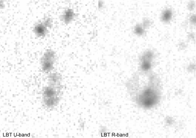
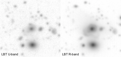
    Figure 22: Galaxy 23 (top): A long diffuse stream is running from the bright galaxy at the bottom to the top of the image, which is not as clearly defined in the U-band. There is a bridge visible in both the $r$-band and the U-band linking the main galaxy to a slightly smaller one. Galaxy 24 (bottom): A galaxy with extended flux along the top and right portion seen in LBT $r$-band and partly visible in the U-band. It appears to be a face-on disk with multiple star-forming clumps and possibly interacting with galaxy above it.

25. A face-on disk galaxy with multiple star-forming clumps and an extended flux feature on the top and left side of galaxy (bottom galaxy in Fig. 22). While most noticeable in the $r$-band, there are a few brighter spots visible in U-band. Another galaxy without any redshift information.

26. An assembly type with two diffuse bridges linking two brighter clump cores (top galaxy in Fig. 23). The left bridge connecting the cores is much fainter in the U-band compared to the rest of the components of the system. There is no redshift information available for this system.

    

     

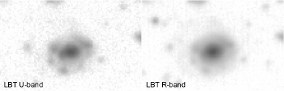
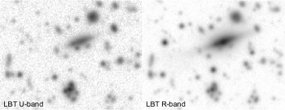
    Figure 23: Galaxy 25 (top): An assembly type system with two diffuse bridges linking two brighter clump cores. All except the bridge on the left connecting the two cores are detected in both $r$-band and U-band. Galaxy 26 (bottom): An edge-on spiral galaxy with extended flux toward the left seen in the $r$-band , but not in the U-band. At the bottom of the image, there is a galaxy consisting of several clumps.

27. An edge-on spiral galaxy with extended flux on the left side, which is only detected in the $r$-band (bottom galaxy in Fig. 23). There are other galaxies in the image with irregular shapes, and signatures of recent interactions or mergers, including a galaxy consisting of clumps at the bottom of the image. There is no redshift information available for any of the objects in the image.

    

     

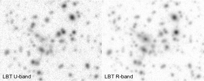
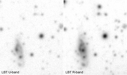
    Figure 24: Galaxy 27 (top): A dense area with multiple galaxies interacting and a clear tidal stream between two galaxies near center. Most of the galaxies and features within the field are detected in both $r$-band and U-band. The QSO in the system has a $z_{spec}$ = 0.334. Galaxy 28 (bottom): A system in the process of merging with potential double nuclei and a diffuse stream toward the top of the image. In the U-band, the central nucleus is not visible.

28. A dense area of galaxies with multiple possible interactions (top system of galaxies in Fig. 24). The most obvious one is a bridge between two galaxies near the center and is visible in both the $r$-band and the $U$-band. There is also a known QSO in the field with a $z_{spec}$ = 0.334 (Albareti et al., 2017). The remainder of the objects in the field do not have known redshifts.

29. A potential double nuclei merging system with diffuse flux above the galaxy in $r$-band (bottom galaxy in fig. 24). While most of the galaxy is detected in U-band, remarkably, the bright core in the center not visible in the U-band. Visually there appears to be links to nearby objects, but there is no redshift information to confirm.

30. An elliptical galaxy with diffuse plumes seen in the $r$-band , but in the U-band the plumes are less distinct (top galaxy in Fig. 25). There is no redshift information for this galaxy.

    

     

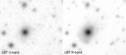
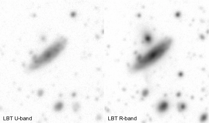
    Figure 25: Galaxy 29 (top): An interesting extended plume of diffuse light toward the bottom left seen only in the $r$-band. Galaxy 30 (bottom): An angled spiral galaxy, with a tidal bridge extending down toward the smaller galaxy below it, which is not detected in the U-band.

31. An angled spiral galaxy with diffuse flux extending down toward the smaller galaxy below it (bottom galaxy in Fig. 25). The possible diffuse bridge linking the two galaxies is only detected in the $r$-band. However, without redshift information, it is not possible to know for sure if these objects are truly interacting.

References

- Adams et al. (2022) Adams, D., Mehta, V., Dickinson, H., et al. 2022, ApJ, 931, 16, doi: 10.3847/1538-4357/ac6512
- Ahumada et al. (2020) Ahumada, R., Prieto, C. A., Almeida, A., et al. 2020, ApJS, 249, 3, doi: 10.3847/1538-4365/ab929e
- Albareti et al. (2017) Albareti, F. D., Allende Prieto, C., Almeida, A., et al. 2017, ApJS, 233, 25, doi: 10.3847/1538-4365/aa8992
- Andrews et al. (2018) Andrews, S. K., Driver, S. P., Davies, L. J. M., Lagos, C. d. P., & Robotham, A. S. G. 2018, MNRAS, 474, 898, doi: 10.1093/mnras/stx2843
- Ashcraft et al. (2018) Ashcraft, T. A., Windhorst, R. A., Jansen, R. A., et al. 2018, PASP, 130, 064102, doi: 10.1088/1538-3873/aab542
- Barger et al. (2002) Barger, A. J., Cowie, L. L., Brandt, W. N., et al. 2002, AJ, 124, 1839, doi: 10.1086/342448
- Barger et al. (2008) Barger, A. J., Cowie, L. L., & Wang, W. H. 2008, ApJ, 689, 687, doi: 10.1086/592735
- Barnes (1992) Barnes, J. E. 1992, ApJ, 393, 484, doi: 10.1086/171522
- Beckwith et al. (2006) Beckwith, S. V. W., Stiavelli, M., Koekemoer, A. M., et al. 2006, AJ, 132, 1729, doi: 10.1086/507302
- Bertin & Arnouts (1996) Bertin, E., & Arnouts, S. 1996, A&AS, 117, 393, doi: 10.1051/aas:1996164
- Bertin & Amorisco (2010) Bertin, G., & Amorisco, N. C. 2010, A&A, 512, A17, doi: 10.1051/0004-6361/200913611
- Bertin et al. (2002) Bertin, G., Ciotti, L., & Del Principe, M. 2002, A&A, 386, 149, doi: 10.1051/0004-6361:20020248
- Biggs & Ivison (2006) Biggs, A. D., & Ivison, R. J. 2006, MNRAS, 371, 963, doi: 10.1111/j.1365-2966.2006.10730.x
- Blanton et al. (2017) Blanton, M. R., Bershady, M. A., Abolfathi, B., et al. 2017, AJ, 154, 28, doi: 10.3847/1538-3881/aa7567
- Bundy et al. (2005) Bundy, K., Ellis, R. S., & Conselice, C. J. 2005, ApJ, 625, 621, doi: 10.1086/429549
- Burkey et al. (1994) Burkey, J. M., Keel, W. C., Windhorst, R. A., & Franklin, B. E. 1994, ApJ, 429, L13, doi: 10.1086/187402
- Carleton et al. (2022) Carleton, T., Windhorst, R. A., O’Brien, R., et al. 2022, arXiv e-prints, arXiv:2205.06347. https://arxiv.org/abs/2205.06347
- Casey et al. (2012) Casey, C. M., Berta, S., Béthermin, M., et al. 2012, ApJ, 761, 140, doi: 10.1088/0004-637X/761/2/140
- Conselice (2014) Conselice, C. J. 2014, ARA&A, 52, 291, doi: 10.1146/annurev-astro-081913-040037
- Darg et al. (2010) Darg, D. W., Kaviraj, S., Lintott, C. J., et al. 2010, MNRAS, 401, 1043, doi: 10.1111/j.1365-2966.2009.15686.x
- Driver & Robotham (2010) Driver, S. P., & Robotham, A. S. G. 2010, MNRAS, 407, 2131, doi: 10.1111/j.1365-2966.2010.17028.x
- Driver et al. (2011) Driver, S. P., Hill, D. T., Kelvin, L. S., et al. 2011, MNRAS, 413, 971, doi: 10.1111/j.1365-2966.2010.18188.x
- Driver et al. (2016) Driver, S. P., Andrews, S. K., Davies, L. J., et al. 2016, ApJ, 827, 108, doi: 10.3847/0004-637X/827/2/108
- Duncan et al. (2019) Duncan, K., Conselice, C. J., Mundy, C., et al. 2019, ApJ, 876, 110, doi: 10.3847/1538-4357/ab148a
- Elmegreen et al. (2009a) Elmegreen, B. G., Elmegreen, D. M., Fernandez, M. X., & Lemonias, J. J. 2009a, ApJ, 692, 12, doi: 10.1088/0004-637X/692/1/12
- Elmegreen et al. (2009b) Elmegreen, B. G., Galliano, E., & Alloin, D. 2009b, ApJ, 703, 1297, doi: 10.1088/0004-637X/703/2/1297
- Elmegreen et al. (2007) Elmegreen, D. M., Elmegreen, B. G., Ferguson, T., & Mullan, B. 2007, ApJ, 663, 734, doi: 10.1086/518715
- Elmegreen et al. (2021) Elmegreen, D. M., Elmegreen, B. G., Whitmore, B. C., et al. 2021, ApJ, 908, 121, doi: 10.3847/1538-4357/abd541
- Fisher et al. (2014) Fisher, D. B., Glazebrook, K., Bolatto, A., et al. 2014, ApJ, 790, L30, doi: 10.1088/2041-8205/790/2/L30
- Giallongo et al. (2008) Giallongo, E., Ragazzoni, R., Grazian, A., et al. 2008, A&A, 482, 349, doi: 10.1051/0004-6361:20078402
- Giavalisco et al. (2004) Giavalisco, M., Ferguson, H. C., Koekemoer, A. M., et al. 2004, ApJ, 600, L93, doi: 10.1086/379232
- Grogin et al. (2011) Grogin, N. A., Kocevski, D. D., Faber, S. M., et al. 2011, ApJS, 197, 35, doi: 10.1088/0067-0049/197/2/35
- Hauser et al. (1998) Hauser, M. G., Arendt, R. G., Kelsall, T., et al. 1998, ApJ, 508, 25, doi: 10.1086/306379
- Hernquist (1989) Hernquist, L. 1989, Nature, 340, 687, doi: 10.1038/340687a0
- Koekemoer et al. (2011) Koekemoer, A. M., Faber, S. M., Ferguson, H. C., et al. 2011, ApJS, 197, 36, doi: 10.1088/0067-0049/197/2/36
- Korngut et al. (2022) Korngut, P. M., Kim, M. G., Arai, T., et al. 2022, ApJ, 926, 133, doi: 10.3847/1538-4357/ac44ff
- Lauer et al. (2021) Lauer, T. R., Postman, M., Weaver, H. A., et al. 2021, ApJ, 906, 77, doi: 10.3847/1538-4357/abc881
- Lauer et al. (2022) Lauer, T. R., Postman, M., Spencer, J. R., et al. 2022, ApJ, 927, L8, doi: 10.3847/2041-8213/ac573d
- Lotz et al. (2011) Lotz, J. M., Jonsson, P., Cox, T. J., et al. 2011, ApJ, 742, 103, doi: 10.1088/0004-637X/742/2/103
- Lotz et al. (2008) Lotz, J. M., Davis, M., Faber, S. M., et al. 2008, ApJ, 672, 177, doi: 10.1086/523659
- Matsumoto et al. (2018) Matsumoto, T., Tsumura, K., Matsuoka, Y., & Pyo, J. 2018, AJ, 156, 86, doi: 10.3847/1538-3881/aad0f0
- Matsumoto et al. (2005) Matsumoto, T., Matsuura, S., Murakami, H., et al. 2005, ApJ, 626, 31, doi: 10.1086/429383
- Matsumoto et al. (2011) Matsumoto, T., Seo, H. J., Jeong, W. S., et al. 2011, ApJ, 742, 124, doi: 10.1088/0004-637X/742/2/124
- McVittie & Wyatt (1959) McVittie, G. C., & Wyatt, S. P. 1959, ApJ, 130, 1, doi: 10.1086/146688
- Mohamed & Reshetnikov (2011) Mohamed, Y. H., & Reshetnikov, V. P. 2011, Astrophysics, 54, 155, doi: 10.1007/s10511-011-9168-7
- Moran et al. (2007) Moran, S. M., Loh, B. L., Ellis, R. S., et al. 2007, ApJ, 665, 1067, doi: 10.1086/519550
- Morrison et al. (2010) Morrison, G. E., Owen, F. N., Dickinson, M., Ivison, R. J., & Ibar, E. 2010, ApJS, 188, 178, doi: 10.1088/0067-0049/188/1/178
- Oke & Gunn (1983) Oke, J. B., & Gunn, J. E. 1983, ApJ, 266, 713, doi: 10.1086/160817
- Otteson et al. (2021) Otteson, L., McCabe, T., Ashcraft, T. A., et al. 2021, Research Notes of the American Astronomical Society, 5, 190, doi: 10.3847/2515-5172/ac1db6
- Overzier et al. (2009) Overzier, R. A., Heckman, T. M., Tremonti, C., et al. 2009, ApJ, 706, 203, doi: 10.1088/0004-637X/706/1/203
- Puget et al. (1996) Puget, J. L., Abergel, A., Bernard, J. P., et al. 1996, A&A, 308, L5
- Rafferty et al. (2011) Rafferty, D. A., Brandt, W. N., Alexander, D. M., et al. 2011, ApJ, 742, 3, doi: 10.1088/0004-637X/742/1/3
- Redshaw et al. (2022) Redshaw, C., McCabe, T., Otteson, L., et al. 2022, Research Notes of the American Astronomical Society, 6, 63, doi: 10.3847/2515-5172/ac6189
- Rix et al. (2004) Rix, H.-W., Barden, M., Beckwith, S. V. W., et al. 2004, ApJS, 152, 163, doi: 10.1086/420885
- Scoville et al. (2007) Scoville, N., Aussel, H., Brusa, M., et al. 2007, ApJS, 172, 1, doi: 10.1086/516585
- Straughn et al. (2006) Straughn, A. N., Cohen, S. H., Ryan, R. E., et al. 2006, ApJ, 639, 724, doi: 10.1086/499576
- Straughn et al. (2015) Straughn, A. N., Voyer, E. N., Eufrasio, R. T., et al. 2015, ApJ, 814, 97, doi: 10.1088/0004-637X/814/2/97
- Taylor et al. (2004) Taylor, V. A., Jansen, R. A., & Windhorst, R. A. 2004, PASP, 116, 762, doi: 10.1086/422929
- Toomre & Toomre (1972) Toomre, A., & Toomre, J. 1972, ApJ, 178, 623, doi: 10.1086/151823
- Treu et al. (2005) Treu, T., Ellis, R. S., Liao, T. X., & van Dokkum, P. G. 2005, ApJ, 622, L5, doi: 10.1086/429374
- Wang et al. (2016) Wang, S., Liu, J., Qiu, Y., et al. 2016, ApJS, 224, 40, doi: 10.3847/0067-0049/224/2/40
- Wen & Zheng (2016) Wen, Z. Z., & Zheng, X. Z. 2016, ApJ, 832, 90, doi: 10.3847/0004-637X/832/1/90
- Windhorst et al. (2011) Windhorst, R. A., Cohen, S. H., Hathi, N. P., et al. 2011, ApJS, 193, 27, doi: 10.1088/0067-0049/193/2/27
- Windhorst et al. (2018) Windhorst, R. A., Timmes, F. X., Wyithe, J. S. B., et al. 2018, ApJS, 234, 41, doi: 10.3847/1538-4365/aaa760
- Windhorst et al. (2022) Windhorst, R. A., Carleton, T., O’Brien, R., et al. 2022, arXiv e-prints, arXiv:2205.06214. https://arxiv.org/abs/2205.06214
- Wirth et al. (2004) Wirth, G. D., Willmer, C. N. A., Amico, P., et al. 2004, AJ, 127, 3121, doi: 10.1086/420999