Truncated Matrix Power Iteration for
Differentiable DAG Learning

Abstract

Recovering underlying Directed Acyclic Graph (DAG) structures from observational data is highly challenging due to the combinatorial nature of the DAG-constrained optimization problem. Recently, DAG learning has been cast as a continuous optimization problem by characterizing the DAG constraint as a smooth equality one, generally based on polynomials over adjacency matrices. Existing methods place very small coefficients on high-order polynomial terms for stabilization, since they argue that large coefficients on the higher-order terms are harmful due to numeric exploding. On the contrary, we discover that large coefficients on higher-order terms are beneficial for DAG learning, when the spectral radiuses of the adjacency matrices are small, and that larger coefficients for higher-order terms can approximate the DAG constraints much better than the small counterparts. Based on this, we propose a novel DAG learning method with efficient truncated matrix power iteration to approximate geometric series based DAG constraints. Empirically, our DAG learning method outperforms the previous state-of-the-arts in various settings, often by a factor of $3$ or more in terms of structural Hamming distance.

1 Introduction

Recovery of Directed Acyclic Graphs (DAGs) from observational data is a classical problem in many fields, including bioinformatics [31, 49], machine learning [19], and causal inference [39]. The graphical model produced by a DAG learning algorithm allows one to decompose the joint distribution over the variables of interest in a compact and flexible manner, and under certain assumptions [27, 39], these graphical models can have causal interpretations.

DAG learning methods can be roughly categorized into constraint-based and score-based methods. Most constraint-based approaches, e.g., PC [37], FCI [38, 11], rely on conditional independence test and thus may require a large sample size [33, 43]. The score-based approaches, including exact methods based on dynamic programming [18, 36, 35], A* search [48, 47], and integer programming [13], as well as greedy methods like GES [9], model the validity of a graph according to some score function and are often formulated and solved as a discrete optimization problem. A key challenge for score-based methods is the combinatorial search space of DAGs [8, 10].

There is a recent interest in developing continuous optimization methods for DAG learning in the past few years. In particular, Zheng et al. [50] develops an algebraic characterization of DAG constraint based on a continuous function, specifically matrix exponential, of the weighted adjacency matrix of a graph, and applies it to estimate linear DAGs with equal noise variances using continuous constrained optimization [4, 5]. The resulting algorithm is called NOTEARS. Yu et al. [45] proposes an alternative DAG constraint based on powers of a binomial to improve practical convenience. Wei et al. [44] unifies these two DAG constraints by writing them in terms of a general polynomial one. These DAG constraints have been applied to more complex settings, e.g., with nonlinear relationships [45, 51, 20, 25], time series [26], confounders [6], and flexible score functions [53], and have been shown to produce competitive performance. Apart from the polynomial based constraints, Lee et al. [21], Zhu et al. [52] present alternative formulations of the DAG constraints based on the spectral radius of the weighted adjacency matrix. Instead of solving a constrained optimization problem, Yu et al. [46] proposes NOCURL which employs an algebraic representation of DAGs such that continuous unconstrained optimization can be carried out in the DAG space directly. However, the focus of these works [21, 52, 46] is to improve the scalability, and the performance of the resulting methods may degrade.

To avoid potential numeric exploding that may be caused by high-order terms in the polynomial-based DAG constraints, previous works use very small coefficients for high-order terms in DAG constraints [50, 45]. More precisely, the coefficients decrease quickly to very small values for the relatively higher order terms that may contain useful higher-order information. This may cause difficulties for the DAG constraints to capture the higher-order information for enforcing acyclicity. With such DAG constraints, a possible solution to maintain higher-order information for acyclicity is to apply an even larger penalty weight [50, 45], which, however, causes ill-conditioning issues as demonstrated by Ng et al. [24]. Moreover, these small coefficients will be multiplied on the gradients of higher-order terms during the optimization process, leading to gradient vanishing. In this paper, we show that, on the contrary, larger coefficients may be safely used to construct more informative higher-order terms without introducing numeric exploding. The reason is that the weighted adjacency matrix of a DAG must be nilpotent; thus the candidate adjacency matrix often has a very small spectral radius. As a result, the higher-order power of the matrix may be very close to zero matrix, and larger coefficients may be safely used without causing numeric exploding. We thus propose to use geometric series-based DAG constraint without small coefficients for more accurate and robust DAG learning. To relieve the computational burden from the geometric series, we propose an efficient Truncated Matrix Power Iteration (TMPI) algorithm with a theoretically guaranteed error bound. We summarize our contributions as the following:

• We demonstrate that the key challenge for DAG learning is the gradient vanishing issue instead of gradient and numeric exploding. For sparse graphs, the gradient vanishing issue can be severe.

• We design a DAG constraint based on finite geometric series which is an order-$d$ polynomial over adjacency matrices to escape from gradient vanishing. We show that the relatively large coefficients on the higher-order terms would not result in gradient exploding in practice.

• We show that there exists some constant $k\leqslant d$, s.t. our order-$d$ polynomial constraint can be reduced to order-$k$ polynomial without expanding its feasible set. Though finding such value of $k$ requires solving the NP-hard longest simple path problem, we develop a simple heuristic to find such $k$ with bounded error to the exact, order-$d$, DAG constraint. Based on this result, we propose a DAG constraint based on efficient Truncated Matrix Power Iteration (TMPI), and conduct experiments to demonstrate that the resulting DAG learning method outperforms previous methods by a large margin.

• We provide a systematical empirical comparison of the existing DAG constraints, including the polynomial and spectral radius based constraints, as well as the algebraic DAG representation of NOCURL.

2 Preliminaries

DAG Model and Linear SEM

Given a DAG model (a.k.a. Bayesian network) defined over random vector $\operatorname{\mathbf{x}}=[x_{1},x_{2},\ldots,x_{d}]^{\top}$ and DAG $\mathcal{G}$, the distribution $P(\operatorname{\mathbf{x}})$ and DAG $\mathcal{G}$ are assumed to satisfy the Markov assumption [39, 27]. We say that $\operatorname{\mathbf{x}}$ follows a linear Structural Equation Model (SEM) if

$$\operatorname{\mathbf{x}}=\operatorname{\mathbf{B}}^{\top}\operatorname{\mathbf{x}}+\operatorname{\mathbf{e}},$$ (1)

where $\operatorname{\mathbf{B}}$ is the weighted adjacency matrix representing the DAG $\mathcal{G}$, and $\operatorname{\mathbf{e}}=[e_{1},e_{2},\ldots,e_{d}]^{\top}$ denotes the exogenous noise vector consisting of $d$ independent random variables. With slight abuse of notation, we denote by $\mathcal{G}(\operatorname{\mathbf{B}})$ the graph induced by weighted adjacency matrix $\operatorname{\mathbf{B}}$. Moreover, we do not distinguish between random variables and vertices or nodes, and use these terms interchangeably.

Our goal is to estimate the DAG $\operatorname{\mathcal{G}}$ from $n$ i.i.d. samples of $\operatorname{\mathbf{x}}$, indicated by the matrix $\operatorname{\mathbf{X}}\in\mathbb{R}^{n\times d}$. In general, the DAG $\mathcal{G}$ can only be identified up to its Markov equivalence class under the faithfulness [39] or sparsest Markov representation [30] assumption. It has been shown that for linear SEMs with homoscedastic errors, from which the noise terms are specified up to a constant [22], and for linear non-Gaussian SEMs, from which no more than one of the noise term is Gaussian [34], the true DAG can be fully identified. In this work, we focus on the linear SEMs with equal noise variances [28], which can be viewed as an instance of the former.

DAG Constraints for Differentiable DAG Learning

Recently, Zheng et al. [50] reformulated the DAG learning problem as the following continuous optimization problem with convex least-squares objective but non-convex constraint,

$$\min_{\operatorname{\mathbf{B}}\in\mathbb{R}^{d\times d}}\ \ \|\operatorname{\mathbf{X}}-\operatorname{\mathbf{X}}\operatorname{\mathbf{B}}\|_{F}^{2}+\eta\|\operatorname{\mathbf{B}}\|_{1},\quad\text{subject\leavevmode\nobreak\ to}\leavevmode\nobreak\ h_{\text{exp}}(\operatorname{\mathbf{B}}\odot\operatorname{\mathbf{B}})=0,$$ (2)

where $\|\cdot\|_{F}$ and $\|\cdot\|_{1}$ denote the Frobenius norm and elementwise $\ell_{1}$ norm, respectively, $\eta>0$ is the regularization coefficient that controls the sparsity of $\operatorname{\mathbf{B}}$, and $\odot$ denotes the Hadamard product, which is used to map $\operatorname{\mathbf{B}}$ to a positive weighted adjacency matrix with the same structure. Given any $\tilde{\operatorname{\mathbf{B}}}\in\mathbb{R}_{\geqslant 0}^{d\times d}$, the function $h_{\text{exp}}$ is defined as

$$h_{\text{exp}}(\tilde{\operatorname{\mathbf{B}}})=\mathrm{tr}(e^{\tilde{\operatorname{\mathbf{B}}}})-d=\mathrm{tr}\left(\sum_{i=1}^{\infty}\frac{1}{i!}\tilde{\operatorname{\mathbf{B}}}^{i}\right),$$ (3)

and can be efficiently computed using various approaches [1, 2]. The key here is that $h_{\text{exp}}(\tilde{\operatorname{\mathbf{B}}})=0$ if and only if $\operatorname{\mathcal{G}}(\tilde{\operatorname{\mathbf{B}}})$ is a DAG. The formulation (2) involves a hard constraint, and Zheng et al. [50] adopted the augmented Lagrangian method [4, 5] to solve the constrained optimization problem. Ng et al. [24] demonstrated that the augmented Lagrangian method here behaves similarly to the classical quadratic penalty method [29, 15] in practice, and showed that it is guaranteed to return a DAG under certain conditions.

To improve practical convenience, Yu et al. [45] proposed a similar DAG constraint using an order-$d$ polynomial based on powers of a binomial, given by

$$h_{\text{bin}}(\tilde{\operatorname{\mathbf{B}}})=\mathrm{tr}\left(\mathbb{I}+\alpha\tilde{\operatorname{\mathbf{B}}}\right)^{d}{{-d}}=\mathrm{tr}\left(\sum_{i=1}^{d}{d\choose i}\alpha^{i}\tilde{\operatorname{\mathbf{B}}}^{i}\right),$$ (4)

where $\alpha>0$ is a hyperparameter and is often set to $1/d$, e.g., in the implementation of DAG-GNN [45]. This function can be evaluated using $O(\log d)$ matrix multiplications using the exponentiation by squaring algorithm. Both $h_{\text{exp}}(\tilde{\operatorname{\mathbf{B}}})$ and $h_{\text{bin}}(\tilde{\operatorname{\mathbf{B}}})$ are formulated by Wei et al. [44] as a unified one

$$h_{\text{poly}}(\tilde{\operatorname{\mathbf{B}}})=\mathrm{tr}\left(\sum_{i=1}^{d}c_{i}\tilde{\operatorname{\mathbf{B}}}^{i}\right),\quad c_{i}>0,\quad i=1,2,\dots,d.$$ (5)

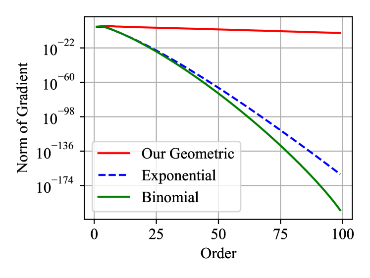
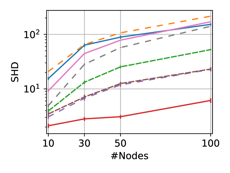
Figure 1: Previous polynomial based DAG constraints, including exponential (Eq. (3)) and binomial (Eq. (4) with $\alpha=1/d$) constraints, suffer from gradient vanishing. Left: The norm of gradient on higher-order terms w.r.t. order on a $100$-node graph generated using the ER2 setting in Section 4. Note that the gradients on different order terms refer to $\nabla_{\tilde{\mathbf{B}}}c_{i}\operatorname{tr}(\tilde{\mathbf{B}}^{i})$, where, for different polynomial based DAG constraints, the coefficients $c_{i}$ are different. Right: We propose a geometric series based DAG constraint, named Truncated Matrix Power Iteration (TMPI), to escape from vanished gradients, which leads to a significant performance improvement in terms of Structural Hamming Distance (SHD) on ER2 graphs (see Section 4 for full experimental details and results).

3 DAG Learning with Truncated Matrix Power Iteration

In this section, we first show that gradient vanishing is one main issue for previous DAG constraints and propose a truncated geometric series based DAG constraints to escape from the issue in Section 3.1. Then in Section 3.2 the theoretical properties of our DAG constraints are analyzed. In Section 3.3 we provide an efficient algorithm for our DAG constraints. In Section 3.4, we discuss the relation between our algorithm and previous works.

3.1 Gradient Vanishing Issue and Truncated Geometric DAG Constraint

Theoretically, any positive values of $c_{i}$ suffice to make the DAG constraint term $h_{\text{poly}}(\tilde{\operatorname{\mathbf{B}}})$ in Eq. (5) a valid one, i.e., it equals zero if and only if the graph $\operatorname{\mathcal{G}}(\tilde{\operatorname{\mathbf{B}}})$ is acyclic. Thus previously small coefficients for higher-order terms are preferred since they are known to have better resistance to numeric exploding of higher-order polynomials [50, 45]. These small coefficients forbid informative higher-order terms and cause severe gradient vanishing, as nilpotent properties of DAG result in candidate adjacency matrix with very small spectral radius (see empirical analysis in Figure 1 left). In this case, the weight updates during the optimization process can hardly utilize this higher-order information from the vanishingly small gradients. As a consequence, only lower-order information can be effectively captured, which may be detrimental to the quality of final solution.

To avoid the severe vanishing gradient issue in existing DAG constraints (e.g., Eq. (3), (4)), we propose to discard the coefficients and use a finite geometric series based function:

$$h_{\text{geo}}(\tilde{\operatorname{\mathbf{B}}}) =\mathrm{tr}\left(\sum_{i=1}^{d}\tilde{\operatorname{\mathbf{B}}}^{i}\right),$$ (6a)

$$\nabla_{\tilde{\operatorname{\mathbf{B}}}}h_{\text{geo}}(\tilde{\operatorname{\mathbf{B}}}) =\left(\sum_{i=0}^{d-1}(i+1)\tilde{\operatorname{\mathbf{B}}}^{i}\right)^{\top}.$$ (6b)

The gradient of $h_{\text{geo}}$ w.r.t. $\tilde{\operatorname{\mathbf{B}}}$ denoted by $\nabla_{\tilde{\operatorname{\mathbf{B}}}}h_{\text{geo}}(\tilde{\operatorname{\mathbf{B}}})$ is an order-$(d-1)$ polynomial of $\tilde{\operatorname{\mathbf{B}}}$.

Compared to (3) and (4), Eq. (6a) is a more precise DAG constraint escaped from from severe gradient vanishing. Also it is notable that due to the nilpotent properties of weighted adjacency matrices of DAGs, the higher-order terms in (6a) and (6b) often comes with small norms; thus, our DAG constraint may not suffer from numeric exploding in practice, based on the observations in Section 4.

In Figure 1 we compared the norm of gradients on higher-order terms of different DAG constraints, where we observe that for previous exponential-based (3) and binomial-based (4) DAG constraints, the gradients of higher-order terms converges to $0$ very quickly as the order increases. Meanwhile, the gradient of higher-order terms in (6a) converges to $0$ with a much slower speed and thus informative higher-order terms are preserved.

We further show that those non-informative higher-order terms that are close to zero in (6a) can be safely dropped to form a more efficient DAG constraint with some $k\leqslant d$, where we often have $k\ll d$ in practice:

$$h_{\text{trunc}}^{k}(\tilde{\operatorname{\mathbf{B}}})=\mathrm{tr}\left(\sum_{i=1}^{k}\tilde{\operatorname{\mathbf{B}}}^{i}\right).$$ (7)

Naively, the DAG constraint (7) requires $\operatorname{\mathcal{O}}(k)$ matrix multiplication which is far less than $\operatorname{\mathcal{O}}(d)$ for (6a), and under mild conditions the error of (7) is tightly bounded (see Proposition 3 for details). In Figure 1 right we show that our DAG constraint (7) (named TMPI) attains far better performance than previous ones as it escapes from gradient vanishing.

3.2 Theoretical Properties of Truncated Geometric DAG Constraint

We analyze the properties of the power of adjacency matrices, which play an important role in constructing DAG constraints. First notice that, for the $k^{\text{th}}$ power of an adjacency matrix $\tilde{\operatorname{\mathbf{B}}}\in\mathbb{R}_{\geqslant 0}^{d\times d}$, its entry $(\tilde{\operatorname{\mathbf{B}}}^{k})_{ij}$ is nonzero if and only if there is a length-$k$ path (not necessarily simple) from node $X_{i}$ to node $X_{j}$ in graph $\operatorname{\mathcal{G}}(\tilde{\operatorname{\mathbf{B}}})$. This straightforwardly leads to the following property, which is a corollary of [44, Lemma 1].

Proposition 1.

Let $\tilde{\operatorname{\mathbf{B}}}\in\mathbb{R}_{\geqslant 0}^{d\times d}$ be the weighted adjacency matrix of a graph $\operatorname{\mathcal{G}}$ with $d$ vertices. $\operatorname{\mathcal{G}}$ is a DAG if and only if $\tilde{\operatorname{\mathbf{B}}}^{d}=\mathbf{0}$.

Proposition 1 can be used to construct a single-term DAG constraint term, given by

$$h_{\text{single}}(\tilde{\operatorname{\mathbf{B}}})=\|\tilde{\operatorname{\mathbf{B}}}^{d}\|_{p},$$ (8)

where $\|\cdot\|_{p}$ denotes an elementwise $\ell_{p}$ norm. However, as the candidate adjacency matrix gets closer to acyclic, the spectral radius of $\tilde{\operatorname{\mathbf{B}}}^{d}$ will become very small. As a result, the value $h_{\text{single}}(\tilde{\operatorname{\mathbf{B}}})$, as well as its gradient $\nabla_{\tilde{\operatorname{\mathbf{B}}}}h_{\text{single}}(\tilde{\operatorname{\mathbf{B}}})$ may become too small to be represented in limited machine precision. This suggests the use of the polynomial based constraints for better performance.

Without any prior information of the graph, one has to compute the $d^{\text{th}}$ power of matrix $\tilde{\operatorname{\mathbf{B}}}$, either using the DAG constraint terms in Eq. (8) or (5). However, if the length of the longest simple path in the graph is known, we can formulate a lower-order polynomial based DAG constraint.

Proposition 2.

Let $\tilde{\operatorname{\mathbf{B}}}\in\mathbb{R}_{\geqslant 0}^{d\times d}$ be the weighted adjacency matrix of a graph $\operatorname{\mathcal{G}}$ with $d$ vertices, and $k$ be the length of the longest simple path in graph $\operatorname{\mathcal{G}}$. The following three conditions are equivalent: (1) $\operatorname{\mathcal{G}}$ is a DAG, (2) $\tilde{\operatorname{\mathbf{B}}}^{k+1}=0$, and (3) $h_{\text{trunc}}^{k}(\tilde{\operatorname{\mathbf{B}}})=0$.

The intuition of the above proposition is as follows. For the graph whose largest simple cycle has a length of $k$, it suffices to compute the $k^{\text{th}}$ power of its adjacency matrix, since computing any power larger than $k$ is simply traveling in the cycles repeatedly. Therefore, Proposition 2 suggests that $h_{\text{trunc}}^{k}(\tilde{\operatorname{\mathbf{B}}})=0$ is a valid DAG constraint.

Unfortunately, the longest simple path problem for general graphs is known to be NP-hard [32], and thus we have to find an alternative way to seek the proper $k$. For a candidate adjacency matrix $\tilde{\operatorname{\mathbf{B}}}$, a simple heuristic is to iterate over the power of matrices to find some $k$ s.t. matrix $\tilde{\operatorname{\mathbf{B}}}^{k}$ is close enough to a zero matrix. Recall that Proposition 1 implies that the adjacency matrix of a DAG is nilpotent; therefore, when a candidate adjacency matrix $\tilde{\operatorname{\mathbf{B}}}$ is close to being acyclic, its spectral radius would be close to zero, which implies that the $\tilde{\operatorname{\mathbf{B}}}^{k}$ would converge quickly to zero as $k$ increases. Thus, if we use the above heuristic to find $k$, it is highly possible that we find some $k\ll d$.

By using an approximate $k$ instead of the exact one, the DAG constraint in Eq. (7) becomes an approximate one with the following bounds. Denoting by $\|\cdot\|_{\infty}$ the elementwise infinity norm (i.e., maximum norm), we have the following proposition.

Proposition 3.

Given $\tilde{\operatorname{\mathbf{B}}}\in\mathbb{R}_{\geqslant 0}^{d\times d}$, if there exists $k<d$ such that $\|\tilde{\operatorname{\mathbf{B}}}^{k}\|_{\infty}\leqslant\epsilon<\frac{1}{(k+1)d}$, then we have

$$\begin{split}&0\leqslant h_{\text{geo}}(\tilde{\operatorname{\mathbf{B}}})-h_{\text{trunc}}^{k}(\tilde{\operatorname{\mathbf{B}}})\leqslant\frac{1-(d\epsilon)^{{d/k-1}}}{1-(d\epsilon)^{1/k}}d^{2+1/k}\epsilon^{1+1/k},\\ &0\leqslant\|\nabla_{\tilde{\operatorname{\mathbf{B}}}}h_{\text{geo}}(\tilde{\operatorname{\mathbf{B}}})-\nabla_{\tilde{\operatorname{\mathbf{B}}}}h_{\text{trunc}}^{k}(\tilde{\operatorname{\mathbf{B}}})\|_{F}\leqslant(k+1)d\epsilon\|\nabla_{\tilde{\operatorname{\mathbf{B}}}}h_{\text{geo}}(\tilde{\operatorname{\mathbf{B}}})\|_{F}.\end{split}$$

Remark 1.

The condition $\epsilon<\frac{1}{(k+1)d}$ in the proposition above is such that the inequalities are non-vacuous, specifically since we must have $\|\nabla_{\tilde{\operatorname{\mathbf{B}}}}h_{\text{geo}}(\tilde{\operatorname{\mathbf{B}}})-\nabla_{\tilde{\operatorname{\mathbf{B}}}}h_{\text{trunc}}^{k}(\tilde{\operatorname{\mathbf{B}}})\|_{F}/\|\nabla_{\tilde{\operatorname{\mathbf{B}}}}h_{\text{geo}}(\tilde{\operatorname{\mathbf{B}}})\|_{F}<1$.

Proposition 3 provides an efficient way to bound the error of truncated constraints $h_{\text{trunc}}^{k}(\tilde{\operatorname{\mathbf{B}}})$ to the geometric series based DAG constraints $h_{\text{geo}}(\tilde{\operatorname{\mathbf{B}}})$. However, it also demonstrates a possible limitation for all polynomial based DAG constraints. As we know, when a solution is close to DAG, its spectral radius will be close to zero. In this situation, if the longest simple path in a graph is long, it is unavoidable to use high-order terms to capture this information while such high-order terms might be close to $0$. In the worst case, the higher-order terms may underflow due to limited machine precision. Thus some specific numerically stable method may be required, and we leave this for future work.

3.3 Dynamic Truncated Matrix Power Iteration

Proposition 3 indicates that it may be safe to discard those matrix powers with index larger than $k$. In this case, the DAG constraint and its gradient correspond to order-$k$ and order-$(k-1)$ polynomials of $\tilde{\operatorname{\mathbf{B}}}$, respectively. A straightforward way to compute the DAG constraint as well as the gradient is provided in Algorithm 1, which we call TMPI. The general polynomial based DAG constraint in (5) requires $\operatorname{\mathcal{O}}(d)$ matrix multiplication, while Algorithm 1 reduces the number of multiplication to $\operatorname{\mathcal{O}}(k)$. In practice, $k$ can be much smaller than $d$; for example, when recovering $100$-node Erdős–Rényi DAG with expected degree $4$, $k$ is often smaller than $20$.

Algorithm 1 Truncated Matrix Power Iteration (TMPI)

Input: $\tilde{\operatorname{\mathbf{B}}}\in\mathbb{R}_{\geqslant 0}^{d\times d}$, $\epsilon$
Output: $h(\tilde{\operatorname{\mathbf{B}}})$, $\nabla_{\tilde{\operatorname{\mathbf{B}}}}h(\tilde{\operatorname{\mathbf{B}}})$

1:  $i\leftarrow 2,h(\tilde{\operatorname{\mathbf{B}}})\leftarrow\mathrm{tr}(\tilde{\operatorname{\mathbf{B}}})$, $\nabla_{\tilde{\operatorname{\mathbf{B}}}}h(\tilde{\operatorname{\mathbf{B}}})\leftarrow\mathbb{I}$

2:  while $i\leqslant d$ do

3:    $\nabla_{\tilde{\operatorname{\mathbf{B}}}}h(\tilde{\operatorname{\mathbf{B}}})\leftarrow\nabla_{\tilde{\operatorname{\mathbf{B}}}}h(\tilde{\operatorname{\mathbf{B}}})+i(\tilde{\operatorname{\mathbf{B}}}^{i-1})^{\top}$

4:    $\tilde{\operatorname{\mathbf{B}}}^{i}\leftarrow\tilde{\operatorname{\mathbf{B}}}\tilde{\operatorname{\mathbf{B}}}^{i-1}$

5:    $h(\tilde{\operatorname{\mathbf{B}}})\leftarrow h(\tilde{\operatorname{\mathbf{B}}})+\mathrm{tr}(\tilde{\operatorname{\mathbf{B}}}^{i})$

6:    if $\|\tilde{\operatorname{\mathbf{B}}}^{i}\|_{\infty}\leqslant\epsilon$ then break

7:    $i\leftarrow i+1$

8:  end while

9:  Output $h(\tilde{\operatorname{\mathbf{B}}})$, $\nabla_{\tilde{\operatorname{\mathbf{B}}}}h(\tilde{\operatorname{\mathbf{B}}})$

Algorithm 2 Fast TMPI

Input: $\tilde{\operatorname{\mathbf{B}}}\in\mathbb{R}_{\geqslant 0}^{d\times d}$, $\epsilon$
Output: $h(\tilde{\operatorname{\mathbf{B}}}),\nabla_{\tilde{\operatorname{\mathbf{B}}}}h(\tilde{\operatorname{\mathbf{B}}})$

1:  $i\leftarrow 1$

2:  $\tilde{\operatorname{\mathbf{B}}}_{f}\leftarrow\tilde{\operatorname{\mathbf{B}}},\tilde{\operatorname{\mathbf{B}}}_{g}\leftarrow\mathbb{I},\tilde{\operatorname{\mathbf{B}}}_{p}\leftarrow\tilde{\operatorname{\mathbf{B}}}$ {$\tilde{\operatorname{\mathbf{B}}}_{f}$ stores $f_{i}(\tilde{\operatorname{\mathbf{B}}})$, $\tilde{\operatorname{\mathbf{B}}}_{g}$ stores $\nabla_{\tilde{\operatorname{\mathbf{B}}}}\mathrm{tr}(f_{i}(\tilde{\operatorname{\mathbf{B}}}))$, and $\tilde{\operatorname{\mathbf{B}}}_{p}$ stores $\tilde{\operatorname{\mathbf{B}}}^{i}$}

3:  while $i\leqslant d$ do

4:    $\tilde{\operatorname{\mathbf{B}}}_{f}^{old}\leftarrow\tilde{\operatorname{\mathbf{B}}}_{f},\tilde{\operatorname{\mathbf{B}}}_{g}^{old}\leftarrow\tilde{\operatorname{\mathbf{B}}}_{g},\tilde{\operatorname{\mathbf{B}}}_{p}^{old}\leftarrow\tilde{\operatorname{\mathbf{B}}}_{p}$

5:    $\tilde{\operatorname{\mathbf{B}}}_{f}\leftarrow\tilde{\operatorname{\mathbf{B}}}_{f}^{old}+\tilde{\operatorname{\mathbf{B}}}_{p}^{old}\tilde{\operatorname{\mathbf{B}}}_{f}^{old}$, $\tilde{\operatorname{\mathbf{B}}}_{p}\leftarrow\tilde{\operatorname{\mathbf{B}}}_{p}^{old}\tilde{\operatorname{\mathbf{B}}}_{p}^{old}$

6:    $\tilde{\operatorname{\mathbf{B}}}_{g}\leftarrow\tilde{\operatorname{\mathbf{B}}}_{g}^{old}+\tilde{\operatorname{\mathbf{B}}}_{p}^{\top}\tilde{\operatorname{\mathbf{B}}}_{g}^{old}+i(\tilde{\operatorname{\mathbf{B}}}_{f}-\tilde{\operatorname{\mathbf{B}}}_{f}^{old}+\tilde{\operatorname{\mathbf{B}}}_{p}^{old}-\tilde{\operatorname{\mathbf{B}}}_{p})$

7:    if $\|\tilde{\operatorname{\mathbf{B}}}_{p}\|_{\infty}\leqslant\epsilon$ then break

8:    $i\leftarrow 2i$

9:  end while

10:  Output $\mathrm{tr}(\tilde{\operatorname{\mathbf{B}}}_{f}),\tilde{\operatorname{\mathbf{B}}}_{g}$

Fast Truncated Matrix Power Iteration

We exploit the specific structure of geometric series to further accelerate the TMPI algorithm from $\operatorname{\mathcal{O}}(k)$ to $\operatorname{\mathcal{O}}(\log k)$ matrix multiplications. This is acheived by leveraging the following recurrence relations, with a proof provided in Appendix A.4.

Proposition 4.

Given any $d\times d$ real matrix $\tilde{\operatorname{\mathbf{B}}}$, let $f_{i}(\tilde{\operatorname{\mathbf{B}}})=\tilde{\operatorname{\mathbf{B}}}+\tilde{\operatorname{\mathbf{B}}}^{2}+\dots+\tilde{\operatorname{\mathbf{B}}}^{i}$ and $h_{i}(\tilde{\operatorname{\mathbf{B}}})=\mathrm{tr}(f_{i}(\tilde{\operatorname{\mathbf{B}}}))$. Then we have the following recurrence relations:

$$f_{i+j}(\tilde{\operatorname{\mathbf{B}}})= f_{i}(\tilde{\operatorname{\mathbf{B}}})+\tilde{\operatorname{\mathbf{B}}}^{i}f_{j}(\tilde{\operatorname{\mathbf{B}}}),$$

$$\nabla_{\tilde{\operatorname{\mathbf{B}}}}h_{i+j}(\tilde{\operatorname{\mathbf{B}}})= \nabla_{\tilde{\operatorname{\mathbf{B}}}}h_{i}(\tilde{\operatorname{\mathbf{B}}})+(\tilde{\operatorname{\mathbf{B}}}^{i})^{\top}\nabla_{\tilde{\operatorname{\mathbf{B}}}}h_{j}(\tilde{\operatorname{\mathbf{B}}})+if_{j}(\tilde{\operatorname{\mathbf{B}}})^{\top}(\tilde{\operatorname{\mathbf{B}}}^{i-1})^{\top}.$$

This straightfowardly implies the following corollary, with a proof given in Appendix A.5.

Corollary 1.

Given any matrix $d\times d$ real matrix $\tilde{\operatorname{\mathbf{B}}}$, let $f_{i}(\tilde{\operatorname{\mathbf{B}}})=\tilde{\operatorname{\mathbf{B}}}+\tilde{\operatorname{\mathbf{B}}}^{2}+\dots+\tilde{\operatorname{\mathbf{B}}}^{i}$ and $h_{i}(\tilde{\operatorname{\mathbf{B}}})=\mathrm{tr}(f_{i}(\tilde{\operatorname{\mathbf{B}}}))$. Then we have have the following recurrence relations:

$$f_{2i}(\tilde{\operatorname{\mathbf{B}}})= (\mathbb{I}+\tilde{\operatorname{\mathbf{B}}}^{i})f_{i}(\tilde{\operatorname{\mathbf{B}}}),$$

$$\nabla_{\tilde{\operatorname{\mathbf{B}}}}h_{2i}(\tilde{\operatorname{\mathbf{B}}})= \nabla_{\tilde{\operatorname{\mathbf{B}}}}h_{i}(\tilde{\operatorname{\mathbf{B}}})+(\tilde{\operatorname{\mathbf{B}}}^{i})^{\top}\nabla_{\tilde{\operatorname{\mathbf{B}}}}h_{i}(\tilde{\operatorname{\mathbf{B}}})+i\left(f_{2i}(\tilde{\operatorname{\mathbf{B}}})-f_{i}(\tilde{\operatorname{\mathbf{B}}})+\tilde{\operatorname{\mathbf{B}}}^{i}-\tilde{\operatorname{\mathbf{B}}}^{2i}\right)^{\top}.$$

Instead of increasing the index $i$ (i.e., power of $\tilde{\operatorname{\mathbf{B}}}$) arithmetically by $1$, as in line $9$ of Algorithm 1, Corollary 1 suggests using its recurrence relations to increase the index $i$ geometrically by a factor of $2$, until the condition $\|\tilde{\operatorname{\mathbf{B}}}^{i}\|_{\infty}\leqslant\epsilon$ is satisfied. The full procedure named Fast TMPI is described in Algorithm 2, which requires $\operatorname{\mathcal{O}}(\log k)$ matrix multiplications and $\operatorname{\mathcal{O}}(d^{2})$ additional storage. An example implementation is given in Listing LABEL:fig:example_impl_fast_tmpi in Appendix B.1. Similar strategy can be applied to the original geometric series based constraint (6a) to form a fast algorithm that requires $\operatorname{\mathcal{O}}(\log d)$ matrix multiplications. A comparison of the time complexity between our proposed constraint and the existing ones is provided in Appendix LABEL:sec:comparison_complexity.

The Full Optimization Framework

For NOTEARS, we apply the same augmented Lagrangian framework [4, 5] adopted by Zheng et al. [50] to convert the constrained optimization problem into the following unconstrained problem

$$\min_{\operatorname{\mathbf{B}}\in\mathbb{R}^{d\times d}}\ \ \|\operatorname{\mathbf{X}}-\operatorname{\mathbf{X}}\operatorname{\mathbf{B}}\|_{F}^{2}+\eta\|\operatorname{\mathbf{B}}\|_{1}+\frac{\rho}{2}h_{\text{trunc}}^{k}(\operatorname{\mathbf{B}}\odot\operatorname{\mathbf{B}})^{2}+\alpha h_{\text{trunc}}^{k}(\operatorname{\mathbf{B}}\odot\operatorname{\mathbf{B}}),$$ (9)

where the parameters $\rho$ and $\alpha$ are iteratively updated using the same strategy as Zheng et al. [50]. We also apply the proposed DAG constraint to GOLEM [23] that adopts likelihood-based objective with soft constraints, leading to the unconstrained optimization problem

$$\min_{\operatorname{\mathbf{B}}\in\mathbb{R}^{d\times d}}\ \ \frac{d}{2}\log\|\operatorname{\mathbf{X}}-\operatorname{\mathbf{X}}\operatorname{\mathbf{B}}\|_{F}^{2}-\log|\det(\mathbb{I}-\operatorname{\mathbf{B}})|+\eta_{1}\|\operatorname{\mathbf{B}}\|_{1}+\eta_{2}h_{\text{trunc}}^{k}(\operatorname{\mathbf{B}}\odot\operatorname{\mathbf{B}}),$$ (10)

where $\eta_{1},\eta_{2}>0$ are the regularization coefficients. In both formulations above, we use Algorithm 1 or 2 to dynamically compute $h_{\text{trunc}}^{k}(\operatorname{\mathbf{B}}\odot\operatorname{\mathbf{B}})$ (and the value of $k$) during each optimization iteration based on a predefined tolerance $\epsilon$.

3.4 Relation to Previous Works

Our algorithm is closely related to the following DAG constraint considered by Zheng et al. [50].

Lemma 1 (Zheng et al. [50, Proposition 1]).

Let $\tilde{\operatorname{\mathbf{B}}}\in\mathbb{R}_{\geqslant 0}^{d\times d}$ with spectral radius smaller than one be the weighted adjacency matrix of a graph $\operatorname{\mathcal{G}}$ with $d$ vertices. $\operatorname{\mathcal{G}}$ is a DAG if and only if

$$\mathrm{tr}(\mathbb{I}-\tilde{\operatorname{\mathbf{B}}})^{-1}=d.$$ (11)

When the spectral radius is smaller than one, the inverse of $\mathbb{I}-\tilde{\operatorname{\mathbf{B}}}$ is simply the following infinite geometric series:

$$(\mathbb{I}-\tilde{\operatorname{\mathbf{B}}})^{-1}=\sum_{i=0}^{\infty}\tilde{\operatorname{\mathbf{B}}}^{i}.$$ (12)

Zheng et al. [50] argued that (12) is not well defined for $\tilde{\operatorname{\mathbf{B}}}$ with spectral radius larger than 1, and in practice the series (12) may explode very quickly. Based on this argument, they adopted the matrix exponential for constructing the DAG constraint. For the same reason, Yu et al. [45] also used very small coefficients for higher-order terms in polynomial based DAG constraints. However, as we illustrate in Section 3, the DAG constraints proposed by Zheng et al. [50], Yu et al. [45] may suffer from gradient vanishing owing to the small coefficients for higher-order terms. In fact, our constraint (7) serves a good approximation for (11) since we are actually looking for an approximate inverse of $\mathbb{I}-\tilde{\operatorname{\mathbf{B}}}$ with a bounded error.

Proposition 5.

Given $\tilde{\operatorname{\mathbf{B}}}\in\mathbb{R}_{\geqslant 0}^{d\times d}$, if there exists $k$ such that $\|\tilde{\operatorname{\mathbf{B}}}^{k}\|_{\infty}\leqslant\epsilon<1/d$, then we have

$$\left\|(\mathbb{I}-\tilde{\operatorname{\mathbf{B}}})^{-1}-\sum_{i=0}^{k}\tilde{\operatorname{\mathbf{B}}}^{k}\right\|_{F}\leqslant d\epsilon\left\|(\mathbb{I}-\tilde{\operatorname{\mathbf{B}}})^{-1}\right\|_{F}.$$

Previous works [44, 24] pointed out that for DAG constraints with form $h(\operatorname{\mathbf{B}}\odot\operatorname{\mathbf{B}})$, the Hadamard product would lead to vanishing gradients in the sense that the gradient $\nabla_{\operatorname{\mathbf{B}}}h(\operatorname{\mathbf{B}}\odot\operatorname{\mathbf{B}})=0$ if and only if $h(\operatorname{\mathbf{B}}\odot\operatorname{\mathbf{B}})=0$. Ng et al. [24] further showed that this may lead to ill-conditioning issue when solving the constrained optimization problem. One may replace the Hadamard product with absolute value, as in Wei et al. [44], but the non-smoothness of absolute value may make the optimization problem difficult to solve and lead to poorer performance [24]. As pointed out by Ng et al. [24], Quasi-Newtown methods, e.g., L-BFGS [7], still perform well even when faced with the ill-conditioning issue caused by vanishing gradients of constraints with form $h(\operatorname{\mathbf{B}}\odot\operatorname{\mathbf{B}})$. In this work, we identify another type of gradient vanishing issue caused by (1) the higher-order terms and small coefficients in function $h$ itself and (2) the small spectral radius of candidate matrix $\operatorname{\mathbf{B}}$, and further provide an effective solution by constructing a Truncated Matrix Power Iteration based DAG constraint.

4 Experiments

We compare the performance of different DAG learning algorithms and DAG constraints to demonstrate the effectiveness of the proposed TMPI based DAG constraint. We provide the main experimental results in this section, and further empirical studies can be found in Appendix LABEL:sec:additional_experiment.

4.1 DAG Learning

We first conduct experiments on synthetic datasets using similar settings as previous works [50, 23, 46]. In summary, random Erdös-Rényi graphs [14] are generated with $d$ nodes and $kd$ expected edges (denoted by ER$k$). Edge weights generated from uniform distribution over the union of two intervals $[-2,-0.5]\cup[0.5,2.0]$ are assigned to each edge to form a weighted adjacency matrix $\operatorname{\mathbf{B}}$. Then $n$ samples are generated from the linear SEM $\operatorname{\mathbf{x}}=\operatorname{\mathbf{B}}\operatorname{\mathbf{x}}+\operatorname{\mathbf{e}}$ to form an $n\times d$ data matrix $\operatorname{\mathbf{X}}$, where the noise $\operatorname{\mathbf{e}}$ are i.i.d. sampled from Gaussian, Exponential, or Gumbel distribution. We set the sample size $n=1000$ and consider $4$ different number of nodes $d=10,30,50,100$ unless otherwise stated. For each setting, we conduct $100$ random simulations to obtain an average performance.

Methods and Baselines

We consider continuous DAG learning methods based on both Mean Squared Error (MSE) loss (see Eq. (9)) and likelihood-based (see Eq. (10)) loss from GOLEM [23]. For both losses, we include the following DAG constraints: (1) MSE/Likelihood loss+Exponential DAG constraint (3), i.e. NOTEARS [50]/GOLEM[23] ; (2) MSE/Likelihood loss+Binomial DAG constraint (4) from DAG-GNN [45]; (3) MSE/Likelihood loss+Spectral radius based DAG constraint from NOBEARS [21]; (4) MSE/Likelihood loss+Single Term DAG constraint (8); (5) MSE/Likelihood loss+Truncated Matrix Power Iteration (TMPI) based DAG constraint (7). For the NOCURL method [46], since it is a two stage methods where the initialization stage rely on MSE loss and Binomial DAG constraint, we include it as a baseline, but do not combine it with likelihood loss. The other baselines include GES [9] and MMHC [41, 42].

Gaussian

Exponential

Gumbel

Figure 2: DAG learning results of MSE loss (e.g. Eq. (9)) based algorithms and baselines in terms of SHD (lower is better) on ER2 (top) and ER3 (bottom) graphs, where our algorithm consistently outperforms others almost by an order of magnitude. Error bars represent standard errors over $100$ simulations.

For MSE loss based DAG learning methods (9), we set $\eta=0.1$ and use the same strategy as Zheng et al. [50] to update the parameters $\rho$ and $\alpha$. For likelihood loss based DAG learning methods (10), we set $\eta_{1}=0.02$ and $\eta_{2}=5.0$ as Ng et al. [23]. For the Binomial DAG constraints (4), the parameter $\alpha$ is set to $1/d$ as Yu et al. [45]. For our TMPI DAG constraint, we set the parameter $\epsilon=10^{-6}$. For the NOCURL method, we use their public available implementation and default parameter setting. For GES and MMPC, we use the implementation and default parameter setting in the CausalDiscoveryToolbox package [16].

Gaussian

Exponential

Gumbel

Figure 3: DAG learning results of likelihood loss (i.e. Eq. (10)) based algorithms and baselines in terms of SHD (lower is better) on ER2 (top) and ER3 (bottom) graphs, where our algorithm consistently outperforms others in a large margin in almost all cases. Error bars represent standard errors over $100$ simulations.

Results

The results for MSE/likelihood based DAG learning algorithm are shown in Figure 2/3, where we compare the Structural Hamming Distance (SHD) of different algorithms. The complete results for other metrics are reported in Appendix LABEL:sec:other_performance_matrics. The original NOTEARS (i.e. MSE+Exponential) / GOLEM (i.e. GOLEM+Exponential) has similar performance as MSE/GOLEM+Binomial. This may not be surprising because the coefficients of each order term in the Exponential and Binomial constraints are actually very close (see Figure 1 for an example). The performance of algorithms using single-term DAG constraint is often not comparable to the other polynomial-based constraints since it suffers more from gradient vanishing. The performance of algorithms using the spectral radius based constraints (BEARS) are also worse than the ones using Exponential and Binomial constraints. The algorithms using our TMPI constraints outperforms all others in almost all cases, which demonstrate the effectiveness of our DAG constraint.

Additional Experiments

We conduct additional experiments with scale-free graphs, smaller sample size (i.e., $n=200$ samples), larger graphs (i.e., $500$-node graphs), and denser graphs (i.e., ER6 graphs). Due to the space limit, the results of these experiments are provided in Appendices LABEL:sec:experiments_sf_graphs, LABEL:sec:experiments_smaller_sample_size, LABEL:sec:experiments_large_graphs, and LABEL:sec:experiments_er6_graphs, respectively, which further demonstrate the effectiveness of our proposed DAG constraint. We also compare our method with NOFEARS [44] in Appendix LABEL:sec:comp-with-nofe.

4.2 Extension to Nonlinear Case

Although the description of our algorithm in Section 3 focuses on the linear case, it can be straightforwardly extended to the nonlinear case. In this section, we extend our DAG constraint to nonlinear case by replacing the binomial DAG constraint in DAG-GNN [45], NOTEARS-MLP [51] and GRAN-DAG [20] with our TMPI constraint.

Synthetic Data

We compare our algorithm and DAG-GNN on $50$-node ER1 graph with nonlinear SEM $\operatorname{\mathbf{x}}=\operatorname{\mathbf{B}}\cos(\operatorname{\mathbf{x}}+1)+\operatorname{\mathbf{e}}$ over $5$ simulations. Our algorithm achieves SHD of $22.2\pm 4.2$ while DAG-GNN achieves SHD of $25.2\pm 4.5$. We simulate a nonlinear dataset with $50$-node ER1 graphs and each function being an MLP as Zheng et al. [51]. The original NOTEARS-MLP has SHD $16.9\pm 1.5$, while NOTEARS-MLP with our TMPI constraint achieves an SHD of $14.9\pm 1.3$.

Real Data

We also run an experiment on the Protein Signaling Networks dataset [31] consisting of $n=7466$ samples with $d=11$ nodes. The dataset is widely used to evaluate the performance of DAG learning algorithms; however, since the identifiability of the DAG is not guaranteed, we compare both SHD and SHDC (SHD of CPDAG), following Lachapelle et al. [20]. In this experiment, we replace the original DAG constraints in DAG-GNN [45] and Gran-DAG [20] with our TMPI DAG constraints. The results are shown in Table 1, showing that by replacing the DAG constraint with our TMPI constraint, there is a performance improvement on SHD and SHDC for almost all cases.

4.3 Ablation Study

We use the ER3 dataset in previous section to conduct an ablation study to compare the performance of the Geometric constraint (6a) and our TMPI constraint (7), with both the naive implementation (i.e., linear complexity) and fast implementation (i.e., logarithmic complexity) from Algorithms 1 and 2, respectively. The results are shown in Figure 4. The SHD between Geometric constraint and TMPI constraint in both the naive and fast implementations are similar, and our Fast TMPI algorithm runs significantly faster than the other three, especially when the graph size is large. We also conduct further empirical study to illustrate the numeric difference between different $k$ for our DAG constraint; due to limited space, a detailed discussion is provided in Appendix LABEL:sec:additional_ablation_study.

Table 1: Experimental results on Sachs dataset. Our TMPI DAG constraint consistently outperforms other DAG constraints.

	SHD	SHDC
DAG-GNN	$16$	$21$
DAG-GNN/TMPI (Ours)	$16$	$17$
Gran-DAG	$13$	$11$
Gran-DAG/TMPI (Ours)	12	9
Gran-DAG++	$13$	$10$
Gran-DAG++/TMPI (Ours)	12	9

Figure 4: Comparison of Geometric and TMPI constraints, all algorithm achieves similar performance but our fast algorithm runs significantly faster. Left: Running time; Right: SHD. Error bars represent standard errors over $100$ simulations.

5 Conclusion and Future Work

While polynomial constraints-based DAG learning algorithms achieve promising performance, they often suffer from gradient vanishing in practice. We identified one important source of gradient vanishing: improper small coefficients for higher-order terms, and proposed to use the geometric series based DAG constraints to escape from gradient vanishing. We further proposed an efficient algorithm that can evaluate the constraint with bounded error in $\operatorname{\mathcal{O}}(\log k)$ complexity, where $k$ is often far smaller than the number of nodes. By replacing the previous DAG constraints with ours, the performance of DAG learning can often be significantly improved in various settings.

A clear next step would be finding strategies to adaptively adjust the coefficients for higher-order terms in polynomial based constraints. In a nutshell, polynomial-based constraints may explode on candidate graphs that are far from acyclic, and also suffer from gradient vanishing problem when the graph is nearly acyclic. Fixed coefficients are not able to solve both problems at the same time. Another possible direction is to use the sparse properties in DAGs to make DAG learning more efficient. Since the adjacency matrix of DAG must be nilpotent, there might exist more compact representation of the adjacency matrix, such as a low-rank CANDECOMP/PARAFAC (CP) decomposition, which can potentially be used to derive an efficient algorithm for very large graphs.

Checklist

1. For all authors…

   1. Do the main claims made in the abstract and introduction accurately reflect the paper’s contributions and scope? [Yes]

   2. Did you describe the limitations of your work? [Yes]

   3. Did you discuss any potential negative societal impacts of your work? [No]

   4. Have you read the ethics review guidelines and ensured that your paper conforms to them? [Yes]

2. If you are including theoretical results…

   1. Did you state the full set of assumptions of all theoretical results? [Yes]

   2. Did you include complete proofs of all theoretical results? [Yes] See Appendices

3. If you ran experiments…

   1. Did you include the code, data, and instructions needed to reproduce the main experimental results (either in the supplemental material or as a URL)? [Yes]

   2. Did you specify all the training details (e.g., data splits, hyperparameters, how they were chosen)? [Yes] See Section 4 and Appendices

   3. Did you report error bars (e.g., with respect to the random seed after running experiments multiple times)? [Yes] See Section 4

   4. Did you include the total amount of compute and the type of resources used (e.g., type of GPUs, internal cluster, or cloud provider)? [Yes] See Appendices

4. If you are using existing assets (e.g., code, data, models) or curating/releasing new assets…

   1. If your work uses existing assets, did you cite the creators? [Yes]

   2. Did you mention the license of the assets? [Yes] See Appendices

   3. Did you include any new assets either in the supplemental material or as a URL? [No]

   4. Did you discuss whether and how consent was obtained from people whose data you’re using/curating? [Yes] We use publicly available datasets

   5. Did you discuss whether the data you are using/curating contains personally identifiable information or offensive content? [N/A]

5. If you used crowdsourcing or conducted research with human subjects…

   1. Did you include the full text of instructions given to participants and screenshots, if applicable? [N/A]

   2. Did you describe any potential participant risks, with links to Institutional Review Board (IRB) approvals, if applicable? [N/A]

   3. Did you include the estimated hourly wage paid to participants and the total amount spent on participant compensation? [N/A]

Appendices

Appendix A Proofs

A.1 Proof of Proposition 1

Proposition 1.

Let $\tilde{\operatorname{\mathbf{B}}}\in\mathbb{R}_{\geqslant 0}^{d\times d}$ be the weighted adjacency matrix of a graph $\operatorname{\mathcal{G}}$ with $d$ vertices. $\operatorname{\mathcal{G}}$ is a DAG if and only if $\tilde{\operatorname{\mathbf{B}}}^{d}=\mathbf{0}$.

Proof.

Any path in a $d$-node DAG cannot be longer than $d-1$, and thus we must have $(\tilde{\operatorname{\mathbf{B}}}^{d})_{ij}=0$ for all $i,j$, which indicates for DAG we must have $\tilde{\operatorname{\mathbf{B}}}^{d}=\mathbf{0}$. On the other side, a nilpotent adjacency matrix must form a DAG [44, Lemma 1]. ∎

A.2 Proof of Proposition 2

Proposition 2.

Let $\tilde{\operatorname{\mathbf{B}}}\in\mathbb{R}_{\geqslant 0}^{d\times d}$ be the weighted adjacency matrix of a graph $\operatorname{\mathcal{G}}$ with $d$ vertices, let $k$ be the length of longest simple path in $\operatorname{\mathcal{G}}$, the following 3 conditions are equivalent: (1) $\operatorname{\mathcal{G}}$ is a DAG, (2) $\tilde{\operatorname{\mathbf{B}}}^{k+1}=0$, and (3) $h_{\text{trunc}}^{k}(\tilde{\operatorname{\mathbf{B}}})=0$.

Proof.

First notice that $(\tilde{\operatorname{\mathbf{B}}}^{k})_{j\ell}>0$ if and only if there is at least a directed walk with length $k$ from node $j$ to node $\ell$ in $\operatorname{\mathcal{G}}$. We consider the following cases:

• (1)$\implies$(2): Since $\operatorname{\mathcal{G}}$ is a DAG, the diagonal entries of $\tilde{\operatorname{\mathbf{B}}}^{k+1}$ are zero. Therefore, it suffices to consider its non-diagonal entries. For a DAG, any directed path in a DAG must be a simple path without loop. If it is not, then we can find a directed path, where a node appears twice, which means that there is a loop in the graph and it is in contradiction with the acyclic property. Thus if $\operatorname{\mathcal{G}}$ is a DAG, there will be no path with length larger than $k$, and so the non-diagonal entries of $\tilde{\operatorname{\mathbf{B}}}^{k+1}$ are zero. Combining both cases, we have $\tilde{\operatorname{\mathbf{B}}}^{k+1}=0$.

• (1)$\implies$(3): Since $\operatorname{\mathcal{G}}$ is a DAG, the diagonal entries of $\tilde{\operatorname{\mathbf{B}}}^{i},i=1,\dots,d$ are zeros. Therefore, we must have $\mathrm{tr}\left(\sum_{i=1}^{k}\tilde{\operatorname{\mathbf{B}}}^{i}\right)=0$.

• (2)$\implies$(1): Since $\tilde{\operatorname{\mathbf{B}}}^{k+1}=0$, $\tilde{\operatorname{\mathbf{B}}}$ is nilpotent and $\operatorname{\mathcal{G}}$ must be acyclic.

• (3)$\implies$(1): It is clear that a directed graph is a DAG if and only if it does not contain simple cycle. Since $\mathrm{tr}\left(\sum_{i=1}^{k}\tilde{\operatorname{\mathbf{B}}}^{i}\right)=0$, all path with length smaller than or equal to $k$ must not be a (simple) cycle. If there exists any path with length larger than $k$ that forms a simple cycle, then there exists a simple path that is longer than $k$, which contradicts our assumption that $k$ is the longest simple path. Combining both cases, $\operatorname{\mathcal{G}}$ does not contain simple cycle and thus must be acyclic.

Here we proved that (1) and (2) are equivalent; (1) and (3) are equivalent. Thus the three conditions are equivalent under the assumption of the proposition. ∎

A.3 Proof of Proposition 3

We first describe a property of the polynomials of matrices in Lemma 2, which will be used to prove Proposition 3.

Lemma 2.

Given $\tilde{\operatorname{\mathbf{B}}}\in\mathbb{R}_{\geqslant 0}^{d\times d}$, assume that we have two series $[\alpha_{0},\alpha_{1},\ldots,\alpha_{k}]\in{\mathbb{R}^{k+1}_{\geqslant 0}}$ and $[\beta_{0},\beta_{1},\ldots,\beta_{k}]\in{\mathbb{R}^{k+1}_{\geqslant 0}}$. If we have $\alpha_{i}\geqslant\beta_{i}$ for $i=0,1,\ldots k$, then the following inequalities hold:

$$\left\|\sum_{i=0}^{k}\alpha_{i}\tilde{\operatorname{\mathbf{B}}}^{i}\right\|_{F} \geqslant\left\|\sum_{i=0}^{k}\beta_{i}\tilde{\operatorname{\mathbf{B}}}^{i}\right\|_{F},$$ (13a)

$$\left\|\sum_{i=0}^{k}\alpha_{i}\tilde{\operatorname{\mathbf{B}}}^{i}\right\|_{\infty} \geqslant\left\|\sum_{i=0}^{k}\beta_{i}\tilde{\operatorname{\mathbf{B}}}^{i}\right\|_{\infty}.$$ (13b)

Proof.

By the assumption that $\tilde{\operatorname{\mathbf{B}}}\in\mathbb{R}_{\geqslant 0}^{d\times d}$, we have $\tilde{\operatorname{\mathbf{B}}}^{i}\in\mathbb{R}_{\geqslant 0}^{d\times d}$ for $i=0,1,\ldots,k$. Then, using the assumption that $\alpha_{i}\geqslant\beta_{i}$ for $i=0,1,\ldots k$, straightly we can see that each entry of $\sum_{i=0}^{k}\alpha_{i}\tilde{\operatorname{\mathbf{B}}}^{i}$ should be no less than the corresponding entry of $\sum_{i=0}^{k}\beta_{i}\tilde{\operatorname{\mathbf{B}}}^{i}$. Thus (13) must hold. ∎

With the lemma above, we now present the proof of Proposition 3.

Proposition 3.

Given $\tilde{\operatorname{\mathbf{B}}}\in\mathbb{R}_{\geqslant 0}^{d\times d}$, if there exists $k<d$ such that $\|\tilde{\operatorname{\mathbf{B}}}^{k}\|_{\infty}\leqslant\epsilon<\frac{1}{(k+1)d}$, then we have

$$\begin{split}&0\leqslant h_{\text{geo}}(\tilde{\operatorname{\mathbf{B}}})-h_{\text{trunc}}^{k}(\tilde{\operatorname{\mathbf{B}}})\leqslant\frac{1-(d\epsilon)^{{d/k-1}}}{1-(d\epsilon)^{1/k}}d^{2+1/k}\epsilon^{1+1/k},\\ &0\leqslant\|\nabla_{\tilde{\operatorname{\mathbf{B}}}}h_{\text{geo}}(\tilde{\operatorname{\mathbf{B}}})-\nabla_{\tilde{\operatorname{\mathbf{B}}}}h_{\text{trunc}}^{k}(\tilde{\operatorname{\mathbf{B}}})\|_{F}\leqslant(k+1)d\epsilon\|\nabla_{\tilde{\operatorname{\mathbf{B}}}}h_{\text{geo}}(\tilde{\operatorname{\mathbf{B}}})\|_{F}.\end{split}$$

Proof.

Let $[\lambda_{1},\lambda_{2},\ldots,\lambda_{d}]$ be the $d$ eigen values of $\tilde{\operatorname{\mathbf{B}}}$. We have

$$\max_{i}|\lambda_{i}^{k}|\leqslant\|\tilde{\operatorname{\mathbf{B}}}^{k}\|_{F}\leqslant d\|\tilde{\operatorname{\mathbf{B}}}^{k}\|_{\infty}\leqslant d\epsilon,$$ (14)

which indicates that

$$\max_{i}|\lambda_{i}|\leqslant(d\epsilon)^{1/k}.$$ (15)

As all entries of $\tilde{\operatorname{\mathbf{B}}}$ are non-negative, for all $j>1$ we have

$$\mathrm{tr}(\tilde{\operatorname{\mathbf{B}}}^{k+j})=|\mathrm{tr}(\tilde{\operatorname{\mathbf{B}}}^{k+j})|=\left|\sum_{i=1}^{d}\lambda^{k+j}_{i}\right|\leqslant\sum_{i=1}^{d}|\lambda^{k+j}_{i}|\leqslant d\max_{i}|\lambda_{i}^{k+j}|=d(\max_{i}|\lambda_{i}|)^{k+j}\leqslant d^{2+j/k}\epsilon^{1+j/k},$$

which implies that

$$h_{\text{geo}}(\tilde{\operatorname{\mathbf{B}}})-h_{\text{trunc}}^{k}(\tilde{\operatorname{\mathbf{B}}})=\sum_{j=1}^{d-k}\mathrm{tr}(\tilde{\operatorname{\mathbf{B}}}^{k+j})\leqslant\sum_{j=1}^{d-k}d^{2+j/k}\epsilon^{1+j/k}=\frac{1-(d\epsilon)^{{d/k-1}}}{1-(d\epsilon)^{1/k}}d^{2+1/k}\epsilon^{1+1/k}.$$

This finishes the proof of the first part of the proposition. For the second part, we have

$$\|\nabla_{\tilde{\operatorname{\mathbf{B}}}}[h_{\text{geo}}(\tilde{\operatorname{\mathbf{B}}})-h_{\text{trunc}}^{k}(\tilde{\operatorname{\mathbf{B}}})]\|_{F}$$

$$= \underbrace{\left\|\sum_{j=1}^{d-k}(k+j)\operatorname{\mathbf{B}}^{k+j-1}\right\|_{F}\leqslant\left\|\sum_{j=1}^{d-k}(kj+j)\operatorname{\mathbf{B}}^{k+j-1}\right\|_{F}}_{kj+j\geqslant k+j\text{\leavevmode\nobreak\ for\leavevmode\nobreak\ }j=1,2,\ldots d-k,\text{\leavevmode\nobreak\ and then by Lemma \ref{lemma:bound_from_positive}}}$$

$$= \underbrace{(k+1)\left\|\tilde{\operatorname{\mathbf{B}}}^{k}\sum_{j=1}^{d-k}j\tilde{\operatorname{\mathbf{B}}}^{j-1}\right\|_{F}\leqslant(k+1)\|\tilde{\operatorname{\mathbf{B}}}^{k}\|_{F}\left\|\sum_{j=1}^{d-k}j\tilde{\operatorname{\mathbf{B}}}^{j-1}\right\|_{F}}_{\text{Submultiplicativity of Frobenius norm}}$$

$$= \underbrace{(k+1)\|\tilde{\operatorname{\mathbf{B}}}^{k}\|_{F}\left\|\sum_{j=1}^{d-k}j\tilde{\operatorname{\mathbf{B}}}^{j-1}+\sum_{j=d-k+1}^{d}0\tilde{\operatorname{\mathbf{B}}}^{j-1}\right\|_{F}\ \leqslant(k+1)\|\tilde{\operatorname{\mathbf{B}}}^{k}\|_{F}\left\|\sum_{j=1}^{d}j\tilde{\operatorname{\mathbf{B}}}^{j-1}\right\|_{F}}_{\text{By Lemma \ref{lemma:bound_from_positive}}}$$

$$\leqslant \underbrace{(k+1)d\epsilon\left\|\sum_{j=1}^{d}j\tilde{\operatorname{\mathbf{B}}}^{j-1}\right\|_{F}}_{\text{By Eq. \eqref{eq:bound_lambda_norm}}}$$

$$= (k+1)d\epsilon\|\nabla_{\tilde{\operatorname{\mathbf{B}}}}h_{\text{geo}}(\tilde{\operatorname{\mathbf{B}}})\|_{F}.$$

∎

A.4 Proof of Proposition 4

Proposition 4.

Given any $d\times d$ real matrix $\tilde{\operatorname{\mathbf{B}}}$, let $f_{i}(\tilde{\operatorname{\mathbf{B}}})=\tilde{\operatorname{\mathbf{B}}}+\tilde{\operatorname{\mathbf{B}}}^{2}+\dots+\tilde{\operatorname{\mathbf{B}}}^{i}$ and $h_{i}(\tilde{\operatorname{\mathbf{B}}})=\mathrm{tr}(f_{i}(\tilde{\operatorname{\mathbf{B}}}))$. Then we have the following recurrence relations:

$$f_{i+j}(\tilde{\operatorname{\mathbf{B}}})= f_{i}(\tilde{\operatorname{\mathbf{B}}})+\tilde{\operatorname{\mathbf{B}}}^{i}f_{j}(\tilde{\operatorname{\mathbf{B}}}),$$

$$\nabla_{\tilde{\operatorname{\mathbf{B}}}}h_{i+j}(\tilde{\operatorname{\mathbf{B}}})= \nabla_{\tilde{\operatorname{\mathbf{B}}}}h_{i}(\tilde{\operatorname{\mathbf{B}}})+(\tilde{\operatorname{\mathbf{B}}}^{i})^{\top}\nabla_{\tilde{\operatorname{\mathbf{B}}}}h_{j}(\tilde{\operatorname{\mathbf{B}}})+if_{j}(\tilde{\operatorname{\mathbf{B}}})^{\top}(\tilde{\operatorname{\mathbf{B}}}^{i-1})^{\top}.$$

Proof.

Substituting $i+j$ for $i$ in the definition of $f_{i}(\tilde{\operatorname{\mathbf{B}}})$, we have

$$f_{i+j}(\tilde{\operatorname{\mathbf{B}}}) =\tilde{\operatorname{\mathbf{B}}}+\tilde{\operatorname{\mathbf{B}}}^{2}+\dots+\tilde{\operatorname{\mathbf{B}}}^{i}+\tilde{\operatorname{\mathbf{B}}}^{i+1}+\tilde{\operatorname{\mathbf{B}}}^{i+2}+\dots+\tilde{\operatorname{\mathbf{B}}}^{i+j}$$

$$=(\tilde{\operatorname{\mathbf{B}}}+\tilde{\operatorname{\mathbf{B}}}^{2}+\dots+\tilde{\operatorname{\mathbf{B}}}^{i})+(\tilde{\operatorname{\mathbf{B}}}^{i+1}+\tilde{\operatorname{\mathbf{B}}}^{i+1}+\tilde{\operatorname{\mathbf{B}}}^{i+2}+\dots+\tilde{\operatorname{\mathbf{B}}}^{i+j})$$

$$=f_{i}(\tilde{\operatorname{\mathbf{B}}})+\tilde{\operatorname{\mathbf{B}}}^{i}(\tilde{\operatorname{\mathbf{B}}}+\tilde{\operatorname{\mathbf{B}}}^{2}+\dots+\tilde{\operatorname{\mathbf{B}}}^{j})$$

$$=f_{i}(\tilde{\operatorname{\mathbf{B}}})+\tilde{\operatorname{\mathbf{B}}}^{i}f_{j}(\tilde{\operatorname{\mathbf{B}}}).$$

Similarly, to establish the recurrence relation for $\nabla_{\tilde{\operatorname{\mathbf{B}}}}h_{i+j}(\tilde{\operatorname{\mathbf{B}}})$, we have

$$\nabla_{\tilde{\operatorname{\mathbf{B}}}}h_{i+j}(\tilde{\operatorname{\mathbf{B}}}) =\nabla_{\tilde{\operatorname{\mathbf{B}}}}\mathrm{tr}(f_{i+j}(\tilde{\operatorname{\mathbf{B}}}))$$

$$=\nabla_{\tilde{\operatorname{\mathbf{B}}}}\mathrm{tr}(f_{i}(\tilde{\operatorname{\mathbf{B}}}))+\nabla_{\tilde{\operatorname{\mathbf{B}}}}\mathrm{tr}(\tilde{\operatorname{\mathbf{B}}}^{i}f_{j}(\tilde{\operatorname{\mathbf{B}}}))$$

$$=\nabla_{\tilde{\operatorname{\mathbf{B}}}}h_{i}(\tilde{\operatorname{\mathbf{B}}})+\nabla_{\tilde{\operatorname{\mathbf{B}}}}\mathrm{tr}(\tilde{\operatorname{\mathbf{B}}}^{i}f_{j}(\tilde{\operatorname{\mathbf{B}}}))$$

$$=\nabla_{\tilde{\operatorname{\mathbf{B}}}}h_{i}(\tilde{\operatorname{\mathbf{B}}})+(\tilde{\operatorname{\mathbf{B}}}^{i})^{\top}\nabla_{\tilde{\operatorname{\mathbf{B}}}}\mathrm{tr}(f_{j}(\tilde{\operatorname{\mathbf{B}}}))+f_{j}(\tilde{\operatorname{\mathbf{B}}})^{\top}\nabla_{\tilde{\operatorname{\mathbf{B}}}}\mathrm{tr}(\tilde{\operatorname{\mathbf{B}}}^{i})$$

$$=\nabla_{\tilde{\operatorname{\mathbf{B}}}}h_{i}(\tilde{\operatorname{\mathbf{B}}})+(\tilde{\operatorname{\mathbf{B}}}^{i})^{\top}\nabla_{\tilde{\operatorname{\mathbf{B}}}}h_{j}(\tilde{\operatorname{\mathbf{B}}})+if_{j}(\tilde{\operatorname{\mathbf{B}}})^{\top}(\tilde{\operatorname{\mathbf{B}}}^{i-1})^{\top}$$

where the fourth equality follows from the product rule. ∎

A.5 Proof of Corollary 1

Corollary 1.

Given any matrix $d\times d$ real matrix $\tilde{\operatorname{\mathbf{B}}}$, let $f_{i}(\tilde{\operatorname{\mathbf{B}}})=\tilde{\operatorname{\mathbf{B}}}+\tilde{\operatorname{\mathbf{B}}}^{2}+\dots+\tilde{\operatorname{\mathbf{B}}}^{i}$ and $h_{i}(\tilde{\operatorname{\mathbf{B}}})=\mathrm{tr}(f_{i}(\tilde{\operatorname{\mathbf{B}}}))$. Then we have have the following recurrence relations:

$$f_{2i}(\tilde{\operatorname{\mathbf{B}}})= (\mathbb{I}+\tilde{\operatorname{\mathbf{B}}}^{i})f_{i}(\tilde{\operatorname{\mathbf{B}}}),$$

$$\nabla_{\tilde{\operatorname{\mathbf{B}}}}h_{2i}(\tilde{\operatorname{\mathbf{B}}})= \nabla_{\tilde{\operatorname{\mathbf{B}}}}h_{i}(\tilde{\operatorname{\mathbf{B}}})+(\tilde{\operatorname{\mathbf{B}}}^{i})^{\top}\nabla_{\tilde{\operatorname{\mathbf{B}}}}h_{i}(\tilde{\operatorname{\mathbf{B}}})+i\left(f_{2i}(\tilde{\operatorname{\mathbf{B}}})-f_{i}(\tilde{\operatorname{\mathbf{B}}})+\tilde{\operatorname{\mathbf{B}}}^{i}-\tilde{\operatorname{\mathbf{B}}}^{2i}\right)^{\top}.$$

Proof.

The first equality is straightforwardly obtained by substituting $i=j$ in the first equality of Proposition 4. Similarly, for the second equality, substituting $i=j$ in the second equality of Proposition 4 yields

$$\nabla_{\tilde{\operatorname{\mathbf{B}}}}h_{2i}(\tilde{\operatorname{\mathbf{B}}}) =\nabla_{\tilde{\operatorname{\mathbf{B}}}}h_{i}(\tilde{\operatorname{\mathbf{B}}})+(\tilde{\operatorname{\mathbf{B}}}^{i})^{\top}\nabla_{\tilde{\operatorname{\mathbf{B}}}}h_{i}(\tilde{\operatorname{\mathbf{B}}})+if_{i}(\tilde{\operatorname{\mathbf{B}}})^{\top}(\tilde{\operatorname{\mathbf{B}}}^{i-1})^{\top}$$

$$=\nabla_{\tilde{\operatorname{\mathbf{B}}}}h_{i}(\tilde{\operatorname{\mathbf{B}}})+(\tilde{\operatorname{\mathbf{B}}}^{i})^{\top}\nabla_{\tilde{\operatorname{\mathbf{B}}}}h_{i}(\tilde{\operatorname{\mathbf{B}}})+i\left(\tilde{\operatorname{\mathbf{B}}}^{i}+\tilde{\operatorname{\mathbf{B}}}^{i+1}+\dots+\tilde{\operatorname{\mathbf{B}}}^{2i-1}\right)^{\top}$$

$$=\nabla_{\tilde{\operatorname{\mathbf{B}}}}h_{i}(\tilde{\operatorname{\mathbf{B}}})+(\tilde{\operatorname{\mathbf{B}}}^{i})^{\top}\nabla_{\tilde{\operatorname{\mathbf{B}}}}h_{i}(\tilde{\operatorname{\mathbf{B}}})+i\left(f_{2i}(\tilde{\operatorname{\mathbf{B}}})-f_{i}(\tilde{\operatorname{\mathbf{B}}})+\tilde{\operatorname{\mathbf{B}}}^{i}-\tilde{\operatorname{\mathbf{B}}}^{2i}\right)^{\top}.$$

∎

A.6 Proof of Proposition 5

Proposition 5.

Given $\tilde{\operatorname{\mathbf{B}}}\in\mathbb{R}_{\geqslant 0}^{d\times d}$, if there exists $k$ such that $\|\tilde{\operatorname{\mathbf{B}}}^{k}\|_{\infty}\leqslant\epsilon<1/d$ , then we have

$$\left\|(\mathbb{I}-\tilde{\operatorname{\mathbf{B}}})^{-1}-\sum_{i=0}^{k}\tilde{\operatorname{\mathbf{B}}}^{k}\right\|_{F}\leqslant d\epsilon\left\|(\mathbb{I}-\tilde{\operatorname{\mathbf{B}}})^{-1}\right\|_{F}.$$

Proof.

Under the assumption of the proposition, the spectral radius of $\tilde{\operatorname{\mathbf{B}}}$ is upper bounded by $(d\epsilon)^{1/k}$ with similar reasoning in (15), which is smaller than one; therefore, we can write $(\mathbb{I}-\tilde{\mathbf{B}})^{-1}=\sum_{j=0}^{\infty}\tilde{\mathbf{B}}^{j}$. Thus we have

$$\left\|(\mathbb{I}-\tilde{\operatorname{\mathbf{B}}})^{-1}-\sum_{i=0}^{k}\tilde{\operatorname{\mathbf{B}}}^{k}\right\|_{F}=\left\|\sum_{j=1}^{\infty}\tilde{\operatorname{\mathbf{B}}}^{k+j}\right\|_{F}=\left\|\tilde{\operatorname{\mathbf{B}}}^{k}\sum_{j=1}^{\infty}\tilde{\operatorname{\mathbf{B}}}^{j}\right\|_{F}$$

$$\leqslant \|\tilde{\operatorname{\mathbf{B}}}^{k}\|_{F}\left\|\sum_{j=0}^{\infty}\tilde{\operatorname{\mathbf{B}}}^{j}\right\|_{F}\leqslant d\|\tilde{\operatorname{\mathbf{B}}}^{k}\|_{\infty}\left\|(\mathbb{I}-\tilde{\operatorname{\mathbf{B}}})^{-1}\right\|_{F}=d\epsilon\left\|(\mathbb{I}-\tilde{\operatorname{\mathbf{B}}})^{-1}\right\|_{F}.$$

∎

Appendix B Fast Truncated Matrix Power Iteration

B.1 Example Implementation

We provide an example implementation of Algorithm 2 in Listing LABEL:fig:example_impl_fast_tmpi.

⬇

1import numpy as np

2

3

4def h_fast_tmpi(B, eps=1e-6):

5 d = B.shape[0]

6 global old_g

7 global old_B

8 global sec_g

9 if old_g is None:

10 old_g = np.zeros_like(B)

11 old_B = np.zeros_like(B)

12 sec_g = np.zeros_like(B)

13 if old_g.shape[0] != d:

14 old_g = np.zeros_like(B)

15 old_B = np.zeros_like(B)

16 sec_g = np.zeros_like(B)

17 _B = np.copy(B)

18 _g = np.copy(B)

19 _grad = np.eye(d)

20

21 i = 1

22 while i <= d:

23 np.copyto(old_B, _B)

24 np.copyto(old_g, _g)

25 np.matmul(_B, _g, out=_g)

26 np.add(old_g, _g, out=_g)

27

28 np.copyto(sec_g, _grad)

29 np.matmul(_B.T, _grad, out=_grad)

30 np.matmul(_B, _B, out=_B)

31 np.add(_grad, sec_g, out=_grad)

32 np.copyto(sec_g, _g)

33 sec_g -= old_g

34 sec_g += old_B

35 sec_g -= _B

36 sec_g *= i

37

38 _grad += sec_g.T

39

40 if np.max(np.abs(_B)) <= eps:

41 break

42 i *= 2

43

44 return np.trace(_g), _grad

⬇

1\end{minipage}

2

3

4

5\subsection{Comparison of Time Complexity of Different DAG

6 Constraints}\label{sec:comparison_complexity}

7 The time complexity for computing the proposed DAG constraints, along with the existing ones, is provided in Table \ref{tab:complexity}. Note that the complexity is described in terms of matrix multiplications, whose efficient algorithms have received much attention in the field of numerical linear algebra in the past decades. Coppersmith–Winograd \citep{Coppersmith1990matrix} algorithm and Strassen algorithm \citep{Strassen1969gaussian} are widely used and require $\Ocal(d^{2.376})$ and $\Ocal(d^{2.807})$ operations, respectively.

8\begin{table}%

9\begin{center}\scriptsize

10\captionof{table}{\small Complexity of different DAG constraints terms and their gradients in terms of matrix multiplications.}

11\label{tab:complexity}

12\begin{tabularx}{\linewidth}{ll}

13 \toprule

14 DAG constraint term (and its gradient) & Complexity \\ \midrule

15 Matrix exponential \citep{zheng2018dags}\parnote{More precisely, the

16 complexity of matrix exponential depends on the desired accuracy of the computation, for which a wide variety of algorithms are available \citep{Mohy2009scaling,bader2019computing}. Here we use a fixed complexity since the first $d$ terms of the Taylor

17 expansion are sufficient to form a DAG constraint.} & $\Ocal(d)$ \\

18 Binomial \citep{yu2019dag} \parnote{Based on exponentiation by squaring.} & $\Ocal(\log d)$ \\

19 Polynomial \citep{wei2020dags} & $\Ocal(d)$ \\

20 NOBEARS \citep{lee2019scaling} & $\Ocal(1)$ \\

21 Single term & $\Ocal(\log d)$ \\

22 Geometric & $\Ocal(d)$ \\

23 Fast geometric & $\Ocal(\log d)$ \\

24 \textbf{TMPI} & $\Ocal(k)$ \\

25 \textbf{Fast TMPI} & $\Ocal(\log k)$ \\ \bottomrule

26\end{tabularx}

27\end{center}

28\parnotes

29\end{table}

30

31

32

33\section{Additional Experimental Results}\label{sec:additional_experiment}

34\subsection{Other Performance Metrics}\label{sec:other_performance_matrics}

35The False Discovery Rate (FDR), True Positive Rate (TPR), and False Positive Rate (FPR) are provided in this section, and our TMPI based algorithm often achieves best performance for all these metrics.

36\begin{figure*}[htbp]

37\centering

38\includegraphics[width=0.75\linewidth]{figure/legend_MSE.pdf}

39

40\includegraphics[width=0.3\linewidth]{figure/ER2_MSE_linear-gauss_degree_4_attrib_FDR.pdf}

41\includegraphics[width=0.3\linewidth]{figure/ER2_MSE_linear-gauss_degree_4_attrib_TPR.pdf}

42\includegraphics[width=0.3\linewidth]{figure/ER2_MSE_linear-gauss_degree_4_attrib_FPR.pdf}

43

44\includegraphics[width=0.3\linewidth]{figure/ER3_MSE_linear-gauss_degree_6_attrib_FDR.pdf}

45\includegraphics[width=0.3\linewidth]{figure/ER3_MSE_linear-gauss_degree_6_attrib_TPR.pdf}

46\includegraphics[width=0.3\linewidth]{figure/ER3_MSE_linear-gauss_degree_6_attrib_FPR.pdf}

47\caption{False Discovery Rate (FDR, lower is better), True Positive Rate (TPR, higher is better) and False Positive Rate (FPR, lower is better) of MSE based algorithms on ER2 (\textbf{top}) and ER3 (\textbf{bottom}) graphs.}

48\end{figure*}

49

50

51\begin{figure*}[htbp]

52\centering

53

54\includegraphics[width=0.75\linewidth]{figure/legend_GOLEM.pdf}

55

56\includegraphics[width=0.3\linewidth]{figure/ER2_GOLEM_linear-gauss_degree_4_attrib_FDR.pdf}

57\includegraphics[width=0.3\linewidth]{figure/ER2_GOLEM_linear-gauss_degree_4_attrib_TPR.pdf}

58\includegraphics[width=0.3\linewidth]{figure/ER2_GOLEM_linear-gauss_degree_4_attrib_FPR.pdf}

59

60\includegraphics[width=0.3\linewidth]{figure/ER3_GOLEM_linear-gauss_degree_6_attrib_FDR.pdf}

61\includegraphics[width=0.3\linewidth]{figure/ER3_GOLEM_linear-gauss_degree_6_attrib_TPR.pdf}

62\includegraphics[width=0.3\linewidth]{figure/ER3_GOLEM_linear-gauss_degree_6_attrib_FPR.pdf}

63\caption{False Discovery Rate (FDR, lower is better), True Positive Rate (TPR, higher is better) and False Positive Rate (FPR, lower is better) of likelihood loss based algorithms on ER2 (\textbf{top}) and ER3 (\textbf{bottom}) graphs.}

64\end{figure*}

65

66\subsection{Experiments on Scale-Free Graphs}\label{sec:experiments_sf_graphs}

67We consider the scale-free

68graph model \citep{Barabasi1999emergence} and the results are shown in Figures \ref{fig:res_sf2}, where we can see that with different graph structures our algorithm consistently achieves better results.

69

70\begin{figure}[H]

71 \centering

72 \includegraphics[width=0.9\linewidth]{figure/legend_MSE.pdf}

73 \begin{subfigure}{0.3\textwidth}

74 \includegraphics[width=\textwidth]{figure/SF2_MSE_linear-gauss_degree_4_attrib_SHD}

75 \caption{Gaussian.}

76 \end{subfigure}

77 \hfill

78 \begin{subfigure}{0.3\textwidth}

79 \includegraphics[width=\textwidth]{figure/SF2_MSE_linear-exp_degree_4_attrib_SHD}

80 \caption{Exponential.}

81 \end{subfigure}

82 \hfill

83 \begin{subfigure}{0.3\textwidth}

84 \includegraphics[width=\textwidth]{figure/SF2_MSE_linear-gumbel_degree_4_attrib_SHD}

85 \caption{Gumbel.}

86 \end{subfigure}

87

88 \caption{\small SHD of different algorithms on SF2 graphs.}

89 \label{fig:res_sf2}

90\end{figure}

91

92\subsection{Experiments with Smaller Sample Size}\label{sec:experiments_smaller_sample_size}

93We experiment with a smaller sample size, \ie, $n=200$ samples, on the linear SEM, and the results are shown in Figure \ref{fig:res_less_samples}, where our algorithm outperforms all others in most of the cases.

94

95 \begin{minipage}[b]{\linewidth}

96 \centering

97 \small

98 \includegraphics[width=0.8\linewidth]{figure/legend_MSE.pdf}\vspace{0.5em}

99

100

101 \includegraphics[width=0.3\linewidth]{figure/ER2_MSE_200samples_linear-gauss_degree_4_attrib_SHD}\hfill

102 \includegraphics[width=0.3\linewidth]{figure/ER2_MSE_200samples_linear-exp_degree_4_attrib_SHD}\hfill

103 \includegraphics[width=0.3\linewidth]{figure/ER2_MSE_200samples_linear-gumbel_degree_4_attrib_SHD}

104

105 \includegraphics[width=0.3\linewidth]{figure/ER3_MSE_200samples_linear-gauss_degree_6_attrib_SHD}\hfill

106 \includegraphics[width=0.3\linewidth]{figure/ER3_MSE_200samples_linear-exp_degree_6_attrib_SHD}\hfill

107 \includegraphics[width=0.3\linewidth]{figure/ER3_MSE_200samples_linear-gumbel_degree_6_attrib_SHD}

108

109

110 \begin{minipage}{0.3\linewidth}

111 \centering

112 Gaussian

113 \end{minipage}

114 \hfill

115 \begin{minipage}{0.3\linewidth}

116 \centering

117 Exponential

118 \end{minipage}

119 \hfill

120 \begin{minipage}{0.3\linewidth}

121 \centering

122 Gumbel

123 \end{minipage}

124

125

126

127

128

129

130 \captionof{figure}{\small Results with $200$ samples on ER2 (\textbf{top}) and ER3 (\textbf{bottom})

131 graphs.}

132 \label{fig:res_less_samples}

133 \end{minipage}

134

135\rev{

136\subsection{Experiments on Larger Graphs}\label{sec:experiments_large_graphs}

137We conduct experiments on ER2 graph with $500$ nodes with

138Gaussian noises. For these

139kind of graphs, the GOLEM algorithm is known to perform well \citep{ng2020role}. Thus we combine the GOLEM algorithm with different

140DAG constraints, where for all DAG constraints, the parameters $\eta_1$ and

141$\eta_2$ for GOLEM algorithm are set to $0.02$ and $5.0$, respectively, and the

142number of iterations is set to $70000$. The results are shown in Table

143\ref{tab:res_500_node} and our algorithm achieves the best SHD and

144fastest running time. The running time are measured on a server with

145V100 GPU.

146}

147\begin{table}[H]

148 \centering

149 \caption{\rev{Experiments on $500$-node ER2 graph with Gaussian noise. Best

150 results are in bold. All results are averaged from $20$ simulations, along with the standard errors.}}

151 \rev{

152 \begin{tabular}{cccc}

153 \toprule

154 & GOLEM + Exponetial& GOLEM + Binomial& GOLEM + TMPI\\

155 \midrule

156 SHD $\downarrow$ & $45.20\pm6.44$ & $46.75\pm7.41$ &

157 $\mathbf{14.45\pm2.27}$\\

158 Running Time(s) $\downarrow$ & $882.22\pm1.08$ & $795.24\pm1.24$& $\mathbf{670.26\pm0.76}$\\

159 \bottomrule

160 \end{tabular}

161 }

162 \label{tab:res_500_node}

163\end{table}

164\rev{

165\subsection{Comparison with NOFEARS}

166\label{sec:comp-with-nofe}

167

168\citet{wei2020dags} and \citet{ng2022convergence} mentioned that the

169operation $\Bb \odot \Bb$ is one source of gradient vanishing. Based

170on the observation, \citet{wei2020dags} proposed a KKT condition based

171local search strategy (named NOFEARS) to avoid gradient vanishing caused by $\Bb \odot

172\Bb$. As shown by \citet{wei2020dags}, to attain best performance the

173NOFEARS method is applied as a post-processing procedure

174for NOTEARS\citep{zheng2018dags}. Our method identified a different

175source of gradient vanishing caused by the small coefficients for

176higher-order terms in DAG constraints. Thus our work is in parallel

177with previous work \citep{wei2020dags,ng2022convergence}, and the

178local search strategy by \citet{wei2020dags} can be combined with our

179technique. We compare the performance of our algorithm and NOFEARS

180\citep{wei2020dags} in Figure \ref{fig:comparison_no_fears}, where our method

181outperforms the original NOFEARS (NOTEARS+KKTS search) in most cases. The method that

182combines our method and NOFEARS attains the best performance (\ie, lowest

183SHD and False Discovery Rate (FDR), highest True Positive Rate (TPR)).

184}

185\begin{figure}[h]

186 \centering

187 \includegraphics[width=\linewidth]{figure/legend_mse_search}

188 \includegraphics[width=0.3\linewidth]{figure/ER2_MSE_Search_linear-gauss_degree_4_attrib_SHD}

189 \includegraphics[width=0.3\linewidth]{figure/ER2_MSE_Search_linear-gauss_degree_4_attrib_TPR}

190 \includegraphics[width=0.3\linewidth]{figure/ER2_MSE_Search_linear-gauss_degree_4_attrib_FDR}

191 \caption{\rev{Comparison with KKT based local search strategy \citep{wei2020dags} on ER2

192 graphs with linear Gaussian SEMs. The results are averaged from $100$

193 simulations. The NOFEARS method (NOTEARS+KKTS search) achieves better

194 performance tham that of the original NOTEARS (MSE Exponential), but it

195 performs worse than our TMPI method in most cases. The method that

196 combines TMPI and local search (TMPI+KKTS search) achieves the best

197 performance. }}

198 \label{fig:comparison_no_fears}

199\end{figure}

200

201\rev{

202\subsection{Experiments on Denser Graphs}\label{sec:experiments_er6_graphs}

203We have conducted a simple experiment on ER6 graphs to compare the

204performance of different polynomial constraints on ER6 graphs (where

205the expected degree of node is 12). The dataset generating procedure

206for ER6 graph is the same as Section \ref{sec:experiment}, but the

207number of samples $n$ is set to 5000.

208The result is shown in Figure \ref{fig:er6}, where our TMPI method

209achieves best performance (\ie, lowest

210SHD and False Detection Rate (FDR), highest True Positive Rate (TPR)).

211}

212\begin{figure}[h]

213 \centering

214 \includegraphics[width=0.7\textwidth]{legend_ER6_GOLEM}\\

215 \includegraphics[width=0.3\linewidth]{figure/ER6_GOLEM_linear-gauss_degree_12_attrib_SHD}

216 \includegraphics[width=0.3\linewidth]{figure/ER6_GOLEM_linear-gauss_degree_12_attrib_TPR}

217 \includegraphics[width=0.3\linewidth]{figure/ER6_GOLEM_linear-gauss_degree_12_attrib_FDR}

218 \caption{\rev{Comparison of different polynomial based DAG

219 constraints on ER6 graphs. All results are averaged from $20$

220 simulations.}}

221 \label{fig:er6}

222\end{figure}

223

224\subsection{Additional Ablation Study}\label{sec:additional_ablation_study}

225We provide an ablation study to illustrate the numeric difference between different $k$ for our DAG constraint, as depicted in Figure \ref{fig:h_error}. One observes that typically the error of our truncated DAG constraints against the geometric series based DAG constraint appears to drop exponentially as $k$ increases. Furthermore, this error may often exceed the machine precision. Therefore, for our TMPI algorithm (\ie, the $\Ocal(k)$ implementation described in Algorithm \ref{algo:trivialTMPI}), the value of $k$ is often not large, and thus the TMPI algorithm is usually faster than both the geometric and fast geometric method, as demonstrated by the empirical study in Figure \ref{fig:cmp_geo_TMPI}. Our fast TMPI algorithm (i.e., the $\Ocal(\log k)$ implementation described in Algorithm \ref{algo:fast_tmpi}) further accelerates the procedure and its running time is the shortest in most settings.

226\begin{minipage}[b]{\textwidth}

227\begin{figure}[H]

228 \centering

229 \includegraphics[width=\linewidth]{figure/abla_error4-crop.pdf}\\

230 \includegraphics[width=\linewidth]{figure/abla_error2-crop.pdf}

231

232 \caption{\small Typical example of $\|\tilde \Bb^k\|_{\infty}$, error of $h_\text{trunc}^k(\tilde \Bb)$ against $h_\text{geo}(\tilde \Bb)$, and error of $\nabla_{\tilde \Bb} h_\text{trunc}^k(\tilde \Bb)$ against $\nabla_{\tilde \Bb} h_\text{geo}(\tilde \Bb)$ (in terms of infinity norm).

233 The analysis is based on ER2 (\textbf{top}) and ER3 (\textbf{bottom})

234 graphs.

235 }

236 \label{fig:h_error}

237 \end{figure}

238\end{minipage}

239\end{document}

References

- Al-Mohy and Higham [2009] A. Al-Mohy and N. Higham. A new scaling and squaring algorithm for the matrix exponential. SIAM Journal on Matrix Analysis and Applications, 31, 2009.
- Bader et al. [2019] P. Bader, S. Blanes, and F. Casas. Computing the matrix exponential with an optimized taylor polynomial approximation. Mathematics, 7(12):1174, 2019.
- Barabási and Albert [1999] A.-L. Barabási and R. Albert. Emergence of scaling in random networks. Science, 286(5439):509–512, 1999.
- Bertsekas [1982] D. P. Bertsekas. Constrained Optimization and Lagrange Multiplier Methods. Academic Press, 1982.
- Bertsekas [1999] D. P. Bertsekas. Nonlinear Programming. Athena Scientific, 2nd edition, 1999.
- Bhattacharya et al. [2021] R. Bhattacharya, T. Nagarajan, D. Malinsky, and I. Shpitser. Differentiable causal discovery under unmeasured confounding. In International Conference on Artificial Intelligence and Statistics, 2021.
- Byrd et al. [1995] R. H. Byrd, P. Lu, J. Nocedal, and C. Zhu. A limited memory algorithm for bound constrained optimization. SIAM Journal on scientific computing, 16(5):1190–1208, 1995.
- Chickering [1996] D. M. Chickering. Learning Bayesian networks is NP-complete. In Learning from Data: Artificial Intelligence and Statistics V. Springer, 1996.
- Chickering [2002] D. M. Chickering. Optimal structure identification with greedy search. Journal of machine learning research, 3(Nov):507–554, 2002.
- Chickering et al. [2004] M. Chickering, D. Heckerman, and C. Meek. Large-sample learning of bayesian networks is np-hard. Journal of Machine Learning Research, 5, 2004.
- Colombo et al. [2012] D. Colombo, M. H. Maathuis, M. Kalisch, and T. S. Richardson. Learning high-dimensional directed acyclic graphs with latent and selection variables. The Annals of Statistics, pages 294–321, 2012.
- Coppersmith and Winograd [1990] D. Coppersmith and S. Winograd. Matrix multiplication via arithmetic progressions. Journal of Symbolic Computation, 9(3):251–280, 1990. ISSN 0747–7171. Computational algebraic complexity editorial.
- Cussens [2011] J. Cussens. Bayesian network learning with cutting planes. In Conference on Uncertainty in Artificial Intelligence, 2011.
- Erdös and Rényi [1959] P. Erdös and A. Rényi. On random graphs I. Publicationes Mathematicae, 6:290–297, 1959.
- Fletcher [1987] R. Fletcher. Practical Methods of Optimization. Wiley-Interscience, 1987.
- Kalainathan and Goudet [2019] D. Kalainathan and O. Goudet. Causal discovery toolbox: Uncover causal relationships in python. arXiv preprint arXiv:1903.02278, 2019.
- Knuth [1997] D. E. Knuth. The Art of Computer Programming, Volume 1: (3rd Ed.) Sorting and Searching. 1997.
- Koivisto and Sood [2004] M. Koivisto and K. Sood. Exact Bayesian structure discovery in Bayesian networks. Journal of Machine Learning Research, 5(Dec):549–573, 2004.
- Koller and Friedman [2009] D. Koller and N. Friedman. Probabilistic graphical models: principles and techniques. MIT press, 2009.
- Lachapelle et al. [2020] S. Lachapelle, P. Brouillard, T. Deleu, and S. Lacoste-Julien. Gradient-based neural DAG learning. In International Conference on Learning Representations, 2020.
- Lee et al. [2019] H.-C. Lee, M. Danieletto, R. Miotto, S. T. Cherng, and J. T. Dudley. Scaling structural learning with no-bears to infer causal transcriptome networks. In PACIFIC SYMPOSIUM ON BIOCOMPUTING 2020, pages 391–402. World Scientific, 2019.
- Loh and Bühlmann [2013] P. L. Loh and P. Bühlmann. High-dimensional learning of linear causal networks via inverse covariance estimation. Journal of Machine Learning Research, 2013.
- Ng et al. [2020] I. Ng, A. Ghassami, and K. Zhang. On the role of sparsity and DAG constraints for learning linear DAGs. Advances in Neural Information Processing Systems, 33, 2020.
- Ng et al. [2022a] I. Ng, S. Lachapelle, N. R. Ke, S. Lacoste-Julien, and K. Zhang. On the convergence of continuous constrained optimization for structure learning. In International Conference on Artificial Intelligence and Statistics, 2022a.
- Ng et al. [2022b] I. Ng, S. Zhu, Z. Fang, H. Li, Z. Chen, and J. Wang. Masked gradient-based causal structure learning. In SIAM International Conference on Data Mining, 2022b.
- Pamfil et al. [2020] R. Pamfil, N. Sriwattanaworachai, S. Desai, P. Pilgerstorfer, P. Beaumont, K. Georgatzis, and B. Aragam. DYNOTEARS: Structure learning from time-series data. In International Conference on Artificial Intelligence and Statistics, 2020.
- Pearl [2000] J. Pearl. Models, reasoning and inference. Cambridge, UK: Cambridge University Press, 19, 2000.
- Peters and Bühlmann [2013] J. Peters and P. Bühlmann. Identifiability of Gaussian structural equation models with equal error variances. Biometrika, 101(1):219–228, 2013.
- Powell [1969] M. J. D. Powell. Nonlinear programming—sequential unconstrained minimization techniques. The Computer Journal, 12(3), 1969.
- Raskutti and Uhler [2018] G. Raskutti and C. Uhler. Learning directed acyclic graph models based on sparsest permutations. Stat, 7(1):e183, 2018.
- Sachs et al. [2005] K. Sachs, O. Perez, D. Pe’er, D. A. Lauffenburger, and G. P. Nolan. Causal protein-signaling networks derived from multiparameter single-cell data. Science, 308(5721):523–529, 2005.
- Schrijver [2003] A. Schrijver. Combinatorial optimization: polyhedra and efficiency, volume 24. Springer Science & Business Media, 2003.
- Shah and Peters [2020] R. D. Shah and J. Peters. The hardness of conditional independence testing and the generalised covariance measure. The Annals of Statistics, 48(3):1514–1538, 2020.
- Shimizu et al. [2006] S. Shimizu, P. O. Hoyer, A. Hyvärinen, and A. Kerminen. A linear non-Gaussian acyclic model for causal discovery. Journal of Machine Learning Research, 7(Oct):2003–2030, 2006.
- Silander and Myllymäki [2006] T. Silander and P. Myllymäki. A simple approach for finding the globally optimal Bayesian network structure. In Conference on Uncertainty in Artificial Intelligence, 2006.
- Singh and Moore [2005] A. P. Singh and A. W. Moore. Finding optimal Bayesian networks by dynamic programming. Technical report, Carnegie Mellon University, 2005.
- Spirtes and Glymour [1991] P. Spirtes and C. Glymour. An algorithm for fast recovery of sparse causal graphs. Social science computer review, 9(1):62–72, 1991.
- Spirtes et al. [1995] P. Spirtes, C. Meek, and T. Richardson. Causal inference in the presence of latent variables and selection bias. In Conference on Uncertainty in Artificial Intelligence, 1995.
- Spirtes et al. [2000] P. Spirtes, C. N. Glymour, R. Scheines, and D. Heckerman. Causation, prediction, and search. MIT press, 2000.
- Strassen [1969] V. Strassen. Gaussian elimination is not optimal. Numerische Mathematik, 13:354–356, 1969.
- Tsamardinos et al. [2003] I. Tsamardinos, C. F. Aliferis, and A. Statnikov. Time and sample efficient discovery of markov blankets and direct causal relations. In Proceedings of the ninth ACM SIGKDD international conference on Knowledge discovery and data mining, pages 673–678, 2003.
- Tsamardinos et al. [2006] I. Tsamardinos, L. E. Brown, and C. F. Aliferis. The max-min hill-climbing bayesian network structure learning algorithm. Machine learning, 65(1):31–78, 2006.
- Vowels et al. [2021] M. J. Vowels, N. C. Camgoz, and R. Bowden. D’ya like dags? a survey on structure learning and causal discovery. arXiv preprint arXiv:2103.02582, 2021.
- Wei et al. [2020] D. Wei, T. Gao, and Y. Yu. DAGs with no fears: A closer look at continuous optimization for learning bayesian networks. arXiv preprint arXiv:2010.09133, 2020.
- Yu et al. [2019] Y. Yu, J. Chen, T. Gao, and M. Yu. DAG-GNN: Dag structure learning with graph neural networks. In International Conference on Machine Learning, pages 7154–7163. PMLR, 2019.
- Yu et al. [2021] Y. Yu, T. Gao, N. Yin, and Q. Ji. DAGs with no curl: An efficient dag structure learning approach. In Proceedings of the 38th International Conference on Machine Learning, 2021.
- Yuan and Malone [2013] C. Yuan and B. Malone. Learning optimal Bayesian networks: A shortest path perspective. Journal of Artificial Intelligence Research, 48(1):23–65, 2013.
- Yuan et al. [2011] C. Yuan, B. Malone, and X. Wu. Learning optimal Bayesian networks using A* search. In International Joint Conference on Artificial Intelligence, 2011.
- Zhang et al. [2013] B. Zhang, C. Gaiteri, L.-G. Bodea, Z. Wang, J. McElwee, A. A. Podtelezhnikov, C. Zhang, T. Xie, L. Tran, R. Dobrin, et al. Integrated systems approach identifies genetic nodes and networks in late-onset alzheimer’s disease. Cell, 153(3):707–720, 2013.
- Zheng et al. [2018] X. Zheng, B. Aragam, P. Ravikumar, and E. P. Xing. DAGs with No Tears: Continuous optimization for structure learning. arXiv preprint arXiv:1803.01422, 2018.
- Zheng et al. [2020] X. Zheng, C. Dan, B. Aragam, P. Ravikumar, and E. Xing. Learning sparse nonparametric dags. In International Conference on Artificial Intelligence and Statistics, pages 3414–3425. PMLR, 2020.
- Zhu et al. [2021] R. Zhu, A. Pfadler, Z. Wu, Y. Han, X. Yang, F. Ye, Z. Qian, J. Zhou, and B. Cui. Efficient and scalable structure learning for bayesian networks: Algorithms and applications. In 2021 IEEE 37th International Conference on Data Engineering (ICDE), pages 2613–2624. IEEE, 2021.
- Zhu et al. [2020] S. Zhu, I. Ng, and Z. Chen. Causal discovery with reinforcement learning. In International Conference on Learning Representations, 2020.