Improving the Accuracy of Variational Quantum Eigensolvers With Fewer Qubits Using Orbital Optimization

Abstract

Near-term quantum computers will be limited in the number of qubits on which they can process information as well as the depth of the circuits that they can coherently carry out. To-date, experimental demonstrations of algorithms such as the Variational Quantum Eigensolver (VQE) have been limited to small molecules using minimal basis sets for this reason. In this work we propose incorporating an orbital optimization scheme into quantum eigensolvers wherein a parameterized partial unitary transformation is applied to the basis functions set in order to reduce the number of qubits required for a given problem. The optimal transformation is found by minimizing the ground state energy with respect to this partial unitary matrix. Through numerical simulations of small molecules up to 16 spin orbitals, we demonstrate that this method has the ability to greatly extend the capabilities of near-term quantum computers with regard to the electronic structure problem. We find that VQE paired with orbital optimization consistently achieves lower ground state energies than traditional VQE when using the same number of qubits and even frequently achieves lower ground state energies than VQE methods using more qubits.

Duke]Department of Physics, Duke University Fudan]School of Mathematical Sciences, Fudan University Duke]Department of Mathematics, Duke University Department of Physics, Duke University Department of Chemistry, Duke University

1 Introduction

One of the main areas of research being conducted in quantum computing today is exploring the extent to which near-term quantum computers can be useful for solving practical problems. Any algorithm developed for this purpose must fulfill three primary criteria: 1. use as few qubits as possible, 2. minimize circuit depth, and 3. be robust to noise. One of the most promising problems for demonstrating quantum advantage on near term quantum hardware is the electronic structure problem ¹. The canonical approach to this problem in quantum computing has been to use the second quantization formulation, wherein we take the spatial coordinate representation of the electronic structure Hamiltonian and project it onto a finite set of basis functions. The choice of which basis to use ultimately determines how closely the obtained energy levels using this truncated Hamiltonian will match those of laboratory experimental results. Experimental results for demonstrating quantum algorithms have so far been limited to representing small molecules with minimal basis sets ^{2, 3, 4}. Such basis sets are useful for proof-of-concept demonstrations and for benchmarking progress, but they do not represent results that would match laboratory results well enough to be useful to a chemist. The ability to move beyond these minimal basis sets will be an important step towards demonstrating quantum advantage in computational chemistry. Doing so, however, presents an obvious obstacle: Using larger basis sets increases the qubit requirements for the simulation. Furthermore, many near-term quantum algorithms developed for the electronic structure problem involve the use of ansatz circuits with depth scaling polynomially with the size of the spin orbital basis set. Thus, increasing the size of the basis set results in increased circuit depth as well.

Several methods have been proposed in recent years to make the representation of the electronic structure Hamiltonian as compact and resource-efficient on quantum computers as possible. These methods can be roughly grouped into three categories: 1. Classical pre-processing of compact effective Hamiltonians, 2. Orbital optimizations interleaved between successive quantum eigensolver problems, and 3. post-processing to partially correct the basis set error. Downfolded effective Hamiltonian techniques ^{5, 6, 7} use a unitary coupled-cluster ansatz operator to rotate the Hamiltonian in the full orbital space, where the coupled-cluster amplitudes are solved for classically. The transformed Hamiltonian is approximated according to a second-order Baker-Campbell-Hausdorff expansion and projected onto a chosen active space. Transcorrelated and explicitly correlated Hamiltonian methods ^{8, 9} are conceptually similar to downfolded methods, with the main difference being that the similarity transformed applied to the Hamiltonian has an explicit dependence on the coordinate space positions of the electrons. The purpose of this is to efficiently capture the anti-correlation effects arising from the Coulomb repulsion between electrons that would traditionally require large basis set expansions. Orbital optimization methods share some similarities to effective Hamiltonian methods in that they also apply a similarity transformation to the Hamiltonian, but differ in how the transformation parameters are found. Whereas effective Hamiltonian methods solve for the transformation parameters in a pre-processing step, orbital optimization methods^{10, 11, 12} apply a parameterized unitary transformation to the Hamiltonian, projecting the resulting parameterized Hamiltonian onto a chosen active space and minimizing an objective function. The use of post-processing to partially correct the error arising from the truncated basis set has also been proposed. Virtual Quantum Subspace Expansion (VQSE)¹³ is a method where the ground state problem is first solved within a chosen active space using an algorithm such as VQE. An improved estimate for the ground state is then obtained by classically solving a generalized eigenvalue problem over a contracted subspace spanned by single and double fermionic excitation operators acting on the solution to the previous active space problem. These excitation operators are allowed to include excitations to the virtual space and thus contribute to a correction to the energy from the limited active space solution.

In this work we generalize the OptOrbFCI ¹⁴ algorithm (developed in the context of classical computing for settings in which classical computational resources are limited) to the quantum computing setting in which qubit counts and coherent circuit depth are limited resources. OptOrbFCI is an orbital optimization method that applies a partial unitary transformation to the set of basis functions, collapsing it to one of a smaller size and introducing the elements of the matrix representation of this transformation as additional parameters to be optimized in the overall ground state search problem. An FCI solver is used to find the ground state energy in a reduced basis. Extending OptOrbFCI to the quantum computing setting corresponds to replacing the FCI solver subroutine with one of several quantum eigensolvers such as the Variational Quantum Eigensolver (VQE) ¹⁵, Quantum Imaginary Time Evolution (QITE) ^{16, 17}, or Quantum Monte Carlo ¹⁸. In this work, we pair the orbital optimization subroutine with VQE, calling the resulting overall method OptOrbVQE. We find that OptOrbVQE consistently achieves lower ground state energy compared to standard VQE methods when using the same number of qubits. Higher accuracy results are also achieved while simultaneously using fewer qubits than these methods in several instances.

The rest of the paper is organized as follows. In §2 we give a brief overview of the main method for computing ground states in quantum computing, VQE. In §3 we propose the orbital optimization approach in the setting of variational quantum eigensolvers to reduce the resource requirement of qubits. In §4 we benchmark OptOrbVQE on several small molecules. In §5 we discuss the results and potential directions of future research.

2 Variational Quantum Eigensolver

One promising method for computing the ground state of chemical systems on near-term quantum hardware is the Variational Quantum Eigensolver (VQE). The method begins by formulating the electronic structure Hamiltonian in the second quantization as

$$\hat{H}=\sum_{p,q=1}^{M}h_{pq}\hat{a}^{\dagger}_{p}\hat{a}_{q}+\frac{1}{2}\sum_{p,q,r,s=1}^{M}v_{pqrs}\hat{a}^{\dagger}_{p}\hat{a}^{\dagger}_{q}\hat{a}_{s}\hat{a}_{r},$$ (1)

where $h_{pq}$ and $v_{pqrs}$ are the one and two-electron integrals as in Eq. (2) and Eq. (3) over our set of $M$ basis functions $\{\psi_{1},\psi_{2},...,\psi_{M}\}$.

$$h_{pq}=\int d\textbf{x}_{1}\psi^{*}_{p}(\textbf{x}_{1})h(\textbf{x}_{1})\psi_{q}(\textbf{x}_{1})$$ (2)

$$\begin{split}v_{pqrs}=\int d\textbf{x}_{1}&d\textbf{x}_{2}\psi_{p}^{*}(\textbf{x}_{1})\psi^{*}_{q}(\textbf{x}_{2})\\ &\times v(\textbf{x}_{1},\textbf{x}_{2})\psi_{s}(\textbf{x}_{2})\psi_{r}(\textbf{x}_{1})\end{split}$$ (3)

This fermionic Hamiltonian can be mapped to a qubit Hamiltonian of the form in Eq. (4) by using one of several known mapping schemes such as Jordan-Wigner, Parity, or Bravyi-Kitaev ¹⁹.

$$\hat{H}=\sum_{i}h_{i}\hat{P}_{i}$$ (4)

Here $\hat{P}_{i}$ are tensor products of local Pauli operators acting on a register of qubits. The quantum computer can measure expectation values of these Pauli operators and a classical computer computes their weighted sum. The wavefunction is parameterized as $\ket{\psi(\boldsymbol{\theta})}=\hat{U}(\boldsymbol{\theta})\ket{\psi_{\text{ref}}}$, where $\ket{\psi_{\text{ref}}}$ is an initial reference state of our choice and $\hat{U}(\boldsymbol{\theta})$ is a parameterized quantum ansatz circuit. Using the variational principle, the ground state search problem can be formulated as the minimization problem:

$$\min_{\boldsymbol{\theta}}\bra{\psi_{\text{ref}}}\hat{U}^{\dagger}(\boldsymbol{\theta})\hat{H}\hat{U}(\boldsymbol{\theta})\ket{\psi_{\text{ref}}}$$ (5)

A quantum computer prepares the wavefunction and measures the Hamiltonian expectation value, then passes this value to a classical gradient-free optimization subroutine, which returns a new value for the parameters. This process repeats until the stopping condition of the optimizer is reached.

3 Optimal Orbital VQE

Let us now introduce the orbital optimization in the VQE setting, motivated by a similar scheme in the classical setting as the OptOrbFCI algorithm proposed by two of the authors. ¹⁴ If our set of basis functions has size $M$, then this will require the use of $M$ qubits if no techniques to reduce this count are employed. Suppose we have access to a quantum computer with only $N<M$ qubits or that we are using an ansatz circuit that scales with the number of qubits in such a way that we are limited to calculations using $N$ qubits. We thus have to restrict to a Hamiltonian with only $N$ spin orbitals by applying a partial unitary transformation for the basis change, which we represent using a $M\times N$ real partial unitary matrix $\hat{V}$. The basis functions will transform according to

$$\tilde{\psi_{i}}=\sum_{j}^{M}\hat{V}_{ji}\psi_{j}$$ (6)

This corresponds to the one and two body integrals transforming according to Eq. (7) and Eq. (8).

$$\tilde{h}_{p^{\prime}q^{\prime}}=\sum_{p,q=1}^{M}h_{pq}\hat{V}_{pp^{\prime}}\hat{V}_{qq^{\prime}}$$ (7)

$$\tilde{v}_{p^{\prime}q^{\prime}r^{\prime}s^{\prime}}=\sum_{p,q,r,s=1}^{M}v_{pqrs}\hat{V}_{pp^{\prime}}\hat{V}_{qq^{\prime}}\hat{V}_{ss^{\prime}}\hat{V}_{rr^{\prime}}$$ (8)

The ground state energy is now a function of not only the ansatz parameters $\boldsymbol{\theta}$, but the partial unitary matrix $\hat{V}$ as well. The ground state search problem is now a minimization problem over both the space of ansatz parameters and the space of all real partial unitary matrices of dimension $M\times N$:

$$\min_{\begin{subarray}{c}\boldsymbol{\theta}\\ \hat{V}\in\mathcal{U}(M,N)\end{subarray}}\bra{\psi_{\text{ref}}}\hat{U}^{\dagger}(\boldsymbol{\theta})\tilde{H}(\hat{V})\hat{U}(\boldsymbol{\theta})\ket{\psi_{\text{ref}}}$$ (9)

where

$$\mathcal{U}(M,N)=\{\hat{V}\in\mathbb{R}^{M\times N}|\hat{V}^{T}\hat{V}=I_{N}\}$$ (10)

The transformed Hamiltonian as a function of $\hat{V}$ is given by:

$$\begin{split}&\tilde{H}(\hat{V})=\sum_{p^{\prime},q^{\prime}=1}^{N}\sum_{p,q=1}^{M}h_{pq}\hat{V}_{pp^{\prime}}\hat{V}_{qq^{\prime}}\hat{a}^{\dagger}_{p^{\prime}}\hat{a}_{q^{\prime}}\\ &+\frac{1}{2}\sum_{p^{\prime},q^{\prime},r^{\prime},s^{\prime}=1}^{N}\sum_{p,q,r,s=1}^{M}v_{pqrs}\hat{V}_{pp^{\prime}}\hat{V}_{qq^{\prime}}\hat{V}_{ss^{\prime}}\hat{V}_{rr^{\prime}}\hat{a}^{\dagger}_{p^{\prime}}\hat{a}^{\dagger}_{q^{\prime}}\hat{a}_{s^{\prime}}\hat{a}_{r^{\prime}}\end{split}$$ (11)

where the primed and unprimed indices index the transformed and original basis wavefunctions, respectively. (e.g. $\hat{a}^{\dagger}_{p}$ is the fermionic creation operator corresponding to spin-orbital $\psi_{p}$ and $\hat{a}^{\dagger}_{p^{\prime}}$ is the fermionic creation operator corresponding to the transformed spin-orbital $\tilde{\psi}_{p^{\prime}}$.) This fermionic Hamiltonian can then be mapped to a weighted sum of Pauli string operators acting on qubits. We leave the Hamiltonian expressed in terms of fermionic operators to emphasize that the method is independent of the mapping chosen. The expectation values $\bra{\psi_{\text{ref}}}\hat{U}^{\dagger}(\boldsymbol{\theta})\hat{a}^{\dagger}_{p^{\prime}}\hat{a}_{q^{\prime}}\hat{U}(\boldsymbol{\theta})\ket{\psi_{\text{ref}}}$ and $\bra{\psi_{\text{ref}}}\hat{U}^{\dagger}(\boldsymbol{\theta})\hat{a}^{\dagger}_{p^{\prime}}\hat{a}^{\dagger}_{q^{\prime}}\hat{a}_{s^{\prime}}\hat{a}_{r^{\prime}}\hat{U}(\boldsymbol{\theta})\ket{\psi_{\text{ref}}}$ are the 1-RDM and 2-RDM elements ${}^{1}D^{p^{\prime}}_{q^{\prime}}$ and ${}^{2}D^{p^{\prime},q^{\prime}}_{r^{\prime},s^{\prime}}$, respectively. These quantities are (after being mapped to qubit operators) measured on a quantum computer with respect to the ansatz state $\ket{\psi(\boldsymbol{\theta})}=\hat{U}(\boldsymbol{\theta})\ket{\psi_{\text{ref}}}$ in the same fashion as conventional VQE.

It is important to note that the optimization problem in Eq. (9) consists of two distinctly different types of parameters subject to different types of constraints: the partial unitary $\hat{V}$ and the vector $\boldsymbol{\theta}$ (which typically consists of real numbers subject to some bounds). Thus, it is natural to treat the two sets of variables separately. In this work we adopt the procedure originally proposed by OptOrbFCI in the classical setting. The minimization problem in Eq. (9) is divided into two subproblems: minimizing the energy with respect to $\hat{V}$ (keeping $\boldsymbol{\theta}$ fixed) and minimizing the energy with respect to $\boldsymbol{\theta}$ (keeping $\hat{V}$ fixed). We alternate between these two subproblems until some stopping criterion is reached. Because this algorithm involves two minimization subproblems (each with their own iteration number counter) that are both repeated multiple times (where this number of times is associated with an additional “outer loop” iteration number counter), we specify which indices are used to denote which type of iteration counter throughout this paper in order to reduce any ambiguity:

• $l$ will be used to denote the iteration number within the minimization with respect to $\hat{V}$;

• $m$ will be used to denote the iteration number within the minimization with respect to $\boldsymbol{\theta}$ (the same as what is typically referred to as the iteration number within the context of VQE without orbital optimization);

• $n$ will be used to denote the outer loop iteration number (i.e. the number of times the minimization subproblem with respect to $\hat{V}$ has been conducted so far).

The superscript opt will be used to denote the optimal point for each of the minimization subproblems within a given outer loop iteration. The OptOrbVQE algorithm can be summarized as follows:

1. Set the outer loop iteration number $n=0$ and choose an initial partial unitary transformation $\hat{V}_{n=0,l=0}$ and initial VQE parameters $\boldsymbol{\theta}_{n=0,m=0}$. Choose an outer loop stopping tolerance $\epsilon_{outer}$.

2. On a classical computer, calculate the transformed Hamiltonian $\tilde{H}(\hat{V}_{n})$ and use one of several known mappings to generate the corresponding transformed qubit Hamiltonian.

3. Initialize the ansatz state as $\hat{U}(\boldsymbol{\theta}_{n,m=0})\ket{\psi_{\text{ref}}}$ and perform VQE on a quantum computer to obtain $\boldsymbol{\theta}^{\emph{opt}}_{n}$ and the estimated ground state energy $E(\hat{V}_{n=n,l=0},\boldsymbol{\theta}^{\emph{opt}}_{n})$.

4. If $\lvert E(\hat{V}_{n-1,l=0},\boldsymbol{\theta}_{n-1}^{\emph{opt}})-E(\hat{V}_{n,l=0},\boldsymbol{\theta}^{\emph{opt}}_{n})\rvert<\epsilon_{outer}$, halt the algorithm and return $E(\hat{V}_{n=n,l=0})$, $\hat{U}(\boldsymbol{\theta}^{\emph{opt}}_{n})\ket{\psi_{\text{ref}}}$, and $\hat{V}_{n,l=0}$ as the optimal quantities of interest. Else, continue to next step.

5. On a quantum computer, measure the 1-RDM and 2-RDM elements with respect to the state $\hat{U}(\boldsymbol{\theta}^{\emph{opt}}_{n})\ket{\psi_{\text{ref}}}$.

6. Initialize the partial unitary as $\hat{V}_{n,l=0}$ and perform the minimization subproblem in Eq. (9) with respect to $\hat{V}$ (using the 1- and 2-RDM tensors from the previous step) to obtain $\hat{V}_{n}^{\emph{opt}}$.

7. Set $\hat{V}_{n+1,l=0}=\hat{V}_{n}^{\emph{opt}}$ and $\boldsymbol{\theta}_{n+1,m=0}=\boldsymbol{\theta}^{\emph{opt}}_{n}$. Optionally, a small random perturbation can be added to $\hat{V}_{n+1,l=0}$ to avoid shallow local minima.

8. Set $n=n+1$ and repeat steps 2-8.

There are a few clear initializations $\hat{V}_{n=0,l=0}$ and $\hat{V}_{n,l=0}$ that can be used in this algorithm. Throughout this work, we choose $\hat{V}_{n=0,l=0}$ to be the permutation matrix that selects $N$ spin orbitals from the starting basis with the lowest Hartree-Fock energy ordered by ascending energy. This is equivalent to starting with a large basis, but restricting the active space to these $N$ spin orbitals. This is not the only initialization that could be used, but it is an intuitive one. In general, we can take any $M\times N$ real matrix $A$ and project it onto one which is a partial unitary through the orthonormalization function:

$$\mathrm{orth}(A)=AQ\Lambda^{-\frac{1}{2}}Q^{\dagger}$$ (12)

where $Q$ and $\Lambda$ together are a solution of the diagonalization equation $A^{\dagger}A=Q\Lambda Q^{\dagger}$. We could, for instance, orthonormalize a matrix whose elements are sampled from a random distribution of our choice. The normal distribution or the uniform distribution over some interval would be natural choices. If $\hat{P}$ is the permutation matrix used in this work, then one alternative choice for $\hat{V}_{n=0,l=0}$ would be $\mathrm{orth}(\hat{P}+\text{Rand}(M,N))$, where $\text{Rand}(M,N)$ is a random $M\times N$ matrix. Throughout this paper, the partial unitary $\hat{V}_{n+1,l=0}$ in step 7 of the algorithm is chosen to be $\mathrm{orth}(\hat{V}_{n}^{opt}+\text{Rand}(M,N))$, with the elements of $\text{Rand}(M,N)$ in this instance being sampled from the normal distribution centered about mean 0 with a standard deviation 0.01. The random perturbation matrix is added to help the method avoid getting trapped in shallow local minima.

We end this section by noting the differences between this proposed method and specific examples of methods in categories mentioned in the introduction. 1. In contrast to explicitly correlated and downfolded Hamiltonian parameters, where the similarity transformation parameters are found as a pre-processing step according to a pre-defined set of equations or chemical intuition, OptOrbVQE (like other orbital optimization methods) finds the optimal parameters by minimizing an objective function. 2. Many of the techniques referenced in the introduction such as the DUCC ⁵ and CT-F12 Hamiltonians ⁸, QDSRG ⁶, OO-UCC ¹⁰,SA-OO-VQE ¹¹, and quantum CASSCF ¹² use a similarity transformation which takes the form of a chemically-motivated ansatz. The DUCC, CT-F12, and QDSRG methods further approximate the transformed Hamiltonian according to a second-order expansion. In OptOrbVQE, the similarity transformation is not constrained by the form of an ansatz and can take the form of a general partial unitary. This partial unitary matrix is then applied directly to the one- and two-body integral tensors over the full orbital space, removing the necessity of any approximations. In the other orbital optimization techniques mentioned in the introduction, such as OO-UCC, SA-OO-VQE, and quantum CASSCF, the use of a unitary transformation over either the full orbital space or a subset of it necessitates the partitioning of the full orbital space into core, active, and virtual subspaces in order to reduce the problem to a manageable size. The orbital optimization subproblem in OptOrbVQE is more flexible, with the choice of active space being determined automatically according to the minimization of an objective function. The removal of core or virtual orbitals as a pre-processing step can be employed, but it is not necessary.

4 Numerical Results

Our implementation of the OptOrbVQE algorithm is a combination of in-house code and code from the open source packages Qiskit ²⁰ (Qiskit Nature 0.3.2, Qiskit Aer 0.10.4, and Qiskit Terra 0.20.0) and PyTorch ²¹ 1.11.0. The method of finding the optimal $\hat{V}$ with fixed $\boldsymbol{\theta}$ is the same as that used in the OptOrbFCI proposal paper: a projection method with alternating Barzilai-Borwein stepsize ²². The code for this optimizer was developed in-house using several tensor functionalities of PyTorch. We choose to use PyTorch for several reasons: 1. We find that it has an efficient einsum implementation which greatly speeds up the computation of Eq. (9). 2. It has support for automatic differentiation, which enables efficient computation of the gradient of Eq. (9) with respect to $\hat{V}$ in the projection method. 3. It offers support for GPU acceleration, which can speed up the calculation significantly, especially for larger starting basis sets. The subproblem of minimizing the energy with respect to $\boldsymbol{\theta}$ uses Qiskit’s VQE implementation.

4.1 Minimal Qubit Usage

In this section we investigate the ground state accuracy achievable by OptOrbVQE when using the same number of spin orbitals as a minimal basis set. We then compare the results to VQE and FCI simulations using basis sets of the same size or larger. Ideally, we would only compare OptOrbVQE to VQE because this is a more appropriate comparison than classical FCI methods. However, we find that simulating VQE in Qiskit is much more computationally expensive than carrying out an FCI problem of the same size using PySCF. Thus, FCI results are a convenient stand-in for VQE results that would be computationally infeasible. The assumption here is that the FCI ground state energy serves as a lower bound for what is achievable by VQE. In the best-case scenario where a sufficiently powerful ansatz is used and VQE achieves convergence to the global minimum, these values would closely match.

The classical optimizer used in VQE subproblem instances in this section is L-BFGS-B ²³. We use Qiskit’s AerSimulator in combination Qiskit’s AerPauliExpectation algorithm to compute expectation values of both the molecular Hamiltonian and the observables involved in computing the 1 and 2-RDM. This combination yields ideal, noiseless results. Thus, these simulations serve to test the ability of the OptOrbVQE algorithm to converge under ideal conditions, but not its robustness to noise. We defer a study of the robustness to noise of the method to §4.3. The stopping tolerances for both the orbital rotation subproblem and the OptOrbVQE algorithm as a whole are set to $10^{-5}$. The maximum outer loop iteration number is set to 19 so that the VQE subproblem is run at most 20 times.

4.1.1 H4

We begin by presenting classically-simulated results for H4, a toy model which consists of 4 hydrogen atoms arranged in a square with an H-H distance of 1.23 Å. The ansatz used is 2-UCCSD ²⁴. In Qiskit, one has the ability to repeat a base ansatz circuit $n$ times to produce a more expressive ansatz. When we refer to $n$-UCCSD, we mean an ansatz which consists of the base UCCSD ansatz repeated $n$ times in this fashion. Using $n$-UCCSD has the effect of increasing both the circuit depth and the number of independent parameters by a factor of $n$ over UCCSD. We find that two repetitions are necessary for VQE in the STO-3G basis to converge to within the chemical accuracy of the FCI value (calculated using PySCF ²⁵ 2.0.1) in the same basis for the H4 toy model.

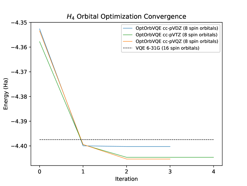
Figure 1: Convergence of OptOrbVQE as a function of the outer loop iteration number for H4 at the near-equilibrium H-H distance of 1.23 Å.

We set the number of spin orbitals to be 8 for H4, the number of spin orbitals for this system in the minimal STO-3G basis set. Fig. 1 illustrates the convergence of the OptOrbVQE algorithm as a function of the outer loop iteration number for various starting basis sets. We compare the results to that obtained from VQE in the 6-31G basis using 2-UCCSD as the ansatz. Under these conditions, VQE is using 16 qubits. Despite the fact that OptOrbVQE is using half the number of qubits as VQE, we find that it achieves a lower ground state energy for all the starting basis sets used. This lower energy is achieved after just the $n=1$ outer loop iteration, which corresponds to carrying out the orbital rotation subroutine once and the VQE subroutine twice. The energy is lowered further when cc-pVTZ and cc-pVQZ are used as starting basis sets with further iterations.

4.1.2 LiH

For LiH, we use 1-UCCSD as the ansatz. We set the number of spin orbitals for OptOrbVQE to be 12, the number of spin orbitals for this system in the minimal STO-3G basis set. We compute the ground state energy at the near-equilibrium Li-H distance of 1.595 Å as well as the binding curve of LiH.

Figure 2: Convergence of OptOrbVQE as a function of the outer loop iteration number for LiH at the near-equilibrium bond distance of 1.595 Å.

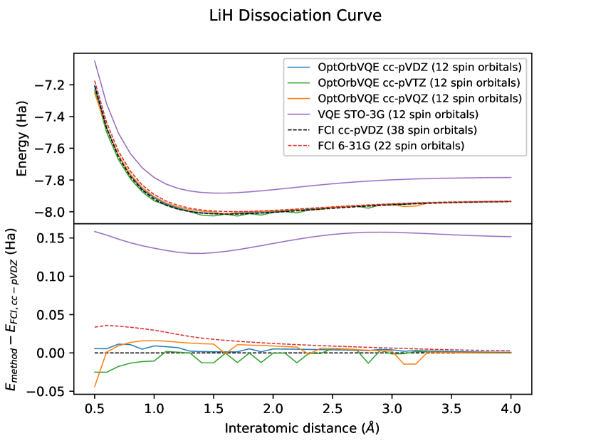
Figure 3: Top: Dissociation curve of LiH. Bottom: Difference of energy relative to FCI (cc-pVDZ).

Fig. 2 illustrates the convergence of OptOrbVQE as a function of the outer loop iteration number. We find that OptOrbVQE achieves a lower energy than VQE in the 6-31G basis after the $n=1$ iteration. The energy is further improved with additional iterations. In particular, OptOrbVQE using cc-pVTZ as the starting basis surpasses the FCI energy in the cc-pVDZ basis at the $n=7$ iteration. OptOrbVQE starting from the cc-pVDZ basis also approaches, but does not surpass this value. We also note that starting from a larger basis does not always result in a more accurate value, as can be seen from OptOrbVQE (cc-pVQZ starting basis) not achieving the same accuracy as the other two starting basis sets.

Fig. 3 illustrates the results obtained for the binding curve of LiH. We can see that OptOrbVQE easily outperforms VQE using the same number of qubits. OptOrbVQE consistently achieves an energy lower than the FCI energy in the 6-31G basis. OptOrbVQE also often achieves an energy lower than the FCI energy in the cc-pVDZ basis, although this is not guaranteed and sometimes fails to do so.

4.1.3 BeH2

In this section we test OptOrbVQE on BeH2, a linear molecule with a near-equilibrium Be-H bond distance of 1.3264 Å. 1-UCCSD is the ansatz used. The number of spin orbitals used by OptOrbVQE is set to 14, the number of spin orbitals for this system in the minimal STO-3G basis.

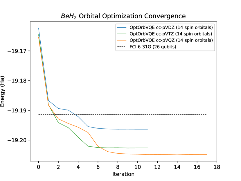
Figure 4: Convergence of OptOrbVQE as a function of the outer loop iteration number for BeH2 at the near-equilibrium Be-H bond distance of 1.3264 Å.

Fig. 4 illustrates the convergence of OptOrbVQE at the equilibrium configuration. We find that starting from either the cc-pVTZ or cc-pVQZ basis set results in OptOrbVQE surpassing the FCI energy in the 6-31G basis at the $n=2$ iteration. Further iterations result in improved energy. Starting from the cc-pVDZ also surpasses the FCI (6-31G basis), but requires more iterations to do so.

4.1.4 H2O

In this section we test OptOrbVQE on the H2O molecule. The ansatz used is 1-UCCSD. The number of spin orbitals used by OptOrbVQE is set to 14, the number of spin orbitals for this molecule in the minimal STO-3G basis. Fig. 5 plots the difference of the OptOrbVQE energy from the FCI energy in the 6-31G basis for H2O at the near-equilibrium configuration of O-H distance 0.9578 Å and H-O-H bond angle of 104.4778 degrees. These results are different from the other systems presented in that while the method still easily outperforms VQE using the same number of spin orbitals, we do not observe OptOrbVQE using a minimal number of spin orbitals to surpass the FCI energy in the larger 6-31G basis. OptOrbVQE can however be observed to approach the FCI (6-31G basis) energy at the milli-hartree level, with the energy difference converging to approximately $2.5\times 10^{-3}$ Hartree when using cc-pVQZ as the starting basis. One notable feature about this convergence curve is that the rate of convergence is most rapid up until the $n=3$ iteration, then hits a plateau. The energy then fluctuates until the maximum number of iterations is reached, indicating the possible presence of multiple local minima which differ in energy at the milli-Hartree level. A similar trend is observed when starting from the cc-pVTZ basis, although the converged energy accuracy is worse and the fluctuations are less pronounced in this case. It is also worth noting that the $0th$ iteration of OptOrbVQE outperforms VQE in Fig. 5. Because the initial partial unitary for OptOrbVQE is set to be the matrix which selects the $N$ lowest energy spin orbitals, the $0th$ iteration corresponds to starting with a large basis, but reducing the active space to one the same size as the STO-3G basis. Thus, using orbital optimization is often not necessary to outperform VQE in the STO-3G basis. The main benefit of orbital optimization is further accuracy improvements at the milli-Hartree level.

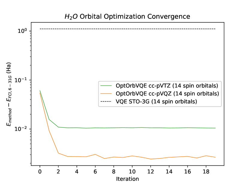
Figure 5: Convergence of OptOrbVQE as a function of the outer loop iteration number for H2O at the near-equilibrium O-H bond distance of 0.9578 Å and bond angle 104.4776 degrees.

4.2 Increasing Qubit Resources

One important feature of OptOrbVQE is that the number of spin orbitals used is a tunable parameter that can be set to any positive integer up to the number used by the starting basis set. The previous sections examined the performance of OptOrbVQE for various systems when using a number of spin orbitals equal to the minimal STO-3G basis. In this section we increase the number of spin orbitals used by OptOrbVQE in order to examine the potential for the method to further improve energy accuracies as the capabilities of quantum computers improve with time. We test OptOrbVQE on H2 using even integer numbers of spin orbitals from 4 to 16. Qiskit’s AerSimulator and AerPauliExpectation are used to obtain ideal noiseless results as in §4.1. The optimizer used is L-BFGS-B and the ansatz used is 1-UCCSD. Fig. 6 plots the difference of the OptOrbVQE energy at the near-equilibrium bond distance of 0.735 Å using OptOrbVQE and the FCI energy in the cc-pVTZ basis (56 spin orbitals). The FCI energy in the cc-pVDZ basis (20 spin orbitals) is also included for reference. The most significant (but expected) feature of this plot is that the energy accuracy obtained by OptOrbVQE can be improved by increasing the number of spin orbitals that it uses. This comes with the caveat that using more qubits does not always result in a lower converged energy. Several plateaus can be seen over the interval considered. For example, increasing the number of spin orbitals from 6 to 8 does not result in significantly improved energy when starting from either the cc-pVTZ or cc-pV5Z basis sets. Increasing the number of qubits from 10 to 16 also does not appear to result in improved energies when starting from the cc-pVQZ basis. Another notable feature of this plot is that for a given number of qubits, starting from a larger basis set does not always result in lower energy. This can be seen from OptOrbVQE starting from the cc-pVQZ basis achieves a lower energy than starting from the cc-pV5Z basis for 8 and 10 qubits. Finally, we note that in Fig. 6, the green curve compares the logarithmic difference between the energy obtained by OptOrbVQE starting from the cc-pVTZ basis and the FCI energy in the full 56 spin-orbital cc-pVTZ basis. The highest degree of accuracy obtained at 16 spin-orbitals is approximately 3 milliHartree. There are several factors contributing to this discrepancy: 1. OptOrbVQE consists of two optimization subproblems, neither of which is guaranteed to converge to the global minimum. Each may converge to a spurious local minima or within a neighborhood of the global minimum. 2. The VQE subproblem utilizes a wavefunction ansatz. This comes with an associated ansatz representation error that is not present in the classical FCI algorithm. 3. It is well-known that large basis set expansions improve the ability of computational methods to capture energy contributions that arise from electron correlation effects, in particular dynamic correlation. Although orbital optimization helps the method capture some of this energy contribution, its smaller basis size precludes it from capturing all of it.

The first two points listed here may also help to explain some un-intuitive behavior exhibited by some of the tests in this paper. For example, in Fig. 2, the largest starting basis used by OptOrbVQE, cc-pVQZ, is the one which achieved the least accurate energy among the three starting basis sets considered. This is counter to what one would intuitively expect, where the more flexible variational space should give it the potential to achieve the highest quality accuracy. Furthermore, several plateaus are observed for all three starting basis sets. Similarly, in Fig. 6 there are several instances where increasing the size of the variational space through an increase in the number of qubits does not strictly result in an increase in accuracy, but rather appears to occasionally result in a plateau. There are a few possible explanations for this behavior. We note that in order for the benefits of an increased variational space to be apparent in the final accuracy obtained, it is necessary for both the orbital optimization and VQE subproblems to converge sufficiently close to their global minima and for the VQE ansatz to have sufficient representation accuracy in the rotated basis sets determined by the orbital optimization subroutine at each iteration. If any of these conditions are not met, the final energy accuracy may not reach its full potential. We defer a more in-depth study on how to improve the convergence of OptOrbVQE to future work. For example, one could investigate incorporating adaptive ansatz strategies ^{26, 27} into the VQE subproblem. The intuition behind this approach is that an adaptive ansatz may be better suited for representing the ground state of a system than a fixed ansatz when the basis set representation itself is iteratively changing. A second possibility would be to add a random perturbation to the initial parameters of each VQE iteration. In these tests, a random perturbation is added to the initial partial unitary to help the orbital optimization escape from shallow local minima, but the VQE subproblem may also benefit from a similar initialization.

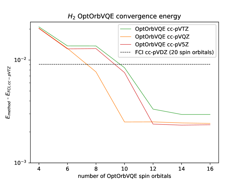
Figure 6: Converged energy of OptOrbVQE as a function of the number of spin orbitals for H2 at the near-equilibrium bond distance of 0.735 Å.

4.3 Robustness to Noise

We now investigate the robustness of the OptOrbVQE algorithm to noise, which we carry out in two stages using the binding curve of the H2 molecule as a test system. In §4.3.1 we incorporate statistical sampling as the only source of the noise. On quantum hardware, this type of noise arises from the repeated circuit preparation and observable measurement process. For example, to measure the quantity $\bra{\psi_{\text{ref}}}\hat{U}^{\dagger}(\boldsymbol{\theta})\hat{H}\hat{U}(\boldsymbol{\theta})\ket{\psi_{\text{ref}}}$ we would prepare the circuit $\hat{U}(\boldsymbol{\theta})$ $n$ times, measuring each of the Pauli terms $\hat{P}_{i}$ in Eq. (4) $n$ times and classically compute the weighted sum of their expectation values. Because this form of noise is independent of the ansatz circuit depth, starting with this form of noise allows us to compare OptOrbVQE using a smaller basis to VQE using a larger basis while keeping the effects that would arise from the difference in circuit depth between these two problem instances separate. In §4.3.2 we add a local depolarizing noise model to the statistical noise.

4.3.1 Statistical Sampling Noise

For the noisy simulations, we choose COBYLA as the classical optimizer. Its lack of a need to calculate gradient information makes it more resilient to noise than L-BFGS-B. The ansatz used is 1-UCCSD. The mapping used is Jordan-Wigner. $10^{6}$ circuit samples are used for observable measurements. OptOrbVQE is set to use cc-pVQZ as the starting basis and uses 4 spin orbitals in the transformed basis. We compare it to VQE in the 6-31G basis (8 spin orbitals), using the FCI (6-31G basis) as a baseline. Fig. 7 illustrates the results obtained for these tests. The outer loop stopping tolerance is set to $10^{-3}$. The error bars are calculated internally by Qiskit, which records the statistical variance $\sigma$ associated with expectation values from $n$ circuit samples and returns the error as $\sqrt{\frac{\sigma}{n}}$.

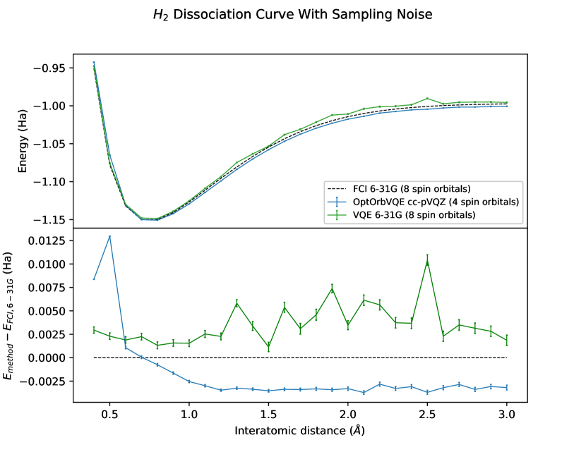
Figure 7: Top: binding curve of H2 using $10^{6}$ circuit samples. Bottom: difference in energy from the FCI (6-31G basis) energy.

We can see that in the presence of statistical sampling noise, OptOrbVQE retains its ability to achieve a lower ground state energy than VQE while only using half the number of qubits for interatomic distances 0.6 Å and greater.

4.3.2 Depolarizing Noise

In order to model the effects of gate noise, we add a local depolarizing channel to each one-qubit gate and a tensor product of two local depolarizing channels to each two-qubit gate. This has the effect that every time a one-qubit gate is applied, one of the three Pauli operators (with equal likelihood) is also applied with probability $p_{error}$. For two-qubit gates, this probabilistic error event occurs independently for each qubit involved. In this work we set $p_{error}=10^{-3}$. No error mitigation techniques are used. Aside from adding gate noise, the methodology remains the same as in §4.3.1, except that the ansatz is changed from 1-UCCSD to a hardware-efficient ansatz shown in Fig. 8.

@C=0.3em @R=.3em & X R_y(θ_0) 1 R_y(θ_4) 1 R_y(θ_8)
R_y(θ_1) 1 R_y(θ_5) 1 R_y(θ_9)
X R_y(θ_2) 1 R_y(θ_6) 1 R_y(θ_10)
R_y(θ_3) R_y(θ_7) R_y(θ_11)

Figure 8: Ansatz used for H2 simulations with depolarizing noise.

In Qiskit, this corresponds to the Real Amplitudes circuit with the number of repetitions set to 2. The first layer of this circuit prepares the qubits in the Hartree Fock state. The parameters are initialized to zero. We compare OptOrbVQE to VQE (STO-3G basis), using the FCI (6-31G basis) energy as a baseline. The results of these tests are shown in Fig. 9.

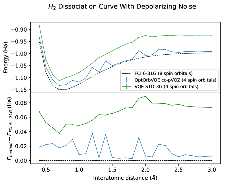
Figure 9: Top: binding curve of H2 using $10^{6}$ circuit samples with $p_{error}=10^{-3}$. Bottom: difference in energy from the FCI (6-31G basis) energy.

We find that OptOrbVQE consistently achieves lower energy than VQE when using the same number of qubits. Unlike in §4.3.1 when only statistical sampling noise was used, OptOrbVQE no longer achieves energy lower than FCI in the 6-31G basis. It does, however, approach this reference energy at the milli-Hartree level for several interatomic distances.

5 Discussion and Conclusions

One of the main challenges that exists today in quantum computing is demonstrating quantum advantage on a problem with practical utility. One such problem is calculating the ground state of electronic chemical systems to high accuracy when compared to laboratory results. In this work we have demonstrated that OptOrbVQE offers a clear path towards this goal in two ways: 1. When using a number of qubits equal to that in a minimal basis, OptOrbVQE consistently achieves higher accuracy than VQE using a minimal basis set. In many cases it can even outperform VQE methods of larger basis sets using a fraction of the number of qubits. As an aside, we also note that because these numerical demonstrations used an initial partial unitary which selects the subset of spin-orbitals with the lowest Hartree-Fock energy, the 0th OptOrbVQE energy is equivalent to that which would be obtained by VQE using an active space selected in this manner. Thus, we observe that OptOrbVQE achieves more accurate results than VQE when the starting underlying full orbital space basis is the same as well. 2. The number of qubits used by OptOrbVQE is a tunable parameter. Increasing the number of qubits typically has the effect of improving the energy accuracy, which provides a convenient method for systematically demonstrating improved results as the capabilities of quantum computers progress.

This improved performance comes at the cost of running the orbital optimization and VQE subproblems multiple times. While we find that our classical simulations can in some instances utilize 10 or more iterations before the stopping condition is reached, the bulk of the convergence typically occurs during the first 2-5 iterations. These first few iterations are typically sufficient for the method to surpass VQE and FCI methods of larger basis sets. A user of this algorithm could simply choose to limit the number of iterations to 2-5 and still see most of the benefit of this method over using VQE with a basis set of the same size or larger.

One final point to note is that although we have used VQE to demonstrate this method, many other quantum eigensolvers could be used in its place to achieve different goals or to improve the performance. The main criterion is that the eigensolver returns an improved estimate for the eigenstate(s) over its input state(s). For example, Quantum Phase Estimation (QPE) ²⁸ would not be a suitable choice of eigensolver because it returns an estimate of the eigenvalue but does not return an improved estimate of the eigenstate itself. However, an algorithm such as $\alpha$-VQE ²⁹ that uses QPE as a subroutine could be a suitable eigensolver because it iteratively improves the estimation of the ground state. Other suitable ground state eigensolvers that could be explored in this orbital optimization framework include Quantum Imaginary Time Evolution (QITE) ¹⁶, variational QITE ¹⁷, Quantum Monte Carlo ¹⁸, ADAPT-VQE ²⁶, and qubit-ADAPT-VQE ²⁷. Excited state eigensolvers could be explored as well. The three most obvious candidates would be Quantum Subspace Expansion (QSE) ³⁰, quantum Equation of Motion (qEoM) ³, and EOM-VQE ³¹. These methods operate by first performing the ground state search using an algorithm such as VQE, then performing a classical post-processing diagonalization step to find low-lying excited states of the Hamiltonian. Thus, OptOrbVQE could be used as a ground state solver for these methods. Two other excited states eigensolver for which it would be straightforward to incorporate this orbital optimization procedure would be multistate contracted VQE (MC-VQE) ³² and Subspace Search VQE (SSVQE) ³³. These two methods both apply an ansatz circuit to a set of mutually orthogonal input states and minimize an objective function consisting of a weighted sum of expectation values of the Hamiltonian with respect to each of the resulting parameterized states. OptOrbVQE could easily be generalized to “OptOrbMC-VQE” or “OptOrbSSVQE” by modifying Eq. (9) to be a weighted sum of the transformed Hamiltonian with respect to mutually orthogonal parameterized states in the same manner as these methods. Orbital optimization could also be applied to the quantum Orbital Minimization Method (qOMM) ³⁴ by modifying Eq. (9) in an analogous way. These methods all find low-lying excited states simultaneously through the minimization of a single objective function. Variational Quantum Deflation (VQD) ³⁵ is different from these other methods in that it finds the low-lying excited states sequentially through a series of minimization procedures. Thus, the application of orbital optimization to VQD would be more involved than simply modifying Eq. (9), but could still be investigated. We leave the investigation of the application of the orbital optimization procedure to these eigensolvers to future work.

The work is supported in part by the US National Science Foundation under award CHE-2037263 and by the US Department of Energy via grant DE-SC0019449. YL is supported in part by the National Natural Science Foundation of China 12271109.

References

- Helgaker et al. 2014 Helgaker, T.; Jorgensen, P.; Olsen, J. Molecular Electronic-Structure Theory; Wiley, 2014
- McCaskey et al. 2019 McCaskey, A. J.; Parks, Z. P.; Jakowski, J.; Moore, S. V. et al. Quantum chemistry as a benchmark for near-term quantum computers. npj Quantum Information 2019, 5, 99
- Ollitrault et al. 2020 Ollitrault, P. J.; Kandala, A.; Chen, C.-F.; Barkoutsos, P. K. et al. Quantum equation of motion for computing molecular excitation energies on a noisy quantum processor. Phys. Rev. Research 2020, 2, 043140
- Kandala et al. 2017 Kandala, A.; Mezzacapo, A.; Temme, K.; Takita, M. et al. Hardware-efficient variational quantum eigensolver for small molecules and quantum magnets. Nature 2017, 549, 242–246
- Metcalf et al. 2020 Metcalf, M.; Bauman, N. P.; Kowalski, K.; de Jong, W. A. Resource-Efficient Chemistry on Quantum Computers with the Variational Quantum Eigensolver and the Double Unitary Coupled-Cluster Approach. Journal of Chemical Theory and Computation 2020, 16, 6165–6175, doi: 10.1021/acs.jctc.0c00421
- Huang et al. 2022 Huang, R.; Li, C.; Evangelista, F. A. Leveraging small scale quantum computers with unitarily downfolded Hamiltonians. 2022,
- Claudino et al. 2021 Claudino, D.; Peng, B.; Bauman, N. P.; Kowalski, K. et al. Improving the accuracy and efficiency of quantum connected moments expansions*. Quantum Science and Technology 2021, 6, 034012
- Motta et al. 2020 Motta, M.; Gujarati, T. P.; Rice, J. E.; Kumar, A. et al. Quantum simulation of electronic structure with a transcorrelated Hamiltonian: improved accuracy with a smaller footprint on the quantum computer. Phys. Chem. Chem. Phys. 2020, 22, 24270–24281
- Sokolov et al. 2022 Sokolov, I. O.; Dobrautz, W.; Luo, H.; Alavi, A. et al. Orders of magnitude reduction in the computational overhead for quantum many-body problems on quantum computers via an exact transcorrelated method. 2022,
- Mizukami et al. 2020 Mizukami, W.; Mitarai, K.; Nakagawa, Y. O.; Yamamoto, T. et al. Orbital optimized unitary coupled cluster theory for quantum computer. Phys. Rev. Research 2020, 2, 033421
- Yalouz et al. 2021 Yalouz, S.; Senjean, B.; Günther, J.; Buda, F. et al. A state-averaged orbital-optimized hybrid quantum–classical algorithm for a democratic description of ground and excited states. Quantum Science and Technology 2021, 6, 024004
- Tilly et al. 2021 Tilly, J.; Sriluckshmy, P. V.; Patel, A.; Fontana, E. et al. Reduced density matrix sampling: Self-consistent embedding and multiscale electronic structure on current generation quantum computers. Phys. Rev. Research 2021, 3, 033230
- Takeshita et al. 2020 Takeshita, T.; Rubin, N. C.; Jiang, Z.; Lee, E. et al. Increasing the Representation Accuracy of Quantum Simulations of Chemistry without Extra Quantum Resources. Phys. Rev. X 2020, 10, 011004
- Li and Lu 2020 Li, Y.; Lu, J. Optimal Orbital Selection for Full Configuration Interaction (OptOrbFCI): Pursuing the Basis Set Limit under a Budget. Journal of Chemical Theory and Computation 2020, 16, 6207–6221, PMID: 32786901
- Peruzzo et al. 2014 Peruzzo, A.; McClean, J.; Shadbolt, P.; Yung, M.-H. et al. A variational eigenvalue solver on a photonic quantum processor. Nature Communications 2014, 5, 4213
- Motta et al. 2020 Motta, M.; Sun, C.; Tan, A. T. K.; O’Rourke, M. J. et al. Determining eigenstates and thermal states on a quantum computer using quantum imaginary time evolution. Nature Physics 2020, 16, 205–210
- McArdle et al. 2019 McArdle, S.; Jones, T.; Endo, S.; Li, Y. et al. Variational ansatz-based quantum simulation of imaginary time evolution. npj Quantum Information 2019, 5, 75
- Huggins et al. 2022 Huggins, W. J.; O’Gorman, B. A.; Rubin, N. C.; Reichman, D. R. et al. Unbiasing fermionic quantum Monte Carlo with a quantum computer. Nature 2022, 603, 416–420
- McArdle et al. 2020 McArdle, S.; Endo, S.; Aspuru-Guzik, A.; Benjamin, S. C. et al. Quantum computational chemistry. Rev. Mod. Phys. 2020, 92, 015003
- Anis et al. 2021 Anis, M. S.; Abraham, H.; AduOffei; Agarwal, R. et al. Qiskit: An Open-source Framework for Quantum Computing. 2021
- Paszke et al. 2019 Paszke, A.; Gross, S.; Massa, F.; Lerer, A. et al. In Advances in Neural Information Processing Systems 32; Wallach, H., Larochelle, H., Beygelzimer, A., d'Alché-Buc, F. et al. , Eds.; Curran Associates, Inc., 2019; pp 8024–8035
- Gao et al. 2018 Gao, B.; Liu, X.; Chen, X.; Yuan, Y.-x. A New First-Order Algorithmic Framework for Optimization Problems with Orthogonality Constraints. SIAM Journal on Optimization 2018, 28, 302–332
- Byrd et al. 1995 Byrd, R. H.; Lu, P.; Nocedal, J.; Zhu, C. A Limited Memory Algorithm for Bound Constrained Optimization. SIAM Journal on Scientific Computing 1995, 16, 1190–1208
- Romero et al. 2018 Romero, J.; Babbush, R.; McClean, J. R.; Hempel, C. et al. Strategies for quantum computing molecular energies using the unitary coupled cluster ansatz. Quantum Science and Technology 2018, 4, 014008
- Sun et al. 2018 Sun, Q.; Berkelbach, T. C.; Blunt, N. S.; Booth, G. H. et al. PySCF: the python-based simulations of chemistry framework. Wiley Interdisciplinary Reviews: Computational Molecular Science 2018, 8, e1340
- Grimsley et al. 2019 Grimsley, H. R.; Economou, S. E.; Barnes, E.; Mayhall, N. J. An adaptive variational algorithm for exact molecular simulations on a quantum computer. Nature Communications 2019, 10, 3007
- Tang et al. 2021 Tang, H. L.; Shkolnikov, V.; Barron, G. S.; Grimsley, H. R. et al. Qubit-ADAPT-VQE: An Adaptive Algorithm for Constructing Hardware-Efficient Ansätze on a Quantum Processor. PRX Quantum 2021, 2, 020310
- Aspuru-Guzik et al. 2005 Aspuru-Guzik, A.; Dutoi, A. D.; Love, P. J.; Head-Gordon, M. Simulated Quantum Computation of Molecular Energies. Science 2005, 309, 1704–1707
- Wang et al. 2019 Wang, D.; Higgott, O.; Brierley, S. Accelerated Variational Quantum Eigensolver. Phys. Rev. Lett. 2019, 122, 140504
- McClean et al. 2017 McClean, J. R.; Kimchi-Schwartz, M. E.; Carter, J.; de Jong, W. A. Hybrid quantum-classical hierarchy for mitigation of decoherence and determination of excited states. Phys. Rev. A 2017, 95, 042308
- Asthana et al. 2022 Asthana, A.; Kumar, A.; Abraham, V.; Grimsley, H. et al. Equation-of-motion variational quantum eigensolver method for computing molecular excitation energies, ionization potentials, and electron affinities. 2022,
- Parrish et al. 2019 Parrish, R. M.; Hohenstein, E. G.; McMahon, P. L.; Martínez, T. J. Quantum Computation of Electronic Transitions Using a Variational Quantum Eigensolver. Phys. Rev. Lett. 2019, 122, 230401
- Nakanishi et al. 2019 Nakanishi, K. M.; Mitarai, K.; Fujii, K. Subspace-search variational quantum eigensolver for excited states. Phys. Rev. Research 2019, 1, 033062
- Bierman et al. 2022 Bierman, J.; Li, Y.; Lu, J. Quantum Orbital Minimization Method for Excited States Calculation on a Quantum Computer. Journal of Chemical Theory and Computation 2022, 18, 4674–4689, PMID: 35876650
- Higgott et al. 2019 Higgott, O.; Wang, D.; Brierley, S. Variational Quantum Computation of Excited States. Quantum 2019, 3, 156