FAKD: Feature Augmented Knowledge Distillation for Semantic Segmentation

Abstract

In this work, we explore data augmentations for knowledge distillation on semantic segmentation. To avoid over-fitting to the noise in the teacher network, a large number of training examples is essential for knowledge distillation. Image-level argumentation techniques like flipping, translation or rotation are widely used in previous knowledge distillation framework. Inspired by the recent progress on semantic directions on feature-space, we propose to include augmentations in feature space for efficient distillation. Specifically, given a semantic direction, an infinite number of augmentations can be obtained for the student in the feature space. Furthermore, the analysis shows that those augmentations can be optimized simultaneously by minimizing an upper bound for the losses defined by augmentations. Based on the observation, a new algorithm is developed for knowledge distillation in semantic segmentation. Extensive experiments on four semantic segmentation benchmarks demonstrate that the proposed method can boost the performance of current knowledge distillation methods without any significant overhead. Code is available at: https://github.com/jianlong-yuan/FAKD.

Introduction

Semantic segmentation/Pixel labeling is a fundamental problem in computer vision, which is widely used in scene parsing, human body parsing, and many downstream applications. It is a per-pixel classification problem that assigns each pixel in an image to a specific set of predefined classes. With the development of deep learning, semantic segmentation has made tremendous progress in recent years and achieved impressive results on large benchmark datasets (Everingham et al. 2010; Mottaghi et al. 2014; Cordts et al. 2016; Zhou et al. 2017). However, advanced segmentation models usually require complicated model designs and expensive computations. As a result, it limits the potential for computationally constrained applications on devices.

To alleviate the computational cost, some efforts have been devoted to designing lightweight networks, especially for semantic segmentation (Yu et al. 2018a; Mehta et al. 2018; Zhao et al. 2018a; Yu et al. 2021; Chen et al. 2019; Li et al. 2019). In addition, knowledge distillation (KD) attracts attention to train lightweight semantic segmentation networks effectively by leveraging the knowledge from the teacher network. The conventional KD method for the classification problem is to apply a Kullback–Leibler (KL) divergence between the output of the teacher and the student network for each example. However, mimicking every pixel’s class distribution is inappropriate for semantic segmentation since the noise accumulated from the pixel-level activation may degenerate the performance. SKDS (Liu et al. 2019, 2020) aggregates a sub-set of different spatial locations according pair-wise relations. Moreover, IFVD (Hou et al. 2020) exploits the inter-class relations among different locations. CWD (Shu et al. 2021) proposes channel-wise knowledge distillation by minimizing the channel distribution, indicating the spatial location for each class. CIRKD (Yang et al. 2022) focuses on transferring structured pixel-to-pixel and pixel-to-region relations among the whole images.

However, the teacher and student can have different training procedures, which makes the transfer challenging even with the sophisticated objective function for semantic segmentation. Moreover, optimization based on a limited number of training examples can make the knowledge transfer for the whole data distribution more challenging. To capture the data distribution on unseen data, augmentation is a prevalent strategy to improve the generalization of deep models. Concretely, image-level data augmentation operators, including random crop, random scale, and flip (He et al. 2016), are widely applied in existing methods. Apparently, the number of applicable augmentation operators for each image is limited, which may be insufficient for knowledge distillation that has to mimic the diverse patterns from the teacher. Moreover, this kind of image space based augmentations has to be fed forward from the input to the whole network, thus only a limited number of augmentations can be adopted for optimization.

Recently, some works (Upchurch et al. 2017; Li, Zuo, and Zhang 2016; Bengio et al. 2013; Wang et al. 2019, 2021a) propose there are many semantic directions in the deep feature space, such that translating a data sample along one of these directions in the feature space produces a feature representation corresponding to another sample with the same class but different semantics. Meanwhile, compared to the augmentation in raw images, that in high-level features is more flexible and can be obtained along with arbitrary semantic directions. Therefore, motivated by these, we propose to augment the samples in the feature space to apply sufficient and diverse augmentations for knowledge distillation.

Specifically, the direction of intra-class variation that contains the semantic information of each class is essential and adopted for the perturbation in feature space. Based on the intra-class variance, we augment examples in feature space according to the corresponding Gaussian distribution. Thanks to this procedure, we can have an infinite number of augmentations from feature space, and an upper bound of the loss function can be optimized accordingly to transfer the knowledge from the teacher sufficiently. With massive augmented examples for the student, the nice properties, e.g., large margin, from the teacher can be preserved for generalization.

Finally, based on the distribution definition, different knowledge distillation objective functions will have different surrogate functions for the upper bounds of infinite augmentations. In this work, two types of Kullback–Leibler divergence-based knowledge distillation loss are investigated, and the corresponding loss functions are derived. Experiment results show that the proposed feature augmentation method can improve the performance over baseline KL–based knowledge distillation losses on four different datasets.

Concretely, our contributions are three-fold:

• We propose a novel feature augmented knowledge distillation (FAKD) method for semantic segmentation. Specifically, the student model will mimic the teacher model with infinite augmented samples. To the best of our knowledge, it is the first time that the feature-level augmentation method has been explored in knowledge distillation for semantic segmentation.

• We provide a theoretical analysis from the infinite number of augmentations in feature space to the upper-bound loss, so as to theoretically demonstrate our proposal for different knowledge distillation methods.

• We demonstrate the effectiveness of our approach applying various network structures on four benchmark datasets: ADE20K, Pascal Context, Cityscapes, and Pascal VOC.

Related Work

Semantic Segmentation

Semantic segmentation can be regarded as a pixel-level classification problem. The fully convolutional network(FCN) (Long, Shelhamer, and Darrell 2015) is a pioneering work in the field of semantic segmentation, which can adapt to any scale input. To improve the performance of the segmentation network, many researchers try to improve FCN in different ways. In (Chen et al. 2017; Yu and Koltun 2015; Zhao et al. 2017; Yang et al. 2018; Peng et al. 2017; Chen et al. 2018; Yuan et al. 2020a), the receptive field is enlarged to capture more details. In (Zhang et al. 2018; He et al. 2019; Lin et al. 2017; Zhou et al. 2019; Yuan, Chen, and Wang 2020; Yuan et al. 2018; Yu et al. 2020), the contextual information is combined to improve the semantic understanding of the model. In (Ding et al. 2019; Bertasius, Shi, and Torresani 2016; Yuan et al. 2020b; Zhen et al. 2020; Takikawa et al. 2019; Yu et al. 2018b; Chen et al. 2016), the boundary information is considered to boost the segmentation accuracy further. In (Wang et al. 2018; Fu et al. 2019; Zhong et al. 2020; Huang et al. 2019; Zhao et al. 2018b), some new attention modules are designed to enrich the representations of the feature map. Moreover, (Xie et al. 2021; Zheng et al. 2021; Wang et al. 2021b) introduce transformer blocks into the Semantic Segmentation task, which boosts the performance with a large margin. Although the state-of-the-art performance keeps improving nowadays, the models have become larger than before. The high computational cost limits the application of the segmentation models over resource-limited mobile devices.

Efficient segmentation networks attract wide attention due to the need for real-time inference. Most of the works pay attention to designing lightweight networks with cheap operations. ENet (Paszke et al. 2016) is a efficient segmentation network with early downsampling, lightweight decoder. ESPNet (Mehta et al. 2018) introduces more cheap spatial pyramid of dilated convolution. ICNet (Zhao et al. 2018a) proposes a cascade structure to use low-resolution and high-resolution features. BiSeNet (Yu et al. 2018a) combines a spatial path and a context path to process features efficiently.

Knowledge distillation

Knowledge distillation has been extensively studied in recent years. The core idea of knowledge distillation is to transfer meaningful knowledge from a cumbersome teacher into a smaller and faster student. Most knowledge distillation methods for image classification networks could be classified into three classes, probability-based, feature-based and relation-based methods. (Hinton, Vinyals, and Dean 2015; Zhou et al. 2021) distill the output logits of the teacher network as soft labels to the student. Feature-based knowledge distillation methods (Romero et al. 2014; Heo et al. 2019; Zagoruyko and Komodakis 2016) focuses on the feature maps. Finally, relation-based KD (Peng et al. 2019; Park et al. 2019; Qian, Li, and Hu 2022) aligns correlations among multiple instances between the student and teacher networks. However, these image-level KD methods are not suitable for pixel-level semantic segmentation.

Some works pay attention to utilizing knowledge distillation to semantic segmentation. The pioneering work (Liu et al. 2019, 2020) proposes Structured Knowledge Distillation (SKDS), which enables the output of the student model to transfer the structure knowledge among pixels from the teacher model to the student model through pairwise relationships and adversarial training. (Wang et al. 2020) focuses on intra-class feature variations between pixels with the same label, where the set of cosine distances between the features of each pixel and its corresponding class prototype is constructed to convey structural knowledge. (Shu et al. 2021) proposes channel-wise distillation to guide the student to mimic the teacher’s channel-wise distribution, which indicates the spatial location for each class. (Yang et al. 2022) focuses on transferring structured pixel-to-pixel and pixel-to-region relations among the whole images. These methods try to develop objective functions to align useful knowledge between the teacher and the student network. Our approach, however, is to face how effective knowledge distillation can be performed when teacher and student training procedures are not aligned in real-life scenarios.

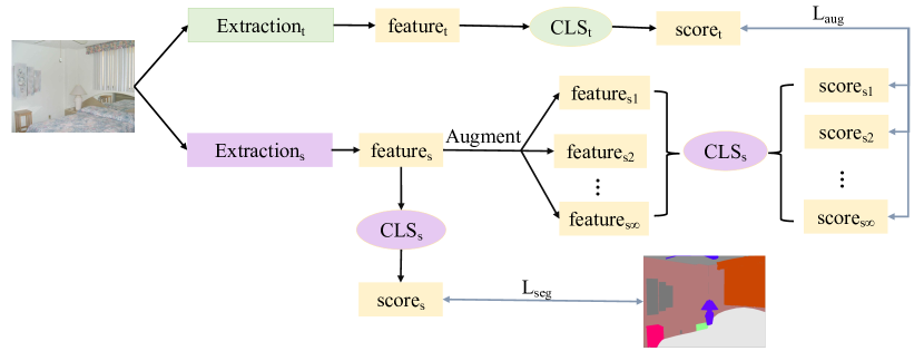
Figure 1: Illustration of the proposed feature augmented knowledge distillation (FAKD). The parameters of the teacher network are fixed during training. The feature of the student network is augmented to mimic the effect of infinite samples. The weight for the ‘CLS_s’ is shared.

Methods

The overall pipeline of the proposed method, feature augmented knowledge distillation (FAKD), is illustrated in Figure 1. We will first revisit two Kullback–Leibler (KL) divergence-based knowledge distillation losses and then investigate the new loss functions with an infinite number of augmentations.

Revisit Knowledge Distillation

KL divergence is a standard metric to evaluate the difference between distributions, which is also widely used in designing knowledge distillation objective functions. In this subsection, we will revisit two popular knowledge distillation objective functions, i.e., pixel-wise distillation (Hinton, Vinyals, and Dean 2015) and channel-wise distillation (Shu et al. 2021).

The pixel-wise distillation (PD) is straightforward that mimics the output from the teacher for each pixel. It directly extends the knowledge distillation protocol for classification to semantic segmentation and is widely used as a baseline method in existing semantic segmentation distillation works (Liu et al. 2019; Hou et al. 2020). The channel-wise distillation (CWD) (Shu et al. 2021) aligns the output distribution for each channel rather than the pixel. It achieves state-of-the-art performance on benchmark semantic segmentation datasets.

Let $s_{i}\in\mathbb{R}^{A}$ and $t_{i}\in\mathbb{R}^{A}$ be the feature of the student and teacher of the $i$ pixel. $A$ is the number of the feature channel before the final classifier. A linear classifier is usually applied to the feature to get the final logit, for example for the teacher’s output of the pixel $i$ for the $c$ class, $q^{c}_{t_{i}}=\omega_{c}^{\top}t_{i}+b_{c}$. The loss function for the pixel-wise distillation (Hinton, Vinyals, and Dean 2015; Liu et al. 2019, 2020) can be written as

$$\ell_{PD}=\frac{1}{M}\sum_{i=1}^{M}\sum_{c=1}^{C}\\ \left(-\frac{e^{\omega_{c}^{\top}t_{i}+b_{c}}}{{\sum_{k=1}^{C}e^{{\omega_{k}^{\top}t_{k}+b_{k}}}}}\log\left(\frac{e^{\omega_{c}^{\top}s_{i}+b_{c}}}{{\sum_{k=1}^{C}e^{{\omega_{k}^{\top}s_{k}+b_{k}}}}}\right)\right),$$ (1)

where $M$ donates the number of pixels and $C$ is the number of categories. $W=[\omega_{1},\dots,\omega_{C}]^{\top}\in\mathbb{R}^{C\times A}$ and $B=[b_{1},\dots,b_{C}]^{\top}\in\mathbb{R}^{C}$ are the classification convolution weights and bias, respectively. The softmax operator is applied to every pixel prediction for all classes to find out the class distribution for all pixels. Then the KL divergence between two class distributions will be minimized by $\ell_{PD}$.

For CWD (Shu et al. 2021), it aims to minimize the KL divergence between the channel-wise probability map of the two networks, which can be written as

$$\ell_{CWD}=\frac{\tau^{2}}{C}\sum_{i=1}^{M}\sum_{c=1}^{C}\\ \left(-\frac{e^{\frac{\omega_{c}^{\top}t_{i}+b_{c}}{\tau}}}{{\sum_{k=1}^{M}e^{{\frac{\omega_{c}^{\top}t_{k}+b_{c}}{\tau}}}}}\log\left(\frac{e^{\frac{\omega_{c}^{\top}s_{i}+b_{c}}{\tau}}}{{\sum_{k=1}^{M}e^{{\frac{\omega_{c}^{\top}s_{k}+b_{c}}{\tau}}}}}\right)\right)$$ (2)

where $\tau$ is the temperature factor. Note that the main difference between Eq. 2 and Eq. 1 lies in the softmax operator. Different normalization operators leverage different distributions.

Feature Augmented Knowledge Distillation

To improve the training effectiveness, the feature from the student $s_{i}$ can be perturbed $N$ times while all of these augmented examples should be aligned with the feature from the teacher, i.e., $t_{i}$. Consequently, the distillation loss can be optimized with the set of pairs of $\{(s_{i}^{1},t_{i}),\dots,(s_{i}^{N},t_{i})\}_{i=1}^{M}$. We will have the analysis for CWD while a similar analysis can be conducted on PD.

Let $p_{t_{i}}^{c}$ donate the output from the teacher.

$$p_{t_{i}}^{c}=\frac{e^{\frac{\omega_{c}^{\top}t_{i}+b_{c}}{\tau}}}{{\sum_{k=1}^{M}e^{{\frac{\omega_{c}^{\top}t_{k}+b_{c}}{\tau}}}}}$$

The CWD loss in Eq. 2 can be rewritten with the augmented examples.

$$\frac{\tau^{2}}{C}\sum_{i=1}^{M}\sum_{c=1}^{C}\frac{1}{N}\sum_{n=1}^{N}-p_{t_{i}}^{c}\log\left({\frac{e^{\frac{\omega_{c}^{\top}s_{i}^{n}+b_{c}}{\tau}}}{\sum_{k=1}^{M}{e^{\frac{\omega_{c}^{\top}s_{k}^{n}+b_{c}}{\tau}}}}}\right)$$ (3)

With a large $N$, the information from the teacher can be leveraged more sufficiently. Now we consider an extreme case such that $N\to\infty$. With the infinity augmentations, the expectation over the set of augmentations is optimized instead, and the loss function becomes

$$\ell_{aug}=\frac{\tau^{2}}{C}\mathbb{E}_{\{\hat{s}_{j}\}_{j=1}^{M}}\sum_{i=1}^{M}\sum_{c=1}^{C}p_{t_{i}}^{c}\left(\log\left(\sum_{k=1}^{M}e^{\frac{w_{c}^{\top}(\hat{s}_{i}-\hat{s}_{k})}{\tau}}\right)\right).$$ (4)

The loss can be upper-bounded by an empirical loss as follows.

Theorem 1.

By assuming that $\hat{s}_{i}\sim\mathcal{N}(s_{i},\lambda_{i}\Sigma_{i})$, we have

$$\ell_{aug}\leq$$

$$\frac{\tau^{2}}{C}\sum_{i=1}^{M}\sum_{c=1}^{C}p_{t_{i}}^{c}\log\left(\sum_{k=1}^{C}\left[e^{\frac{w_{c}^{\top}(s_{i}-s_{k})}{\tau}+\frac{w_{c}^{\top}(\lambda_{c}\Sigma_{i}+\lambda_{k}\Sigma_{k})w_{c}}{2\tau}}\right]\right).$$

According to the Jason’s Inequality, the loss in Eq. 4 can be upper-bounded as

$$\ell_{aug}\leq\frac{\tau^{2}}{C}\sum_{i=1}^{M}\sum_{c=1}^{C}p_{t_{i}}^{c}\log\left(\mathbb{E}\left(\sum_{k=1}^{M}e^{\frac{w_{c}^{\top}(\hat{s}_{i}-\hat{s}_{k})}{\tau}}\right)\right).$$ (5)

We follow existing work (Gal and Ghahramani 2015; Kendall and Gal 2017) and apply Gaussian distribution to approximate the distribution for deep features. Specifically, we assume that $\hat{s}_{i}\sim\mathcal{N}(s_{i},\lambda_{i}\Sigma_{i})$, where $\Sigma_{i}$ are the statistics covariance of the semantic distribution of the $i$-th example. Particularly, following (Wang et al. 2019), the covariance is updated from the batch data during the training process , and more details are in Supplementary. With the assumption, $\hat{s}_{i}-\hat{s}_{k}$ also follows the Gaussian Distribution:

$$\frac{w_{c}^{\top}(\hat{s}_{i}-\hat{s}_{k})}{\tau}\sim\\ \mathcal{N}\left(\frac{w_{c}^{\top}(s_{i}-s_{k})}{\tau},\frac{w_{c}^{\top}(\lambda_{i}\Sigma_{i}+\lambda_{k}\Sigma_{k})w_{c}}{\tau}\right).$$ (6)

For a variable $x$ that follows Gaussian distribution $\mathcal{N}(\mu,\Sigma)$, the moment-generating function shows that $\mathbb{E}[e^{a^{\top}x}]=e^{a^{\top}\mu+\frac{1}{2}a^{\top}\Sigma a}$. Therefore, by taking the statistics for each example, the upper-bound in Eq. 5 can be simplified as

$$\ell_{aug}^{CWD}=\frac{\tau^{2}}{C}\sum_{i=1}^{M}\sum_{c=1}^{C}p_{t_{i}}^{c}\\ \log\left(\sum_{k=1}^{C}\left[e^{\frac{w_{c}^{\top}(s_{i}-s_{k})}{\tau}+\frac{w_{c}^{\top}(\lambda_{c}\Sigma_{i}+\lambda_{k}\Sigma_{k})w_{c}}{2\tau}}\right]\right)$$ (7)

Remark

By minimizing the empirical loss in Eq. 7, an infinite number of augmentations will be leveraged for learning the student, which can help capture the knowledge from the teacher. With the same process, the upper-bound for PD with infinite augmentations can be obtained as follows.

$$\ell_{aug}^{PD}=\frac{1}{M}\sum_{i=1}^{M}\sum_{c=1}^{C}\frac{e^{\omega_{c}^{\top}t_{i}+b_{c}}}{{\sum_{k=1}^{C}e^{{\omega_{k}^{\top}t_{k}+b_{k}}}}}\\ \log\left(\sum_{k=1}^{C}\left[e^{(w_{k}^{\top}-w_{c}^{\top})s_{i}+b_{k}-b_{c}+\frac{\lambda}{2}(w_{k}^{\top}-w_{c}^{\top})^{\top}\Sigma_{c}(w_{k}^{\top}-w_{c}^{\top})}\right]\right)$$ (8)

The proposed method is summarized in the Algorithm 1. Firstly, a powerful teacher network, a lightweight student network, and covariance matrices are defined. Teacher and student networks are composed of feature extraction and classification. Taking a forward as an example, for each mini-batch, the teacher’s classification logits, the student’s classification logits, and the student’s feature before logits are obtained. Then, the extracted features and the classification parameters are used to update the covariance. At the same time, $\lambda$ will be updated with the current number of iterations. Finally, the parameters of the student model will be optimized with the corresponding loss.

1 Teacher: Teacher network with extraction function $f_{t}$ and classification function $g_{t}$;

2 Student: Student network with extraction function $f_{s}$ and classification function $g_{s}$;

3 Input: Training image dataset $A$, super parameter $\lambda$ and Covariance $\Sigma$ initialized with zero;

4 for $step=1,...,n_{steps}$  do

5       $x,y$=Sample($A$),

6       $p_{t}$ = $g_{t}(f_{t}(x))$,

7       $s$ = $f_{s}(x)$,

8       $p_{s}$ = $g_{s}(s)$,

9       update $\Sigma$ and $\lambda$ with current $s$, $y$ and $step$,

10       loss $=$ $\ell_{seg}$($p_{s}$, $y$) $+$ $\ell_{aug}$(t($W_{g_{s}}$, $\Sigma$, $s$, $p_{s}$, $\lambda$),$p_{t}$);

11       minimizing the loss and update student parameters $\theta_{s}$;

12      

13 end for

Algorithm 1 The FAKD framework

Experimental Setup

Dataset. We employ four popular semantic segmentation datasets to conduct our experiments. ADE20K (Zhou et al. 2017) contains 20k/2k/3k images for train/val/test with 150 semantic classes. Cityscapes (Cordts et al. 2016) is an urban scene parsing dataset that contains 2975/500/1525 finely annotated images used for train/val/test. And the performance is evaluated on 19 classes. Pascal Context (Mottaghi et al. 2014) provides dense annotations which contains 4998/5105/9637 train/val/test images. We use 59 object categories for training and testing. Pascal VOC contains 21 classes including 20 object categories and one background class. Following the procedure of (Zhao et al. 2017; Chen et al. 2018) , we use augmented data with annotation of resulting 10582, 1449, and 1456 images for train/val. Our results are all reported on the validation set.

Evaluation metrics. We report the mean Intersection over Union (mIoU) and pixel accuracy (mAcc), a standard metric for semantic segmentation.

Network architectures. On each dataset, the same series of teacher models and student models are used.

Implementation details. Following the standard data augmentation, we employ random flipping, cropping and scaling in the range of [0.5, 2]. All experiments are optimized by SGD with a momentum of 0.9, a batch size of 16, and 512 x 512 crop size. We use an initial learning rate of 0.01 for ADE20K, Cityscapes, and Pascal VOC. In addition, we use an initial learning rate of 0.004 for Pascal Context. The number of the total training iterations is 40K. Following previous methods (Chen et al. 2018; Zhao et al. 2017), we use the poly learning rate policy where current learning rate equals to the base one multiplying $(1-\frac{iter}{max_{iter}})^{0.9}$. We report the single-scale testing result. To be fair, each method uses the same parameters again for the same data set.

Compared distillation methods. On each dataset, we compare with state-of-the-art segmentation distillation methods including SKDS (Liu et al. 2019), IFVD (Hou et al. 2020) and CWD (Shu et al. 2021), CIRKD (Yang et al. 2022). We re-run SKDS, IFVD, CWD and FAKD on 4 NIVIDIA V100 GPUs. In addition, due to the limitation of GPU memory, we re-run CIRKD on 4 NVIDIA A100. We take same super parameters as CWD in our method. And all of teacher models are from (Contributors 2020).

Compared with State-of-the-art Methods

ADE20K. We conduct the comparison experiments with other state-of-the-art algorithms on Table 1. We also apply our proposed framework to different teachers following (Liu et al. 2019; Wang et al. 2020; Shu et al. 2021; Yang et al. 2022) to make a fair comparison. All of the students’ backbones except that with ^† are initialized with the pre-trained weights on ImageNet classification. With the help of different teachers, we find that all of the methods improve different student networks. Specifically, our method achieves the best segmentation performance. From Table 1, we can see that our method can effectively improve the performance by $1.48\%$, $1.82\%$, $1.1\%$, $1.4\%$, $1.05\%$, respectively. Compared with the student, our method can improve the performance by $5.88\%$, $9.85\%$, $3.77\%$, $5.91\%$, $8.06\%$, respectively. It demonstrates that our method does not depend on a specific model structure. Meanwhile, our method can dramatically improve the results when the student model has not learned the knowledge, as PSPnet-R18^†. From Figure in Supplementary, we further show the qualitative segmentation results. Our results have more detailed segmentation results.

Table 1: Performance comparison with state-of-the-art distillation methods over various student and teacher segmentation networks on ADE20K.

Methods	mIoU	mAcc(%)
T:PSPNet	44.39	54.74
S:PSPnet-R18	29.42	38.48
SKDS	31.80	42.25
IFVD	32.15	42.53
CIRKD	32.25	43.02
CWD	33.82	42.41
Ours	35.30	44.06
S:PSPnet-R18†	17.11	22.99
SKDS	20.79	27.74
IFVD	20.75	27.6
CIRKD	22.90	30.68
CWD	25.14	34.13
Ours	26.96	34.13
T:HRNet	42.02	53.52
S:HRNet18s	28.69	37.86
SKDS	30.49	40.19
IFVD	30.57	40.42
CIRKD	31.34	41.45
CWD	31.36	39.68
Ours	32.46	41.92
T:DeeplabV3Plus	45.47	56.41
S:Deeplab-MV2	22.38	31.71
SKDS	24.65	35.07
IFVD	24.53	35.13
CIRKD	25.21	36.17
CWD	26.89	35.79
Ours	28.29	38.31
T:ISANet	43.80	54.39
S: ISANet-R18	27.68	36.92
SKDS	28.70	38.51
IFVD	29.66	39.80
CIRKD	29.79	40.48
CWD	34.69	43.05
Ours	35.74	44.55

Pascal Context. Table 2 summarizes our results on Pascal Context validation set. Our method achieves the best performance consistently. It surpasses the best completing CWD (Shu et al. 2021) with a $0.45\%$ mIoU improvement, $0.11\%$ mIoU improvements, and $0.92\%$ mIoU improvement on PSPnet-R18, HRNet18s, and Deeplab-MV2. More segmentation results are shown in Figure in Supplementary.

Table 2: Performance comparison with state-of-the-art distillation methods over various student and teacher segmentation networks on Pascal Context.

Methods	mIoU	mAcc(%)
T:PSPNet	52.47	63.15
S:PSPnet-R18	43.07	53.79
SKDS	43.93	54.01
IFVD	44.75	54.99
CIRKD	44.83	55.3
CWD	45.92	55.55
Ours	46.37	56.39
T:HRNet	51.12	61.39
S:HRNet18s	40.82	51.70
SKDS	42.91	53.63
IFVD	43.12	54.03
CIRKD	43.45	54.1
CWD	45.50	56.01
Ours	45.61	56.13
T:DeeplabV3Plus	53.20	64.04
S:Deeplab-MV2	37.16	49.10
SKDS	39.18	51.13
IFVD	38.80	50.79
CIRKD	39.99	52.66
CWD	42.52	53.24
Ours	43.44	54.29

Table 3: Performance comparison with state-of-the-art distillation methods over various student and teacher segmentation networks on Cityscapes dataset and Pascal VOC dataset.

Methods	Cityscapes		Pacal VOC
	mIoU	mAcc(%)	mIoU	mAcc(%)
T:PSPNet	79.74	86.56	78.52	86.11
S:PSPnet-R18	68.99	75.19	70.52	81.04
SKDS	69.33	75.37	70.35	80.22
IFVD	71.08	77.46	70.92	81.31
CIRKD	72.23	78.79	70.13	80.24
CWD	74.29	80.95	73.36	82.63
Ours	74.75	82.0	73.97	82.96
T:HRNet	80.65	87.39	76.24	84.95
S:HRNet18s	73.77	82.89	67.47	78.99
SKDS	74.75	83.23	67.58	79.10
IFVD	75.33	83.83	67.5	78.89
CIRKD	74.63	83.72	67.36	79.22
CWD	75.54	84.08	68.39	79.78
Ours	75.93	84.75	69.04	80.37
T:DeeplabV3Plus	80.98	88.7	78.62	86.55
S:Deeplab-MV2	70.49	80.11	62.56	80.09
SKDS	70.81	79.31	62.85	80.25
IFVD	71.82	80.88	67.50	78.89
CIRKD	72.39	81.84	63.57	79.63
CWD	73.35	82.41	67.61	82.03
Ours	74.08	83.83	67.62	82.13
T:ISANet	80.61	88.29	78.46	87.33
S: ISANet-R18	71.45	78.65	68.71	79.81
SKDS	70.65	77.53	67.86	80.47
IFVD	70.30	77.79	69.11	80.93
CIRKD	72.00	79.32	69.0	80.83
CWD	71.61	80.02	72.83	83.99
Ours	72.44	81.04	73.17	84.25

Cityscapes. Table 3 lists the performance results of other state-of-the-art methods and ours on the Cityscapes dataset. We can observe that all structured knowledge distillation methods improve the student networks under the teacher’s supervision. Our method achieves the best segmentation performance across various student networks. Compared with other state-of-the-art methods, we can see that our method can effectively improve the performance by $0.46\%$, $0.39\%$, $0.73\%$, $0.83\%$, respectively. Meanwhile, compared with the student, our method can improve the performance by $5.76\%$, $2.16\%$, $3.59\%$, $0.99\%$, respectively. It is also shown that our method works from natural scenes to street scenes. As shown in Figure in Supplementary, our approach allows for better handling of the truck and bus categories, enabling them to be completed. In addition, the segmentation results of our method are more detailed.

Pascal VOC. In Table 3, we show the segmentation performance of various distillation methods on Pascal VOC. Compared with the student without distillation, we can see that our algorithm can effectively improve the performance by $3.45\%$, $1.57\%$, $5.06\%$, $4.46\%$, respectively. Meanwhile, our methods achieve the best performance on different students. We further show the qualitative segmentation results visually in Figure in Supplementary.

Ablation Study

In this subsection, we conduct experiments to explore the effectiveness of our methods under different knowledge distillation settings. All ablation experiments are carried out on the ADE20k dataset. We choose PSPnet-R101 as the teacher and PSPnet-R18 as the student.

Ablation study of different equations. As shown in Table 4, compared with $\ell_{PD}$, $\ell_{aug}^{PD}$ introduces infinite samples with $1.09\%$ improvement. Meanwhile, compared with $\ell_{CWD}$, $\ell_{aug}^{CWD}$ also introduces infinite samples with $1.48\%$ improvement. The introduction of infinite samples allows for a more accurate simulation of the decision boundary of the teacher model.

Table 4: Ablation study of different equations on ADE20K. Introducing infinite samples in $\ell_{PD}$ and $\ell_{CWD}$ both bring improvements.

Methods	mIoU	mAcc(%)
$\ell_{PD}$	31.75	42.23
$\ell_{aug}^{PD}$	32.84	42.33
$\ell_{CWD}$	33.82	42.41
$\ell_{aug}^{CWD}$	35.30	44.06

Table 5: Experiment for different $\lambda$. $\lambda$ is introduced in Equation 6. And $1.0$ is the best choice for $\lambda$.

Ratio	mIoU	mAcc(%)
0.5	35.06	43.91
1.0	35.30	44.06
1.5	34.63	42.97
2.5	31.95	39.04

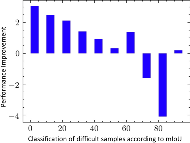
Figure 2: Analysis of samples with different difficulties. All categories are divided into difficult and easy samples according to the performance. The abscissa represents the difficulty of the category, which is becoming simpler and simpler from left to right. The ordinate represents a performance improvement.

Ablation study of $\lambda$. As shown in $\ell_{aug}^{CWD}$, there has $\lambda$ to adjust the ratio. However, since covariance is tunneled training process by data set statistics, it is less stable in the early stage of training. For stabilize training, $\lambda$ uses the cosine update method. As shown in Table 5 , we investigate the impact of $\lambda$ in our FAKD, and $\lambda=1.0$ is the best choice.

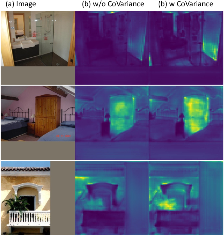
Figure 3: Visual of samples with or without co-variance. By augmenting the feature with co-variance, the activation of the meaningful region is strengthen.

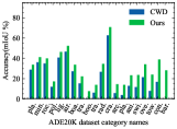
(a) ADE20K

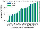
(b) Cityscapes

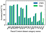
(c) Pascal Cotext

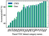
(d) Pascal VOC

Figure 4: Illustrations of the effectiveness of our methods in terms of class IoU scores using the network PSPnet-ResNet18. Both CWD and our method are helpful for improving the performance especially for the hard classes with low IoU scores. The improvement from our method is more significant for hard objects.

Ablation study of hard example mining. As shown in Figure 2, the item with $\Sigma$ in $\ell_{aug}^{CWD}$ and $\ell_{aug}^{PD}$ is reflected as a dynamically adjusted complex sample. So we divided the different difficult samples and analyzed the performance improvement for samples of different difficulties. From the results, it can be seen that our method can effectively improve the problematic samples. Also, we visualized the feature maps as Illustrated in Figure 3. It can also be seen from the feature map that adding our method enables the feature map to highlight some problematic regions more. Each class IoU score is shown in Figure 4.

Conclusion

This paper presents a novel feature augmented knowledge distillation (FAKD) method for semantic segmentation to increase the training samples for the student network in the feature space. Our method augments feature maps and constrains all augmented features with the teacher network. Experiments on four public segmentation datasets demonstrate the effectiveness of our FAKD. Our method also demonstrates superiority on long-tail problems. The performance for classes with less training samples has been improved with a larger margin. We hope our work inspires future research exploring semantic feature augmentation for knowledge distillation.

References

- Bengio et al. (2013) Bengio, Y.; Mesnil, G.; Dauphin, Y.; and Rifai, S. 2013. Better mixing via deep representations. In Proc. Int. Conf. Mach. Learn., 552–560. PMLR.
- Bertasius, Shi, and Torresani (2016) Bertasius, G.; Shi, J.; and Torresani, L. 2016. Semantic segmentation with boundary neural fields. In Proc. IEEE Conf. Comput. Vis. Pattern Recog., 3602–3610.
- Chen et al. (2016) Chen, L.-C.; Barron, J. T.; Papandreou, G.; Murphy, K.; and Yuille, A. L. 2016. Semantic image segmentation with task-specific edge detection using cnns and a discriminatively trained domain transform. In Proc. IEEE Conf. Comput. Vis. Pattern Recog., 4545–4554.
- Chen et al. (2017) Chen, L.-C.; Papandreou, G.; Kokkinos, I.; Murphy, K.; and Yuille, A. L. 2017. Deeplab: Semantic image segmentation with deep convolutional nets, atrous convolution, and fully connected crfs. IEEE TPAMI, 40(4): 834–848.
- Chen et al. (2018) Chen, L.-C.; Zhu, Y.; Papandreou, G.; Schroff, F.; and Adam, H. 2018. Encoder-decoder with atrous separable convolution for semantic image segmentation. In Proc. Eur. Conf. Comput. Vis., 801–818.
- Chen et al. (2019) Chen, W.; Gong, X.; Liu, X.; Zhang, Q.; Li, Y.; and Wang, Z. 2019. Fasterseg: Searching for faster real-time semantic segmentation. arXiv preprint arXiv:1912.10917.
- Contributors (2020) Contributors, M. 2020. MMSegmentation: OpenMMLab Semantic Segmentation Toolbox and Benchmark. https://github.com/open-mmlab/mmsegmentation.
- Cordts et al. (2016) Cordts, M.; Omran, M.; Ramos, S.; Rehfeld, T.; Enzweiler, M.; Benenson, R.; Franke, U.; Roth, S.; and Schiele, B. 2016. The cityscapes dataset for semantic urban scene understanding. In Proc. IEEE Conf. Comput. Vis. Pattern Recog., 3213–3223.
- Ding et al. (2019) Ding, H.; Jiang, X.; Liu, A. Q.; Thalmann, N. M.; and Wang, G. 2019. Boundary-aware feature propagation for scene segmentation. In Proc. Int. Conf. Comput. Vis., 6819–6829.
- Everingham et al. (2010) Everingham, M.; Van Gool, L.; Williams, C. K. I.; Winn, J.; and Zisserman, A. 2010. The Pascal Visual Object Classes (VOC) Challenge. Int. J. Comput. Vis., 88(2): 303–338.
- Fu et al. (2019) Fu, J.; Liu, J.; Tian, H.; Li, Y.; Bao, Y.; Fang, Z.; and Lu, H. 2019. Dual attention network for scene segmentation. In Proc. IEEE Conf. Comput. Vis. Pattern Recog., 3146–3154.
- Gal and Ghahramani (2015) Gal, Y.; and Ghahramani, Z. 2015. Bayesian convolutional neural networks with Bernoulli approximate variational inference. arXiv preprint arXiv:1506.02158.
- He et al. (2019) He, J.; Deng, Z.; Zhou, L.; Wang, Y.; and Qiao, Y. 2019. Adaptive pyramid context network for semantic segmentation. In Proc. IEEE Conf. Comput. Vis. Pattern Recog., 7519–7528.
- He et al. (2016) He, K.; Zhang, X.; Ren, S.; and Sun, J. 2016. Deep residual learning for image recognition. In Proc. IEEE Conf. Comput. Vis. Pattern Recog., 770–778.
- Heo et al. (2019) Heo, B.; Kim, J.; Yun, S.; Park, H.; Kwak, N.; and Choi, J. Y. 2019. A comprehensive overhaul of feature distillation. In Proc. Int. Conf. Comput. Vis., 1921–1930.
- Hinton, Vinyals, and Dean (2015) Hinton, G.; Vinyals, O.; and Dean, J. 2015. Distilling the knowledge in a neural network. arXiv preprint arXiv:1503.02531.
- Hou et al. (2020) Hou, Y.; Ma, Z.; Liu, C.; Hui, T.-W.; and Loy, C. C. 2020. Inter-region affinity distillation for road marking segmentation. In Proc. IEEE Conf. Comput. Vis. Pattern Recog., 12486–12495.
- Huang et al. (2019) Huang, Z.; Wang, X.; Huang, L.; Huang, C.; Wei, Y.; and Liu, W. 2019. Ccnet: Criss-cross attention for semantic segmentation. In Proc. Int. Conf. Comput. Vis., 603–612.
- Kendall and Gal (2017) Kendall, A.; and Gal, Y. 2017. What uncertainties do we need in bayesian deep learning for computer vision? Proc. Adv. Neural Inform. Process. Syst., 30.
- Li et al. (2019) Li, H.; Xiong, P.; Fan, H.; and Sun, J. 2019. Dfanet: Deep feature aggregation for real-time semantic segmentation. In Proc. IEEE Conf. Comput. Vis. Pattern Recog., 9522–9531.
- Li, Zuo, and Zhang (2016) Li, M.; Zuo, W.; and Zhang, D. 2016. Convolutional network for attribute-driven and identity-preserving human face generation. arXiv preprint arXiv:1608.06434.
- Lin et al. (2017) Lin, G.; Milan, A.; Shen, C.; and Reid, I. 2017. Refinenet: Multi-path refinement networks for high-resolution semantic segmentation. In Proc. IEEE Conf. Comput. Vis. Pattern Recog., 1925–1934.
- Liu et al. (2019) Liu, Y.; Chen, K.; Liu, C.; Qin, Z.; Luo, Z.; and Wang, J. 2019. Structured knowledge distillation for semantic segmentation. In Proc. IEEE Conf. Comput. Vis. Pattern Recog., 2604–2613.
- Liu et al. (2020) Liu, Y.; Shu, C.; Wang, J.; and Shen, C. 2020. Structured knowledge distillation for dense prediction. IEEE TPAMI.
- Long, Shelhamer, and Darrell (2015) Long, J.; Shelhamer, E.; and Darrell, T. 2015. Fully convolutional networks for semantic segmentation. In Proc. IEEE Conf. Comput. Vis. Pattern Recog., 3431–3440.
- Mehta et al. (2018) Mehta, S.; Rastegari, M.; Caspi, A.; Shapiro, L.; and Hajishirzi, H. 2018. Espnet: Efficient spatial pyramid of dilated convolutions for semantic segmentation. In Proc. Eur. Conf. Comput. Vis., 552–568.
- Mottaghi et al. (2014) Mottaghi, R.; Chen, X.; Liu, X.; Cho, N.-G.; Lee, S.-W.; Fidler, S.; Urtasun, R.; and Yuille, A. 2014. The Role of Context for Object Detection and Semantic Segmentation in the Wild. In Proc. IEEE Conf. Comput. Vis. Pattern Recog.
- Park et al. (2019) Park, W.; Kim, D.; Lu, Y.; and Cho, M. 2019. Relational knowledge distillation. In Proc. IEEE Conf. Comput. Vis. Pattern Recog., 3967–3976.
- Paszke et al. (2016) Paszke, A.; Chaurasia, A.; Kim, S.; and Culurciello, E. 2016. Enet A deep neural network architecture for real-time semantic segmentation. arXiv preprint arXiv:1606.02147.
- Peng et al. (2019) Peng, B.; Jin, X.; Liu, J.; Li, D.; Wu, Y.; Liu, Y.; Zhou, S.; and Zhang, Z. 2019. Correlation congruence for knowledge distillation. In Proc. Int. Conf. Comput. Vis., 5007–5016.
- Peng et al. (2017) Peng, C.; Zhang, X.; Yu, G.; Luo, G.; and Sun, J. 2017. Large kernel matters–improve semantic segmentation by global convolutional network. In Proc. IEEE Conf. Comput. Vis. Pattern Recog., 4353–4361.
- Qian, Li, and Hu (2022) Qian, Q.; Li, H.; and Hu, J. 2022. Improved Knowledge Distillation via Full Kernel Matrix Transfer. In Proc. SIAM Int. Conf. on Data Mining, 612–620. SIAM.
- Romero et al. (2014) Romero, A.; Ballas, N.; Kahou, S. E.; Chassang, A.; Gatta, C.; and Bengio, Y. 2014. Fitnets: Hints for thin deep nets. arXiv preprint arXiv:1412.6550.
- Shu et al. (2021) Shu, C.; Liu, Y.; Gao, J.; Yan, Z.; and Shen, C. 2021. Channel-Wise Knowledge Distillation for Dense Prediction. In Proc. Int. Conf. Comput. Vis., 5311–5320.
- Takikawa et al. (2019) Takikawa, T.; Acuna, D.; Jampani, V.; and Fidler, S. 2019. Gated-scnn: Gated shape cnns for semantic segmentation. In Proc. Int. Conf. Comput. Vis., 5229–5238.
- Upchurch et al. (2017) Upchurch, P.; Gardner, J.; Pleiss, G.; Pless, R.; Snavely, N.; Bala, K.; and Weinberger, K. 2017. Deep feature interpolation for image content changes. In Proc. IEEE Conf. Comput. Vis. Pattern Recog., 7064–7073.
- Wang et al. (2018) Wang, X.; Girshick, R.; Gupta, A.; and He, K. 2018. Non-local neural networks. In Proc. IEEE Conf. Comput. Vis. Pattern Recog., 7794–7803.
- Wang et al. (2021a) Wang, Y.; Huang, G.; Song, S.; Pan, X.; Xia, Y.; and Wu, C. 2021a. Regularizing deep networks with semantic data augmentation. IEEE TPAMI.
- Wang et al. (2019) Wang, Y.; Pan, X.; Song, S.; Zhang, H.; Huang, G.; and Wu, C. 2019. Implicit semantic data augmentation for deep networks. Proc. Adv. Neural Inform. Process. Syst., 32: 12635–12644.
- Wang et al. (2021b) Wang, Y.; Xu, Z.; Wang, X.; Shen, C.; Cheng, B.; Shen, H.; and Xia, H. 2021b. End-to-end video instance segmentation with transformers. In Proc. IEEE Conf. Comput. Vis. Pattern Recog., 8741–8750.
- Wang et al. (2020) Wang, Y.; Zhou, W.; Jiang, T.; Bai, X.; and Xu, Y. 2020. Intra-class feature variation distillation for semantic segmentation. In Proc. Eur. Conf. Comput. Vis., 346–362. Springer.
- Xie et al. (2021) Xie, E.; Wang, W.; Yu, Z.; Anandkumar, A.; Alvarez, J. M.; and Luo, P. 2021. SegFormer: Simple and Efficient Design for Semantic Segmentation with Transformers. Proc. Adv. Neural Inform. Process. Syst.
- Yang et al. (2022) Yang, C.; Zhou, H.; An, Z.; Jiang, X.; Xu, Y.; and Zhang, Q. 2022. Cross-image relational knowledge distillation for semantic segmentation. In Proc. IEEE Conf. Comput. Vis. Pattern Recog., 12319–12328.
- Yang et al. (2018) Yang, M.; Yu, K.; Zhang, C.; Li, Z.; and Yang, K. 2018. Denseaspp for semantic segmentation in street scenes. In Proc. IEEE Conf. Comput. Vis. Pattern Recog., 3684–3692.
- Yu et al. (2021) Yu, C.; Gao, C.; Wang, J.; Yu, G.; Shen, C.; and Sang, N. 2021. Bisenet v2: Bilateral network with guided aggregation for real-time semantic segmentation. Int. J. Comput. Vis., 129(11): 3051–3068.
- Yu et al. (2020) Yu, C.; Wang, J.; Gao, C.; Yu, G.; Shen, C.; and Sang, N. 2020. Context prior for scene segmentation. In Proc. IEEE Conf. Comput. Vis. Pattern Recog., 12416–12425.
- Yu et al. (2018a) Yu, C.; Wang, J.; Peng, C.; Gao, C.; Yu, G.; and Sang, N. 2018a. Bisenet: Bilateral segmentation network for real-time semantic segmentation. In Proc. Eur. Conf. Comput. Vis., 325–341.
- Yu et al. (2018b) Yu, C.; Wang, J.; Peng, C.; Gao, C.; Yu, G.; and Sang, N. 2018b. Learning a discriminative feature network for semantic segmentation. In Proc. IEEE Conf. Comput. Vis. Pattern Recog., 1857–1866.
- Yu and Koltun (2015) Yu, F.; and Koltun, V. 2015. Multi-scale context aggregation by dilated convolutions. arXiv preprint arXiv:1511.07122.
- Yuan et al. (2020a) Yuan, J.; Deng, Z.; Wang, S.; and Luo, Z. 2020a. Multi Receptive Field Network for Semantic Segmentation. In Proc. Winter Conf. Appl. Comput. Vis., 1883–1892. IEEE.
- Yuan, Chen, and Wang (2020) Yuan, Y.; Chen, X.; and Wang, J. 2020. Object-contextual representations for semantic segmentation. In Computer Vision–ECCV 2020: 16th European Conference, Glasgow, UK, August 23–28, 2020, Proceedings, Part VI 16, 173–190. Springer.
- Yuan et al. (2018) Yuan, Y.; Huang, L.; Guo, J.; Zhang, C.; Chen, X.; and Wang, J. 2018. Ocnet: Object context network for scene parsing. arXiv preprint arXiv:1809.00916.
- Yuan et al. (2020b) Yuan, Y.; Xie, J.; Chen, X.; and Wang, J. 2020b. Segfix: Model-agnostic boundary refinement for segmentation. In European Conference on Computer Vision, 489–506. Springer.
- Zagoruyko and Komodakis (2016) Zagoruyko, S.; and Komodakis, N. 2016. Paying more attention to attention: Improving the performance of convolutional neural networks via attention transfer. arXiv preprint arXiv:1612.03928.
- Zhang et al. (2018) Zhang, H.; Dana, K.; Shi, J.; Zhang, Z.; Wang, X.; Tyagi, A.; and Agrawal, A. 2018. Context encoding for semantic segmentation. In Proc. IEEE Conf. Comput. Vis. Pattern Recog., 7151–7160.
- Zhao et al. (2018a) Zhao, H.; Qi, X.; Shen, X.; Shi, J.; and Jia, J. 2018a. Icnet for real-time semantic segmentation on high-resolution images. In Proc. Eur. Conf. Comput. Vis., 405–420.
- Zhao et al. (2017) Zhao, H.; Shi, J.; Qi, X.; Wang, X.; and Jia, J. 2017. Pyramid scene parsing network. In Proc. IEEE Conf. Comput. Vis. Pattern Recog., 2881–2890.
- Zhao et al. (2018b) Zhao, H.; Zhang, Y.; Liu, S.; Shi, J.; Loy, C. C.; Lin, D.; and Jia, J. 2018b. Psanet: Point-wise spatial attention network for scene parsing. In Proc. Eur. Conf. Comput. Vis., 267–283.
- Zhen et al. (2020) Zhen, M.; Wang, J.; Zhou, L.; Li, S.; Shen, T.; Shang, J.; Fang, T.; and Quan, L. 2020. Joint semantic segmentation and boundary detection using iterative pyramid contexts. In Proc. IEEE Conf. Comput. Vis. Pattern Recog., 13666–13675.
- Zheng et al. (2021) Zheng, S.; Lu, J.; Zhao, H.; Zhu, X.; Luo, Z.; Wang, Y.; Fu, Y.; Feng, J.; Xiang, T.; Torr, P. H.; et al. 2021. Rethinking semantic segmentation from a sequence-to-sequence perspective with transformers. In Proc. IEEE Conf. Comput. Vis. Pattern Recog., 6881–6890.
- Zhong et al. (2020) Zhong, Z.; Lin, Z. Q.; Bidart, R.; Hu, X.; Daya, I. B.; Li, Z.; Zheng, W.-S.; Li, J.; and Wong, A. 2020. Squeeze-and-attention networks for semantic segmentation. In Proc. IEEE Conf. Comput. Vis. Pattern Recog., 13065–13074.
- Zhou et al. (2017) Zhou, B.; Zhao, H.; Puig, X.; Fidler, S.; Barriuso, A.; and Torralba, A. 2017. Scene parsing through ade20k dataset. In Proc. IEEE Conf. Comput. Vis. Pattern Recog., 633–641.
- Zhou et al. (2021) Zhou, H.; Song, L.; Chen, J.; Zhou, Y.; Wang, G.; Yuan, J.; and Zhang, Q. 2021. Rethinking soft labels for knowledge distillation: A bias-variance tradeoff perspective. arXiv preprint arXiv:2102.00650.
- Zhou et al. (2019) Zhou, Y.; Sun, X.; Zha, Z.-J.; and Zeng, W. 2019. Context-reinforced semantic segmentation. In Proc. IEEE Conf. Comput. Vis. Pattern Recog., 4046–4055.