Unit-length Rectangular Drawings of Graphs

Abstract

A rectangular drawing of a planar graph $G$ is a planar drawing of $G$ in which vertices are mapped to grid points, edges are mapped to horizontal and vertical straight-line segments, and faces are drawn as rectangles. Sometimes this latter constraint is relaxed for the outer face. In this paper, we study rectangular drawings in which the edges have unit length. We show a complexity dichotomy for the problem of deciding the existence of a unit-length rectangular drawing, depending on whether the outer face must also be drawn as a rectangle or not. Specifically, we prove that the problem is -complete for biconnected graphs when the drawing of the outer face is not required to be a rectangle, even if the sought drawing must respect a given planar embedding, whereas it is polynomial-time solvable, both in the fixed and the variable embedding settings, if the outer face is required to be drawn as a rectangle.

1 Introduction

Among the most celebrated aesthetic criteria in Graph Drawing we have: (i) planarity, (ii) orthogonality of the edges, (iii) unit length of the edges, and (iv) convexity of the faces. We focus on drawings in which all the above aesthetics are pursued at once. Namely, we study orthogonal drawings where the edges have length one and the faces are rectangular.

Throughout the paper, any considered graph drawing has the vertices mapped at distinct points of the plane. Orthogonal representations are a classic research topic in graph drawing. A rich body of literature is devoted to orthogonal drawings of planar [DBLP:journals/siamcomp/BattistaLV98, dlop-oodlt-20, DBLP:conf/gd/GargL99, DBLP:journals/siamdm/ZhouN08] and plane [DBLP:journals/jgaa/CornelsenK12, DBLP:journals/jgaa/RahmanNN99, DBLP:conf/wg/RahmanN02, DBLP:conf/stoc/Storer80, DBLP:journals/siamcomp/Tamassia87] graphs with the minimum number of bends in total or per edge [DBLP:journals/comgeo/BiedlK98, DBLP:journals/algorithmica/Kant96, DBLP:journals/dam/LiuMS98]. An orthogonal drawing with no bend is a rectilinear drawing. Several papers address rectilinear drawings of planar [DBLP:conf/compgeom/ChangY17, DBLP:conf/gd/Frati20, DBLP:journals/siamcomp/GargT01, DBLP:conf/cocoon/Hasan019, DBLP:conf/gd/RahmanEN05, DBLP:journals/ieicet/RahmanEN05] and plane [DBLP:conf/gd/Didimo0LO20, DBLP:conf/gd/Frati20, DBLP:journals/jgaa/RahmanNN03, DBLP:journals/siamcomp/VijayanW85] graphs. When all the faces of a rectilinear drawing have a rectangular shape the drawing is rectangular. Maximum degree-3 plane graphs admitting rectangular drawings were first characterized in [Th84, u-drm-53]. A linear-time algorithm to find a rectangular drawing of a maximum degree-$3$ plane graph, provided it exists, is described in [DBLP:journals/comgeo/RahmanNN98] and extended to maximum degree-$3$ planar graphs in [DBLP:journals/jal/RahmanNG04]. Surveys on rectangular drawings can be found in [f-rsrpg-13, DBLP:books/ws/NishizekiR04, nr-rda-13]. If only the internal faces are constrained to be rectangular, then the drawing is called inner-rectangular. In [mhn-irdpg-06] it is shown that a plane graph $G$ has an inner-rectangular drawing $\Gamma$ if and only if a special bipartite graph constructed from $G$ has a perfect matching. Also, $\Gamma$ can be found in $O(n^{1.5}/\log n)$ time if $G$ has $n$ vertices and a “sketch” of the outer face is prescribed, i.e., all the convex and concave outer vertices are prescribed.

Figure 1: Unit-length embedding-preserving rectangular drawings of a plane graph.

Computing straight-line drawings whose edges have constrained length is another core topic in graph drawing [DBLP:conf/compgeom/AbelDDELS16, DBLP:conf/gd/AlegriaBLBFP21, DBLP:conf/gd/AngeliniLBBHPR14, DBLP:conf/alenex/0001S20, cdr-pegse-07, DBLP:journals/dam/EadesW90, Schaefer2013]. The graphs admitting planar straight-line drawings with all edges of the same length are also called matchstick graphs. Recognizing matchstick graphs is -hard for biconnected [DBLP:journals/dam/EadesW90] and triconnected [cdr-pegse-07] graphs, and in fact, even strongly $\exists\mathbb{R}$-complete [DBLP:conf/compgeom/AbelDDELS16]; see also [Schaefer2013].

A unit-length grid drawing maps vertices to grid points and edges to horizontal or vertical segments of unit Euclidean length. A grid graph is a graph that admits a unit-length grid drawing. Recognizing grid graphs is -complete for ternary trees of pathwidth $3$ [DBLP:journals/ipl/BhattC87], for binary trees [g-ulebt-89], and for trees of pathwidth $2$ [gsz-grcpc-21], but solvable in polynomial time on graphs of pathwidth $1$ [gsz-grcpc-21]. An exponential-time algorithm to compute, for a given weighted planar graph, a rectilinear drawing in which the Euclidean length of each edge is equal to the edge weight has been presented in [DBLP:conf/alenex/0001S20].

Let $G$ be a planar graph. The Unit-length Inner-Rectangular Drawing Recognition (for short, UIR) problem asks whether a unit-length inner-rectangular drawing of $G$ exists. Similarly, the Unit-length Rectangular Drawing Recognition (for short, UR) problem asks whether a unit-length rectangular drawing of $G$ exists. Let now $H$ be a plane or planar embedded (i.e., no outer face specified) graph. The Unit-length Inner-Rectangular Drawing Recognition with Fixed Embedding (for short, UIRFE) problem asks whether a unit-length inner-rectangular embedding-preserving drawing of $H$ exists. Similarly, the Unit-length Rectangular Drawing Recognition with Fixed Embedding (for short, URFE) problem asks whether a unit-length rectangular embedding-preserving drawing of $H$ exists; see Fig. 1.

Our contribution.

In Sect. 3 we show -completeness for the UIRFE and UIR problems when the input graph is biconnected, which is surprising since a biconnected graph has degrees of freedom that are more restricted than those of a tree. In Sect. 4 we provide a linear-time algorithm for the UIRFE and URFE problems if the drawing of the outer face is given. In Sect. 5 we first show that the URFE problem is cubic-time solvable; the time bound becomes linear if all internal faces of the input graph have maximum degree $6$. These results hold both when the outer face is prescribed and when it is not. Second, we show a necessary condition for an instance of the UR problem to be positive in terms of its SPQR-tree. Exploiting the above condition, we show that the UR problem is cubic-time solvable; the running time becomes linear when the SPQR-tree of the input graph satisfies special conditions. Finally, as a by-product of our research, we provide the first polynomial-time algorithm to test whether a planar graph $G$ admits a rectangular drawing, for general instances of maximum degree $4$.

Full details for the proofs of the statements marked with a $(\star)$ are in the appendix.

2 Preliminaries

For basic graph drawing terminology and definitions refer, e.g., to [DBLP:books/ph/BattistaETT99, DBLP:books/ws/NishizekiR04].

(a)

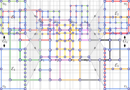
(b)

Figure 2: 2(a) A planar rectilinear grid drawing of a graph. 2(b) A unit-length rectangular grid drawing of the same graph.

Drawings and embeddings.

Two planar drawings of a connected graph are planar equivalent if they induce the same counter-clockwise ordering of the edges incident to each vertex. Also, they are plane equivalent if they are planar equivalent and the clockwise order of the edges along the boundaries of their outer faces is the same. The equivalence classes of planar equivalent drawings are called planar embeddings, whereas the equivalence classes of plane equivalent drawings are called plane embeddings. A planar embedded graph is a planar graph equipped with one of its planar embeddings. Similarly, a plane graph is a planar graph equipped with one of its plane embeddings. Given a planar embedded (resp. plane) graph $G$ and a planar (resp. plane) embedding $\mathcal{E}$ of $G$, a planar drawing $\Gamma$ of $G$ is embedding-preserving if $\Gamma\in\mathcal{E}$.

2.1 Geometric definitions for Lemma 2

A polygon is a closed polygonal chains consisting of a finite number of straight-line segments. A polygon intersect itself if two segments non-adjacent in the chain have a non-void intersection. A polygon is simple if it does not intersect itself. This implies that there are no repeated segments or points in the chain. A polygon is weakly simple if its bounds a region of the plane that is homeomorphic to a an open disk. A simple polygon is convex if its interior is a convex set. A convex drawing of a planar graph $G$ is a straight-line planar drawing of $G$ in which all the faces are drawn as convex polygons, including the outer face. In [DBLP:journals/iandc/BattistaTV01], it has been shown that a planar graph admits a convex drawing only if it is biconnected. A convex subdivision of a simple polygon $P$ is partition of the interior of $P$ into convex sets. Note that, a convex drawing defines a convex subdivision of the polygon bounding the outer face. In a grid drawing, vertices are mapped to points with integer coordinates (i.e., grid points). A drawing of a graph in which all edges have unit Euclidean length is a unit-length drawing (see Fig. 2 for an example).

Observation 1.

A unit-length grid drawing is rectilinear and planar.

Observation 2.

A unit-length rectangular (or inner-rectangular) drawing is planar and it is a grid drawing, up to a rigid transformation.

The following simple property has been proved in [10.1007/s11227-016-1811-y, Lemma 1].

Property 1.

Every cycle that admits a unit-length grid drawing has even length.

Since (inner) rectangular drawings exist only for maximum-degree-$4$ graphs, in the remainder, we assume that all considered graphs satisfy this requirement.

Connectivity.

A biconnected component (or block) of a graph $G$ is a maximal (in terms of vertices and edges) biconnected subgraph of $G$. A block is trivial if it consists of a single edge and non-trivial otherwise. A split pair of $G$ is either a pair of adjacent vertices or a separation pair, i.e., a pair of vertices whose removal disconnects $G$. The components of $G$ with respect to a split pair $\{u,v\}$ are defined as follows. If $(u,v)$ is an edge of $G$, then it is a component of $G$ with respect to $\{u,v\}$. Also, let $G_{1},\dots,G_{k}$ be the connected components of $G\setminus\{u,v\}$. The subgraphs of $G$ induced by $V(G_{i})\cup\{u,v\}$, minus the edge $(u,v)$, are components of $G$ with respect to $\{u,v\}$, for $i=1,\dots,k$. Due to space limitations, we refer the reader to Sect. 2.2 and to [DBLP:journals/algorithmica/BattistaT96, dt-opl-96] for the definition of SPQR-tree.

2.2 SPQR-trees

We provide details of the SPQR-tree data structure introduced by Di Battista and Tamassia [DBLP:journals/algorithmica/BattistaT96, dt-opl-96] to handle all planar embeddings of a biconnected planar graph $H$. The SPQR-tree $T$ of $H$ represents a decomposition of $H$ into triconnected components along its split pairs. Each node $\mu$ of $T$ contains a graph, called skeleton of $\mu$, and denoted $\operatorname{sk}(\mu)$. The edges of $\operatorname{sk}(\mu)$ are either edges of $H$, which we call real edges, or newly introduced edges, called virtual edges. The tree $T$ is initialized to a single node $\mu$, whose skeleton, composed only of real edges, is $H$. Consider a split pair $\{u,v\}$ of the skeleton of some node $\mu$ of $T$, and let $H_{1},\dots,H_{k}$ be the components of $H$ with respect to $\{u,v\}$ such that $H_{1}$ is not a virtual edge and, if $k=2$, also $H_{2}$ is not a virtual edge. We introduce a node $\nu$ adjacent to $\mu$ whose skeleton is the graph $H_{1}+e_{\nu,\mu}$, where $e_{\nu,\mu}=(u,v)$ is a virtual edge, and replace $\operatorname{sk}(\mu)$ with the graph $\bigcup_{i\neq 1}H_{i}+e_{\mu,\nu}$, where $e_{\mu,\nu}=(u,v)$ is a virtual edge. We say that $e_{\nu,\mu}$ is the twin virtual edge of $e_{\mu,\nu}$, and vice versa. Applying this replacement iteratively produces a tree with more nodes but smaller skeletons associated with the nodes. Eventually, when no further replacement is possible, the skeletons of the nodes of $T$ are of four types: parallels of at least three virtual edges ($P$-nodes), parallels of exactly one virtual edge and one real edge ($Q$-nodes), cycles of exactly three virtual edges ($S$-nodes), and triconnected planar graphs ($R$-nodes). The merge of two adjacent nodes $\mu$ and $\nu$ in $T$, replaces $\mu$ and $\nu$ in $T$ with a new node $\tau$ that is adjacent to all the neighbors of $\mu$ and $\nu$, and whose skeleton is $\operatorname{sk}(\mu)\cup\operatorname{sk}(\nu)\setminus\{e_{\mu,\nu},e_{\nu,\mu}\})$, where the end-vertices of $e_{\mu,\nu}$ and $e_{\nu,\mu}$ that correspond to the same vertices of $H$ are identified. By iteratively merging adjacent $S$-nodes, we eventually obtain the (unique) SPQR-tree data structure as introduced by Di Battista and Tamassia [DBLP:journals/algorithmica/BattistaT96, dt-opl-96], where the skeleton of an $S$-node is a cycle. The crucial property of this decomposition is that a planar embedding of $H$ uniquely induces a planar embedding of the skeletons of its nodes and that, arbitrary and independently, choosing planar embeddings for all the skeletons uniquely determines an embedding of $H$. Observe that the skeletons of $S$- and $Q$-nodes have a unique planar embedding, that the skeleton of $R$-nodes have two planar embeddings (which are one the mirror of the other), and that $P$-nodes have as many planar embedding as the permutations of their virtual edges. Consider a node $\mu$ and a virtual edge $e_{\nu,\mu}$ in $\operatorname{sk}(\mu)$. Let $T_{\nu,\mu}$ be the subtree of $T$ obtained by removing the arc $(\nu,\mu)$ from $T$ and contains $\nu$. The expansion graph of $e_{\nu,\mu}$ is the subgraph of $H$ obtained by iteratively merging all the node in $T_{\nu,\mu}$ and by removing the virtual edge $e_{\mu,\nu}$.

It is often convenient to orient the arcs of $T$ so that, in the resulting directed tree, one $Q$-node $\rho$ is a sink and all other nodes have exactly one outgoing arc. Such an orientation corresponds to rooting $T$ at $\rho$, and we call it a normal orientation of $T$. The next definitions assume a normal orientation of $T$. For a node $\mu\neq\rho$ of $T$, the poles of $\mu$ are the endpoints of the virtual edge $e_{\nu,\mu}$ of $\operatorname{sk}(\mu)$ where $\nu$ is the parent of $\mu$; whereas the poles of $\rho$ are the endpoints of its unique virtual edge. Note that, any plane embedding $\cal E$ of $H$, in which the real edge corresponding to $\rho$ is incident to the outer face, yields a plane embedding $\mathcal{E}_{\mu}$ of the skeleton of each node $\mu$ of $T$ in which the poles of $\mu$ are also incident to the outer face of $\mathcal{E}_{\mu}$. This motivates the next definitions. Consider a node $\mu$. Also, let $u$ and $v$ be the poles of $\mu$. Let $\nu$ be the parent of $\mu$ and let $e_{\mu,\nu}$ be the virtual edge representing $\mu$ in $\operatorname{sk}(\nu)$. Let $\mathcal{E}_{\mu}$ be the restriction of $\mathcal{E}$ to $\exp{(e_{\mu,\nu})}$ and let $H_{\mu}$ be the corresponding plane graph. Note that, there exist exactly two faces of $\mathcal{E}_{\mu}$ that are incident to edges of the outer face of $H_{\mu}$. We call such faces the outer faces of $\mathcal{E}_{\mu}$. By convention, we call left outer face $\ell(\mathcal{E}_{\mu})$ of $\mathcal{E}_{\mu}$ (right outer face $r(\mathcal{E}_{\mu})$ of $\mathcal{E}_{\mu}$) the outer face that is delimited by the path obtained by walking in clockwise direction (resp. in counter-clockwise direction) from $u$ to $v$ along the boundary of the outer face of $\mathcal{E}_{\mu}$. The terms left outer face and right outer face come from the fact that we usually think about $\mathcal{E}_{\mu}$ as having the pole $u$ at the bottom and the other pole $v$ at the top.

If $H$ has $n$ vertices, then $T$ has $O(n)$ nodes and the total number of virtual edges in the skeletons of the nodes of $T$ is in $O(n)$. From a computational complexity perspective, $T$ can be constructed in $O(n)$ time [DBLP:conf/gd/GutwengerM00].

3 NP-completeness of the UIRFE and UIR problems

In this section we show -completeness for both the UIRFE and UIR problems when the input graph is biconnected. We start with the following theorem.

Theorem 3.1.

The UIRFE problem is -complete, even for biconnected plane graphs whose internal faces have maximum size $6$.

Let $\phi$ be a Boolean formula in conjunctive normal form with at most three literals in each clause. We denote by $G_{\phi}$ the incidence graph of $\phi$, i.e., the graph that has a vertex for each clause of $\phi$, a vertex for each variable of $\phi$, and an edge $(c,v)$ for each clause $c$ that contains the positive literal $v$ or the negated literal $\overline{v}$. The formula $\phi$ is an instance of Planar Monotone 3-SAT if $G_{\phi}$ is planar and each clause of $\phi$ is either positive or negative. A positive clause contains only positive literals, while a negative clause contains only negated literals. Hereafter, w.l.o.g., we assume that all the clauses of $\phi$ contain exactly three literals.

A monotone rectilinear representation of $G_{\phi}$ is a drawing that satisfies the following properties (refer to Fig. 3(a)). P1: Variables and clauses are represented by axis-aligned rectangles with the same height. P2: The bottom sides of all rectangles representing variables lie on the same horizontal line. P3: The rectangles representing positive (resp. negative) clauses lie above (resp. below) the rectangles representing variables. P4: Edges connecting variables and clauses are represented by vertical segments. P5: The drawing is crossing-free.

The Planar Monotone 3-SAT problem is known to be -complete, even when the incidence graph $G_{\phi}$ of $\phi$ is provided along with a monotone rectilinear representation $\Gamma_{\phi}$ of $G_{\phi}$ [10.1142/S0218195912500045]. We prove Theorem 3.1 by showing how to construct a plane graph $H_{\phi}$ that is biconnected, has internal faces of maximum size $6$, and admits a unit-length inner-rectangular drawing if and only if $\phi$ is satisfiable. Our strategy is to modify $\Gamma_{\phi}$ to create a suitable auxiliary representation $\Gamma^{*}_{\phi}$ (see Fig. 3) and then to use the geometric information of $\Gamma^{*}_{\phi}$ as a blueprint to construct $H_{\phi}$. Because of the lack of space, we describe in detail how to obtain $\Gamma^{*}_{\phi}$ from $\Gamma_{\phi}$ in Sect. 3.1, and how to construct $H_{\phi}$ in Sects. 3.2 and 3.3. We provide below a high-level description of the logic behind the reduction.

(a) $\Gamma_{\phi}$

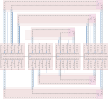
(b) $\Gamma^{*}_{\phi}$

Figure 3: 3(a) The monotone rectilinear representations $\Gamma_{\phi}$ of $G_{\phi}$. The rectangles representing variables and clauses are red, whereas the line segments and rectangles representing the edges of $\phi$ are blue. 3(b) The auxiliary representation $\Gamma^{*}_{\phi}$.

3.1 The auxiliary monotone rectilinear representation $\Gamma^{*}_{\phi}$

Hereafter, let $\delta^{+}_{\phi}$ (resp. $\delta^{-}_{\phi}$) be the maximum degree of $G_{\phi}$ when restricted to nodes representing variables and positive (resp. negative) clauses. Let $\delta_{\phi}=\max(\delta^{+}_{\phi},\delta^{-}_{\phi})$. The auxiliary representation has the following properties (refer to Fig. 3):

1. The variables, clauses, and edges of $G_{\phi}$ are represented by axis-aligned rectangles whose corners have integer coordinates, i.e., they lie at grid points.

2. The width and height of the bounding box of $\Gamma^{*}_{\phi}$ are polynomially bounded in the size of $\phi$.

3. The rectangles representing variables have width $16\delta_{\phi}+9$, height $76$, and their bottom sides lie on a common horizontal grid line.

4. The rectangles representing clauses have width equal to an odd integer greater than $85$, and height equal to $22$.

5. The rectangles representing edges have width equal to $6$, and height equal to a even integer greater than $6$.

6. Consider the rectangle $\mathcal{R}$ representing a variable $v\in\phi$, and the set $\mathcal{S}$ of rectangles incident to $\mathcal{R}$ that represent the edges of $G_{\phi}$ incident to $v$. Each rectangle of $\mathcal{S}$ has horizontal distance from the (vertical) right side of $\mathcal{R}$ that is a multiple of $2$.

7. Consider the rectangle $\mathcal{R}$ representing a positive (resp. negative) clause $c\in\phi$. Let $s_{1}$, $s_{2}$, and $s_{3}$ be the intersection segments between the rectangles representing the edges of $G_{\phi}$ incident to $c$, and the bottom (resp. top) horizontal side of $\mathcal{R}$. The left endpoint of $s_{1}$ lies on the bottom-left (resp. top-left) corner of $\mathcal{R}$, the right endpoint of $s_{3}$ lies on the bottom-right (resp. top-right) corner of $\mathcal{R}$, and the horizontal distances between $s_{1}$ and $s_{2}$ and between $s_{2}$ and $s_{3}$, are even numbers greater than or equal to $12$.

We can obtain $\Gamma^{*}_{\phi}$ by suitable translation and scaling of the rectangles that represent the variables, clauses, and edges of $\phi$ in $\Gamma_{\phi}$. Clearly, these transformations can be done in polynomial time in the size of $\phi$. We obtain the following lemma.

Lemma 1.

Starting from $\Gamma_{\phi}$, the representation $\Gamma^{*}_{\phi}$ can be constructed in polynomial time in the size of $\phi$.

Figure 4: The graph $H_{\phi}$. Variable and clause gadgets are enclosed in light red boxes, while transmission gadgets are enclosed in light blue boxes.

3.1.1 Overview of the reduction.

The reduction is based on three main types of gadgets. A variable $v\in\phi$ is modeled by means of a variable gadget, a clause $c\in\phi$ by means of an $(\alpha,\beta)$-clause gadget, and an edge $(v,c)\in G_{\phi}$ by means of a $\lambda$-transmission gadget. We use the geometric properties of $\Gamma_{\phi}^{*}$ to determine the size and structure of each gadget, as well as how to combine the gadgets together to form $H_{\phi}$. The width and height of the rectangles representing variables, clauses, and edges are used to construct variable gadgets and to compute the auxiliary parameters $\alpha$, $\beta$ and $\lambda$, which in turn are used to construct $(\alpha,\beta)$-clause gadgets and $\lambda$-transmission gadgets. Finally, the incidences between the rectangles are used to decide how to join the gadgets to construct a single connected graph.

An example of a unit-length inner-rectangular drawing of $H_{\phi}$ is shown in Fig. 4; some faces of $H_{\phi}$ are omitted. All these missing faces are part of domino components, which admit a constant number of unit-length inner-rectangular drawings, see Fig. 5; some of these faces are shown filled in white or blue in Fig. 4.

(a) L-shape

(b) C-shape

(c) Stick

Figure 5: The unit-length grid drawings of the domino components. Domino component faces are filled blue (size $6$) and white (size $4$).

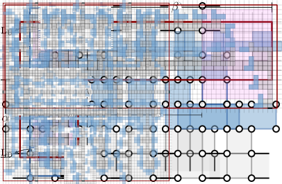
(a) A true configuration.

(b) A false configuration

Figure 6: The variable gadget.

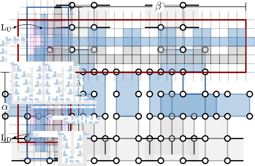
Figure 7: In every unit-length inner-rectangular drawing of an $(\alpha,\beta)$-clause gadget, at least one L-shape domino component crosses the red rectangle.

The logic behind the construction is as follows. A variable gadget admits two unit-length inner-rectangular drawings (see Fig. 6), which differ from each other on whether the domino components of the gadget stick out of the bottom or top side of the red enclosing rectangle, and correspond to a true/false assignment for the associated variable, respectively. The truth assignments are propagated from variable to clause gadgets via $\lambda$-transmission gadgets. A domino component sticking out of a variable gadget invades a transmission gadget, which causes a domino component at the other end of the transmission gadget to be directed towards the incident $(\alpha,\beta)$-clause gadget. The clause gadget is designed so that it admits a unit-length inner-rectangular drawing if and only if at least one of the extremal domino components of its three incident transmission gadgets is not directed towards it; this allows a domino component of the clause gadget to invade the transmission gadget and save space inside the clause gadget; see Fig. 7.

3.2 Description of the gadgets

All the gadgets have internal faces of size either $4$ or $6$, and are formed by two sets of special subgraphs we call the frames and the domino components. A frame is a biconnected subgraph formed by internal faces of size $4$, and has a unique unit-length inner-rectangular drawing (up to rigid transformations). A domino component is instead a biconnected subgraph with internal faces of size either $4$ or $6$. We define three different types of domino components: the L-shape, the C-shape, and the Stick. In all the gadgets, the adjacencies between the domino components and the frames force the L-shape and the C-shape components to have one out of two unit-length inner-rectangular drawings (shown in Fig. 5(a) and Fig. 5(b)), whereas the stick component is forced to have one out of three unit-length inner-rectangular drawings (shown in Fig. 5(c)).

Variable Gadget.

Variable gadgets are formed by $2\delta_{\phi}+2$ frames connected together by means of C-shape components, and a set of L-shape and stick components to propagate the truth assignment of the corresponding variable. Refer to Fig. 6 for an illustration of the gadget.

Let $\mathcal{V}$ denote the variable gadget modeling some variable $v\in\phi$. There are three crucial properties of the variable gadget. First, C-shape components are adjacent to frames in such a way, that in every unit-length inner-rectangular drawing of $\mathcal{V}$ the drawing of its frames is the same. This implies that the bounding box $\mathcal{B}$ of the drawing of the frames of $\mathcal{V}$ does not change, regardless of the drawings of the C-shape components. Second, $\mathcal{V}$ admits two unit-length inner-rectangular drawings that we associate with the true (Fig. 6(a)) and false (Fig. 6(b)) truth assignments of $v$. We remark that in the drawing corresponding to the true (resp. false) assignment, there are $\delta_{\phi}$ L-shape components crossing the bottom (resp. top) side of $\mathcal{B}$. Finally, the gadget is constructed in such a way, that the width and height of $\mathcal{B}$ are the same as those of the rectangle of $\Gamma_{\phi}^{*}$ representing $v$.

$\lambda$-transmission Gadget.

The $\lambda$-transmission gadget is formed by a single frame, and a set of $\lfloor(\lambda-2)/4\rfloor$ L-shape components to propagate truth assignments from variable to clause gadgets. Refer to Fig. 8 for an illustration of the gadget.

Let $\mathcal{L}$ denote the $\lambda$-transmission gadget modeling some edge $(v,c)$ of $G_{\phi}$ that connects a variable $v$ to a clause $c$. Consider the auxiliary purple rectangle $R$, and the L-shape components labeled with $L_{D}$ and $L_{U}$ in Fig. 8. There are two crucial properties of the $\lambda$-transmission gadget. First, in any unit-length inner-rectangular drawing of $\mathcal{L}$, if $L_{D}$ does not cross $R$ then $L_{U}$ crosses $R$, and vice versa. Observe that, if an L-shape component of a variable gadget crosses the top (resp. bottom) side of the red enclosing rectangle, then $L_{U}$ (resp. $L_{D}$) crosses $R$. This is how the truth assignment for a variable gets propagated through transmission gadgets. Second, the width and height of the bounding box $\mathcal{B}$ of all the unit-length inner-rectangular drawings of $\mathcal{L}$ are the same. Moreover, the width and height of $\mathcal{B}$ are less than or equal to the width and height of the rectangle of $\Gamma^{*}_{\phi}$ representing $(v,c)$.

Figure 8: Unit-length inner-rectangular drawings of a $\lambda$-transmission gadget for $\lambda=22$. 8 If $L_{D}$ does not cross the purple rectangle, then $L_{U}$ crosses the purple rectangle. 8 If $L_{U}$ does not cross the purple rectangle, then $L_{D}$ crosses the purple rectangle.

$(\alpha,\beta)$-clause Gadget.

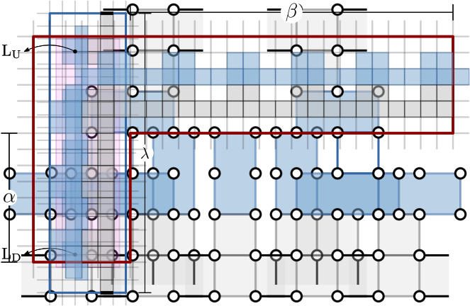
(a) The gadget admits no unit-length inner-rectangular drawing in which no L-shape component crosses the red rectangle.

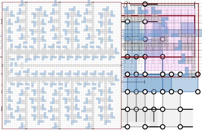
(b) The gadget admits a unit-length inner-rectangular drawing in which at least one L-shape component crosses the red rectangle.

Figure 9: The $(\alpha,\beta)$-clause gadget.

In the following, please refer to the example drawings of an $(\alpha,\beta)$-clause gadget shown in Fig. 9. Let $\mathcal{C}$ denote the $(\alpha,\beta)$-clause gadget modeling a clause $c\in\phi$. Let $R$ denote the auxiliary purple rectangle shown in Fig. 9. The gadget $\mathcal{C}$ is formed by three disconnected components. Each component is formed by a frame that, in the final graph $H_{\phi}$, is connected to the frame of a $\lambda$-transmission gadget modeling an edge of $G_{\phi}$ incident to $c$. The components are also equipped with L-shape components to propagate the truth assignments coming from $\lambda$-transmission gadgets.

Consider for the moment the three connected subgraphs of $\mathcal{C}$ that admit a unit-length inner-rectangular drawing lying outside $R$. Note they are straightforward extensions of $\lambda$-transmission gadgets. These auxiliary gadgets are used to propagate to $R$ the truth assignments coming from the boundary of the red enclosing rectangle. Each auxiliary gadget has the property that, in any unit-length inner-rectangular drawing, if no L-shape component crosses the red enclosing rectangle, then there is one L-shape component crossing $R$.

Consider now the subgraphs of $\mathcal{C}$ that admit a unit-length inner-rectangular drawing lying in the interior of $R$. The logic of the gadget is implemented by these subgraphs via the following crucial property: $\mathcal{C}$ admits a unit-length inner-rectangular drawing if and only if, at least one L-shape component of the auxiliary gadgets is not crossing $R$. See for example Fig. 9(a) in which all the three L-shape components of the auxiliary gadgets are crossing $R$, hence the $(\alpha,\beta)$-clause gadget does not admit a unit-length inner-rectangular drawing.

3.3 Combining the gadgets together to form $H_{\phi}$

For the purpose of combining two gadgets into a single connected graph, every gadget provides a set of special edges called attachment edges. In Figs. 6, 9 and 8, the attachment edges are shown as thick back segments. To combine two gadgets together, we first identify one attachment edge in each gadget, and then join the attachment edges together so there is a single edge shared by both gadgets.

In the following description, the properties D1-D7 of $\Gamma^{*}_{\phi}$ are exploited to guarantee that, after combining all the gadgets, $H_{\phi}$ admits a unit-length inner-rectangular drawing if and only if $\phi$ is satisfiable. To construct $H_{\phi}$ we start by constructing the variable gadgets using the parameter $\delta_{\phi}$ as we described above. The variable gadgets are connected together by means of frames whose dual graph is a path of length $7$. These frames are combined with the variable gadgets by means of the attachment edges lying on the right and the left sides of its red enclosing rectangle. The process continues by constructing an $\lambda$-transmission gadget per each edge of $G_{\phi}$. The value of the parameter $\lambda$ of each gadget is the height of the blue rectangle of $\Gamma_{\phi}^{*}$ representing the associated edge of $G_{\phi}$. A $\lambda$-transmission gadget and a variable gadget are combined together joining an attachment edge lying on the top (resp. bottom) side of the red enclosing rectangle of the variable gadget, and the attachment edge lying on the bottom (resp. top) side of the blue enclosing rectangle of the $\lambda$-transmission gadget. We finally construct an $(\alpha,\beta)$-clause gadget per each clause of $\phi$. We select the parameters $\alpha$ and $\beta$ according to the width of the red rectangles representing clauses in $\Gamma_{\phi}^{*}$, and the horizontal distances between the blue rectangles representing the edges incident to the modeled clause. A $\lambda$-transmission gadget and an $(\alpha,\beta)$-clause gadget are combined together joining an attachment edge lying on the bottom (resp. top) side of the red enclosing rectangle of the $(\alpha,\beta)$-clause gadget, and the attachment edge lying on the top (resp. bottom) side of the blue enclosing rectangle of the $\lambda$-transmission gadget.

By the construction described above, it is not hard to see that $H_{\phi}$ is biconnected and admits a unit-length inner-rectangular drawing that preserves the given plane embedding if and only if $\phi$ is satisfiable. The crucial property is that the domino components we use are forced to admit a constant number of unit-length inner-rectangular drawings that are all embedding preserving; see again Fig. 5.

By showing that, the graph $H_{\phi}$ only admits unit-length inner-rectangular drawings that preserve the same plane embedding, we get the following.

By showing that all the unit-length inner-rectangular drawings of $H_{\phi}$ respect the same plane embedding, we prove the following theorem.

[$\star$] The UIR problem is -complete, even for biconnected plane graphs whose internal faces have maximum size $6$.

Proof.

We show that the graph $H_{\phi}$ only admits unit-length inner-rectangular drawings that preserve the same plane embedding.

Let $\Gamma$ and $\Gamma^{\prime}$ be two unit-length inner-rectangular drawings of $H_{\phi}$. By construction, every edge of $H_{\phi}$ belongs to at least a length-$4$ or a length-$6$ chordless cycle. Each such a cycle must necessarily bound an internal face of $\Gamma$ and $\Gamma^{\prime}$. Therefore, the cycle bounding the outer face of $\Gamma$ and $\Gamma^{\prime}$ is the same. Let us call these cycles the inner cycles of $H_{\phi}$. Moreover, by construction, any of inner cycle shares at least an edge with an other inner cycle. Therefore, the orientation of the inner cycles is the same in $\Gamma$ as in $\Gamma^{\prime}$ (up to a mirroring of the entire drawing). Therefore, all the unit-length inner-rectangular drawings admitted by $H_{\phi}$ preserve the plane same embedding, which is unique up to reflections of the whole drawing.     ∎

4 An Algorithm for the UIRFE and URFE Problems with a Prescribed Drawing of the Outer Face

We start with two auxiliary lemmata. The first one is an extension of a classical result by Devillers et al. [10.1016/S0925-7721(98)00039-X].

Lemma 2.

Let $G$ be a connected planar graph and $\cal E$ be a plane embedding of $G$. A straight-line drawing $\Gamma$ of $G$ is planar and respects $\cal E$ if and only if:

• for every face $f$ of $\mathcal{E}$, the walk delimiting $f$ is represented in $\Gamma$ by a weakly simple polygon, whose orientation is as prescribed by $\mathcal{E}$;

• for every vertex $v$ of $G$, the clockwise order of the edges incident to $v$ in $\Gamma$ is the same as in $\mathcal{E}$; and

• let $C_{o}$ be the walk delimiting the outer face $f_{o}$ of $\mathcal{E}$, and let $\Gamma_{o}$ be the weakly simple polygon representing $C_{o}$ in $\Gamma$; then every edge not in $C_{o}$ that is incident to a vertex $v$ of $C_{o}$, leaves $v$ towards the interior of $\Gamma_{o}$.

Proof.

The necessity is obvious. We prove the sufficiency.

Denote by $\rho_{h}:=3n-h-3$ the number of edges of an internally-triangulated $n$-vertex graph whose outer face contains $h$ vertices (counting multiplicities). Let $k$ be the number of vertices of the convex hull of $\Gamma_{o}$. We prove the lemma by induction on $\rho_{k}-|E(G)|$.

If $\rho_{k}-|E(G)|=0$, then each internal face of $\cal E$ is a $3$-cycle and $f_{o}$ is a $k$-cycle. Since (i) each internal face of $\cal E$ is represented in $\Gamma$ by a triangle, and $f_{o}$ is represented in $\Gamma$ by a convex $k$-gon, and since (ii) the clockwise order of the edges incident to each vertex in $\Gamma$ is as prescribed by $\cal E$, a classic result by Devillers et al. [10.1016/S0925-7721(98)00039-X, Lemma 19] implies that $\Gamma$ is planar and induces a convex subdivision $\Gamma$ of $\Gamma_{o}$ (that also respects the planar embedding of $G$ obtained by disregarding the choice of the outer face of $\cal E$). Finally, the fact that $G$ is connected and that every edge not in $C_{o}$ that is incident to a vertex of $C_{o}$ leaves this vertex toward the interior of $\Gamma_{o}$ implies that $\Gamma_{o}$ bounds the outer face of $\Gamma$, and thus $\Gamma$ respects (the plane embedding) $\cal E$.

Let us now consider the case in which $\rho_{k}-|E(G)|>0$. Let $f$ be a face of $\cal E$ such that either $f$ is an internal face of $\cal E$ of length at least $3$ or $f=f_{o}$ if the polygon bounding $f_{o}$ in $\Gamma$ is not convex. Then, it is possible to draw in $\Gamma_{f}$ a straight-line segment $\overline{uv}$ between some pair of vertices $u$ and $v$ of $f$, such that $\overline{uv}$ does not cross any edge of $\Gamma_{f}$. In particular, $\overline{uv}$ divides $\Gamma_{f}$ into two weakly simple polygons $\Gamma_{f^{\prime}}$ and $\Gamma_{f^{\prime\prime}}$. Let $G^{\prime}$ be the planarly embedded graph obtained from $G$ by introducing the edge $(u,v)$ so that it splits $f$ into two faces $f^{\prime}$ and $f^{\prime\prime}$. Note that, by construction, $\Gamma_{f^{\prime}}$ and $\Gamma_{f^{\prime\prime}}$ bound $f^{\prime}$ and $f^{\prime\prime}$, respectively. To define a plane embedding $\cal E^{\prime}$ for $G^{\prime}$, it only remains to specify a choice for its outer face. If $f\neq f_{o}$, then $f_{o}$ is the outer face of $\cal E^{\prime}$. Otherwise, observe that either the open region bounded by $\Gamma_{f^{\prime}}$ lies in the interior of the open region bounded by $\Gamma_{f^{\prime\prime}}$, or vice versa. We set the outer face of $\cal E^{\prime}$ to be $f^{\prime\prime}$ if the former case holds and to be $f^{\prime}$ if the latter case holds. Observe now that $\rho_{k}-|E(G^{\prime})|<\rho_{k}-|E(G)|$. Furthermore, by construction, all the condition of the statement are satisfied by the polygons bounding the faces of $\cal E^{\prime}$ in $\Gamma^{\prime}$, by the clockwise order of the edges incident to each vertex of $G^{\prime}$, and by the walk bounding the outer face of $\Gamma^{\prime}$. Therefore, by induction, $\Gamma^{\prime}$ is planar and respects $\cal E^{\prime}$. The fact that the restriction of $\Gamma^{\prime}$ to $G$ yields a planar embedding of $G$ that respects $\cal E$ concludes the proof.     ∎

Lemma 3.

Let $G$ be a plane graph and let $\Gamma_{o}$ be a unit-length grid drawing of the outer face $f_{o}$ of $G$. Then, an embedding-preserving inner-rectangular unit-length drawing of $G$ in which $f_{o}$ is represented by $\Gamma_{o}$, if any, is unique.

Proof.

In the following, we denote by $b(f)$ the walk of $G$ that bounds a face $f$. Note that, for any internal face $f$, $b(f)$ must be a simple cycle, as otherwise $G$ does have a unit-length embedding-preserving inner-rectangular drawing.

We prove the lemma by induction on the number $i$ of internal faces of $G$. If $i=1$, then $G$ coincides with the cycle $b(f_{o})$ and it admits a unit-length embedding-preserving inner-rectangular drawing if and only if $\Gamma_{o}$ is a rectangle oriented as prescribed by the embedding of $G$.

If $i>1$, then consider a vertex $v$ of $f_{o}$ with minimum $x$-coordinate. Let $f$ be any internal face incident to $v$ and let $P_{\scriptsize\textrm{left}}$ be the subgraph of $G$ induced by the vertices of $G$ with minimum $x$-coordinate. Observe that, if $P_{\scriptsize\textrm{left}}$ is not a collection of (chordless) paths, then $G$ does not admit an unit-length embedding-preserving inner-rectangular drawing in which $f_{o}$ is represented by $\Gamma_{o}$, and the statement trivially holds. Let now $P_{\scriptsize\textrm{left}}(f):=P_{\scriptsize\textrm{left}}\cap b(f)$ be the subgraph of $P_{\scriptsize\textrm{left}}$ induced by the vertices on the boundary of $f$. If $P_{\scriptsize\textrm{left}}(f)$ consists of multiple connected components, then $f$ cannot be drawn as a rectangle in any unit-length embedding-preserving inner-rectangular drawing of $G$ in which $f_{o}$ is represented by $\Gamma_{o}$, and the statement trivially holds. In fact, since $v\in P_{\scriptsize\textrm{left}}(f)$, we have that the drawing of the left side of a rectangle $R$ representing $f$ must coincide with the drawing of $P_{\scriptsize\textrm{left}}(f)$. This in turn implies that $R$ is prescribed. Clearly, $G$ does not admit a unit-length embedding-preserving inner-rectangular drawing in which $f_{o}$ is represented by $\Gamma_{o}$, if (C1) $R$ places a vertex in $V(f)\setminus V(f_{o})$ on top of vertices in $V(f_{o})\setminus V(f)$ or if (C2) $R$ assigns a vertex on $V(f)\cap V(f_{o})$ different coordinates than the ones prescribed by $\Gamma_{o}$. If any of such conditions holds, then the statement trivially holds. Suppose now that neither (C1) not (C2) occurs, and let $\Gamma^{\prime}_{o}$ be the drawing obtained from $\Gamma_{o}$ by removing the edges of $P_{\scriptsize\textrm{left}}(f)$ and all the resulting isolated vertices, if any. Similarly, let $G^{\prime}$ be the plane graph obtained by removing from $G^{\prime}$ all the edges of $P_{\scriptsize\textrm{left}}(f)$ and all the resulting isolated vertices, if any. Note that $G^{\prime}$ is the plane subgraph of $G^{\prime}$ whose internal faces are the faces of $G$ different from $f$ and whose outer face $f^{\prime}_{o}$ is obtained by merging $f_{o}$ and $f$, which is achieved by removing the edges and vertices of $P_{\scriptsize\textrm{left}}(f)$ except for its end-vertices. Also, note that $\Gamma^{\prime}_{o}$ is a unit-length grid drawing of $f^{\prime}_{o}$. Therefore, since $G^{\prime}$ contains $i-1$ internal faces, we can now apply induction. The following two cases are possible. Case 1: $G^{\prime}$ does not admit a unit-length embedding-preserving inner-rectangular drawing in which $f^{\prime}_{o}$ is represented by $\Gamma^{\prime}_{o}$. In this case, $G$ does not admit a unit-length embedding-preserving inner-rectangular drawing in which $f_{o}$ is represented by $\Gamma_{o}$, and the statement holds. Case 2: Let $\Gamma^{\prime}$ be the unique unit-length embedding-preserving inner-rectangular drawing of $G^{\prime}$ in which $f^{\prime}_{o}$ is represented by $\Gamma^{\prime}_{o}$; note that, since we are not in Case 1, such a drawing exists and is unique by the inductive hypothesis. Clearly, by adding $R$ to $\Gamma^{\prime}$ we obtain a unit-length embedding-preserving inner-rectangular drawing of $G$ in which $f_{o}$ is represented by $\Gamma_{o}$, which is unique since the drawing of $R$ is prescribed and since $\Gamma^{\prime}$ is unique. This concludes the proof.     ∎

Consider a connected instance of the UIRFE problem, i.e., an $n$-vertex connected plane graph $G$; let $\cal E$ be the plane embedding prescribed for $G$. Let $\Gamma_{o}$ be a unit-length grid drawing of the walk bounding the outer face $f_{o}$ of $\cal E$. W.l.o.g, assume that the smallest $x$- and $y$- coordinates of the vertices of $\Gamma_{o}$ are equal to $0$. Next, we describe an $O(n)$-time algorithm, called Rectangular-holes Algorithm, to decide whether $G$ admits a unit-length inner-rectangular drawing that respects $\cal E$ and in which the walk bounding $f_{o}$ is represented by $\Gamma_{o}$.

We first check whether each internal face of $\cal E$ is bounded by a simple cycle of even length, as otherwise the instance is negative by Property 1. This can be trivially done in $O(n)$ time. Consider the plane graph obtained from $G$ by removing the bridges incident to the outer face and the resulting isolated vertices. A necessary condition for $G$ to admit an inner-rectangular drawing is that the resulting graph contains no trivial block. This can be tested in $O(n)$ time [ht-eagm-73].

The algorithm processes the internal faces of $G$ one at a time. When a face $f$ is considered, the algorithm either detects that $G$ is a negative instance or assigns $x$- and $y$- coordinates to all the vertices of $f$. In the latter case, we say that $f$ is processed and its vertices are placed. Since the drawing of $f_{o}$ is prescribed, at the beginning each vertex incident to $f_{o}$ is placed, while the remaining vertices are not. Also, every internal face of $\mathcal{E}$ is not processed. The algorithm concludes that the instance is negative if one of the following conditions holds: (C1) there is a placed vertex to which the algorithm tries to assign coordinates different from those already assigned to it, or (C2) there are two placed vertices with the same $x$-coordinate and the same $y$-coordinate. If neither Condition C1 nor C2 occurs, after processing all the internal faces the vertex placement provides a unit-length inner-rectangular drawing of the input instance.

To process faces, the algorithm maintains some auxiliary data structures:

• A graph $H$, called the current graph, which is the subgraph of $G$ composed of the vertices and of the edges incident to non-processed (internal) faces. Initially, we have $H=G$. In particular, we will maintain the invariant that each biconnected component of $H$ is non-trivial. We will also maintain the outer face of the restriction $\mathcal{E}_{H}$ of $\mathcal{E}$ to $H$, which we will still denote by $f_{o}$.

• An array $A$, called the current outer-sorter, that contains $M_{x}+1$ buckets, each implemented as a double-linked list, where $M_{x}$ is the largest $x$-coordinate of a vertex in $\Gamma_{o}$. The bucket $A[i]$ contains the placed vertices of $H$ (i.e., those incident to the outer face of $H$) whose $x$-coordinate is equal to $i$. Moreover, $A$ is equipped with the index $x_{\scriptsize\textrm{min}}$ of the first non-empty bucket. To allow removals of vertices in $O(1)$ time, we enrich each placed vertex with $x$-coordinate $i$ with a pointer to the corresponding list-item in the list $A[i]$.

• A set of pointers for the edges of $H$: Each edge $(u,v)$ is equipped with two pointers $\ell_{uv}$ and $\ell_{vu}$, that reference the faces of $\mathcal{E}$ lying to the left of $(u,v)$, when traversing such an edge from $u$ to $v$ and from $v$ to $u$, respectively.

At each iteration the algorithm performs the following steps; see Fig. 10. Retrieve: It retrieves an internal face $f^{*}$ with at least one vertex $u$ with minimum $x$-coordinate (i.e., $x_{\scriptsize\textrm{min}}$) among the placed vertices of $H$; such a vertex is incident to the outer face of $H$. Draw: It assigns coordinates to all the vertices incident to $f^{*}$ in such a way that $f^{*}$ is drawn as a rectangle $R^{*}$. Note that such a drawing is unique as the left side of $R^{*}$ in any unit-length grid drawing of $H$ with the given drawing of $f_{o}$ coincides with the maximal path $L$ containing $u$ that is induced by all the placed vertices of $f^{*}$ with $x$-coordinate equal to $x_{\scriptsize\textrm{min}}$. Merge: It merges $f^{*}$ with $f_{o}$ by suitably changing the pointers of every edge incident to $f^{*}$, and by removing each edge $(u,v)$ with pointers $\ell_{uv}=\ell_{vu}=f_{o}$, as well as any resulting isolated vertex. Further, it updates $A$ consequently. Note that, after the merge step, the outer face $f_{o}$ of the new current graph $H$ is completely drawn. This invariant is maintained through each iteration of the algorithm. In Sect. 4.1, we describe each step in detail.

(a) Graph $H$ and face $f^{*}$

(b) Merging $f^{*}$ with $f_{o}$

Figure 10: A step of the Rectangular-holes Algorithm.

4.1 Details of the Retrieve, Draw, and Merge Steps

We now describe each step in detail.

Retrieve $f^{*}$.

We take the first vertex $u$ in the non-empty bucket $A[x_{\scriptsize\textrm{min}}]$. Since $u$ has the smallest $x$-coordinate among the placed vertices of $H$, then $u$ is incident to $f_{o}$. Furthermore, since the blocks of $H$ are non-trivial, $u$ has degree either two, three or four in $H$.

Consider first the case in which $u$ has degree $4$. Since $u$ is a vertex with smallest $x$-coordinate in $H$ and it is incident to $f_{o}$, its neighbors must be placed with $x$-coordinates greater than or equal to $x_{\scriptsize\textrm{min}}$. This is not possible since it would imply that two neighbors of $u$ are drawn on the same grid point. Hence, Condition C2 holds and the algorithm stops giving a negative result.

Consider now the case in which $u$ has degree either two or three (refer to Fig. 10(a)). Let $f^{*}$ be any (of the at most two) internal faces of $H$ incident to $u$. Let $L$ denote the maximal path containing $u$ that is induced by all the placed vertices of $f^{*}$ with $x$-coordinate $x_{\scriptsize\textrm{min}}$. Note that the edges of $L$ are incident to $f_{o}$, and must form the left side of the rectangle $R^{*}$ representing $f^{*}$ in the unit-length grid drawing of $H$ with the given drawing of $f_{o}$. Moreover, since all the vertices of the outer face of $H$ have $x$-coordinate greater than or equal to $x_{\scriptsize\textrm{min}}$, such side determines the coordinates of all the vertices of $f^{*}$ along $R^{*}$.

Draw $f^{*}$.

We traverse the vertices of $f^{*}$ while assigning the coordinates determined in the previous step to each vertex. If there is a vertex of $f^{*}$ for which Condition C1 holds, we conclude that the instance is negative, and terminate the algorithm. Otherwise, each newly placed vertex that was assigned the $x$-coordinate $i$ is inserted at the beginning of $A[i]$ (observe that the vertices placed before drawing $f^{*}$ are already in $A$).

Merge $f^{*}$ with $f_{o}$.

We traverse counter-clockwise $f^{*}$ and, for each edge $(u,v)$ that is traversed from $u$ to $v$, we set $\ell_{uv}$ to point to $f_{o}$. Then, we remove from $H$ each edge $(u,v)$ with $\ell_{vu}=\ell_{uv}=f_{o}$ as well as all the resulting isolated vertices, if any (see Fig. 10(b)). To finish this step we remove from $A$ all the vertices that were removed from $H$, and update $x_{\scriptsize\textrm{min}}$, if necessary.

The proof of the next theorem exploits the Rectangular-holes Algorithm.

[$\star$] The UIRFE and URFE problems are $O(n)$-time solvable for an $n$-vertex connected plane graph, if the drawing of the outer face is prescribed.

Proof.

In order to prove the theorem, we argue about the correctness and running time of the Rectangular-holes Algorithm.

We start with the correctness. Consider that, if the algorithm terminates without a failure, then, by construction, (i) each internal face of $G$ has been drawn as a rectangle, (ii) the rotation system of each vertex has been respected, and (iii) the edges incident to vertices of the cycle delimiting the outer face are drawn as line segments leaving such a cycle towards the interior of the prescribed drawing of the outer face. Thus, by Lemma 2, the drawing is planar. Again by construction, the coordinates of the vertices on the outer face have not been changed and the edges are horizontal or vertical segments of unit length, hence the drawing is a unit-length grid drawing.

Otherwise, if a failure condition is reached, then we prove that $G$ does not admit an embedding-preserving unit-length grid drawing where each internal face is drawn as a rectangle and the drawing of the outer face is as prescribed. Assume that the algorithm fails due to Condition C1, i.e., the algorithm is forced to assign different coordinates to the same vertex. Since by Lemma 3 if the drawing exists it is unique, then the instance does not admit a grid realization with the prescribed properties. Assume instead that the algorithm fails due to Condition C2, i.e., the algorithm is forced to assign the same coordinates to different vertices. This would imply that the drawing is not planar, in contradiction with Lemma 2.

We finally prove that the Rectangular-holes Algorithm runs in $O(n)$ time. The algorithm performs as many iterations as the internal faces of $G$. At each iteration on a face $f^{*}$, it performs a proportional number of operations on the number of vertices and edges of $f^{*}$. Hence, each edge is processed constant number of times, and each vertex is considered at most as many times as the number of incident faces, i.e., at most four times.     ∎

Since any unit-length grid drawing of a cycle with $4$ or $6$ vertices is a rectangle, the previous theorem implies the following result, which contrasts with the -hardness of Theorem 3.1, where the drawing of the outer face is not prescribed.

Corollary 1.

The UIRFE problem is linear-time solvable if the drawing of the outer face is prescribed and all internal faces have maximum degree $6$.

5 Algorithms for the URFE and UR problems

In this section we study the UR problem. Since rectangular drawings are convex, the input graphs for the UR problem must be biconnected [DBLP:journals/iandc/BattistaTV01].

Fixed Embedding.

We start by considering instances with either a prescribed plane embedding (Fig. 11) or a prescribed planar embedding (Fig. 11).

(a) Double

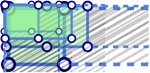
(b) Slim double

(c) Fat double

(d) Degree-4

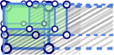
(e) Degree-6

Figure 11: Corner faces for the proof of Fig. 11.

[$\star$]The URFE problem is cubic-time solvable for a plane graph $G$ and it is linear-time solvable if all internal faces of $G$ have maximum degree $6$.

Proof.

If the input is not biconnected, then we can determine that the instance is negative in linear time [DBLP:journals/siamcomp/Tarjan72]. Hence, in the following, we assume that the input is biconnected, which implies that any face is bounded by a cycle.

In order to solve the URFE problem in polynomial time, we guess all the possible rectangular grid drawings of the outer face $f_{o}$. For each of them we invoke Sect. 4.1. We have that, the required drawings of $f_{o}$ are in one-to-one correspondence with the possible choices of two vertices that become consecutive corners of the drawing. This corresponds to $O(n^{2})$ choices. For each choice the algorithm Rectangular-holes Algorithm finds a unit-length grid rectangular drawing in $O(n)$ time, if it exists.

Assume now that all internal faces have maximum degree $6$. Our strategy is to efficiently determine the drawing of the outer face of the input graph $G$ and then to invoke Sect. 4.1 to conclude the proof.

Note that, if $G$ is a $4$-cycle or a $6$-cycle, then the instance is trivially positive. We henceforth assume this is not the case. We have also the following simple cases. A double corner face is a degree-$4$ face with three edges incident to the outer face $f_{o}$ (see Fig. 11(a) for an example). A slim double corner face is a degree-$6$ face with five edges incident to $f_{o}$ (see Fig. 11(b) for an example). A fat double corner face is a degree-$6$ face with four edges incident to $f_{o}$ (see Fig. 11(c)). Consider the cases were $G$ has at least one double corner face, or at least one slim double corner face, or at lost one fat double corner face. In all these cases, since each of the mentioned faces must provide two consecutive $270^{\circ}$ angles incident any realization of $f_{0}$ as a rectangle, the drawing of the outer face is prescribed, and hence Rectangular-holes Algorithm can be invoked.

Suppose now that none of the aforementioned cases holds. A corner face is a degree-$4$ face (resp. degree-6 face) that has two edges (resp. three edges) incident to the outer face $f_{o}$ (see Figs. 11(d) and 11(e), respectively). Observe that, in this setting, a face is incident to a corner of a rectangular drawing of $f_{o}$ if and only if it is a corner face. Hence, since each corner face must provide one $270^{\circ}$ angle incident to any realization of $f_{0}$ as a rectangle, then there must be exactly four corner faces in order for a rectangular drawing of the input instance to exist. Otherwise, the input instance is negative. The four corner faces can be trivially found in $O(n)$ time. They determine a constant number of possible drawings of the outer face as follows. If a corner face has degree-$4$, then its degree-$2$ vertex must be a corner of the drawing of the external face. If a corner face has instead degree-$6$, then one of its two degree-$2$ vertices must be a corner of the drawing of the external face. Hence we have at most $2^{4}=O(1)$ different possible choices for the drawing of the outer face. We solve the URFE problem in this setting by invoking Rectangular-holes Algorithm with each choice as the prescribed drawing of the outer face of $G$.     ∎

To solve the problem in cubic time, we examine the quadratically-many drawings of the outer face $f_{o}$, and invoke Sect. 4.1 for each of them.

Assume now that all internal faces have maximum degree $6$. We efficiently determine $O(1)$ possible rectangular drawings of $f_{o}$ and then invoke Sect. 4.1 for each of them. If $G$ is a $4$-cycle or a $6$-cycle, then the instance is trivially positive. Refer to Fig. 11. A double corner face is a degree-$4$ face with three edges incident to $f_{o}$. A slim double corner face is a degree-$6$ face with five edges incident to $f_{o}$. A fat double corner face is a degree-$6$ face with four edges incident to $f_{o}$. Note that each of such faces must provide two consecutive $270^{\circ}$ angles incident to $f_{0}$. Hence, if $G$ has at least one of the above faces, the drawing of $f_{o}$ is prescribed, and hence Rectangular-holes Algorithm can be invoked.

Suppose now that none of the above cases holds. A corner face is a degree-$4$ (degree-6) face that has two (resp. three) edges incident to $f_{o}$. Each corner face provides a $270^{\circ}$ angle incident to any realization of $f_{0}$ as a rectangle. Hence, there must be exactly four corner faces in order for $G$ to be a positive instance. These faces can be computed in linear time, and determine $O(1)$ possible drawings of the outer face on which we invoke Rectangular-holes Algorithm.

By showing that any planar embedding has a unique candidate outer face supporting a unit-length rectangular drawing, we get the following.

[$\star$] The URFE problem is cubic-time solvable for a planar embedded graph $G$, and it is linear-time solvable if all but at most one face of $G$ have maximum degree $6$.

Proof.

Observe that, given two rectangles $R_{1}$ and $R_{2}$, a necessary condition for drawing $R_{2}$ inside $R_{1}$ is that the perimeter of $R_{2}$ is smaller than the perimeter of $R_{1}$. Hence, given a connected planar embedded graph $G$, we first compute the faces of $G$ with the maximum number of edges in linear time. Suppose that there exists exactly one face $f_{o}$ with the maximum number of edges. We invoke Fig. 11 for checking in cubic time (linear, if all the faces different from $f_{o}$ have degree $6$) if the plane graph consisting of $G$ with the prescribed outer face $f_{o}$ is a positive or negative instance of URFE. Suppose now that there exists more than one face with the maximum number of edges. If $G$ is just an even-length simple cycle, then we conclude that $G$ is a positive instance of URFE. Otherwise, we conclude the opposite.     ∎

Variable Embedding.

Now, we turn our attention to instances with a variable embedding. We start by providing some relevant properties of the graphs that admit a rectangular (not necessarily unit-length or grid) drawing. Let $G$ be one such graph. To avoid degenerate cases, in what follows, we assume that $G$ is not a cycle (cfr. Property 1). Let $\Gamma$ be a rectangular drawing of $G$ and let $\Gamma_{o}$ be the rectangle delimiting the outer face of $\Gamma$. Refer to Fig. 12. Consider the plane graph $G_{\Gamma}$ corresponding to $\Gamma$. Since $\Gamma$ is convex, then $G_{\Gamma}$ is a subdivision of an internally triconnected plane graph [DBLP:conf/compgeom/AngeliniLFLPR15, Theorem 1]. That is, every separation pair $\{u,v\}$ of $G_{\Gamma}$ is such that $u$ and $v$ are incident to the outer face and each connected component of $G_{\Gamma}\setminus\{u,v\}$ contains a vertex incident to the outer face.

5.1 Properties of rectangular drawings

Consider a separation pair $\{u,v\}$ of $G$. In the following, we provide several useful properties related to $\{u,v\}$.

Property 2.

If at least one of $u$ and $v$ is not in $\Gamma_{o}$, then there exist exactly two components of $G$ with respect to $\{u,v\}$, one of which is a simple path. Also, the vertices of such a path are drawn on a straight line. See, e.g., the vertices $x_{1}$ and $y_{1}$ in Fig. 13.

Proof.

The first part of the statement is a consequence of the fact that $G$ is a subdivision of an internally-triconnected plane graph. The second part, instead, follows immediately from the fact that $\Gamma$ is rectangular.     ∎

Property 3.

If both $u$ and $v$ are in $\Gamma_{o}$, then there exist either two or three components of $G$ with respect to $\{u,v\}$.

Proof.

The statement follows from the fact that, since $u$ and $v$ are in $\Gamma_{o}$ and since $\Gamma_{o}$ is drawn as a rectangle, their degree is at most $3$.     ∎

Property 4.

If both $u$ and $v$ are in $\Gamma_{o}$ and $G$ has three components $G_{1}$, $G_{2}$, and $G_{3}$ with respect to $\{u,v\}$, then there is exactly one component, say $G_{2}$, such that $G_{2}\setminus\{u,v\}$ does not contain vertices in $\Gamma_{o}$. Also, $G_{2}$ is a simple path whose vertices are drawn on a straight line. Further $u$ and $v$ are drawn on opposite sides of $\Gamma_{o}$. Furthermore, we have that both $u$ and $v$ have degree $1$ in both $G_{1}$ and $G_{3}$. See, e.g., the vertices $x_{2}$ and $y_{2}$ in Fig. 13.

Proof.

The component $G_{2}$ must be a simple path, since $G$ is a subdivision of an internally-triconnected plane graph. Also, the vertices of such a path must be drawn either along a horizontal or a vertical line, as otherwise $\Gamma$ would not be rectangular. Finally, since $u$ and $v$ are incident to the outer face and since they both have degree $1$ in $G_{2}$, we have that both $u$ and $v$ have degree $1$ in both $G_{1}$ and $G_{3}$.     ∎

Property 5.

There exist no two separation pairs $\{u_{1},v_{1}\}$ and $\{u_{2},v_{2}\}$ of $G$ such that $u_{1}$ and $v_{1}$ lie on opposite sides of $\Gamma_{o}$, $u_{2}$ and $v_{2}$ lie on the opposite side of $\Gamma_{o}$, and $u_{1}$ and $u_{2}$ lie on perpendicular sides of $\Gamma_{o}$.

Proof.

Suppose for a contradiction that there exist two separation pairs $\{u_{1},v_{1}\}$ and $\{u_{2},v_{2}\}$ of $G$ with the properties in the statement. There must exist an internal face $f_{1}$ of $\Gamma$ incident to $u_{1}$ and to $v_{1}$, and an internal face $f_{2}$ of $\Gamma$ incident to $u_{2}$ and to $v_{2}$. However, since $\Gamma$ is rectangular, this is possible only if $f_{1}=f_{2}$, which however contradicts the assumption that $G$ is not a cycle.     ∎

Property 6.

If both $u$ and $v$ are in $\Gamma_{o}$ and $G$ has two components $G_{1}$ and $G_{2}$ with respect to $\{u,v\}$ such that (i) both $G_{1}$ and $G_{2}$ are not simple paths in $G$, and (ii) both $u$ and $v$ have degree $2$ in $G_{1}$, then $u$ and $v$ are drawn on opposite sides of $\Gamma_{o}$ and $G_{1}$ contains a path $P_{1}$ between $u$ and $v$, whose vertices are on a straight line, that is incident to an internal face of $\Gamma$. See, e.g., the vertices $x_{4}$ and $y_{4}$ in Fig. 13.

Proof.

Note that, both $u$ and $v$ are each incident to an internal edge that belongs to $G_{1}$ (possibly the edge $(u,v)$) and each such edge must be incident to the same internal face $f$ of $\Gamma$. Since $f$ is rectangular, the vertices of the subpath $P_{1}$ of $f$ connecting $u$ and $v$ and passing through these edges must be drawn along a straight line. To complete the proof, we observe that this implies that $u$ and $v$ must be drawn on opposite sides of $\Gamma_{o}$.     ∎

The next properties follows from the fact that $\Gamma$ is rectangular.

Property 7.

Suppose that $G$ has two components $G_{1}$ and $G_{2}$ with respect to $\{u,v\}$. If $u$ and $v$ are on the same side of $\Gamma_{o}$, then exactly one of $G_{1}$ and $G_{2}$ is a path whose vertices lie in $\Gamma_{o}$ on a straight line. See, e.g., the vertices $x_{5}$ and $y_{5}$ in Fig. 13.

Property 8.

Suppose that $G$ has two components $G_{1}$ and $G_{2}$ with respect to $\{u,v\}$. If $u$ and $v$ are incident to perpendicular sides of $\Gamma_{o}$, then exactly one of $G_{1}$ and $G_{2}$, say $G_{1}$, is a simple path. Moreover, $G_{1}$ is drawn in $\Gamma$ as an orthogonal polygonal line with a single bend. See, e.g., the vertices $x_{6}$ and $y_{6}$ in Fig. 13.

Property 9.

Suppose that $G$ has two components $G_{1}$ and $G_{2}$ with respect to $\{u,v\}$. If $u$ and $v$ are on opposite sides of $\Gamma_{o}$, then for at least one of $G_{1}$ and $G_{2}$, say $G_{1}$, $u$ and $v$ have degree $1$ in $G_{1}$. See, e.g., the vertices $x_{7}$ and $y_{7}$ in Fig. 13.

A caterpillar is a tree such that removing its leaves results in a path, called spine . The pruned SPQR-tree of a biconnected planar graph $G$, denoted by $T^{*}$, is the tree obtained from the SPQR-tree $T$ of $G$, after removing the $Q$-nodes of $T$.

Figure 12: A rectangular unit-length grid drawing of a planar graph and its pruned SPQR-tree $T^{*}$. $S$-, $P$-, and $R$-nodes are circles, rhombuses and squares, respectively. The subgraphs corresponding to $S$-nodes that are leaves of $T^{*}$ are thick.

[$\star$] Let $G$ be a graph that admits a rectangular drawing. Then the pruned SPQR-tree $T^{*}$ of $G$ is a caterpillar with the following properties: (i) All its leaves are $S$-nodes; (ii) its spine contains no two adjacent $R$-nodes; (iii) its spine contains no two adjacent nodes $\mu$ and $\nu$, such that $\mu$ is a $P$-node and $\nu$ is an $R$-node; (iv) each $P$-node $\mu$ has exactly $3$ neighbors; and (v) the skeleton of each $S$-node of the spine of $T^{*}$ contains two chains of virtual edges corresponding to $Q$-nodes, separated by two virtual edges each corresponding to either a $P$- or an $R$-node.

Proof.

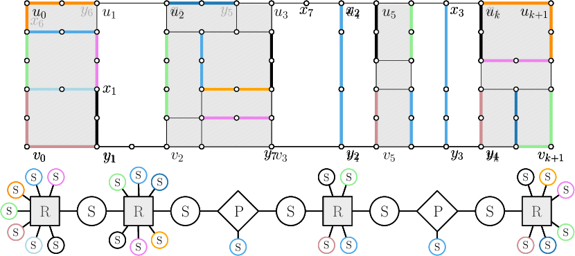
Figure 13: A rectangular unit-length grid drawing of a planar graph and its pruned SPQR-tree $T^{*}$. $S$-, $P$-, and $R$-nodes are circles, rhombuses and squares, respectively. The subgraphs corresponding to $S$-nodes that are leaves of $T^{*}$ are thick.

In the following, we assume that $G$ is not a cycle, as otherwise the statement trivially holds. Let $\Gamma$ be a rectangular drawing of $G$, and let $\Gamma_{o}$ be the drawing of the outer face of $\Gamma$. Refer to Fig. 13.

Suppose, for a contradiction, that there exist two adjacent $R$-node $\mu$ and $\nu$ in the spine of $T^{*}$. Let $\{u,v\}$ be the separation pair shared by their skeletons, and let $e_{\mu,\nu}$ and $e_{\nu,\mu}$ be the the virtual edges in $\operatorname{sk}(\nu)$ and in $\operatorname{sk}(\mu)$ corresponding to $\mu$ and to $\nu$, respectively. By Property 2, both $u$ and $v$ must lie in $\Gamma_{o}$. By Property 8, $u$ and $v$ must lie on opposite sides of $\Gamma_{o}$. Therefore, by Property 9, for at least one of $\exp{e_{\mu,\nu}}$ and $\exp{e_{\nu,\mu}}$ we have that $u$ and $v$ have degree $1$, which implies that either $\mu$ or $\nu$ is an $S$-node. Therefore, we get a contradiction. This proves Condition (ii) of the statement. By Property 4, the neighbors of a $P$-node are either S- or Q-nodes. This proves Condition (iii). By Properties 2 and 3, if $T$ has a $P$-node $\mu$, then $\mu$ has three neighbors. This proves Condition (iv).

Next, we show that $T^{*}$ is a caterpillar, and that it satisfies Conditions (i) and (v) of the statement.

Suppose first that there exist no separation pair $\{u,v\}$ of $G$ such that $u$ and $v$ are on opposite sides of $\Gamma_{o}$. In this case, by Property 4, $T^{*}$ contains no $P$-nodes. Also, all the separation pairs of $G$ have either an internal vertex, or vertices on perpendicular sides of $\Gamma_{o}$, or vertices on the same side of $\Gamma_{o}$. In the first case, by Property 2, in the second case, by Property 8, and in the third case, by Property 7, we have that (i) for each of these separation pairs, there exist exactly two components of $G$ with respect to it and that (ii) for each of these separation pairs, exactly one of the components of $G$ with respect to it corresponds to an $S$-node, which is a simple path. It follows that there exist no two $R$-nodes in $T$. Therefore, $T^{*}$ is a star whose leaves are $S$-nodes and whose central vertex is an $R$-node.

Suppose now that there exists a separation pair $\{u,v\}$ of $G$ such that $u$ and $v$ are on opposite sides of $\Gamma_{o}$. By Property 5, any other separation pair $\{u^{\prime},v^{\prime}\}$ different from $\{u,v\}$ where $u^{\prime}$ and $v^{\prime}$ are on opposite sides of $\Gamma_{o}$ is such that either $u$ and $u^{\prime}$ are on the same side of $\Gamma_{o}$ or $u$ and $v^{\prime}$ are on the same side of $\Gamma_{o}$. Therefore, after a possible rotation by a multiple of $90^{\circ}$, in the following we will assume that $u$ lies on the top side of $\Gamma_{o}$ and $v$ lies on the bottom side of $\Gamma_{o}$. Let $S=[\{u_{1},v_{1}\},\{u_{2},v_{2}\},\dots,\{u_{k},v_{k}\}]$ be the separation pairs of $G$ such that both $u_{i}$ and $v_{i}$ lie on opposite sides of $\Gamma_{o}$, have degree $3$, and share the same $x$-coordinate, for $i=1,\dots,k$, sorted in increasing order of their $x$-coordinate. The next claim shows that $k\geq 1$.

Claim.

Unless $G$ is a cycle, if there exists a separation pair $\{u,v\}$ of $G$ such that $u$ and $v$ are on opposite sides of $\Gamma_{o}$, then there exists at least a separation pair $\{u^{\prime},v^{\prime}\}$ such that $u^{\prime}$ and $v^{\prime}$ are on opposite sides of $\Gamma_{o}$, both $u^{\prime}$ and $v^{\prime}$ have degree $3$ in $G$, and $u^{\prime}$ and $v^{\prime}$ share the same $x$-coordinate in $\Gamma$.

Proof. Consider a separation pair $\{u^{\prime},v^{\prime}\}$ such that $u^{\prime}$ and $v^{\prime}$ are on opposite sides of $\Gamma_{o}$, possibly $u^{\prime}=u$ and $v^{\prime}=v$.

Suppose first that at least one of $u^{\prime}$ and $v^{\prime}$, say $v^{\prime}$, has degree-$3$. We show that there exists a vertex $u^{\prime\prime}$ lying along the top side of $\Gamma_{o}$, possibly $u^{\prime\prime}=u^{\prime}$, such that $\{u^{\prime\prime},v^{\prime}\}$ is a separation pair, $u^{\prime\prime}$ has degree $3$, and $u^{\prime\prime}$ and $v^{\prime}$ have the same $x$-coordinate. Note that, since $v^{\prime}$ has degree $3$ and it is incident to the bottom side of $\Gamma_{o}$, two of its neighbors lie along the bottom side of $\Gamma_{o}$. Therefore, the third neighbor of $v^{\prime}$, must either be a vertex $u^{*}$ incident to the top side of $\Gamma_{o}$ (possibly $u^{*}=u^{\prime}$) or an internal vertex $i_{v}$ lying vertically above $v^{\prime}$. In the former case, since $\Gamma$ is rectangular, we have that $u^{*}$ has degree $3$ and lies vertically above $v^{\prime}$ in $\Gamma$ (which implies that $u^{*}$ and $v^{\prime}$ have the same $x$-coordinate). Thus, setting $u^{\prime\prime}=u^{*}$ yields the desired separation pair. In the latter case, since $\{u^{\prime},v^{\prime}\}$ is a separation pair, there exists an internal face $f$ shared by $u^{\prime}$, $v^{\prime}$, and $i_{v}$. Let $u^{\prime\prime}$ be the first vertex of the top side of $\Gamma_{o}$ that is encountered when traversing the boundary of $f$ starting at $v^{\prime}$ and passing through $i_{v}$. Consider the subpath of $f$ between $v^{\prime}$ and $u^{\prime\prime}$ that contains $i_{v}$. Since $i_{v}$ lies vertically above $v^{\prime}$ in $\Gamma$, and since $\Gamma$ is rectangular, this path must be drawn as a straight-line segment between $v^{\prime}$ and $u^{\prime\prime}$, which implies that $u^{\prime\prime}$ has degree $3$ and has the same $x$-coordinate as $v^{\prime}$. Therefore, since both $u^{\prime\prime}$ and $v^{\prime}$ belong to $f$ and lie on opposite sides of $\Gamma_{o}$, they form the sought separation pair.

Suppose next that both $u^{\prime}$ and $v^{\prime}$ have degree-$2$. Consider the internal face $f$ of $\Gamma$ shared by $u^{\prime}$ and $v^{\prime}$. We show that there exists a separation pair that satisfies the properties of the statement whose vertices are incident to $f$. If $f$ contains no degree-$3$ vertex incident to the top side of $\Gamma_{o}$ and no degree-$3$ vertex incident to the bottom side of $\Gamma_{o}$, then both the paths of $G$ that form the top and the bottom side of $\Gamma_{o}$ belong to $f$, we have that $G$ is a cycle, which contradicts the assumption in the statement. If $f$ contains a degree-$3$ vertex incident to the top side of $\Gamma_{o}$ and no degree-$3$ vertex incident to the bottom side of $\Gamma_{o}$ (the opposite case being symmetric), then the vertices lying at the bottom-left and bottom-right corner of $\Gamma_{o}$ form a separation pair, which contradicts Property 5. Therefore, there must exist a separation pair $\{u^{\prime\prime},v^{\prime\prime}\}$ incident to $f$ such that $u^{\prime\prime}$ is incident to the top side of $\Gamma_{o}$ and has degree $3$ in $G$, and $v^{\prime\prime}$ is incident to the bottom side of $\Gamma_{o}$ and has degree $3$ in $G$. If $u^{\prime\prime}$ and $v^{\prime\prime}$ have the same $x$-coordinate, then they form the sought separation pair. Otherwise, as discussed in the previous case, there exists a vertex $u^{\prime\prime\prime}$ (and a vertex $v^{\prime\prime\prime}$) of degree $3$ such that $\{u^{\prime\prime},v^{\prime\prime\prime}\}$ (and $\{u^{\prime\prime\prime},v^{\prime\prime}\}$)) is a separation pair, and $u^{\prime\prime}$ and $v^{\prime\prime\prime}$ (and $u^{\prime\prime\prime}$ and $v^{\prime\prime}$) share the same $x$-coordinate.  $\blacksquare$

Note that, by Properties 4 and 6, for $i=1,\dots,k$, there exists a path $P_{i}$ between $u_{i}$ and $v_{i}$ drawn along a vertical line that is incident to an internal face in $\Gamma$.

We set $L=\{u_{0},v_{0}\}\circ S\circ\{u_{k+1},v_{k+1}\}$, where $u_{0}$ is the vertex lying on the top-left corner of $\Gamma_{o}$, $v_{0}$ is the vertex lying on the bottom-left corner of $\Gamma_{o}$, $u_{k+1}$ is the vertex lying on the top-right corner of $\Gamma_{o}$, and $v_{k+1}$ is the vertex lying on the bottom-right corner of $\Gamma_{o}$; where $\circ$ denotes the concatenation operator. Consider any two consecutive pairs $\{u_{i},v_{i}\}$ and $\{u_{i+1},v_{i+1}\}$, for $i=0,\dots,k$. By the previous observation, we can define a cycle $C_{i}$ in $G$ that contains $u_{i}$, $u_{i+1}$, $v_{i+1}$, and $v_{i}$, that contains $P_{i}$ and $P_{i+1}$, and that is drawn as a rectangle in $\Gamma$. Clearly, any two cycles $C_{i}$ and $C_{i+1}$ share the path $P_{i+1}$. We denote by $G_{i}$ the subgraph of $G$ induced by the vertices in the interior and along the boundary of $C_{i}$.

We will construct $T^{*}$ iteratively starting from the empty tree as follows. At each point $T^{*}$ will be a caterpillar whose spine does not have a $P$-node as an end-point. Also, a leaf of $T^{*}$ will be denoted as active and will be used in the subsequent iteration as an attachment endpoint to extend $T^{*}$.

If $G_{0}=C_{0}$, we introduce an $S$-node $\mu_{0}$ in $T^{*}$. In particular, one virtual edges of $\operatorname{sk}(\mu_{0})$ is the edge $(u_{1},v_{1})$, and the other virtual edges correspond to the real edges of $C_{0}$ that are incident to the outer face. Otherwise, $G_{0}\neq C_{0}$. Consider a separation pair $\{u,v\}$ of $G_{0}$. By Sect. 5.1 and since $\{u_{1},v_{1}\}$ is the first pair in $S$, we have that $u$ and $v$ do not lie on opposite sides of $\Gamma$. Therefore, by Properties 2, 7 and 8, one of the two components of $G_{0}$ with respect to $\{u,v\}$ is a simple path. Thus, $G_{0}$ is the subdivision of a triconnected planar graph. Hence, we introduce an $R$-node $\mu_{0}$ in $T^{*}$ whose skeleton is obtained by replacing each simple path in $G_{0}$ with a virtual edge. We add an $S$-node for each of such virtual edges. Also, we introduce in $\operatorname{sk}(\mu_{0})$ the virtual edge $(u_{1},v_{1})$. In both cases (i.e., $G_{0}=C_{0}$ and $G_{0}\neq C_{0}$), $\mu_{0}$ is the active endpoint of $T^{*}$.

Next, for $i=1,\dots,k$, we consider the separation pair $\{u_{i},v_{i}\}$. Denote by $\xi$ the active endpoint of the spine (right before considering the current index $i$). Two cases are possible: Either $\xi$ is an $S$-node or it is an $R$-node. Suppose that $G_{i}=C_{i}$. If $\xi$ is an $S$-node, then we introduce a $P$-node $\mu_{i,1}$ in $T^{*}$ adjacent to $\xi$, and two $S$-nodes $\mu_{i,2}$ and $\mu_{i,3}$ adjacent to $\mu_{i,1}$. In particular, the skeleton of $\mu_{i,1}$ is a bundle of three parallel edges $(u_{i},v_{i})$. The skeleton of $\mu_{i,2}$ is a cycle containing one virtual edge for each edge of the path $P_{i}$ plus a virtual edge $(u_{i},v_{i})$. The skeleton of $\mu_{i,3}$ is a cycle consisting of a virtual edge $(u_{i},v_{i})$, followed one virtual edge for each horizontal edge in the top side of $C_{i}$, followed by one virtual edge $(u_{i+1},v_{i+1})$, followed by one virtual edge for each horizontal edge in the bottom side of $C_{i}$. Finally, we set $\mu_{1,3}$ as the active node of $T^{*}$. If $\xi$ is an $R$-node, then we introduce an $S$-node $\mu_{i}$ in $T^{*}$ adjacent to $\xi$ whose skeleton is a cycle consisting of a virtual edge $(u_{i},v_{i})$, followed by one virtual edge for each horizontal edge in the top side of $C_{i}$, followed by a path $P^{*}$ of virtual edges defined below, followed by one virtual edge for each horizontal edge in the bottom side of $C_{i}$. If $i<k$, then the path $P^{*}$ consists of the single virtual edge $(u_{i+1},v_{i+1})$; otherwise, if $i=k$, then the path $P^{*}$ contains a virtual edge for each real edge incident to the right side of $\Gamma_{o}$ (i.e., for each edge of the right side of $C_{k}$). Finally, we set $\mu_{i}$ as the active endpoint of $T^{*}$, unless $i=k$. In particular, note that, the skeleton of $\mu_{i}$ satisfies Condition (v) of the statement. Suppose now that $G_{i}\neq C_{i}$. With the same motivation as for $G_{0}$, we introduce an $R$-node $\mu_{i}$ in $T^{*}$ adjacent to $\xi$ whose skeleton is obtained by replacing each simple path in $G_{i}$ with a virtual edge. We add an $S$-node for each of such virtual edges. Also, we introduce in $\operatorname{sk}(\mu_{i})$ the virtual edges $(u_{i},v_{i})$, and the edge $(u_{i+1},v_{i+1})$ unless $i=k$. Finally, we set $\mu_{i}$ as the active endpoint of $T^{*}$, unless $i=k$. This concludes the proof that $T^{*}$ is a caterpillar.

Finally, observe that, by construction, each leaf of $T^{*}$ is an $S$-node, which proves Condition (i).     ∎

Let $\Gamma$ be a rectangular drawing of $G$ and let $\Gamma_{o}$ be the rectangle bounding the outer face of $\Gamma$. By inspecting $\Gamma$ “from left to right”, we argue about the structure of $T^{*}$, which ultimately leads to prove the statement of the lemma; refer to Fig. 12. At each point of the inspection, $T^{*}$ will be a caterpillar whose spine does not have a $P$-node as an end-point. Also, a leaf will be denoted as active and will be used as an attachment endpoint to extend $T^{*}$.

Let $S=[\{u_{1},v_{1}\},\{u_{2},v_{2}\},\dots,\{u_{k},v_{k}\}]$ be the separation pairs of $G$ such that both $u_{i}$ and $v_{i}$ lie on opposite sides of $\Gamma_{o}$, have degree $3$, and share the same $x$-coordinate, for $i=1,\dots,k$, sorted in increasing order of their $x$-coordinate. In Sect. 5.1, we provide properties of rectangular drawings that show that these pairs are the only ones that correspond to poles of $P$- and $R$-nodes of $T^{*}$. We set $L=\{u_{0},v_{0}\}\circ S\circ\{u_{k+1},v_{k+1}\}$, where $u_{0}$, $u_{k+1}$, $v_{k+1}$, and $v_{0}$ are the vertices on the top-left, top-right, bottom-right, and bottom-left corner of $\Gamma_{o}$.

Consider any two consecutive pairs $\{u_{i},v_{i}\}$ and $\{u_{i+1},v_{i+1}\}$, for $i=0,\dots,k$. We can define a cycle $C_{i}$ in $G$ that contains $u_{i}$, $u_{i+1}$, $v_{i+1}$, and $v_{i}$, and that is drawn as a rectangle in $\Gamma$. Moreover, any two cycles $C_{i}$ and $C_{i+1}$ share a path $P_{i+1}$ that is drawn as a straight-line segment in $\Gamma$. We denote by $G_{i}$ the subgraph of $G$ induced by the vertices in the interior and along the boundary of $C_{i}$.

We skip the discussion for the consecutive pairs $\{u_{0},v_{0}\}$ and $\{u_{1},v_{1}\}$. For $i=1,\dots,k$, consider the separation pair $\{u_{i},v_{i}\}$. Let $\xi$ be the active endpoint of the spine. In the following, we denote by $\operatorname{sk}(\mu)$ the skeleton of a node $\mu$ of $T^{*}$. Two cases are possible: $\xi$ is either an $S$- or an $R$-node.

Suppose that $G_{i}=C_{i}$. If $\xi$ is an $S$-node, then we introduce a $P$-node $\mu_{i,1}$ in $T^{*}$ adjacent to $\xi$ and to two new $S$-nodes $\mu_{i,2}$ and $\mu_{i,3}$. We have that $\operatorname{sk}(\mu_{i,1})$ is a bundle of three parallel edges $(u_{i},v_{i})$, $\operatorname{sk}(\mu_{i,2})$ is a cycle containing one virtual edge for each edge of the path $P_{i}$ plus a virtual edge $(u_{i},v_{i})$, and $\operatorname{sk}(\mu_{i,3})$ is a cycle consisting of a virtual edge $(u_{i},v_{i})$, followed by one virtual edge for each horizontal edge in the top side of $C_{i}$, followed by one virtual edge $(u_{i+1},v_{i+1})$, followed by one virtual edge for each horizontal edge in the bottom side of $C_{i}$. We set $S$-node $\mu_{1,3}$ as the active node of $T^{*}$. If $\xi$ is an $R$-node, then we introduce an $S$-node $\mu_{i}$ in $T^{*}$ adjacent to $\xi$ whose skeleton is a cycle consisting of a virtual edge $(u_{i},v_{i})$, followed by one virtual edge for each horizontal edge in the top side of $C_{i}$, followed by a path $P^{*}$ of virtual edges defined below, followed by one virtual edge for each horizontal edge in the bottom side of $C_{i}$. If $i<k$, then $P^{*}$ consists of the single virtual edge $(u_{i+1},v_{i+1})$; otherwise, if $i=k$, then $P^{*}$ contains a virtual edge for each real edge incident to the right side of $\Gamma_{o}$. We set the $S$-node $\mu_{i}$ as the active endpoint of $T^{*}$, unless $i=k$.

Suppose now that $G_{i}\neq C_{i}$. In this case, $G_{i}$ is the subdivision of a triconnected planar graph. We introduce an $R$-node $\mu_{i}$ in $T^{*}$ adjacent to $\xi$ and to the $S$-nodes corresponding to the components of $G_{i}$, with respect to its split pairs, that are simple paths. We add to $\operatorname{sk}(\mu_{i})$ a virtual edge for each of such paths, as well as $(u_{i},v_{i})$ and $(u_{i+1},v_{i+1})$, unless $i=k$. We set the $R$-node $\mu_{i}$ as the active endpoint of $T^{*}$, unless $i=k$.

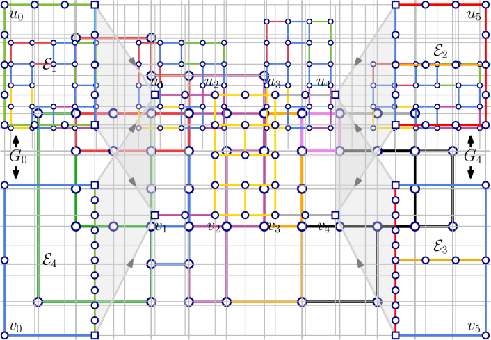
Figure 14: Four plane embeddings of a graph $G$ that support a rectangular drawing of $G$, obtained by selecting one of the plane embeddings ${\cal E}_{1}$ and ${\cal E}_{4}$ of the subgraph $G_{0}$ of $G$ and one of the the plane embeddings ${\cal E}_{2}$ and ${\cal E}_{3}$ of the subgraph $G_{4}$ of $G$. Only the embeddings ${\cal E}_{1}$ and ${\cal E}_{2}$ support a unit-length rectangular drawing.

Consider a graph $G$ that satisfies the conditions of Fig. 12. If the spine of the pruned SPQR-tree of $G$ contains at least two nodes or at least one $P$-node, we say that $G$ is flat; otherwise, $G$ is the subdivision of a triconnected planar graph. Exploiting Fig. 12, we can prove the following; refer to Fig. 14.

[$\star$] Let $G$ be an $n$-vertex graph. The following hold:

• All the unit-length rectangular drawings of $G$, if any, have the same plane embedding $\cal E$ (up to a reflection), which can be computed in $O(n)$ time.

• If $G$ is flat, all the rectangular drawings of $G$, if any, have at most four possible plane embeddings (up to a reflection), which can be computed in $O(n)$ time.

Proof.

We prove the first part of the statement.

Suppose that $G$ has a unit-length rectangular drawings $\Gamma$. By Fig. 12, the pruned SPQR-tree $T^{*}$ of $G$ is a caterpillar. Since all the nodes of $T^{*}$ that are not in the spine are $S$-nodes, all the planar embeddings of $G$ are obtained by embedding the skeletons of the $P$- and $R$-nodes of the spine of $T^{*}$.

We arbitrarily select a normal orientation $T^{*}$ such that its spine is a directed path, and visit the spine $\mu_{1},\dots,\mu_{k}$ of $T^{*}$ according to such an orientation. Note that, neither $\mu_{1}$ nor $\mu_{k}$ can be an $S$-node. We construct the plane embedding $\cal E$ of $G$ and select its outer face $f_{o}$ as follows. All the choices we perform are obliged and are a consequence of Fig. 12 and of the properties in Sect. 5.1.

Suppose that $\mu_{1}$ is a $P$-node. By Property 4, we have that either (i) exactly one neighbor $\nu$ of $\mu_{1}$ is a $Q$-node, or (ii) exactly one neighbor $\nu$ of $\mu_{1}$ is an $S$-node corresponding to a simple path in $G$, or (iii) at least two neighbors of $\mu_{1}$ are $S$-nodes corresponding to a simple path in $G$. In all cases, the poles of $\mu$ are incident to $f_{o}$. In cases (i) and (ii), the virtual edge of $\operatorname{sk}(\mu_{1})$ corresponding to $\nu$ must lie in between the other two virtual edges. In case (iii), since $\Gamma$ is rectangular, one of the simple paths corresponding to the neighbors of $\mu$ must be shorter than the others. The corresponding virtual edge must lie in between the other virtual edges in the embedding of $\operatorname{sk}(\mu_{1})$. Two cases are possible: Either $\mu_{1}$ is the unique node of the spine of $T^{*}$ or not. In the former case, the virtual edges corresponding to the remaining two neighbors of $\mu_{1}$ in $T^{*}$ can be ordered arbitrarily. Note that, this yields exactly two planar embeddings of $G$ that are one the reflection of the other. Otherwise, we set the virtual edge corresponding to $\mu_{2}$ at the rightmost virtual edge in the embedding of $\operatorname{sk}(\mu_{1})$.

Suppose that $\mu_{1}$ is an $R$-node. Two cases are possible: Either $\mu_{1}$ is the unique node of the spine of $T^{*}$ or not. In the former case, $G$ is the subdivision of a triconnected planar graph. Hence, it has a unique planar embedding $\cal E$. Since in any unit-length rectangular drawing of $G$, the outer face must be bounded by a face of $\cal E$ of maximum size and since no internal face may have the same size of the outer face, we can determine in $O(n)$ time whether $\cal E$ does not support a rectangular drawing or whether a candidate outer face of $\cal E$ exists. This determines a unique candidate plane embedding of $G$. In the latter case, consider the virtual edge $e_{2}$ corresponding to $\mu_{2}$ in $\operatorname{sk}(\mu_{1})$. Recall that, since $\mu_{1}$ is a $R$-node, $\operatorname{sk}(\mu_{1})$ admits a unique (up to a flip) planar embedding. In such an embedding, we remove the edge $e_{1}=(u_{1},v_{1})$, and let $\operatorname{sk}^{-}{\mu_{1}}$ be the resulting embedded graph. Note that, by Condition (i), each virtual edge of $\operatorname{sk}^{-}{\mu_{1}}$ corresponds to a simple path in $G$. Let $G^{-}$ be the embedded subgraph of $G$ obtained by replacing each virtual edge of $\operatorname{sk}^{-}{\mu_{1}}$ with the associated path. Let $P$ and $P_{1}$ be the two paths of $G^{-}$ between $u_{1}$ and $v_{1}$ that share the same face of $G^{-}$ (note that, they stem from the face of $\operatorname{sk}^{-}{\mu_{1}}$ that used to host the edge $e_{1}$). Since $\Gamma$ is unit-length and rectangular, one of $P$ and $P_{1}$, say $P_{1}$, is shorter than the other. We select the embedding of $\operatorname{sk}(\mu_{1})$ so that the path of $\operatorname{sk}(\mu_{1})$ that corresponds to $P_{1}$ is incident to the right outer face of the embedding of $\operatorname{sk}(\mu_{1})$.

Consider now a node $\mu_{i}$, with $1<i<k$. Let $e_{i-1}$ and let $e_{i}$ be the virtual edges of $\operatorname{sk}(\mu_{i})$ corresponding to $\mu_{i-1}$ and $\mu_{i+1}$. In all cases, the poles of $\mu_{i}$ are incident to $f_{o}$.

Suppose that $\mu_{i}$ is an $S$-node. In this case, there is not embedding choice to perform.

Suppose that $\mu_{i}$ is a $P$-node. Let $\nu$ be the neighbor of $\mu_{i}$ different from $\mu_{i-1}$ and $\mu_{i+1}$. By Property 4, we have that either (i) $\nu$ is a Q-node, or (ii) $\nu$ is an $S$-node corresponding to a simple path in $G$. In both cases, the virtual edge of $\operatorname{sk}(\mu_{i})$ corresponding to $\nu$ lies in between $e_{i-1}$ and $e_{i}$. Also, we let $e_{i-1}$ and $e_{i}$ be the left-most and the right-most virtual edges in the embedding of $\operatorname{sk}(\mu_{i})$, respectively.

Suppose that $\mu_{i}$ is an $R$-node. Recall that, since $\mu_{i}$ is a $R$-node, $\operatorname{sk}(\mu_{i})$ admits a unique (up to a flip) planar embedding. We select the embedding of $\operatorname{sk}(\mu_{i})$ so that $e_{i-1}$ and $e_{i}$ are incident to the left outer face and to the right outer face of such an embedding, respectively.

Finally, consider now the node $\mu_{k}$. The embedding of $\operatorname{sk}(\mu_{k})$ can be selected, based on its type, as described for $\mu_{1}$.

Now, we prove the second part of the statement. First, observe that, since a rectangular drawing of $G$ is convex, the separation pairs corresponding to the poles of $P$- and $R$-nodes must be incident to the outer face of any rectangular drawing of $G$ [DBLP:books/ws/NishizekiR04, DBLP:journals/iandc/BattistaTV01]. Therefore, the embedding choices for the $P$- and $R$-nodes $\mu_{i}$, with $1<i<k$, in an embedding that supports a rectangular drawing are obliged and correspond to the ones described above. Therefore, the only remaining embedding choices occur on $\mu_{1}$ and $\mu_{k}$.

If $k=1$, then the spine of $T^{*}$ contains a single node. If $\mu_{1}=\mu_{k}$ is an $R$-node, then $G$ is not flat and it is the subdivision of a triconnected planar graph and there is nothing to prove. Otherwise, $\mu_{1}=\mu_{k}$ is a $P$-node, and $G$ consists of three parallel simple paths. Therefore, it admits three plane embeddings, up to a reflection.

Otherwise, $k\neq 1$. Consider $\mu_{1}$. If $\mu_{1}$ is an $R$-node, then consider the subgraph $G_{0}$ of $G$ corresponding to it. Namely, let $e_{\mu_{1},\mu_{2}}$ the the virtual edge of $\operatorname{sk}(\mu_{2})$ corresponding to $\mu_{1}$, then $G_{0}=\exp(e_{\mu_{1},\mu_{2}})$. As shown above, $G_{0}$ is the subdivision of a triconnected planar graph. Since it admits a unique planar embedding (up to a flip), since there exists a unique face of such and embedding that contains the poles of $\mu_{1}$, and since these vertices must be incident to the outer face of a plane embedding of $G$ that supports a rectangular drawing of $G$, we have that $G_{0}$ admits only two candidates plane embedding. If $\mu_{1}$ is a $P$-node, then let $\nu_{1}$, $\nu_{2}$, and $\nu_{3}$ be its three neighbors (see Fig. 12) and let $\nu_{3}$ be its neighbor in the spine of $T^{*}$. By Fig. 12, $\nu_{1}$ and $\nu_{2}$ are $S$-nodes whose corresponding subgraph of $G$ is a simple path, whereas the subgraph of $G$ corresponding to $\nu_{3}$ is not a simple path. Note that, because any rectangular drawing is also convex, the embedding $\mathcal{E}_{1}$ of $\operatorname{sk}(\mu_{1})$ induced by any embedding of $G$ that supports a rectangular drawing is such that the virtual edge corresponding to $\nu_{3}$ is incident to the outer face of $\mathcal{E}_{1}$. It follows that the only two possible choices to determine a candidate embedding of $\operatorname{sk}(\mu_{1})$ depend on the fact that the virtual edge corresponding to $\nu_{1}$ is before or after the virtual edge corresponding to $\nu_{2}$. The degrees of freedom of the embeddings of $\operatorname{sk}(\mu_{k})$ are analogous. Hence, if $k\neq 1$ we have four possible plane embeddings of $G$, up to a reflection.     ∎

The next theorem shows that the UR problem is polynomial-time solvable. Surprisingly, the problem seems to be harder for non-flat instances.

[$\star$] Let $G$ be a planar graph. The UR problem is cubic-time solvable for $G$. Also, if $G$ is flat, then the UR problem is linear-time solvable.

Proof.

First, we test whether $G$ satisfies the conditions of Fig. 12, which can clearly be done in $O(n)$ time by computing and visiting $T^{*}$, and reject the instance if this test fails. Then, by Fig. 14, we compute in $O(n)$ time the unique candidate plane embedding $\cal E$ of $G$ that may support a unit-length rectangular drawing of $G$, if any, and reject the instance if such an embedding does not exist. Let $f_{o}$ be the outer face of $\cal E$. If the spine of $T^{*}$ consists of a single $R$-node, then $\cal E$ coincides with the unique planar embedding of $G$, and we test for the existence of such a drawing using Fig. 11 in $O(n^{3})$ time. If $G$ is flat, then we can show that there exists a unique candidate drawing $\Gamma_{o}$ of $f_{o}$. In this case, we use Sect. 4.1 to test in $O(n)$ time for the existence of a unit-length rectangular drawing of $G$ that respects the plane embedding $\cal E$ and such that $f_{o}$ is drawn as the rectangle $\Gamma_{o}$.

Consider the pruned SPQR-tree $T^{*}$ of $G$. If the spine of $T^{*}$ does not consist of a single $R$-node, then two cases are possible: (Case 1) the spine of $T^{*}$ contains a $P$-node or (Case 2) the spine of $T^{*}$ does not contain a $P$-node. In Case 1, let $\mu$ be a $P$-node of the spine of $T^{*}$, and let $u$ and $v$ be the poles of $\mu$. By Property 4, these vertices lie on opposite sides of the outer face $\Gamma_{o}$ of any rectangular drawing $\Gamma$ of $G$ and there exists exactly one component of $G$ with respect to $\{u,v\}$ that is a simple path $P$ whose vertices are drawn on a straight line in $\Gamma$. In Case 2, let $\mu$ be an $R$-node of the spine of $T^{*}$, and let $u$ and $v$ be the poles of $\mu$. Note that, there exists a neighbor $\nu$ of $\mu$ in the spine of $T^{*}$ that is an $S$-node. By Property 6, these vertices lie on opposite sides of the outer face $\Gamma_{o}$ of any rectangular drawing $\Gamma$ and there exists a path $P$ between $u$ and $v$ that belong to the component of $G$ with respect to $\{u,v\}$ that does not correspond to $\nu$; also, the path $P$ is incident to an internal face of $\Gamma$ and its vertices are drawn on a straight line. In both Case 1 and Case 2, let $|P|$ and $|f_{o}|$ denote the length of $P$ and $f_{o}$, respectively. By Property 4, up to a $90^{\circ}$ rotation of $\Gamma$, the value $|P|$ must correspond to the height of $\Gamma$, whereas $(|f_{o}|-2|P|)/2$ must correspond to the width of $\Gamma$. Note that, if the latter value is less or equal than zero then $G$ does not admit a unit-length rectangular drawing, in which case we reject the instance. Let $r$ (resp. $\ell$) be the length of the subpath of $f_{o}$ between $u$ and $v$ that is encountered by traversing $f_{o}$ clockwise (resp. counter-clockwise) starting from $u$. By the above discussion, the drawing of $\Gamma_{o}$ of $f_{o}$ is uniquely defined and this implies a unique choice for the four vertices $u_{\ell}$, $u_{r}$, $v_{r}$, and $v_{\ell}$ in $f_{o}$ that may act as the top-left, top-right, bottom-right, and bottom-left corners of the drawing of a rectangle bounding $f_{o}$, respectively. The vertex $u_{r}$ is the vertex at distance $(r-|P|)/2$ from $u$ that is encountered by traversing $f_{o}$ clockwise starting from $u$. The vertex $v_{r}$ is the vertex at distance $|P|$ from $u_{r}$ that is encountered by traversing $f_{o}$ clockwise starting from $v_{r}$. The vertex $u_{\ell}$ is the vertex at distance $(\ell-|P|)/2$ from $u$ that is encountered by traversing $f_{o}$ counter-clockwise starting from $u$. The vertex $v_{\ell}$ is the vertex at distance $|P|$ from $u_{\ell}$ that is encountered by traversing $f_{o}$ counter-clockwise starting from $v_{\ell}$.     ∎

First, we test whether $G$ satisfies the conditions of Fig. 12, which can clearly be done in $O(n)$ time by computing and visiting $T^{*}$, and reject the instance if this test fails. Then, by Fig. 14, we compute in $O(n)$ time the unique candidate plane embedding $\cal E$ of $G$ that may support a unit-length rectangular drawing of $G$, if any, and reject the instance if such an embedding does not exist. Let $f_{o}$ be the outer face of $\cal E$. If the spine of $T^{*}$ consists of a single $R$-node, then $\cal E$ coincides with the unique planar embedding of $G$, and we test for the existence of such a drawing using Fig. 11 in $O(n^{3})$ time. If $G$ is flat, then we can show that there exists a unique candidate drawing $\Gamma_{o}$ of $f_{o}$. Then, we use Sect. 4.1 to test in $O(n)$ time whether a unit-length rectangular drawing of $G$ exists that respects $\cal E$ and such that $f_{o}$ is drawn as $\Gamma_{o}$.

[$\star$] Let $G$ be an $n$-vertex planar graph. The problem of testing for the existence of a rectangular drawing of $G$ is solvable in $O(n^{2}\log^{3}n)$ time. Also, if $G$ is flat, then this problem is solvable in $O(n\log^{3}n)$ time.

Proof.

First, we test whether $G$ satisfies the conditions of Fig. 12, which can clearly be done in $O(n)$ time by computing and visiting $T^{*}$, and reject the instance if this test fails.

We start by considering the case that $G$ is flat. Due to Fig. 14, only up to four plane embeddings of $G$ are candidates for a rectangular drawing of $G$ that respects them. Also, such embeddings can be computed in $O(n)$ time. For each of them, we test for the existence of a rectangular drawing respecting it by solving a max-flow problem on a linear-size planar network with multiple sources and sinks in $O(n\log^{3}n)$ time [DBLP:journals/siamcomp/BorradaileKMNW17]. Such a network can be defined following Tamassia’s [DBLP:books/ph/BattistaETT99] classic approach to test for the existence of rectilinear drawings of plane graphs. In such a network $\cal N$: (i) Each node of $\cal N$ corresponding to a vertex of $G$ is a source producing $4$ units of flow, each corresponding to a $90^{\circ}$ angle; (ii) Each node of $\cal N$ corresponding to a face $f$ of $G$ is a sink consuming $2|f|-4$ (resp. $2|f|+4$) units of flow if $f$ is an internal face (resp. the outer face) of $G$, where $f$ is the length of $f$: (iii) Each node of $\cal N$ corresponding to a vertex of $G$ has an outgoing arc directed toward the nodes corresponding to its incident faces; (iv) Each arc of $\cal N$ has a lower bound of $1$ unit of flow. The existence of a flow in $\cal N$ from the sources to the sinks with value $4n$ corresponds to the existence of a rectilinear drawing of $G$ that respects its plane embedding. It is easy to modify $\cal N$ so that the existence of a flow with value $4n$ corresponds to the existence of a rectangular drawing of $G$. Namely, it suffices to equip each arc of $\cal N$ with an upper bound of $2$ (resp. $3$) if the node of $\cal N$ the arc is incident to corresponds to an internal face (resp. the outer face) of $G$, and with a lower bound of $1$ (resp. $2$) if the node of $\cal N$ the arc is incident to corresponds to an internal face (resp. the outer face) of $G$. The existence of a flow of value $4n$ in $\cal N$ can be tested by using the max-flow algorithm of Borradaile et al. [DBLP:journals/siamcomp/BorradaileKMNW17].

If $G$ is not fat, then $G$ is the subdivision of a triconnected planar graph. Let $\cal E$ be the unique planar embedding of $G$. For each possible selection of a face of $\cal E$ as the outer face, we consider the resulting plane embedding of $G$ and use the same strategy as above to test for the existence of a rectilinear drawing of $G$ that respects such a plane embedding. Since there are $O(n)$ possible choices of the outer face, this results in an $O(n^{2}\log^{3}n)$-time algorithm.     ∎

Assume that $G$ satisfies the conditions of Fig. 12. If $G$ is flat, then Fig. 14 guarantees the existence of only up to four plane embeddings of $G$ that are candidates for a rectangular drawing of $G$ that respects them. Otherwise, $G$ is the subdivision of a triconnected planar graph, and there exists $O(n)$ candidate plane embeddings. For each of them, we test for the existence of a rectangular drawing respecting it by solving a max-flow problem on a linear-size planar network with multiple sources and sinks in $O(n\log^{3}n)$ time [DBLP:journals/siamcomp/BorradaileKMNW17]. Such a network can be defined following Tamassia’s [DBLP:books/ph/BattistaETT99] classic approach to test for the existence of rectilinear drawings of plane graphs.

6 Conclusions and Open Problems

We studied the recognition of graphs admitting the beautiful drawings that require unit-length and orthogonality of the edges, planarity, and convexity of the faces. We show that, if the outer face is drawn as a rectangle, the problem is polynomial-time solvable, while it is -hard if the outer face is an arbitrary polygon (even if the input is biconnected), unless such a polygon is specified in advance. These results hold both in the fixed-embedding and in the variable-embedding settings. A byproduct of our results is a polynomial-time algorithm to recognize graphs admitting a rectangular (non-necessarily unit-length) drawing.

It is worth remarking that if the input is a subdivision of a triconnected planar graph, then our algorithms pay an extra time to handle the outer face. Specifically, for the rectangular unit-length setting, an extra quadratic time is used to guess a rectangular drawing of the unique candidate outer face, while, for the general rectangular setting, an extra linear time is used to determine the actual candidate outer face. Hence, it is appealing to study efficient algorithms for this specific case. Further, it is interesting to determine the complexity of the grid graph recognition problem for trees with a given embedding, even for the case of trees that are as simple as caterpillars. Observe that the -hardness results on trees in [DBLP:journals/ipl/BhattC87, g-ulebt-89] heavily rely on the variable embedding setting.

References

- [1] Abel, Z., Demaine, E.D., Demaine, M.L., Eisenstat, S., Lynch, J., Schardl, T.B.: Who needs crossings? Hardness of plane graph rigidity. In: Fekete, S.P., Lubiw, A. (eds.) 32nd International Symposium on Computational Geometry (SoCG ’16). LIPIcs, vol. 51, pp. 3:1–3:15. Schloss Dagstuhl - Leibniz-Zentrum für Informatik (2016). https://doi.org/10.4230/LIPIcs.SoCG.2016.3
- [2] Alegría, C., Borrazzo, M., Da Lozzo, G., Di Battista, G., Frati, F., Patrignani, M.: Planar straight-line realizations of 2-trees with prescribed edge lengths. In: Purchase, H.C., Rutter, I. (eds.) Graph Drawing and Network Visualization, GD 2021. Lecture Notes in Computer Science, vol. 12868, pp. 166–183. Springer (2021). https://doi.org/10.1007/978-3-030-92931-2_12
- [3] Angelini, P., Da Lozzo, G., Bartolomeo, M.D., Di Battista, G., Hong, S., Patrignani, M., Roselli, V.: Anchored drawings of planar graphs. In: Duncan, C.A., Symvonis, A. (eds.) Graph Drawing - GD 2014. Lecture Notes in Computer Science, vol. 8871, pp. 404–415. Springer (2014). https://doi.org/10.1007/978-3-662-45803-7_34
- [4] Angelini, P., Da Lozzo, G., Frati, F., Lubiw, A., Patrignani, M., Roselli, V.: Optimal morphs of convex drawings. In: Arge, L., Pach, J. (eds.) 31st International Symposium on Computational Geometry, SoCG 2015, June 22-25, 2015, Eindhoven, The Netherlands. LIPIcs, vol. 34, pp. 126–140. Schloss Dagstuhl - Leibniz-Zentrum für Informatik (2015). https://doi.org/10.4230/LIPIcs.SOCG.2015.126
- [5] Asgharian-Sardroud, A., Bagheri, A.: Embedding cycles and paths on solid grid graphs. J. Supercomput. 73(4), 1322–1336 (2017). https://doi.org/10.1007/s11227-016-1811-y
- [6] Beck, M., Storandt, S.: Puzzling grid embeddings. In: Blelloch, G.E., Finocchi, I. (eds.) Proceedings of the Symposium on Algorithm Engineering and Experiments, ALENEX 2020, Salt Lake City, UT, USA, January 5-6, 2020. pp. 94–105. SIAM (2020)
- [7] de Berg, M., Khosravi, A.: Optimal binary space partitions for segments in the plane. International Journal of Computational Geometry & Applications 22(03), 187–205 (2012). https://doi.org/10.1142/S0218195912500045
- [8] Bhatt, S.N., Cosmadakis, S.S.: The complexity of minimizing wire lengths in VLSI layouts. Inf. Process. Lett. 25(4), 263–267 (1987). https://doi.org/10.1016/0020-0190(87)90173-6
- [9] Biedl, T.C., Kant, G.: A better heuristic for orthogonal graph drawings. Comput. Geom. 9(3), 159–180 (1998). https://doi.org/10.1016/S0925-7721(97)00026-6
- [10] Borradaile, G., Klein, P.N., Mozes, S., Nussbaum, Y., Wulff-Nilsen, C.: Multiple-source multiple-sink maximum flow in directed planar graphs in near-linear time. SIAM J. Comput. 46(4), 1280–1303 (2017). https://doi.org/10.1137/15M1042929
- [11] Cabello, S., Demaine, E.D., Rote, G.: Planar embeddings of graphs with specified edge lengths. Journal of Graph Algorithms and Applications 11(1), 259–276 (2007). https://doi.org/10.7155/jgaa.00145
- [12] Chang, Y., Yen, H.: On bend-minimized orthogonal drawings of planar 3-graphs. In: 33rd International Symposium on Computational Geometry, SoCG 2017, July 4-7, 2017, Brisbane, Australia. pp. 29:1–29:15 (2017). https://doi.org/10.4230/LIPIcs.SoCG.2017.29
- [13] Cornelsen, S., Karrenbauer, A.: Accelerated bend minimization. J. Graph Algorithms Appl. 16(3), 635–650 (2012). https://doi.org/10.7155/jgaa.00265
- [14] Devillers, O., Liotta, G., Preparata, F.P., Tamassia, R.: Checking the convexity of polytopes and the planarity of subdivisions. Comput. Geom. 11(3-4), 187–208 (1998). https://doi.org/10.1016/S0925-7721(98)00039-X
- [15] Di Battista, G., Eades, P., Tamassia, R., Tollis, I.G.: Graph Drawing: Algorithms for the Visualization of Graphs. Prentice-Hall (1999)
- [16] Di Battista, G., Liotta, G., Vargiu, F.: Spirality and optimal orthogonal drawings. SIAM J. Comput. 27(6), 1764–1811 (1998). https://doi.org/10.1137/S0097539794262847
- [17] Di Battista, G., Tamassia, R.: On-line maintenance of triconnected components with SPQR-trees. Algorithmica 15(4), 302–318 (1996). https://doi.org/10.1007/BF01961541
- [18] Di Battista, G., Tamassia, R.: On-line planarity testing. SIAM J. Comput. 25(5), 956–997 (1996)
- [19] Di Battista, G., Tamassia, R., Vismara, L.: Incremental convex planarity testing. Inf. Comput. 169(1), 94–126 (2001). https://doi.org/10.1006/inco.2001.3031
- [20] Didimo, W., Kaufmann, M., Liotta, G., Ortali, G.: Rectilinear planarity testing of plane series-parallel graphs in linear time. In: Auber, D., Valtr, P. (eds.) Graph Drawing and Network Visualization, 2020. LNCS, vol. 12590, pp. 436–449. Springer (2020)
- [21] Didimo, W., Liotta, G., Ortali, G., Patrignani, M.: Optimal orthogonal drawings of planar 3-graphs in linear time. In: Chawla, S. (ed.) Proc. ACM-SIAM Symposium on Discrete Algorithms (SODA ’20). pp. 806–825. ACM-SIAM (2020). https://doi.org/https://doi.org/10.1137/1.9781611975994.49
- [22] Eades, P., Wormald, N.C.: Fixed edge-length graph drawing is NP-hard. Disc. Appl. Math. 28(2), 111–134 (1990). https://doi.org/10.1016/0166-218X(90)90110-X
- [23] Felsner, S.: Rectangle and square representations of planar graphs. In: Pach, J. (ed.) Thirty Essays on Geometric Graph Theory, pp. 213–248. Springer New York, New York, NY (2013). https://doi.org/10.1007/978-1-4614-0110-0_12
- [24] Frati, F.: Planar rectilinear drawings of outerplanar graphs in linear time. In: Graph Drawing. Lecture Notes in Computer Science, vol. 12590, pp. 423–435. Springer (2020)
- [25] Garg, A., Liotta, G.: Almost bend-optimal planar orthogonal drawings of biconnected degree-3 planar graphs in quadratic time. In: Graph Drawing, 7th International Symposium, GD’99, Stirín Castle, Czech Republic, September 1999, Proceedings. pp. 38–48 (1999). https://doi.org/10.1007/3-540-46648-7_4
- [26] Garg, A., Tamassia, R.: On the computational complexity of upward and rectilinear planarity testing. SIAM J. Comput. 31(2), 601–625 (2001). https://doi.org/10.1137/S0097539794277123
- [27] Gregori, A.: Unit-length embedding of binary trees on a square grid. Information Processing Letters 31(4), 167–173 (1989). https://doi.org/10.1016/0020-0190(89)90118-X
- [28] Gupta, S., Sa’ar, G., Zehavi, M.: Grid recognition: Classical and parameterized computational perspectives (2021). https://doi.org/10.48550/ARXIV.2106.16180
- [29] Gutwenger, C., Mutzel, P.: A linear time implementation of SPQR-trees. In: Marks, J. (ed.) Graph Drawing, 8th International Symposium, GD 2000, Colonial Williamsburg, VA, USA, September 20-23, 2000, Proceedings. LNCS, vol. 1984, pp. 77–90. Springer (2000). https://doi.org/10.1007/3-540-44541-2_8
- [30] Hasan, M.M., Rahman, M.S.: No-bend orthogonal drawings and no-bend orthogonally convex drawings of planar graphs (extended abstract). In: COCOON. Lecture Notes in Computer Science, vol. 11653, pp. 254–265. Springer (2019)
- [31] Hopcroft, J., Tarjan, R.: Algorithm 447: efficient algorithms for graph manipulation. Communications of the ACM 16(6), 372–378 (Jun 1973). https://doi.org/10.1145/362248.362272
- [32] Itai, A., Papadimitriou, C.H., Szwarcfiter, J.L.: Hamilton paths in grid graphs. SIAM Journal on Computing 11(4), 676–686 (1982). https://doi.org/10.1137/0211056
- [33] Kant, G.: Drawing planar graphs using the canonical ordering. Algorithmica 16(1), 4–32 (1996). https://doi.org/10.1007/BF02086606
- [34] Liu, Y., Morgana, A., Simeone, B.: A linear algorithm for 2-bend embeddings of planar graphs in the two-dimensional grid. Discrete Applied Mathematics 81(1-3), 69–91 (1998). https://doi.org/10.1016/S0166-218X(97)00076-0
- [35] Miura, K., Haga, H., Nishizeki, T.: Inner rectangular drawings of plane graphs. International Journal of Computational Geometry and Applications 16(2-3), 249–270 (2006). https://doi.org/10.1142/S0218195906002026
- [36] Nishizeki, T., Rahman, M.S.: Planar Graph Drawing, Lecture Notes Series on Computing, vol. 12. World Scientific (2004). https://doi.org/10.1142/5648
- [37] Nishizeki, T., Rahman, M.S.: Rectangular drawing algorithms. In: Tamassia, R. (ed.) Handbook on Graph Drawing and Visualization, pp. 317–348. Chapman and Hall/CRC (2013)
- [38] Rahman, M.S., Egi, N., Nishizeki, T.: No-bend orthogonal drawings of series-parallel graphs. In: Healy, P., Nikolov, N.S. (eds.) Graph Drawing, 13th International Symposium, GD 2005, Limerick, Ireland, September 12-14, 2005, Revised Papers. Lecture Notes in Computer Science, vol. 3843, pp. 409–420. Springer (2005). https://doi.org/10.1007/11618058_37
- [39] Rahman, M.S., Egi, N., Nishizeki, T.: No-bend orthogonal drawings of subdivisions of planar triconnected cubic graphs. IEICE Transactions 88-D(1), 23–30 (2005)
- [40] Rahman, M.S., Nakano, S., Nishizeki, T.: Rectangular grid drawings of plane graphs. Comput. Geom. 10(3), 203–220 (1998). https://doi.org/10.1016/S0925-7721(98)00003-0
- [41] Rahman, M.S., Nakano, S., Nishizeki, T.: A linear algorithm for bend-optimal orthogonal drawings of triconnected cubic plane graphs. J. Graph Algorithms Appl. 3(4), 31–62 (1999), http://www.cs.brown.edu/publications/jgaa/accepted/99/SaidurNakanoNishizeki99.3.4.pdf
- [42] Rahman, M.S., Nishizeki, T.: Bend-minimum orthogonal drawings of plane 3-graphs. In: Graph-Theoretic Concepts in Computer Science, 28th International Workshop, WG 2002, Cesky Krumlov, Czech Republic, June 13-15, 2002, Revised Papers. pp. 367–378 (2002). https://doi.org/10.1007/3-540-36379-3_32
- [43] Rahman, M.S., Nishizeki, T., Ghosh, S.: Rectangular drawings of planar graphs. J. Algorithms 50(1), 62–78 (2004). https://doi.org/10.1016/S0196-6774(03)00126-3
- [44] Rahman, M.S., Nishizeki, T., Naznin, M.: Orthogonal drawings of plane graphs without bends. J. Graph Algorithms Appl. 7(4), 335–362 (2003), http://jgaa.info/accepted/2003/Rahman+2003.7.4.pdf
- [45] Schaefer, M.: Realizability of graphs and linkages. In: Pach, J. (ed.) Thirty Essays on Geometric Graph Theory, pp. 461–482. Springer New York, New York, NY (2013). https://doi.org/10.1007/978-1-4614-0110-0_24
- [46] Storer, J.A.: The node cost measure for embedding graphs on the planar grid (extended abstract). In: Miller, R.E., Ginsburg, S., Burkhard, W.A., Lipton, R.J. (eds.) Proceedings of the 12th Annual ACM Symposium on Theory of Computing, April 28-30, 1980, Los Angeles, California, USA. pp. 201–210. ACM (1980). https://doi.org/10.1145/800141.804667
- [47] Tamassia, R.: On embedding a graph in the grid with the minimum number of bends. SIAM J. Comput. 16(3), 421–444 (1987). https://doi.org/10.1137/0216030
- [48] Tarjan, R.E.: Depth-first search and linear graph algorithms. SIAM J. Comput. 1(2), 146–160 (1972). https://doi.org/10.1137/0201010, https://doi.org/10.1137/0201010
- [49] Thomassen, C.: Plane representations of graphs. In: Bondy, J., Murty, U. (eds.) Progress in Graph Theory, pp. 43–69. Academic Press, Toronto, Orlando (1987)
- [50] Ungar, P.: On Diagrams Representing Maps. Journal of the London Mathematical Society s1-28(3), 336–342 (Jul 1953). https://doi.org/10.1112/jlms/s1-28.3.336
- [51] Vijayan, G., Wigderson, A.: Rectilinear graphs and their embeddings. SIAM Journal on Computing 14(2), 355–372 (1985)
- [52] Zhou, X., Nishizeki, T.: Orthogonal drawings of series-parallel graphs with minimum bends. SIAM J. Discrete Math. 22(4), 1570–1604 (2008). https://doi.org/10.1137/060667621