Light dark matter around 100 GeV from the inert doublet model

Abstract

We made global fits of the inert Higgs doublet model (IDM) in the light of collider and dark matter search limits and the requirement for a strongly first-order electroweak phase transition (EWPT). These show that there are still IDM parameter spaces compatible with the observational constraints considered. In particular, the data and theoretical requirements imposed favour the hypothesis for the existence of a scalar dark matter candidate around 100 GeV. This is mostly due to the pull towards lower masses by the EWPT constraint. The impact of electroweak precision measurements, the dark matter direct detection limits, and the condition for obtaining a strongly enough first-order EWPT, all have strong dependence, sometimes in opposing directions, on the mass splittings between the IDM scalars.

I Introduction

The observed matter-anti-matter asymmetry and dark matter (DM) constituent of the universe are decisive indications for physics beyond the standard model (SM) of particle physics. The theoretical and model building developments for addressing these include the electroweak baryogenesis scenario Sakharov:1967dj ; Kuzmin:1985mm which requires that earlier, the universe undergoes a strong first-order electroweak phase transition. Particles that are stable and weakly, or indirectly, coupled to the SM particles but with acceptable relic densities can be considered for explaining the DM part of the universe Scherrer:1985zt .

Within the SM, there is one complex Higgs doublet which led to the prediction of the now observed Higgs boson. Extensions of the SM Higgs sector with additional $SU(2)_{L}$ n-tuples provide interesting theoretical scenarios that could simultaneously account for baryogenesis via a strong first-order electroweak phase transition(EWPT) in the early universe and the observed DM density. There are many considerations with various DM and EWPT phenomenology perspectives for addressing non-minimal Higgs sectors. For instances, see the non-exhaustive selection Silveira:1985rk ; Burgess:2000yq ; Cirelli:2005uq ; Aoki:2009vf ; Cheung:2012xb ; Morrissey:2012db ; Blinov:2015vma ; Belyaev:2016lok ; Chiang:2018gsn ; GAMBIT:2018eea ; Chao:2018xwz ; Liu:2020dok ; Bandyopadhyay:2021ipw ; Fan:2022dck ; Khan:2015ipa ; Datta:2016nfz , the references therein and their citations.

In AbdusSalam:2013eya , various models extending the SM Higgs sector using different Higgs multiplet representations were compared based on the EWPT and DM constraints. The analyses showed that the inert Higgs doublet model(IDM) turned out to be the favoured model. The IDM, an extension of the SM by a second Higgs doublet with no direct couplings to fermions, is one of the simplest scenarios with which a strong first-order EWPT can be realised and at the same time provide a candidate DM particle. With a $\mathbb{Z}_{2}$ symmetry imposed, the lightest $\mathbb{Z}_{2}$-odd particle will be stable and hence a suitable DM candidate Deshpande:1977rw with thermal relics that could explain the observed DM density. Many groups have analysed the IDM in the context of DM, EWPT, and collider phenomenology such as in Fromme:2006cm ; Cao:2007rm ; Miao:2010rg ; Honorez:2010re ; Ilnicka:2015jba ; Chowdhury:2011ga ; Borah:2012pu ; Gil:2012ya ; AbdusSalam:2013eya ; Cline:2013bln ; Goudelis:2013uca ; Gustafsson:2012aj ; Swiezewska:2013uya ; Dolle:2009ft ; Blinov:2015vma ; Belyaev:2016lok ; Chiang:2018gsn ; Dercks:2018wch ; Chao:2018xwz ; Banerjee:2019luv ; Fabian:2020hny ; Aoki:2021oez .

In this paper, we are going to make the first statistically convergent Bayesian global fit of the IDM in the light of the requirement that the inert Higgs particle simultaneously lead to a strong first-order EWPT and accounts for the observed cold DM relic density. This should be complementary to the work reported in Eiteneuer:2017hoh , where a frequentist global fit analysis of the IDM were made using constraints including the DM indirect detection limits, which we do not consider here. The requirement for a strong first-order EWPT is central to the analysis presented here but was not addressed in Eiteneuer:2017hoh . Further, for our analysis, we have derived the IDM Lagrangian from the most general renormalisable potential proposed in Chao:2018xwz which differs from previous general potentials used within the literature. Ultimately, we wish to derive the Lagrangians for other representations from this and compare with the IDM to go beyond AbdusSalam:2013eya . Using LanHEP Semenov:2014rea , the model Lagrangian was written in the form required by micrOMEGAs Belanger:2013oya ; Belanger:2010pz ; Belanger:2008sj ; Belanger:2006is for computing DM properties and another form required by BSMPT (Beyond the Standard Model Phase Transitions), a tool for computing beyond the SM (BSM) electroweak phase transitions Basler:2018cwe .

We found that the collider, DM, and theoretical constraints applied to the IDM reveal strong support for the existence of an inert Higgs boson around 100 GeV. The most important of the constraints, namely, the oblique parameters from electroweak precision measurements, the dark matter direct detection limits, and the condition for obtaining a strongly enough first-order EWPT, all have a strong dependence on the mass splittings between the IDM scalars, $\Delta m_{i}$. A deeper study of the correlations with $\Delta m_{i}$ is an interesting direction beyond the scope of the fits presented here which we hope to address in another project.

The layout of this paper is as follows. In section II, we introduce the inert doublet model as a simple extension of the standard model with one additional Higgs doublet $Q$ and an unbroken $\mathbb{Z}_{2}$ symmetry under which $Q$ is odd while all other fields are even. This discrete symmetry prevents the direct coupling of $Q$ to fermions and, crucial for dark matter, guarantees the stability of the lightest odd particle. In section III, we describe the theoretical conditions that the IDM parameters must satisfy in order to be acceptable. The constraints from collider searches, DM-related limits and the requirement for a strong first-order EWPT are also described in that section. In section IV, we present the result of the global fits and analyses of the IDM parameter space. Our conclusions are presented in the last section.

II The inert doublet model (IDM)

The $SU(2)_{L}\times U(1)_{Y}$ gauge group representations are labelled by isospin and hypercharge, $(J,Y)$. $J$ takes integer and semi-integer values, and $Y$ can have any real value. The electric charge of each component of the multiplet is given by $Q=T_{3}+\frac{Y}{2}$. Here, $T_{3}$ is the third component of $SU(2)_{L}$ group generators that can take $n=2J+1$ values $T_{3}=J,J-1,...,-J$ in the n representation. In order for one of the components to be a DM candidate, its electric charge must be zero. This constrains the possible values of the hypercharge, $Y$, for each $J$. For even(odd) values of n, the value of $Y$ must be an odd (even) integer and it is necessary that $|Y|\leqslant 2J$. For the IDM, ${\bf n}=2$, there is only one value for hypercharge, $|Y|=1$. We only consider representations with a positive value of Y. Representations with a negative value of Y are similar to the positive ones.

In Chao:2018xwz , the most general renormalisable scalar potential, V, with the SM Higgs doublet, H, and an electroweak multiplet Q of arbitrary $SU(2)_{L}$ rank and hypercharge, Y, was developed. Imposing a discrete $\mathbb{Z}_{2}$ symmetry, under which $Q$ is odd while all the SM fields are even, prevents the lightest $\mathbb{Z}_{2}$-odd particle from decaying into SM particles. Thus, it could play the role of the DM candidate. Specialising to the IDM case, the scalar potential is given by

$$V=\, \mu_{h}^{2}|H|^{2}+\lambda_{h}|H|^{4}+\mu^{2}_{Q}Q^{\dagger}Q+\lambda_{1}[(QQ)_{1}(\overline{Q}\,\overline{Q})_{1}]_{0}\,+\alpha(H^{\dagger}H)(Q^{\dagger}Q)+\beta[(\overline{H}H)_{1}(\overline{Q}Q)_{1}]_{0}$$

$$+\Big{\{}\kappa_{1}[(HH)_{1}(\overline{Q}\,\overline{Q})_{1}]_{0}+H.c.\Big{\}}$$ (1)

$$\textrm{ with }H\equiv\begin{pmatrix}H^{+}\\ H^{0}\end{pmatrix}=\frac{1}{\sqrt{2}}\begin{pmatrix}x_{1}+ix_{2}\\ h+ix_{3}\end{pmatrix}\quad\textrm{ and }\quad Q=\frac{1}{\sqrt{2}}\begin{pmatrix}y_{1}+iy_{2}\\ S+iR\end{pmatrix}.$$ (2)

Here $\mu_{Q},\lambda_{1},\alpha,\beta$, and $\kappa_{1}\equiv K$ represent the free parameters of the IDM; $h$ is the SM-like neutral Higgs field, with the vacuum expectation value (VEV) $\left<h\right>\equiv v\approx 246\,\textrm{GeV}$; and $x_{1}$, $x_{2}$, and $x_{3}$ are the electroweak Goldstone bosons. In unitary gauge, the parameters used here map to the commonly used $\lambda_{1,2,\dots,5}$ notation Belyaev:2016lok as follows:

$$\left(\lambda_{h},\quad\frac{1}{\sqrt{3}}\,\lambda_{1},\quad\alpha,\quad\frac{1}{2\sqrt{3}}\,\beta,\quad\frac{2}{\sqrt{3}}\,\kappa_{1}\right)\rightarrow\left(\lambda_{1},\lambda_{2},\lambda_{3},\lambda_{4},\lambda_{5}\right).$$ (3)

$\overline{H}$ and $\overline{Q}$ are the similarity transformation-related equivalents of the $SU(2)_{L}$ representations for $H$ and $Q$ respectively. For the IDM, with $J=\frac{1}{2}$, the similarity transformation matrix V is equal to $\begin{pmatrix}0&1\\ -1&0\end{pmatrix}$ so that

$$\overline{H}=VH^{*}=\frac{1}{\sqrt{2}}\begin{pmatrix}h-ix_{3}\\ -x_{1}+ix_{2}\end{pmatrix}\quad\textrm{ and }\quad\overline{Q}=VQ^{*}=\frac{1}{\sqrt{2}}\begin{pmatrix}S-iR\\ -y_{1}+iy_{2}\end{pmatrix}.$$ (4)

This way, $(\overline{Q}_{j=\frac{1}{2}}\,Q_{j=\frac{1}{2}})_{J}$ represents the combination of two $j=\frac{1}{2}$ doublets with total isospin $J$. The isospin addition rules should be used. For instance

$$(\overline{H}H)_{1}=\begin{pmatrix}(H^{0})^{*}H^{+}\\ \frac{1}{\sqrt{2}}\left[(H^{0})^{*}H^{0}-(H^{+})^{*}H^{+}\right]\\ -(H^{+})^{*}H^{0}\end{pmatrix}.$$ (5)

The mass terms for the neutral scalar $S$, the pseudoscalar state, $R$, and for the charged scalar, $Y^{\pm}$, after electroweak symmetry breaking are

$$M_{S}^{2}=\mu_{Q}^{2}+(\frac{\alpha}{2}+\frac{\sqrt{3}}{3}K-\frac{\sqrt{3}}{12}\beta)v^{2},\,M_{R}^{2}=\mu_{Q}^{2}+(\frac{\alpha}{2}-\frac{\sqrt{3}}{3}K-\frac{\sqrt{3}}{12}\beta)v^{2},\,M_{Y^{\pm}}^{2}=\mu_{Q}^{2}+(\frac{\alpha}{2}+\frac{\sqrt{3}}{12}\beta)v^{2}.$$ (6)

For $S$ to be the DM candidate particle, and stable, $M_{S}<M_{R},M_{Y^{\pm}}$ must be satisfied. Accordingly, this choice will imply that $K<0$ and $\frac{\sqrt{3}}{3}K+\frac{\sqrt{3}}{6}\beta<0$. Using the Higgs portal notations,

$$\Lambda_{1}=\frac{\alpha}{2}+\frac{\sqrt{3}}{3}K-\frac{\sqrt{3}}{12}\beta,\quad\textrm{ and }\quad\bar{\Lambda}_{1}=\frac{\alpha}{2}-\frac{\sqrt{3}}{3}K-\frac{\sqrt{3}}{12}\beta$$ (7)

are respectively related to the triple and quartic couplings between the SM Higgs $h$ and the DM candidate $S$ or the pseudoscalar $R$. The parameters $\alpha$ and $\beta$, on the other hand, determines the mass term, and describe the $h$ interaction with the charged scalars $Y^{\pm}$. The parameter $\lambda_{1}$ describes the quartic self- and non-self couplings of extended Higgs sector particles. The vertex factors are summarised in Table 1. The portal parameters can be expressed in terms of the mass parameters and $\lambda_{1}$ as follows

$$\alpha=2\Lambda_{1}-\frac{1}{2v^{2}}(3M_{S}^{2}-2M_{Y^{\pm}}^{2}-M_{R}^{2}),\,\beta=-\frac{\sqrt{3}}{v^{2}}(M_{S}^{2}+M_{R}^{2}-2M_{Y^{\pm}}^{2}),\,K=\frac{\sqrt{3}}{2v^{2}}(M_{S}^{2}-M_{R}^{2}).$$ (8)

Table 1: The vertex factors for the IDM couplings.

vertex	factor	vertex	factor
$SSSS$	$2\sqrt{3}\lambda_{1}$	$hhY^{+}Y^{-}$	$\alpha+\frac{\sqrt{3}}{6}\beta$
$RRRR$	$2\sqrt{3}\lambda_{1}$	$hY^{+}Y^{-}$	$(\alpha+\frac{\sqrt{3}}{6}\beta)v$
$Y^{+}Y^{-}Y^{+}Y^{-}$	$4\frac{\sqrt{3}}{3}\lambda_{1}$	$hhRR$	$2\bar{\Lambda}_{1}$
$SSRR$	$\frac{2\sqrt{3}}{3}\lambda_{1}$	$hSS$	$2\Lambda_{1}v$
$SSY^{+}Y^{-}$	$\frac{2\sqrt{3}}{3}\lambda_{1}$	$hhSS$	$2\Lambda_{1}$
$RRY^{+}Y^{-}$	$\frac{2\sqrt{3}}{3}\lambda_{1}$

In all, the IDM has five free parameters which can be chosen to be $M_{S},M_{R},M_{Y^{\pm}},\lambda_{1}$, and $\Lambda_{1}$. For the global fits, the mass parameters were allowed in the range, 1 to 5 TeV. The parameter $\Lambda_{1}$ was allowed in [-1, 1] while $\lambda_{1}$ was fixed at 0.1. In what follows, we are going to explain the set of theoretical and experimental results used for constraining the IDM parameters space.

III The constraints on the IDM

III.1 Theoretical constraints

Vacuum Stability:

A scalar potential has to be bounded from below for describing a stable physical system. Within the SM, this means that the self-coupling of the Higgs boson, $\lambda_{h}$, has to be positive. For the IDM, the vacuum of the potential has to be stable in the limit of large values along all possible directions of the field space. This will require that Kannike:2012pe

$$\lambda_{h}>0,\,\lambda_{1}>0;\,\alpha+2\sqrt{\lambda_{1}\lambda_{h}}>0;\,\textrm{ and }\alpha+\frac{\sqrt{3}}{6}(\beta-|K|)+2\sqrt{\lambda_{1}\lambda_{h}}>0.$$ (9)

Perturbativity and unitarity:

For calculations using perturbation theory, the relevant couplings used as expansion parameters should not be too large. This can be imposed by requiring that the absolute values of the coupling parameters be less than $4\pi$ Ginzburg:2005dt . We also require that unitarity should not be violated for all scalar $2\rightarrow 2$ scattering. The perturbative unitarity conditions Ginzburg:2005dt ; Belyaev:2016lok applied to the IDM are $|U_{i}|\leq 8\pi$, where $i=1,\ldots 10$,

$$U1 = \lambda_{h}+\frac{\sqrt{3}}{3}\lambda_{1}+\frac{\sqrt{3\lambda_{1}^{2}-6{\sqrt{3}}\lambda_{1}\lambda_{h}+3\beta^{2}+9\lambda_{h}^{2}}}{3},\quad U5=\alpha-\frac{{\sqrt{3}}}{6}\beta-4\frac{\sqrt{3}}{3}K$$

$$U2 = \lambda_{h}+\frac{\sqrt{3}}{3}\lambda_{1}-\frac{\sqrt{3\lambda_{1}^{2}-6{\sqrt{3}}\lambda_{1}\lambda_{h}+3\beta^{2}+9\lambda_{h}^{2}}}{3},\quad U6=-\alpha+\frac{{\sqrt{3}}}{6}\beta+4\frac{\sqrt{3}}{3}K,$$

$$U3 = \lambda_{h}+\frac{\sqrt{3}}{3}\lambda_{1}+\frac{\sqrt{3\lambda_{1}^{2}-6{\sqrt{3}}\lambda_{1}\lambda_{h}+3K^{2}+9\lambda_{h}^{2}}}{3},\quad U7=\alpha-\frac{{\sqrt{3}}}{6}\beta,$$

$$U4 = \lambda_{h}+\frac{\sqrt{3}}{3}\lambda_{1}-\frac{\sqrt{3\lambda_{1}^{2}-6{\sqrt{3}}\lambda_{1}\lambda_{h}+3K^{2}+9\lambda_{h}^{2}}}{3},\quad U8=\alpha+\frac{\sqrt{3}}{2}\beta,$$

$$U9 = \alpha+\frac{\sqrt{3}}{6}\beta+\frac{\sqrt{6}}{3}K,\quad\textrm{ and }\quad U10=\alpha+\frac{\sqrt{3}}{6}\beta-\frac{\sqrt{6}}{3}K.$$ (10)

III.2 Limits from collider searches

The main approach for the phenomenological exploration of BSMs is the confrontation of the models with limits from experiments. The large electron-positron(LEP), Tevatron and the large hadron collider (LHC) experiments publish exclusion limits based on precision measurements or the non-observation of new particles. For exploring and fitting the IDM parameter space to data, the categories of collider limits used are explained as follows.

LEP:

Precision measurement results by LEP exclude the possibility that massive SM gauge bosons decay into inert particles. This requires that Dercks:2018wch ; Cao:2007rm ; Belyaev:2016lok

$$M_{R,S}+M_{Y^{\pm}}\geq M_{W},\quad M_{R}+M_{S}\geq M_{Z},\textrm{ and }2M_{Y^{\pm}}\geq M_{Z}.$$ (11)

The LEP results also give rise to the exclusion of an intersection of mass ranges which can be evaded by fulfilling all of the following conditions simultaneously Belyaev:2016lok ; Ilnicka:2015jba

$$M_{S}>80GeV,\quad M_{R}>100GeV,\quad M_{R}-M_{S}<8GeV.$$ (12)

There is also the limit $M_{Y^{\pm}}>70GeV$ from searches for charged Higgs pair production.

Oblique parameters:

The values of the S, and T (with U=0) oblique parameters for a given point in the IDM parameter space can be computed as hep-ph/0603188 ; Belyaev:2016lok

$$\begin{split}S&=\frac{1}{72\pi\left(x_{2}^{2}-x_{1}^{2}\right)^{3}}\left[x_{2}^{6}f_{a}\left(x_{2}\right)-x_{1}^{6}f_{a}\left(x_{1}\right)+9x_{1}^{2}x_{2}^{2}\left(x_{2}^{2}f_{b}\left(x_{2}\right)-x_{1}^{2}f_{b}\left(x_{1}\right)\right)\right]\\ T&=\frac{1}{32\pi^{2}\alpha v^{2}}\left[f_{c}\left(M_{Y^{\pm}}^{2},M_{R}^{2}\right)+f_{c}\left(M_{Y^{\pm}}^{2},M_{S}^{2}\right)-f_{c}\left(M_{R}^{2},M_{S}^{2}\right)\right]\\ &\simeq\frac{1}{24\pi^{2}\alpha v^{2}}(M_{Y^{\pm}}-M_{S})(M_{Y^{\pm}}-M_{R})\,=\frac{\Delta m_{Y^{\pm}}\,(\Delta m_{Y^{\pm}}-\Delta m_{R})}{24\pi^{2}\alpha v^{2}}\,.\end{split}$$ (13)

Here, $\Delta m_{Y^{\pm}}=M_{Y^{\pm}}-M_{S}$, $\Delta m_{R}=M_{R}-M_{S}$, $x_{1}\equiv\frac{M_{S}}{M_{Y^{\pm}}}$, $x_{2}\equiv\frac{M_{R}}{M_{Y^{\pm}}}$, $\alpha\approx 1/127$ denotes the fine-structure constant at the scale of the $Z$ boson mass, $f_{a}(x)\equiv-5+12\ln x$, $f_{b}(x)\equiv 3-4\ln x$, and

$$f_{c}(x,y)\equiv\begin{cases}\frac{x+y}{2}-\frac{xy}{x-y}\ln\frac{x}{y}&\mathrm{for}\ x\neq y\\ 0&\mathrm{for}\ x=y\end{cases}\,.$$ (14)

Only model points with S and T oblique parameters within 1-sigma of the PDG ParticleDataGroup:2020ssz average were accepted. There is a strong correlation between these parameters and the limit on other observables used for the IDM analyses. In particular, both the requirement for a strong first-order EWPT $\frac{v_{c}}{T_{c}}>1$ and the upper bound on the inert singlet versus nucleons elastic scattering cross section, $\sigma^{SI}$, are strongly dependent on the IDM mass differences. This is also the case for the oblique parameters as can be seen in Eq.(13). The new precision measurements of the top-quark and W boson masses CDF:2022hxs ; CMS:2022kcl will change the allowed ranges for the oblique parameters. We check that the IDM fit presented here are compatible with these within 2-sigma range of the allowed interval from an updated global fit 2204.04204 , which includes these new measurements, of new physics models to electroweak precision data.

Limits implemented in HiggsBounds:

The Higgs sector predictions based on the IDM are compared with corresponding cross section limits for various processes studied at LEP, Tevatron, and LHC to determine whether the IDM parameter point has been excluded at 95% C.L. or not. HiggsBounds 0811.4169 ; 1102.1898 ; 2006.06007 incorporates results from LEP hep-ex/0107034 ; hep-ex/0107032 ; hep-ex/0107031 ; hep-ex/0111010 ; CERN-ALEPH-2002-019 ; hep-ex/0206022 ; hep-ex/0401022 ; hep-ex/0401026 ; hep-ex/0404012 ; hep-ex/0501033 ; hep-ex/0410017 ; hep-ex/0602042 ; 0707.0373 ; 0812.0267 ; 1301.6065 , the Tevatron 0809.3930 ; 0806.0611 ; 0908.1811 ; 0907.1269 ; 0906.1014 ; 0905.3381 ; 1011.1931 ; 1001.4468 ; 1001.4481 ; 1003.3363 ; 1008.3564 ; 1107.1268 ; 1106.4555 ; 1106.4885 ; 1108.3331 ; 1203.3774 ; 1207.6436 , the ATLAS 1207.7214 ; 1112.2577 ; 1109.3357 ; 1108.5064 ; 1202.1415 ; 1202.1414 ; 1202.1408 ; 1204.2760 ; 1402.3051 ; 1402.3244 ; 1407.6583 ; 1409.6064 ; 1406.7663 ; 1406.5053 ; 1509.00389 ; 1509.05051 ; 1507.05930 ; 1503.04233 ; 1502.04478 ; 1509.04670 ; 1606.04833 ; 1606.08391 ; 1710.07235 ; 1710.01123 ; 1712.06386 ; 1709.07242 ; 1707.04147 ; 1808.02380 ; 1808.03599 ; 1804.01126 ; 1807.00539 ; 1807.08567 ; 1807.07915 ; 1806.07355 ; 1811.11028 ; 1809.06682 ; 1808.00336 ; 1909.10235 ; 1904.05105 ; 1901.08144 ; 1907.06131 ; 1906.02025 ; 1907.02749 , and the CMS 1202.1997 ; 1202.3478 ; 1202.1416 ; 1202.1488 ; 1312.5353 ; 1307.5515 ; 1310.3687 ; 1407.0558 ; 1404.1344 ; 1504.00936 ; 1504.04710 ; 1510.06534 ; 1506.02301 ; 1508.07774 ; 1510.01181 ; 1506.08329 ; 1510.04252 ; 1506.00424 ; 1503.04114 ; 1603.02991 ; 1603.06896 ; 1707.02909 ; 1708.04188 ; 1701.02032 ; 1707.07283 ; 1811.08459 ; 1808.06575 ; 1805.04865 ; 1812.06359 ; 1809.05937 ; 1805.10191 ; 1804.01939 ; 1805.12191 ; 1811.09689 ; 1803.06553 ; 1911.04968 ; 1907.07235 ; 1903.04560 ; 1912.01594 ; 1911.10267 ; 1907.03152 ; 1908.01115 ; 1911.03781 ; 1903.00941 ; 2001.07763 experiments.

Limits implemented in Lilith:

Should the second CP-even Higgs boson of the IDM be SM-like, with mass between 123 to 128 GeV, then Lilith 1502.04138 ; 1606.03834 ; 1908.03952 is used for gauging its couplings with respect to the Higgs signal strength measurements from ATLAS Aaltonen:2013xpo ; Aad:2015gba ; Aad:2014eha ; Aad:2015ona ; Aad:2014eva ; Aad:2015vsa ; Aad:2015iha ; Aad:2015gra ; Aad:2014xva ; Aad:2014iia ; Aaboud:2018xdt ; Aaboud:2017vzb ; Aaboud:2018pen ; Aaboud:2017ojs ; Aaboud:2018jqu ; Aaboud:2018gay ; Aaboud:2019rtt ; Aad:2019lpq ; Aaboud:2017xsd ; Aaboud:2017bja ; Aaboud:2017jvq ; Aaboud:2017rss and CMS Khachatryan:2014jba ; Khachatryan:2014ira ; Chatrchyan:2013iaa ; Chatrchyan:2013mxa ; Chatrchyan:2014nva ; Chatrchyan:2013zna ; Khachatryan:2014qaa ; Khachatryan:2015ila ; Khachatryan:2015bnx ; Chatrchyan:2014tja ; Sirunyan:2018koj ; Sirunyan:2018cpi ; Sirunyan:2018owy . For each IDM point with an associated signal strength $\mu_{i}$ , Lilith returns a log-likelihood value

$$-2L_{lilith}(\theta)=-2\sum_{i}\log L(\mu_{i})=\sum_{i}\left(\frac{\mu_{i}(\theta)-\hat{\mu}_{i}}{\Delta\mu_{i}}\right)^{2}.$$ (15)

Here $i$ runs over the various categories of Higgs boson production and decay modes combinations for a given point, $\theta$, in the model parameter space. $\hat{\mu}_{i}\pm\Delta\hat{\mu}_{i}$ represents the experimentally determined signal strengths. Theoretically, the signal strength associated to a model point for a given production mode $X$ and decay mode $Y$ is

$$\mu=\sum_{X,Y}\epsilon_{X,Y}\frac{\sigma(X)\,BR(H\rightarrow Y)}{\left[\sigma(X)\,BR(H\rightarrow Y)\right]^{SM}}$$ (16)

where $\epsilon_{X,Y}$ represents experimental efficiencies, $X\in\{ggH,VH,VBF,ttH\}$ and $Y\in\{\gamma\gamma,VV^{(*)},b\bar{b},\tau\tau,ttH\}$. In general, for the results from LHC, the elements in $X$ represent: the gluon-gluon fusion (ggH), associated production with a boson (VH), vector boson fusion (VBF) or associated production with top quarks (ttH). The elements in $Y$ represent the Higgs diphoton ($\gamma\gamma$), W or Z bosons ($VV$), bottom quarks ($bb$) or tau leptons ($\tau\tau$) decay modes.

For computing the signal strengths $\mu$, the input parameters passed to Lilith are the reduced couplings Heinemeyer:2013tqa $C_{X}^{2}$ and $C_{Y}^{2}$ such that

$$\sigma(X)=C_{X}^{2}\,\sigma(X)^{SM}\quad\textrm{ and }\quad\Gamma(Y)=C_{Y}^{2}\,\Gamma(Y)^{SM}.$$ (17)

These, together with the Higgs boson invisible and undetectable decay branching ratios are computed using the micrOMEGAs system for

$$\mu=(1-BR(H\rightarrow\,undetected)-BR(H\rightarrow\,invisible))\frac{\sum_{X,Y}\epsilon_{X,Y}C_{X}^{2}\,C_{Y}^{2}}{\sum_{Y}\,C_{Y}^{2}\,BR(H\rightarrow Y)^{SM}}.$$ (18)

This is then in turn compared with the table of likelihood values as a function of $\mu$ within the Lilith database of results from experiments for computing the log-likelihood.

III.3 Dark matter related constraints

The IDM predicts the existence of a neutral scalar field, S as DM candidate. The SM Higgs boson may decay into a pair of the DM candidate particles when kinematically allowed, and can therefore contribute to the invisible SM Higgs boson. For the IDM, we require that the branching ratio of the SM Higgs boson decay to the DM candidate particle be less than $0.15$ ATLAS-CONF-2020-052 .

At early universe times, after freezing-out of equilibrium, the relic density of $S$ can account for the observed density of DM relics. The scattering of S onto nucleons should possibly lead to DM direct detection signatures. There are searches for the elastic scattering of DM with nucleons. It is expected that the recoil energy deposited on nuclei in a detector can be measured. In the absence of discovery, then upper limits on the scattering cross section can be determined. The cross sections can be either spin-independent (SI) or spin-dependent (SD) depending on whether the lightest odd particle effective coupling to the nucleons is via scalar or axial-vector interaction. The currently most stringent direct detection limits are those by PandaX-II PandaX-II:2017hlx and the XENON1T XENON:2019gfn experiments. We use the package micrOMEGAs for computing the IDM predictions for the DM candidate relic density and its scattering cross section while interacting with nucleons. These are then compared with the corresponding experimentally determined value, $\Omega_{DM}h^{2}=0.1200\pm 0.0001$ 1807.06209 for the relic density, and direct detection limits set by PandaX-II PandaX-II:2017hlx and the XENON1T XENON:2019gfn experiments.

III.4 Requirement for strong first-order EWPT

For investigating the EWPT, the finite temperature quantum field theory techniques has to be used – see Quiros:1999jp for a review. The ground state of the potential at $v=0$ represents the symmetric phase of the model, while $v\neq 0$ represents the broken phase. Starting with the symmetric vacuum in the early universe, the EWPT is defined as the point in the evolution of the effective potential, $V_{eff}$, where a second minimum with non-zero VEV, $v_{c}$, develops at the critical temperature $T_{c}$ such that

$$V_{eff}(v=0,T_{c})=V_{eff}(v=v_{c},T_{c}),\quad V_{eff}=V_{tree}+V_{CW}+V_{CT}+V_{T}.$$ (19)

Here $V_{tree}$, $V_{CW}$, $V_{CT}$ and $V_{T}$ respectively represents the tree-level potential, Eq.(II), the Coleman-Weinberg potential, the counter-term potential and the thermal corrections at finite temperature T. The latter set of the effective potential terms are described in Appendix A.

Given the IDM tree-level potential, the other terms above were computed such that the strength of the EWPT at each model point can be determined using BSMPT 1803.02846 ; 2007.01725 . The description of the IDM implementation into the BSMPT is given in Appendix B. BSMPT can find the global minimum of $V_{eff}$ and hence determine $T_{c}$ and $v_{c}$ at the instance when the phase transition takes place. For the model point to be a possible candidate for electroweak baryogenesis, the EWPT must be strongly first-order in order to suppress sphaleron wash-out within the broken phase region; see Morrissey:2012db for a review. The required condition for a strong first-order EWPT is Kuzmin:1985mm

$$\xi_{c}\equiv\frac{v_{c}}{T_{c}}>1.$$ (20)

IV Results of the IDM global fits

The sampling and fit of the IDM parameter space, $\theta$, with the SM Higgs boson mass fixed, within an inflated range for accommodating theoretical uncertainties, at $m_{h}=125\pm 3\,\textrm{GeV}$, is done using MultiNest Feroz:2007kg ; Feroz:2008xx . Only model points that pass the set of theoretical and experimental constraints, $d$, described in section III and for which the lightest odd particle is the CP-even IDM Higgs boson, $S$, are passed for implementing the nested sampling algorithm. For these IDM parameter points, we model the likelihood $p(d|\theta)$ of the IDM predictions, $O_{i}$, corresponding to the i^th constrain, with experimental central values $\mu_{i}$ and uncertainties $\sigma_{i}$, as

$$p(d|\theta)=\prod_{i}\,\frac{\exp\left[-(O_{i}-\mu_{i})^{2}/2\sigma_{i}^{2}\right]}{\sqrt{2\pi\sigma_{i}^{2}}}.$$ (21)

For scenarios where $S$ is pseudo-degenerate with the SM Higgs, additional contributions based on the Higgs signal strength measurements at colliders as implemented in Lilith were added to Eq.(21). The global fit indicates that the lightest inert Higgs should be expected around $m_{S}=97.83\pm 11.49\,\textrm{GeV}$. At Maximum a Posteriori (MAP) and maximal likelihood, $m_{S}\sim 100\,\textrm{GeV}$. This result supports the possibility for the IDM inert Higgs boson account for the observed mild but independent excesses at LEP and CMS experiments hep-ex/0306033 ; CMS-PAS-HIG-14-037 ; CMS-PAS-HIG-17-013 ; 1811.08459 ; CMS-PAS-HIG-21-001 in search for light Higgs bosons. In Figure 1, the 1-dimensional posterior distributions of the IDM parameters are shown.

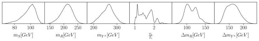
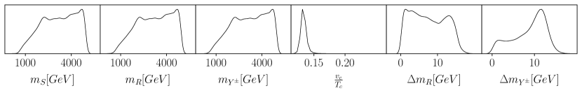
Figure 1: 1-Dimensional posterior distributions from the global fit of the IDM parameters to data. The prior distributions for the mass parameters are flat in the range, [1, 5000] GeV. All model points pass the set of constraints explained in section III. In particular the strength of the first-order EWPT, $\frac{v_{c}}{T_{c}}>1$. The last two plots present the posteriors of the mass splittings between the inert scalars, $\Delta m_{R}=m_{R}-m_{S}$ and $\Delta m_{Y^{\pm}}=m_{Y^{\pm}}-m_{S}$. The second row of plots is the same as the first, but without $\frac{v_{c}}{T_{c}}>1$ imposed.

As is the case for the SM, strong first-order EWPT condition, $\frac{v_{c}}{T_{c}}>1$, translates into an upper bound on the lightest inert Higgs mass. This partly explains way a significant part of the prior region, with $m_{S}\sim 1\,\textrm{to}\,5\,\textrm{TeV}$ will be disfavoured. Should this requirement be uplifted, multi-TeV $m_{S}$ are possible as can be seen on the second row of Figure 1 plots. Imposing the upper limit PandaX-II:2017hlx ; XENON:2019gfn on the inert singlet versus nucleons elastic scattering cross section, $\sigma^{SI}$, on the IDM fit to data leads to small mass differences $\Delta m_{Y^{\pm}}\sim\Delta m_{R}\sim{\cal O}(10)\,\textrm{GeV}$. Contrary to this, the strength of the first-order EWPT, $\frac{v_{c}}{T_{c}}$, is proportional to the mass splittings $\Delta m_{R,\,Y^{\pm}}$. The tendencies with respect to the mass differences can be seen in Figure 2. Therefore, simultaneously requiring both $\frac{v_{c}}{T_{c}}>1$ and the DM direct detection limits on the IDM fit to data is extremely difficult beyond the scope and the computational resources at our disposal. As such, the direct detection limits were not imposed for final fit of the IDM to data since this extremely slowed the sampling of the model parameter space. Instead, the impact of this limit were assessed via post-processing the posterior samples . Complementary to post-processing, a dedicated fit of the model with DM direct limit imposed but without the strong first-order EWPT requirement could be used for assessing the tension between both observables. The second row of plots Figure 1 were from such an IDM fit with the direct detection 90% C.L. exclusions limits XENON:2018voc ; DarkSide:2018bpj ; PICO:2019vsc ; CRESST:2019jnq imposed. As can be seen, this yields posteriors with $\frac{v_{c}}{T_{c}}<0.1$.

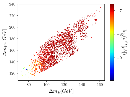
Figure 2: Scatter plots showing the correlations between the inert scalars’ mass differences with: (left) strength of the first-order EWPT, $\frac{v_{c}}{T_{c}}$, and (right) the inert single DM candidate particle’s elastic scattering cross section against nucleons, $\sigma^{SI}$. Both quantities show dependence on the mass differences but in opposite directions with respect to the required respective limits.

The constraints from collider limits disfavours small values of $m_{S}$ and $m_{Y^{\pm}}$, and also contribute to the control that leads to the allowed region for $\Delta m_{R,\,Y^{\pm}}$. This particularly important for the oblique parameters constraints which favour relatively lower inert Higgs mass differences. In all, there are IDM points that satisfy collider and dark matter searches limits including relic density generation, and simultaneously allow for a strong first-order EWPT. A selection of benchmarks are presented in Table 2.

$m_{S}$	$m_{R}$	$m_{Y^{\pm}}$	$\Lambda_{1}$	$\log\,(\Omega_{DM}\,h^{2})$	$\log(\sigma^{SI}[pb])$	$\frac{v_{c}}{T_{c}}$	$\Delta m_{R}$	$\Delta m_{Y^{\pm}}$
93.6989	176.7693	213.3181	0.2853	-2.10594	-8.6287	1.0761	83.0704	119.619
115.0309	133.2492	209.0929	0.3971	-3.64282	-9.28878	1.2038	18.2183	94.0621
101.5063	157.1630	216.7150	0.3678	-3.36139	-9.72497	1.2374	55.6567	115.209
122.3877	198.1699	260.3158	0.4478	-3.26165	-10.8541	1.5127	75.7821	137.928
80.5285	151.8615	193.4262	0.28262	-2.19879	-12.0729	1.0923	71.333	112.898

Table 2: A selection of benchmark points for the IDM model which passed all the constraints considered. Masses are in GeV units.

V Conclusion

We have made a detailed exploration of the parameters and the interplay amongst them for the inert Higgs doublet model in light of the limits from collider experiments, the constraints from dark matter searches and the requirement for a strong first-order electroweak phase transition (EWPT). The software packages BSMPT and micrOMEGAs were used for computing the strength of EWPT and dark matter properties respectively. The collider constraints on the IDM parameter space were applied by using HiggsBounds and Lilith packages. Our analyses include the first global fit of the IDM to data using a statistically convergent Bayesian approach implemented in MultiNest package. For these, we have used, also for the first time, a recently presented most general renormalisable potential for the IDM. This will lead to different phase transition dynamics and coupling constants.

The global fits show that the IDM spectra can have DM candidates with all constraints satisfied and at the same time able to produce a strongly first-order EWPT. A selection of benchmark points was provided which can be analysed further with respect to ongoing or future collider experiments. The posterior sample  could be useful for addressing IDM collider and dark matter phenomenology. Given computing resources, the chain of particle physics phenomenology tools developed can be used for comparisons amongst the extended Higgs sector BSMs in the light EWPT and dark matter candidate particle constraints.

There are several interesting research directions that could be built on the result presented here. Besides the S and T parameters constrained already applied for the fits, there already are interesting collider results from the LHC which could possibly probe further the IDM parameters space. For instance, at the LHC, the electroweak production of $Y^{\pm}$ and $S$ (or $R$) can subsequently lead to the inert Higgs decays into a weak boson and the lightest inert scalar. These can provide the same final states and therefore can be constrained by limits from supersymmetric electroweakino searches ATLAS:2021moa ; ATLAS:2021yqv . Implementing such limits on the IDM will, however, require dedicated reinterpretation studies. The fits revealed strong correlations between three important constraints ($\sigma^{SI}[pb]$, $\frac{v_{c}}{T_{c}}$, and the electroweak precision oblique parameters S and T) used with a strong dependence on the IDM Higgs mass differences albeit with possible pulls along opposing directions. A better delineation of the IDM with respect to these constraints can be achieved by using machine-learning techniques in exploring the compatible regions in parameter space.

Acknowledgements:

We would like to thank Philip Basler for his kind help with the BSMPT package, Alexander Belyaev for advice on the LanHep package and all developers of micrOMEGAs package for their help. MM would like to thank Najimuddin Khan for discussions about perturbative unitarity, Per Osland for the discussions about oblique parameters. This work was partly performed using resources provided by the Cambridge Service for Data Driven Discovery (CSD3) operated by the University of Cambridge Research Computing Service (www.csd3.cam.ac.uk), provided by Dell EMC and Intel using Tier-2 funding from the Engineering and Physical Sciences Research Council (capital grant EP/T022159/1), and DiRAC funding from the Science and Technology Facilities Council (www.dirac.ac.uk).

Appendix A The IDM finite temperature effective potential

The 1-loop finite temperature effective potential for the IDM can br written as follows, following the BSMPT 1803.02846 ; 2007.01725 notations, in terms static field configuration $\omega$ and temperature T.

$$V(\omega,T)=V(\omega)+V_{T}(\omega,T)=V_{tree}(\omega)+V_{CW}(\omega)+V_{CT}(\omega)+V_{T}(\omega,T)$$ (22)

where $V(\omega)$ consists of the tree-level potential $V_{tree}$, Eq.(II), the Coleman-Weinberg potential $V_{CW}$ and the counter-term potential $V_{CT}$. The thermal corrections to the potential is given by $V_{T}(\omega,T)$. In this section we briefly describe each of these terms and then how they are implemented into the BSMPT package in Appendix B.

The notation of Camargo-Molina:2016moz is used for casting the effective potential into the form

$$-\mathcal{L}_{S} =L^{i}\Phi_{i}+\frac{1}{2!}L^{ij}\Phi_{i}\Phi_{j}+\frac{1}{3!}L^{ijk}\Phi_{i}\Phi_{j}\Phi_{k}+\frac{1}{4!}L^{ijkl}\Phi_{i}\Phi_{j}\Phi_{k}\Phi_{l}$$ (23)

$$-\mathcal{L}_{F} =\frac{1}{2}Y^{IJk}\Psi_{I}\Psi_{J}\Phi_{k}+c.c.$$ (24)

$$\mathcal{L}_{G} =\frac{1}{4}G^{abij}A_{a\mu}A_{b}^{\mu}\Phi_{i}\Phi_{j}\;,$$ (25)

with summation over repeated indices implied if one is up and the other is down. In this manner, the IDM scalar multiplets are decomposed into $n_{\text{Higgs}}$ real scalar fields $\Phi_{i}$, with $i=1,\dots,n_{\text{Higgs}}=8$. Here $\Psi_{I}$, with $I=1,\dots,n_{\text{fermion}}$ represents the Weyl fermion multiplets of the model. The four-vectors $A_{\mu}^{a}$, where the index $a$ runs over $n_{\text{gauge}}$ gauge bosons in the adjoint representation of the corresponding gauge group, denotes the gauge bosons of the model. $-\mathcal{L}_{S}$ denotes the extended Higgs potential (including the SM Higgs parts). This consists of the terms $L^{i},L^{ij},L^{ijk},L^{ijkl}$ and the real scalar fields $\Phi_{i}$, with $i,j,k,l=1,\dots,n_{\text{Higgs}}$. $Y^{IJk}$, with $I,J=1\dots n_{\text{fermion}}$, are the couplings for the interactions between the scalar and the fermionic fields. $G^{abij}$, with $a,b=1\dots n_{\text{gauge}}$, are the couplings for the interactions between the scalar and the bosonic fields.

After symmetry breaking the scalar fields are expanded around there VEVs, $\omega_{i}$ as

$$\Phi_{i}(x)=\omega_{i}+\phi_{i}(x).$$ (26)

Putting Eq. (26) in Eqs. (23)-(25) gives

$$-\mathcal{L}_{S} =\Lambda+\Lambda^{i}_{(S)}\phi_{i}+\frac{1}{2}-\Lambda_{(S)}^{ij}\phi_{i}\phi_{j}+\frac{1}{3!}\Lambda^{ijk}_{(S)}-\phi_{i}\phi_{j}\phi_{k}+\frac{1}{4!}-\Lambda_{(S)}^{ijkl}\phi_{i}\phi_{j}\phi_{k}\phi_{l}$$ (27)

$$-\mathcal{L}_{F} =\frac{1}{2}M^{IJ}\Psi_{I}\Psi_{J}+\frac{1}{2}-Y^{IJk}\Psi_{I}\Psi_{J}\phi_{k}+c.c.$$ (28)

$$\mathcal{L}_{G} =\frac{1}{2}\Lambda^{ab}_{(G)}A_{a\mu}A_{b}^{\mu}-+\frac{1}{2}\Lambda^{abi}_{(G)}A_{a\mu}A_{b}^{\mu}\phi_{i}+-\frac{1}{4}\Lambda^{abij}_{(G)}A_{a\mu}A_{b}^{\mu}\phi_{i}\phi_{j}\;,$$ (29)

where

$$\Lambda =V^{(0)}(\omega_{i})=L^{i}\omega_{i}+\frac{1}{2!}L^{ij}\omega_{i}\omega_{j}+\frac{1}{3!}L^{ijk}\omega_{i}\omega_{j}\omega_{k}+\frac{1}{4!}L^{ijkl}\omega_{i}\omega_{j}\omega_{k}\omega_{l}$$ (30)

$$\Lambda_{(S)}^{i} =L^{i}+L^{ij}\omega_{j}+\frac{1}{2}L^{ijk}\omega_{j}\omega_{k}+\frac{1}{6}L^{ijkl}\omega_{j}\omega_{k}\omega_{l}\,,\quad\Lambda_{(S)}^{ij}=L^{ij}+L^{ijk}\omega_{k}+\frac{1}{2}L^{ijkl}\omega_{k}\omega_{l},$$ (31)

$$\Lambda_{(S)}^{ijk} =L^{ijk}+L^{ijkl}\omega_{l}\,,\quad\Lambda_{(S)}^{ijkl}=L^{ijkl}\,,\quad\Lambda_{(G)}^{ab}=\frac{1}{2}G^{abij}\omega_{i}\omega_{j}\,,\quad\Lambda_{(G)}^{abi}=G^{abij}\omega_{j}$$ (32)

$$\Lambda_{(G)}^{abij} =G^{abij}$$ (33)

$$\Lambda_{(F)}^{IJ} =M^{\ast IL}M_{L}^{\;J}=Y^{\ast ILk}Y_{L}^{\;Jm}\omega_{k}\omega_{m}\;,\quad\mbox{with}M^{IJ}=Y^{IJk}\omega_{k}.$$ (34)

We compute each of the terms $\omega_{i},\,L^{i},\,L^{ij},\,L^{ijk},\,L^{ijkl},\,G^{abij}$ and $Y^{IJk}$ in C++ format and then develop the IDM model files needed for BSMPT to work.

The Coleman-Weinberg part of the effective potential

Radiative quantum corrections affects the vacuum structure of potentials at the loop levels. This is accounted for using the 1-loop correction known as Coleman-Weinberg potential Coleman:1973jx given by

$$V_{CW}(\omega)=\frac{1}{4\,\left(4\pi\right)^{2}}\sum_{X={S,G,F}}(-1)^{2s_{X}}(1+2s_{X})Tr[(\Lambda^{xy}_{(X)})^{2}(\log(\frac{1}{\mu^{2}}\Lambda^{xy}_{(X)})-k_{X})],$$ (36)

where $s_{X}$ represents the spin of the field $X$. $X=S,G$ and $F$, respectively, represent scalar, gauge and fermionic fields. The indices $xy$ correspond to the scalar indices $ij$, the gauge indices $ab$ and the fermion indices $IJ$ for $X=S,G$ and $F$, respectively. The sum over $X$ is for all degrees of freedom including colour for the quarks. $\Lambda_{(S)}^{ij}$, $\Lambda_{(G)}^{ab}$ and $\Lambda_{(F)}^{IJ}$ are as given in Eqs. (31), (32) and  (34). The $\overline{\mbox{MS}}$ renormalisation scheme constants are

$$k_{X}=\left\{\begin{array}[]{ll}\frac{5}{6}\;,&\quad\mbox{for gauge bosons}\\[2.84544pt] \frac{3}{2}\;,&\quad\mbox{otherwise}\end{array}\right.$$ (37)

The renormalisation scale $\mu$ is set to the SM Higgs multiplet VEV at $T=0$, $\mu=v(T=0)\approx 246.22\textrm{ GeV}$.

The counter term part of the effective potential

The BSMPT package was designed to use loop-corrected masses and mixing angles as input. As such, the $\overline{\mbox{MS}}$ renormalisation scheme used for the Coleman-Weinberg part of the effective potential has to the modified into the on-shell renormalisation scheme. It is for this reason that the counter term part of the effective potential, $V_{\text{CT}}$, is added. $V_{\text{CT}}$ is obtained by replacing bare parameters $p^{(0)}$ of the tree-level potential $V^{(0)}$ by the renormalised ones, $p$, and their corresponding counter terms $\delta p$

$$V^{\text{CT}} =\sum_{i=1}^{n_{p}}\frac{\partial V^{(0)}}{\partial p_{i}}\delta p_{i}+\sum_{k=1}^{n_{v}}\delta T_{k}\left(\phi_{k}+\omega_{k}\right).$$ (38)

Here $n_{p}$ is the number of parameters of the potential. $\delta T_{k}$ represent the counter terms of the tadpoles $T_{k}$corresponding to the $n_{v}$ directions in field space with non-zero VEV.

The thermal corrections

The temperature dependent part of the effective potential $V^{(T)}$ is given by Dolan:1973qd ; Quiros:1999jp

$$V^{T}(\omega,T) =\sum{X={S,G,F}}{}(-1)^{2s_{X}}(1+2s_{X})\frac{T^{4}}{2\pi^{2}}J_{\pm}\left(\Lambda^{xy}_{(X)}/T^{2}\right)\,,$$ (39)

where $J_{\pm}$ is for bosons or fermions respectively,

$$J_{\pm}\left(\Lambda_{(X)}^{xy}/T^{2}\right) =\textrm{Tr}\left[\int_{0}^{\infty}\,dk\,k^{2}\log\left[1\pm\exp\left(-\sqrt{k^{2}+\Lambda^{xy}_{(X)}/T^{2}}\right)\right]\right]\,.$$ (40)

Taking the finite temperature effect, the daisy corrections Carrington:1991hz to the scalar and gauge boson masses are also implemented in the BSMPT package for the IDM model.

Appendix B Implementation of the IDM model to BSMPT

New models can be implemented in BSMPT. For the IDM, the Lagrangian density terms are written in the required format as described in Appendix A. Using $\Phi_{i}=\{h,x_{1},x_{2},x_{3},y_{1},y_{2},S,R\}$, the code needs $\left\{L^{i},L^{ij},L^{ijk},L^{ijkl},Y^{IJk},G^{abij}\right\}$ as in Eqs. (23), (24), and (25) specified in C++ form. For instance $L^{ij}=0$ unless for $i=j$ for which we have:

$$L^{i,j=x_{3}}=L^{i,j=x_{2}}=L^{i,j=x_{1}}=L^{i,j=h}=-\mu^{2}_{h}$$ (41)

$$L^{i,j=R}=L^{i,j=S}=L^{i,j=y_{2}}=L^{i,j=y_{1}}=\mu^{2}_{Q}.$$ (42)

The same has to be done for the counter terms

$$V^{CT}=\delta\mu^{2}_{h}H^{\dagger}H+\delta\mu^{2}_{Q}Q^{\dagger}Q+\delta\lambda_{1}\left(H^{\dagger}H\right)^{2}+\delta\lambda_{2}[(QQ)_{1}(\overline{Q}\,\overline{Q})_{1}]_{0}+\delta\alpha(H^{\dagger}H)(Q^{\dagger}Q)+$$

$$\delta\beta[(\overline{H}H)_{1}(\overline{Q}Q)_{1}]_{0}+\Big{\{}\delta\kappa_{1}[(HH)_{1}(\overline{Q}\,\overline{Q})_{1}]_{0}+H.c.\Big{\}}+\delta T\left(h+\textrm{VEV}\right).$$ (43)

In order to add this part of the IDM effective Lagrangian to the BSMPT package, the coefficients $\left\{L^{i},L^{ij},L^{ijk},L^{ijkl},Y^{IJk},G^{abij}\right\}$ have to be computed symbolically and then written in C++ form. Applying on-shell renormalisation leads to the equations

$$\left.\partial_{\phi_{i}}V^{\text{CT}}\right|_{\phi=\langle\phi^{c}\rangle_{T=0}} = -\left.\partial_{\phi_{i}}V^{\text{CW}}\right|_{\phi=\langle\phi^{c}\rangle_{T=0}}$$ (44)

$$\left.\partial_{\phi_{i}}\partial_{\phi_{j}}V^{\text{CT}}\right|_{\phi=\langle\phi^{c}\rangle_{T=0}} = -\left.\partial_{\phi_{i}}\partial_{\phi_{j}}V^{\text{CW}}\right|_{\phi=\langle\phi^{c}\rangle_{T=0}}.\$$ (45)

Solving these equations with respect to the counter terms gives

$$\delta\mu^{2}_{h} = -\frac{1}{2}H^{\text{CW}}_{h,h}+\frac{3}{2}H^{\text{CW}}_{x_{3},x_{3}}$$ (46)

$$\delta\mu^{2}_{Q} = -\frac{1}{2}H^{\text{CW}}_{y_{2},y_{2}}-\frac{1}{4}H^{\text{CW}}_{S,S}-\frac{1}{4}H^{\text{CW}}_{R,R}$$ (47)

$$\delta\lambda_{1} = \frac{1}{2v^{2}}\left(-H^{\text{CW}}_{h,h}+H^{\text{CW}}_{x_{3},x_{3}}\right)$$ (48)

$$\delta\lambda_{2} = 0$$ (49)

$$\delta K = \frac{-\sqrt{3}}{2v^{2}}\left(H^{\text{CW}}_{S,S}+H^{\text{CW}}_{R,R}\right)$$ (50)

$$\delta\alpha = 0$$ (51)

$$\delta\beta = \frac{\sqrt{3}}{v^{2}}\left(H^{\text{CW}}_{S,S}+H^{\text{CW}}_{R,R}-2H^{\text{CW}}_{y_{2},y_{2}}\right)$$ (52)

$$\delta T = vH^{\text{CW}}_{x_{3},x_{3}}-N^{\text{CW}}_{h}$$ (53)

Finally for models with a different Yukawa and gauge sectors relative to the SM ones, the thermal corrections codes of the BSMPT has to be modified. For the IDM, the gauge sector differs. To account for this, we modified the function CalculateDebyeGaugeSimplified() using

$$\Pi_{(G)}^{ab}=T^{2}\frac{2}{3}\left(\frac{\tilde{n}_{H}}{8}+5\right)\frac{1}{\tilde{n}_{H}}\sum\limits{m=1}{n_{\text{Higgs}}}\Lambda^{aamm}_{(G)}\delta_{ab}$$ (54)

where $\Pi_{(G)}^{ab}$ belongs to daisy correction to thermal masses of gauge bosons, $\tilde{n}_{H}$ represents the number of Higgs bosons coupled to the SM gauge sector. For the IDM, this leads to

$$\Pi^{a,b=W_{0}}_{G}=\Pi^{a,b=W_{1}}_{G}=\Pi^{a,b=W_{2}}_{G}=2g^{2}$$ (55)

$$\Pi^{a,b=B_{0}}_{G}=2{g^{\prime}}^{2}$$ (56)

where, $g$ and $g^{\prime}$ are SM $SU(2)_{L}$ and $U(1)$ gauge couplings.

References

- (1) A. D. Sakharov, Pisma Zh. Eksp. Teor. Fiz. 5 (1967), 32-35 doi:10.1070/PU1991v034n05ABEH002497
- (2) V. A. Kuzmin, V. A. Rubakov and M. E. Shaposhnikov, Phys. Lett. B 155 (1985), 36 doi:10.1016/0370-2693(85)91028-7
- (3) R. J. Scherrer and M. S. Turner, Phys. Rev. D 33 (1986), 1585 [erratum: Phys. Rev. D 34 (1986), 3263] doi:10.1103/PhysRevD.33.1585
- (4) V. Silveira and A. Zee, Phys. Lett. B 161 (1985), 136-140 doi:10.1016/0370-2693(85)90624-0
- (5) C. P. Burgess, M. Pospelov and T. ter Veldhuis, Nucl. Phys. B 619 (2001), 709-728 doi:10.1016/S0550-3213(01)00513-2 [arXiv:hep-ph/0011335 [hep-ph]].
- (6) M. Cirelli, N. Fornengo and A. Strumia, Nucl. Phys. B 753 (2006), 178-194 doi:10.1016/j.nuclphysb.2006.07.012 [arXiv:hep-ph/0512090 [hep-ph]].
- (7) M. Aoki, S. Kanemura and O. Seto, Phys. Rev. D 80 (2009), 033007 doi:10.1103/PhysRevD.80.033007 [arXiv:0904.3829 [hep-ph]].
- (8) K. Cheung, Y. L. S. Tsai, P. Y. Tseng, T. C. Yuan and A. Zee, JCAP 10 (2012), 042 doi:10.1088/1475-7516/2012/10/042 [arXiv:1207.4930 [hep-ph]].
- (9) D. E. Morrissey and M. J. Ramsey-Musolf, New J. Phys. 14 (2012), 125003 doi:10.1088/1367-2630/14/12/125003 [arXiv:1206.2942 [hep-ph]].
- (10) N. Blinov, S. Profumo and T. Stefaniak, JCAP 07 (2015), 028 doi:10.1088/1475-7516/2015/07/028 [arXiv:1504.05949 [hep-ph]].
- (11) A. Belyaev, G. Cacciapaglia, I. P. Ivanov, F. Rojas-Abatte and M. Thomas, Phys. Rev. D 97 (2018) no.3, 035011 doi:10.1103/PhysRevD.97.035011 [arXiv:1612.00511 [hep-ph]].
- (12) C. W. Chiang, Y. T. Li and E. Senaha, Phys. Lett. B 789 (2019), 154-159 doi:10.1016/j.physletb.2018.12.017 [arXiv:1808.01098 [hep-ph]].
- (13) P. Athron et al. [GAMBIT], Eur. Phys. J. C 79 (2019) no.1, 38 doi:10.1140/epjc/s10052-018-6513-6 [arXiv:1808.10465 [hep-ph]].
- (14) W. Chao, G. J. Ding, X. G. He and M. Ramsey-Musolf, JHEP 08 (2019), 058 doi:10.1007/JHEP08(2019)058 [arXiv:1812.07829 [hep-ph]].
- (15) D. Y. Liu, C. Cai, Z. H. Yu, Y. P. Zeng and H. H. Zhang, JHEP 10 (2020), 212 doi:10.1007/JHEP10(2020)212 [arXiv:2008.06821 [hep-ph]].
- (16) P. Bandyopadhyay and S. Jangid, [arXiv:2111.03866 [hep-ph]].
- (17) Y. Z. Fan, T. P. Tang, Y. L. S. Tsai and L. Wu, Phys. Rev. Lett. 129 (2022) no.9, 9 doi:10.1103/PhysRevLett.129.091802 [arXiv:2204.03693 [hep-ph]].
- (18) N. Khan and S. Rakshit, “Constraints on inert dark matter from the metastability of the electroweak vacuum,” Phys. Rev. D 92, 055006 (2015) doi:10.1103/PhysRevD.92.055006 [arXiv:1503.03085 [hep-ph]].
- (19) A. Datta, N. Ganguly, N. Khan and S. Rakshit, “Exploring collider signatures of the inert Higgs doublet model,” Phys. Rev. D 95, no.1, 015017 (2017) doi:10.1103/PhysRevD.95.015017 [arXiv:1610.00648 [hep-ph]].
- (20) S. S. AbdusSalam and T. A. Chowdhury, JCAP 05 (2014), 026 doi:10.1088/1475-7516/2014/05/026 [arXiv:1310.8152 [hep-ph]].
- (21) N. G. Deshpande and E. Ma, Phys. Rev. D 18 (1978), 2574 doi:10.1103/PhysRevD.18.2574
- (22) L. Fromme, S. J. Huber and M. Seniuch, JHEP 11 (2006), 038 doi:10.1088/1126-6708/2006/11/038 [arXiv:hep-ph/0605242 [hep-ph]].
- (23) Q. H. Cao, E. Ma and G. Rajasekaran, Phys. Rev. D 76 (2007), 095011 doi:10.1103/PhysRevD.76.095011 [arXiv:0708.2939 [hep-ph]].
- (24) R. Barbieri, L. J. Hall and V. S. Rychkov, Phys. Rev. D 74 (2006), 015007 doi:10.1103/PhysRevD.74.015007 [arXiv:hep-ph/0603188 [hep-ph]].
- (25) P. A. Zyla et al. [Particle Data Group], PTEP 2020 (2020) no.8, 083C01 doi:10.1093/ptep/ptaa104
- (26) T. Aaltonen et al. [CDF], Science 376 (2022) no.6589, 170-176 doi:10.1126/science.abk1781
- (27) [CMS], CMS-PAS-TOP-20-008.
- (28) J. de Blas, M. Pierini, L. Reina and L. Silvestrini, [arXiv:2204.04204 [hep-ph]].
- (29) R. Barate et al. [LEP Working Group for Higgs boson searches, ALEPH, DELPHI, L3 and OPAL], Phys. Lett. B 565 (2003), 61-75 doi:10.1016/S0370-2693(03)00614-2 [arXiv:hep-ex/0306033 [hep-ex]].
- (30) [CMS], CMS-PAS-HIG-14-037.
- (31) [CMS], CMS-PAS-HIG-17-013.
- (32) [CMS], CMS-PAS-HIG-21-001.
- (33) X. Miao, S. Su and B. Thomas, Phys. Rev. D 82 (2010), 035009 doi:10.1103/PhysRevD.82.035009 [arXiv:1005.0090 [hep-ph]].
- (34) L. Lopez Honorez and C. E. Yaguna, JHEP 09 (2010), 046 doi:10.1007/JHEP09(2010)046 [arXiv:1003.3125 [hep-ph]].
- (35) A. Ilnicka, M. Krawczyk and T. Robens, Phys. Rev. D 93 (2016) no.5, 055026 doi:10.1103/PhysRevD.93.055026 [arXiv:1508.01671 [hep-ph]].
- (36) T. A. Chowdhury, M. Nemevsek, G. Senjanovic and Y. Zhang, JCAP 02 (2012), 029 doi:10.1088/1475-7516/2012/02/029 [arXiv:1110.5334 [hep-ph]].
- (37) D. Borah and J. M. Cline, Phys. Rev. D 86 (2012), 055001 doi:10.1103/PhysRevD.86.055001 [arXiv:1204.4722 [hep-ph]].
- (38) G. Gil, P. Chankowski and M. Krawczyk, Phys. Lett. B 717 (2012), 396-402 doi:10.1016/j.physletb.2012.09.052 [arXiv:1207.0084 [hep-ph]].
- (39) J. M. Cline and K. Kainulainen, Phys. Rev. D 87 (2013) no.7, 071701 doi:10.1103/PhysRevD.87.071701 [arXiv:1302.2614 [hep-ph]].
- (40) A. Goudelis, B. Herrmann and O. Stål, JHEP 09 (2013), 106 doi:10.1007/JHEP09(2013)106 [arXiv:1303.3010 [hep-ph]].
- (41) M. Gustafsson, S. Rydbeck, L. Lopez-Honorez and E. Lundstrom, Phys. Rev. D 86 (2012), 075019 doi:10.1103/PhysRevD.86.075019 [arXiv:1206.6316 [hep-ph]].
- (42) B. Swiezewska and M. Krawczyk, [arXiv:1305.7356 [hep-ph]].
- (43) E. Dolle, X. Miao, S. Su and B. Thomas, Phys. Rev. D 81 (2010), 035003 doi:10.1103/PhysRevD.81.035003 [arXiv:0909.3094 [hep-ph]].
- (44) D. Dercks and T. Robens, Eur. Phys. J. C 79 (2019) no.11, 924 doi:10.1140/epjc/s10052-019-7436-6 [arXiv:1812.07913 [hep-ph]].
- (45) S. Banerjee, F. Boudjema, N. Chakrabarty, G. Chalons and H. Sun, Phys. Rev. D 100 (2019) no.9, 095024 doi:10.1103/PhysRevD.100.095024 [arXiv:1906.11269 [hep-ph]].
- (46) S. Fabian, F. Goertz and Y. Jiang, JCAP 09 (2021), 011 doi:10.1088/1475-7516/2021/09/011 [arXiv:2012.12847 [hep-ph]].
- (47) M. Aoki, T. Komatsu and H. Shibuya, [arXiv:2106.03439 [hep-ph]].
- (48) B. Eiteneuer, A. Goudelis and J. Heisig, Eur. Phys. J. C 77 (2017) no.9, 624 doi:10.1140/epjc/s10052-017-5166-1 [arXiv:1705.01458 [hep-ph]].
- (49) A. Semenov, Comput. Phys. Commun. 201 (2016), 167-170 doi:10.1016/j.cpc.2016.01.003 [arXiv:1412.5016 [physics.comp-ph]].
- (50) G. Belanger, F. Boudjema, A. Pukhov and A. Semenov, Comput. Phys. Commun. 185 (2014), 960-985 doi:10.1016/j.cpc.2013.10.016 [arXiv:1305.0237 [hep-ph]].
- (51) G. Belanger, F. Boudjema, A. Pukhov and A. Semenov, Nuovo Cim. C 033N2 (2010), 111-116 doi:10.1393/ncc/i2010-10591-3 [arXiv:1005.4133 [hep-ph]].
- (52) G. Belanger, F. Boudjema, A. Pukhov and A. Semenov, Comput. Phys. Commun. 180 (2009), 747-767 doi:10.1016/j.cpc.2008.11.019 [arXiv:0803.2360 [hep-ph]].
- (53) G. Belanger, F. Boudjema, A. Pukhov and A. Semenov, Comput. Phys. Commun. 176 (2007), 367-382 doi:10.1016/j.cpc.2006.11.008 [arXiv:hep-ph/0607059 [hep-ph]].
- (54) P. Basler and M. Mühlleitner, Comput. Phys. Commun. 237 (2019), 62-85 doi:10.1016/j.cpc.2018.11.006 [arXiv:1803.02846 [hep-ph]].
- (55) K. Kannike, Eur. Phys. J. C 72 (2012), 2093 doi:10.1140/epjc/s10052-012-2093-z [arXiv:1205.3781 [hep-ph]].
- (56) I. F. Ginzburg and I. P. Ivanov, Phys. Rev. D 72 (2005), 115010 doi:10.1103/PhysRevD.72.115010 [arXiv:hep-ph/0508020 [hep-ph]].
- (57) P. Bechtle, O. Brein, S. Heinemeyer, G. Weiglein and K. E. Williams, Comput. Phys. Commun. 181 (2010), 138-167 doi:10.1016/j.cpc.2009.09.003 [arXiv:0811.4169 [hep-ph]].
- (58) P. Bechtle, O. Brein, S. Heinemeyer, G. Weiglein and K. E. Williams, Comput. Phys. Commun. 182 (2011), 2605-2631 doi:10.1016/j.cpc.2011.07.015 [arXiv:1102.1898 [hep-ph]].
- (59) P. Bechtle, D. Dercks, S. Heinemeyer, T. Klingl, T. Stefaniak, G. Weiglein and J. Wittbrodt, Eur. Phys. J. C 80 (2020) no.12, 1211 doi:10.1140/epjc/s10052-020-08557-9 [arXiv:2006.06007 [hep-ph]].
- (60) [LEP Higgs Working Group for Higgs boson searches], [arXiv:hep-ex/0107034 [hep-ex]].
- (61) [LEP Higgs Working for Higgs boson searches, ALEPH, DELPHI, L3 CERN and OPAL], [arXiv:hep-ex/0107032 [hep-ex]].
- (62) [LEP Higgs Working Group for Higgs boson searches, ALEPH, DELPHI, L3 and OPAL], [arXiv:hep-ex/0107031 [hep-ex]].
- (63) G. Abbiendi et al. [OPAL], Eur. Phys. J. C 23 (2002), 397-407 doi:10.1007/s100520200896 [arXiv:hep-ex/0111010 [hep-ex]].
- (64) DELPHI-2002-087 CONF 620.
- (65) G. Abbiendi et al. [OPAL], Eur. Phys. J. C 27 (2003), 311-329 doi:10.1140/epjc/s2002-01115-1 [arXiv:hep-ex/0206022 [hep-ex]].
- (66) J. Abdallah et al. [DELPHI], Eur. Phys. J. C 32 (2004), 475-492 doi:10.1140/epjc/s2003-01469-8 [arXiv:hep-ex/0401022 [hep-ex]].
- (67) G. Abbiendi et al. [OPAL], Eur. Phys. J. C 35 (2004), 1-20 doi:10.1140/epjc/s2004-01758-8 [arXiv:hep-ex/0401026 [hep-ex]].
- (68) J. Abdallah et al. [DELPHI], Eur. Phys. J. C 34 (2004), 399-418 doi:10.1140/epjc/s2004-01732-6 [arXiv:hep-ex/0404012 [hep-ex]].
- (69) P. Achard et al. [L3], Phys. Lett. B 609 (2005), 35-48 doi:10.1016/j.physletb.2005.01.030 [arXiv:hep-ex/0501033 [hep-ex]].
- (70) J. Abdallah et al. [DELPHI], Eur. Phys. J. C 38 (2004), 1-28 doi:10.1140/epjc/s2004-02011-4 [arXiv:hep-ex/0410017 [hep-ex]].
- (71) S. Schael et al. [ALEPH, DELPHI, L3, OPAL and LEP Working Group for Higgs Boson Searches], Eur. Phys. J. C 47 (2006), 547-587 doi:10.1140/epjc/s2006-02569-7 [arXiv:hep-ex/0602042 [hep-ex]].
- (72) G. Abbiendi et al. [OPAL], Phys. Lett. B 682 (2010), 381-390 doi:10.1016/j.physletb.2009.09.010 [arXiv:0707.0373 [hep-ex]].
- (73) G. Abbiendi et al. [OPAL], Eur. Phys. J. C 72 (2012), 2076 doi:10.1140/epjc/s10052-012-2076-0 [arXiv:0812.0267 [hep-ex]].
- (74) G. Abbiendi et al. [ALEPH, DELPHI, L3, OPAL and LEP], Eur. Phys. J. C 73 (2013), 2463 doi:10.1140/epjc/s10052-013-2463-1 [arXiv:1301.6065 [hep-ex]].
- (75) T. Aaltonen et al. [CDF], Phys. Rev. Lett. 102 (2009), 021802 doi:10.1103/PhysRevLett.102.021802 [arXiv:0809.3930 [hep-ex]].
- (76) V. M. Abazov et al. [D0], Phys. Lett. B 671 (2009), 349-355 doi:10.1016/j.physletb.2008.12.009 [arXiv:0806.0611 [hep-ex]].
- (77) V. M. Abazov et al. [D0], Phys. Lett. B 682 (2009), 278-286 doi:10.1016/j.physletb.2009.11.016 [arXiv:0908.1811 [hep-ex]].
- (78) T. Aaltonen et al. [CDF], Phys. Rev. Lett. 103 (2009), 101803 doi:10.1103/PhysRevLett.103.101803 [arXiv:0907.1269 [hep-ex]].
- (79) T. Aaltonen et al. [CDF], Phys. Rev. Lett. 103 (2009), 201801 doi:10.1103/PhysRevLett.103.201801 [arXiv:0906.1014 [hep-ex]].
- (80) V. M. Abazov et al. [D0], Phys. Rev. Lett. 103 (2009), 061801 doi:10.1103/PhysRevLett.103.061801 [arXiv:0905.3381 [hep-ex]].
- (81) V. M. Abazov et al. [D0], Phys. Lett. B 698 (2011), 97-104 doi:10.1016/j.physletb.2011.02.062 [arXiv:1011.1931 [hep-ex]].
- (82) T. Aaltonen et al. [CDF], Phys. Rev. Lett. 104 (2010), 061803 doi:10.1103/PhysRevLett.104.061803 [arXiv:1001.4468 [hep-ex]].
- (83) V. M. Abazov et al. [D0], Phys. Rev. Lett. 104 (2010), 061804 doi:10.1103/PhysRevLett.104.061804 [arXiv:1001.4481 [hep-ex]].
- (84) D. Benjamin et al. [Tevatron New Phenomena & Higgs Working Group], [arXiv:1003.3363 [hep-ex]].
- (85) V. M. Abazov et al. [D0], Phys. Rev. Lett. 105 (2010), 251801 doi:10.1103/PhysRevLett.105.251801 [arXiv:1008.3564 [hep-ex]].
- (86) V. M. Abazov et al. [D0], Phys. Rev. D 84 (2011), 092002 doi:10.1103/PhysRevD.84.092002 [arXiv:1107.1268 [hep-ex]].
- (87) V. M. Abazov et al. [D0], Phys. Lett. B 707 (2012), 323-329 doi:10.1016/j.physletb.2011.12.050 [arXiv:1106.4555 [hep-ex]].
- (88) V. M. Abazov et al. [D0], Phys. Rev. Lett. 107 (2011), 121801 doi:10.1103/PhysRevLett.107.121801 [arXiv:1106.4885 [hep-ex]].
- (89) D. Benjamin [CDF, D0, TEVNPH Working Group (Tevatron New Phenomena and Higgs Working Group)], [arXiv:1108.3331 [hep-ex]].
- (90) [TEVNPH (Tevatron New Phenomina, Higgs Working Group), CDF and D0], [arXiv:1203.3774 [hep-ex]].
- (91) T. Aaltonen et al. [CDF and D0], Phys. Rev. Lett. 109 (2012), 071804 doi:10.1103/PhysRevLett.109.071804 [arXiv:1207.6436 [hep-ex]].
- (92) G. Aad et al. [ATLAS], Phys. Lett. B 716 (2012), 1-29 doi:10.1016/j.physletb.2012.08.020 [arXiv:1207.7214 [hep-ex]].
- (93) G. Aad et al. [ATLAS], Phys. Rev. Lett. 108 (2012), 111802 doi:10.1103/PhysRevLett.108.111802 [arXiv:1112.2577 [hep-ex]].
- (94) G. Aad et al. [ATLAS], Phys. Rev. Lett. 107 (2011), 221802 doi:10.1103/PhysRevLett.107.221802 [arXiv:1109.3357 [hep-ex]].
- (95) G. Aad et al. [ATLAS], Phys. Lett. B 707 (2012), 27-45 doi:10.1016/j.physletb.2011.11.056 [arXiv:1108.5064 [hep-ex]].
- (96) G. Aad et al. [ATLAS], Phys. Lett. B 710 (2012), 383-402 doi:10.1016/j.physletb.2012.03.005 [arXiv:1202.1415 [hep-ex]].
- (97) G. Aad et al. [ATLAS], Phys. Rev. Lett. 108 (2012), 111803 doi:10.1103/PhysRevLett.108.111803 [arXiv:1202.1414 [hep-ex]].
- (98) G. Aad et al. [ATLAS], Phys. Lett. B 710 (2012), 49-66 doi:10.1016/j.physletb.2012.02.044 [arXiv:1202.1408 [hep-ex]].
- (99) G. Aad et al. [ATLAS], JHEP 06 (2012), 039 doi:10.1007/JHEP06(2012)039 [arXiv:1204.2760 [hep-ex]].
- (100) G. Aad et al. [ATLAS], Phys. Lett. B 732 (2014), 8-27 doi:10.1016/j.physletb.2014.03.015 [arXiv:1402.3051 [hep-ex]].
- (101) G. Aad et al. [ATLAS], Phys. Rev. Lett. 112 (2014), 201802 doi:10.1103/PhysRevLett.112.201802 [arXiv:1402.3244 [hep-ex]].
- (102) G. Aad et al. [ATLAS], Phys. Rev. Lett. 113 (2014) no.17, 171801 doi:10.1103/PhysRevLett.113.171801 [arXiv:1407.6583 [hep-ex]].
- (103) G. Aad et al. [ATLAS], JHEP 11 (2014), 056 doi:10.1007/JHEP11(2014)056 [arXiv:1409.6064 [hep-ex]].
- (104) G. Aad et al. [ATLAS], Phys. Lett. B 738 (2014), 68-86 doi:10.1016/j.physletb.2014.09.008 [arXiv:1406.7663 [hep-ex]].
- (105) G. Aad et al. [ATLAS], Phys. Rev. Lett. 114 (2015) no.8, 081802 doi:10.1103/PhysRevLett.114.081802 [arXiv:1406.5053 [hep-ex]].
- (106) G. Aad et al. [ATLAS], JHEP 01 (2016), 032 doi:10.1007/JHEP01(2016)032 [arXiv:1509.00389 [hep-ex]].
- (107) G. Aad et al. [ATLAS], Eur. Phys. J. C 76 (2016) no.4, 210 doi:10.1140/epjc/s10052-016-4034-8 [arXiv:1509.05051 [hep-ex]].
- (108) G. Aad et al. [ATLAS], Eur. Phys. J. C 76 (2016) no.1, 45 doi:10.1140/epjc/s10052-015-3820-z [arXiv:1507.05930 [hep-ex]].
- (109) G. Aad et al. [ATLAS], Phys. Rev. Lett. 114 (2015) no.23, 231801 doi:10.1103/PhysRevLett.114.231801 [arXiv:1503.04233 [hep-ex]].
- (110) G. Aad et al. [ATLAS], Phys. Lett. B 744 (2015), 163-183 doi:10.1016/j.physletb.2015.03.054 [arXiv:1502.04478 [hep-ex]].
- (111) G. Aad et al. [ATLAS], Phys. Rev. D 92 (2015), 092004 doi:10.1103/PhysRevD.92.092004 [arXiv:1509.04670 [hep-ex]].
- (112) M. Aaboud et al. [ATLAS], JHEP 09 (2016), 173 doi:10.1007/JHEP09(2016)173 [arXiv:1606.04833 [hep-ex]].
- (113) M. Aaboud et al. [ATLAS], Eur. Phys. J. C 76 (2016) no.11, 605 doi:10.1140/epjc/s10052-016-4418-9 [arXiv:1606.08391 [hep-ex]].
- (114) M. Aaboud et al. [ATLAS], JHEP 03 (2018), 042 doi:10.1007/JHEP03(2018)042 [arXiv:1710.07235 [hep-ex]].
- (115) M. Aaboud et al. [ATLAS], Eur. Phys. J. C 78 (2018) no.1, 24 doi:10.1140/epjc/s10052-017-5491-4 [arXiv:1710.01123 [hep-ex]].
- (116) M. Aaboud et al. [ATLAS], Eur. Phys. J. C 78 (2018) no.4, 293 doi:10.1140/epjc/s10052-018-5686-3 [arXiv:1712.06386 [hep-ex]].
- (117) M. Aaboud et al. [ATLAS], JHEP 01 (2018), 055 doi:10.1007/JHEP01(2018)055 [arXiv:1709.07242 [hep-ex]].
- (118) M. Aaboud et al. [ATLAS], Phys. Lett. B 775 (2017), 105-125 doi:10.1016/j.physletb.2017.10.039 [arXiv:1707.04147 [hep-ex]].
- (119) M. Aaboud et al. [ATLAS], Phys. Rev. D 98 (2018) no.5, 052008 doi:10.1103/PhysRevD.98.052008 [arXiv:1808.02380 [hep-ex]].
- (120) M. Aaboud et al. [ATLAS], JHEP 11 (2018), 085 doi:10.1007/JHEP11(2018)085 [arXiv:1808.03599 [hep-ex]].
- (121) M. Aaboud et al. [ATLAS], Phys. Lett. B 783 (2018), 392-414 doi:10.1016/j.physletb.2018.07.006 [arXiv:1804.01126 [hep-ex]].
- (122) M. Aaboud et al. [ATLAS], Phys. Lett. B 790 (2019), 1-21 doi:10.1016/j.physletb.2018.10.073 [arXiv:1807.00539 [hep-ex]].
- (123) M. Aaboud et al. [ATLAS], Eur. Phys. J. C 78 (2018) no.12, 1007 doi:10.1140/epjc/s10052-018-6457-x [arXiv:1807.08567 [hep-ex]].
- (124) M. Aaboud et al. [ATLAS], JHEP 09 (2018), 139 doi:10.1007/JHEP09(2018)139 [arXiv:1807.07915 [hep-ex]].
- (125) M. Aaboud et al. [ATLAS], JHEP 10 (2018), 031 doi:10.1007/JHEP10(2018)031 [arXiv:1806.07355 [hep-ex]].
- (126) M. Aaboud et al. [ATLAS], JHEP 05 (2019), 124 doi:10.1007/JHEP05(2019)124 [arXiv:1811.11028 [hep-ex]].
- (127) M. Aaboud et al. [ATLAS], Phys. Lett. B 793 (2019), 499-519 doi:10.1016/j.physletb.2019.04.024 [arXiv:1809.06682 [hep-ex]].
- (128) M. Aaboud et al. [ATLAS], Phys. Rev. Lett. 121 (2018) no.19, 191801 [erratum: Phys. Rev. Lett. 122 (2019) no.8, 089901] doi:10.1103/PhysRevLett.121.191801 [arXiv:1808.00336 [hep-ex]].
- (129) G. Aad et al. [ATLAS], Phys. Lett. B 801 (2020), 135148 doi:10.1016/j.physletb.2019.135148 [arXiv:1909.10235 [hep-ex]].
- (130) M. Aaboud et al. [ATLAS], Phys. Rev. Lett. 122 (2019) no.23, 231801 doi:10.1103/PhysRevLett.122.231801 [arXiv:1904.05105 [hep-ex]].
- (131) M. Aaboud et al. [ATLAS], JHEP 07 (2019), 117 doi:10.1007/JHEP07(2019)117 [arXiv:1901.08144 [hep-ex]].
- (132) G. Aad et al. [ATLAS], Phys. Lett. B 800 (2020), 135069 doi:10.1016/j.physletb.2019.135069 [arXiv:1907.06131 [hep-ex]].
- (133) G. Aad et al. [ATLAS], Phys. Lett. B 800 (2020), 135103 doi:10.1016/j.physletb.2019.135103 [arXiv:1906.02025 [hep-ex]].
- (134) G. Aad et al. [ATLAS], Phys. Rev. D 102 (2020) no.3, 032004 doi:10.1103/PhysRevD.102.032004 [arXiv:1907.02749 [hep-ex]].
- (135) S. Chatrchyan et al. [CMS], Phys. Rev. Lett. 108 (2012), 111804 doi:10.1103/PhysRevLett.108.111804 [arXiv:1202.1997 [hep-ex]].
- (136) S. Chatrchyan et al. [CMS], JHEP 03 (2012), 040 doi:10.1007/JHEP03(2012)040 [arXiv:1202.3478 [hep-ex]].
- (137) S. Chatrchyan et al. [CMS], JHEP 04 (2012), 036 doi:10.1007/JHEP04(2012)036 [arXiv:1202.1416 [hep-ex]].
- (138) S. Chatrchyan et al. [CMS], Phys. Lett. B 710 (2012), 26-48 doi:10.1016/j.physletb.2012.02.064 [arXiv:1202.1488 [hep-ex]].
- (139) S. Chatrchyan et al. [CMS], Phys. Rev. D 89 (2014) no.9, 092007 doi:10.1103/PhysRevD.89.092007 [arXiv:1312.5353 [hep-ex]].
- (140) S. Chatrchyan et al. [CMS], Phys. Lett. B 726 (2013), 587-609 doi:10.1016/j.physletb.2013.09.057 [arXiv:1307.5515 [hep-ex]].
- (141) S. Chatrchyan et al. [CMS], Phys. Rev. D 89 (2014) no.1, 012003 doi:10.1103/PhysRevD.89.012003 [arXiv:1310.3687 [hep-ex]].
- (142) V. Khachatryan et al. [CMS], Eur. Phys. J. C 74 (2014) no.10, 3076 doi:10.1140/epjc/s10052-014-3076-z [arXiv:1407.0558 [hep-ex]].
- (143) S. Chatrchyan et al. [CMS], Eur. Phys. J. C 74 (2014), 2980 doi:10.1140/epjc/s10052-014-2980-6 [arXiv:1404.1344 [hep-ex]].
- (144) V. Khachatryan et al. [CMS], JHEP 10 (2015), 144 doi:10.1007/JHEP10(2015)144 [arXiv:1504.00936 [hep-ex]].
- (145) V. Khachatryan et al. [CMS], Phys. Lett. B 748 (2015), 221-243 doi:10.1016/j.physletb.2015.07.010 [arXiv:1504.04710 [hep-ex]].
- (146) V. Khachatryan et al. [CMS], JHEP 01 (2016), 079 doi:10.1007/JHEP01(2016)079 [arXiv:1510.06534 [hep-ex]].
- (147) V. Khachatryan et al. [CMS], Phys. Lett. B 750 (2015), 494-519 doi:10.1016/j.physletb.2015.09.062 [arXiv:1506.02301 [hep-ex]].
- (148) V. Khachatryan et al. [CMS], JHEP 11 (2015), 018 doi:10.1007/JHEP11(2015)018 [arXiv:1508.07774 [hep-ex]].
- (149) V. Khachatryan et al. [CMS], Phys. Lett. B 755 (2016), 217-244 doi:10.1016/j.physletb.2016.01.056 [arXiv:1510.01181 [hep-ex]].
- (150) V. Khachatryan et al. [CMS], JHEP 11 (2015), 071 doi:10.1007/JHEP11(2015)071 [arXiv:1506.08329 [hep-ex]].
- (151) V. Khachatryan et al. [CMS], JHEP 12 (2015), 178 doi:10.1007/JHEP12(2015)178 [arXiv:1510.04252 [hep-ex]].
- (152) V. Khachatryan et al. [CMS], Phys. Lett. B 752 (2016), 146-168 doi:10.1016/j.physletb.2015.10.067 [arXiv:1506.00424 [hep-ex]].
- (153) V. Khachatryan et al. [CMS], Phys. Lett. B 749 (2015), 560-582 doi:10.1016/j.physletb.2015.08.047 [arXiv:1503.04114 [hep-ex]].
- (154) V. Khachatryan et al. [CMS], Phys. Lett. B 759 (2016), 369-394 doi:10.1016/j.physletb.2016.05.087 [arXiv:1603.02991 [hep-ex]].
- (155) V. Khachatryan et al. [CMS], Phys. Rev. D 94 (2016) no.5, 052012 doi:10.1103/PhysRevD.94.052012 [arXiv:1603.06896 [hep-ex]].
- (156) A. M. Sirunyan et al. [CMS], Phys. Lett. B 778 (2018), 101-127 doi:10.1016/j.physletb.2018.01.001 [arXiv:1707.02909 [hep-ex]].
- (157) A. M. Sirunyan et al. [CMS], JHEP 01 (2018), 054 doi:10.1007/JHEP01(2018)054 [arXiv:1708.04188 [hep-ex]].
- (158) V. Khachatryan et al. [CMS], JHEP 10 (2017), 076 doi:10.1007/JHEP10(2017)076 [arXiv:1701.02032 [hep-ex]].
- (159) A. M. Sirunyan et al. [CMS], JHEP 11 (2017), 010 doi:10.1007/JHEP11(2017)010 [arXiv:1707.07283 [hep-ex]].
- (160) A. M. Sirunyan et al. [CMS], Phys. Lett. B 793 (2019), 320-347 doi:10.1016/j.physletb.2019.03.064 [arXiv:1811.08459 [hep-ex]].
- (161) A. M. Sirunyan et al. [CMS], JHEP 11 (2018), 115 doi:10.1007/JHEP11(2018)115 [arXiv:1808.06575 [hep-ex]].
- (162) A. M. Sirunyan et al. [CMS], JHEP 11 (2018), 018 doi:10.1007/JHEP11(2018)018 [arXiv:1805.04865 [hep-ex]].
- (163) A. M. Sirunyan et al. [CMS], Phys. Lett. B 795 (2019), 398-423 doi:10.1016/j.physletb.2019.06.021 [arXiv:1812.06359 [hep-ex]].
- (164) A. M. Sirunyan et al. [CMS], Phys. Lett. B 793 (2019), 520-551 doi:10.1016/j.physletb.2019.04.025 [arXiv:1809.05937 [hep-ex]].
- (165) A. M. Sirunyan et al. [CMS], Phys. Lett. B 785 (2018), 462 doi:10.1016/j.physletb.2018.08.057 [arXiv:1805.10191 [hep-ex]].
- (166) A. M. Sirunyan et al. [CMS], JHEP 06 (2018), 127 [erratum: JHEP 03 (2019), 128] doi:10.1007/JHEP06(2018)127 [arXiv:1804.01939 [hep-ex]].
- (167) A. M. Sirunyan et al. [CMS], JHEP 08 (2018), 113 doi:10.1007/JHEP08(2018)113 [arXiv:1805.12191 [hep-ex]].
- (168) A. M. Sirunyan et al. [CMS], Phys. Rev. Lett. 122 (2019) no.12, 121803 doi:10.1103/PhysRevLett.122.121803 [arXiv:1811.09689 [hep-ex]].
- (169) A. M. Sirunyan et al. [CMS], JHEP 09 (2018), 007 doi:10.1007/JHEP09(2018)007 [arXiv:1803.06553 [hep-ex]].
- (170) A. M. Sirunyan et al. [CMS], JHEP 03 (2020), 051 doi:10.1007/JHEP03(2020)051 [arXiv:1911.04968 [hep-ex]].
- (171) A. M. Sirunyan et al. [CMS], Phys. Lett. B 800 (2020), 135087 doi:10.1016/j.physletb.2019.135087 [arXiv:1907.07235 [hep-ex]].
- (172) A. M. Sirunyan et al. [CMS], JHEP 07 (2019), 142 doi:10.1007/JHEP07(2019)142 [arXiv:1903.04560 [hep-ex]].
- (173) A. M. Sirunyan et al. [CMS], JHEP 03 (2020), 034 doi:10.1007/JHEP03(2020)034 [arXiv:1912.01594 [hep-ex]].
- (174) A. M. Sirunyan et al. [CMS], JHEP 03 (2020), 103 doi:10.1007/JHEP03(2020)103 [arXiv:1911.10267 [hep-ex]].
- (175) A. M. Sirunyan et al. [CMS], Phys. Lett. B 798 (2019), 134992 doi:10.1016/j.physletb.2019.134992 [arXiv:1907.03152 [hep-ex]].
- (176) A. M. Sirunyan et al. [CMS], JHEP 04 (2020), 171 doi:10.1007/JHEP04(2020)171 [arXiv:1908.01115 [hep-ex]].
- (177) A. M. Sirunyan et al. [CMS], JHEP 03 (2020), 055 doi:10.1007/JHEP03(2020)055 [arXiv:1911.03781 [hep-ex]].
- (178) A. M. Sirunyan et al. [CMS], Eur. Phys. J. C 79 (2019) no.7, 564 doi:10.1140/epjc/s10052-019-7058-z [arXiv:1903.00941 [hep-ex]].
- (179) A. M. Sirunyan et al. [CMS], JHEP 07 (2020), 126 doi:10.1007/JHEP07(2020)126 [arXiv:2001.07763 [hep-ex]].
- (180) J. Bernon and B. Dumont, Eur. Phys. J. C 75 (2015) no.9, 440 doi:10.1140/epjc/s10052-015-3645-9 [arXiv:1502.04138 [hep-ph]].
- (181) D. Barducci, G. Belanger, J. Bernon, F. Boudjema, J. Da Silva, S. Kraml, U. Laa and A. Pukhov, Comput. Phys. Commun. 222 (2018), 327-338 doi:10.1016/j.cpc.2017.08.028 [arXiv:1606.03834 [hep-ph]].
- (182) S. Kraml, T. Q. Loc, D. T. Nhung and L. Ninh, SciPost Phys. 7 (2019) no.4, 052 doi:10.21468/SciPostPhys.7.4.052 [arXiv:1908.03952 [hep-ph]].
- (183) T. Aaltonen et al. [CDF and D0], Phys. Rev. D 88 (2013) no.5, 052014 doi:10.1103/PhysRevD.88.052014 [arXiv:1303.6346 [hep-ex]].
- (184) G. Aad et al. [ATLAS], Eur. Phys. J. C 76 (2016) no.1, 6 doi:10.1140/epjc/s10052-015-3769-y [arXiv:1507.04548 [hep-ex]].
- (185) G. Aad et al. [ATLAS], Phys. Rev. D 90 (2014) no.11, 112015 doi:10.1103/PhysRevD.90.112015 [arXiv:1408.7084 [hep-ex]].
- (186) G. Aad et al. [ATLAS], JHEP 08 (2015), 137 doi:10.1007/JHEP08(2015)137 [arXiv:1506.06641 [hep-ex]].
- (187) G. Aad et al. [ATLAS], Phys. Rev. D 91 (2015) no.1, 012006 doi:10.1103/PhysRevD.91.012006 [arXiv:1408.5191 [hep-ex]].
- (188) G. Aad et al. [ATLAS], JHEP 04 (2015), 117 doi:10.1007/JHEP04(2015)117 [arXiv:1501.04943 [hep-ex]].
- (189) G. Aad et al. [ATLAS], Phys. Lett. B 749 (2015), 519-541 doi:10.1016/j.physletb.2015.07.079 [arXiv:1506.05988 [hep-ex]].
- (190) G. Aad et al. [ATLAS], Eur. Phys. J. C 75 (2015) no.7, 349 doi:10.1140/epjc/s10052-015-3543-1 [arXiv:1503.05066 [hep-ex]].
- (191) G. Aad et al. [ATLAS], Phys. Lett. B 738 (2014), 68-86 doi:10.1016/j.physletb.2014.09.008 [arXiv:1406.7663 [hep-ex]].
- (192) G. Aad et al. [ATLAS], Phys. Rev. Lett. 112 (2014), 201802 doi:10.1103/PhysRevLett.112.201802 [arXiv:1402.3244 [hep-ex]].
- (193) M. Aaboud et al. [ATLAS], Phys. Rev. D 98 (2018), 052005 doi:10.1103/PhysRevD.98.052005 [arXiv:1802.04146 [hep-ex]].
- (194) M. Aaboud et al. [ATLAS], JHEP 03 (2018), 095 doi:10.1007/JHEP03(2018)095 [arXiv:1712.02304 [hep-ex]].
- (195) M. Aaboud et al. [ATLAS], Phys. Rev. D 99 (2019), 072001 doi:10.1103/PhysRevD.99.072001 [arXiv:1811.08856 [hep-ex]].
- (196) M. Aaboud et al. [ATLAS], Phys. Rev. Lett. 119 (2017) no.5, 051802 doi:10.1103/PhysRevLett.119.051802 [arXiv:1705.04582 [hep-ex]].
- (197) M. Aaboud et al. [ATLAS], Phys. Lett. B 789 (2019), 508-529 doi:10.1016/j.physletb.2018.11.064 [arXiv:1808.09054 [hep-ex]].
- (198) M. Aaboud et al. [ATLAS], Phys. Rev. D 98 (2018) no.5, 052003 doi:10.1103/PhysRevD.98.052003 [arXiv:1807.08639 [hep-ex]].
- (199) M. Aaboud et al. [ATLAS], Phys. Rev. Lett. 122 (2019) no.23, 231801 doi:10.1103/PhysRevLett.122.231801 [arXiv:1904.05105 [hep-ex]].
- (200) G. Aad et al. [ATLAS], Phys. Lett. B 798 (2019), 134949 doi:10.1016/j.physletb.2019.134949 [arXiv:1903.10052 [hep-ex]].
- (201) M. Aaboud et al. [ATLAS], JHEP 12 (2017), 024 doi:10.1007/JHEP12(2017)024 [arXiv:1708.03299 [hep-ex]].
- (202) M. Aaboud et al. [ATLAS], Phys. Lett. B 776 (2018), 318-337 doi:10.1016/j.physletb.2017.11.049 [arXiv:1708.09624 [hep-ex]].
- (203) M. Aaboud et al. [ATLAS], Phys. Rev. D 97 (2018) no.7, 072003 doi:10.1103/PhysRevD.97.072003 [arXiv:1712.08891 [hep-ex]].
- (204) M. Aaboud et al. [ATLAS], Phys. Rev. D 97 (2018) no.7, 072016 doi:10.1103/PhysRevD.97.072016 [arXiv:1712.08895 [hep-ex]].
- (205) V. Khachatryan et al. [CMS], Eur. Phys. J. C 75 (2015) no.5, 212 doi:10.1140/epjc/s10052-015-3351-7 [arXiv:1412.8662 [hep-ex]].
- (206) V. Khachatryan et al. [CMS], Eur. Phys. J. C 74 (2014) no.10, 3076 doi:10.1140/epjc/s10052-014-3076-z [arXiv:1407.0558 [hep-ex]].
- (207) S. Chatrchyan et al. [CMS], JHEP 01 (2014), 096 doi:10.1007/JHEP01(2014)096 [arXiv:1312.1129 [hep-ex]].
- (208) S. Chatrchyan et al. [CMS], Phys. Rev. D 89 (2014) no.9, 092007 doi:10.1103/PhysRevD.89.092007 [arXiv:1312.5353 [hep-ex]].
- (209) S. Chatrchyan et al. [CMS], JHEP 05 (2014), 104 doi:10.1007/JHEP05(2014)104 [arXiv:1401.5041 [hep-ex]].
- (210) S. Chatrchyan et al. [CMS], Phys. Rev. D 89 (2014) no.1, 012003 doi:10.1103/PhysRevD.89.012003 [arXiv:1310.3687 [hep-ex]].
- (211) V. Khachatryan et al. [CMS], JHEP 09 (2014), 087 [erratum: JHEP 10 (2014), 106] doi:10.1007/JHEP09(2014)087 [arXiv:1408.1682 [hep-ex]].
- (212) V. Khachatryan et al. [CMS], Eur. Phys. J. C 75 (2015) no.6, 251 doi:10.1140/epjc/s10052-015-3454-1 [arXiv:1502.02485 [hep-ex]].
- (213) V. Khachatryan et al. [CMS], Phys. Rev. D 92 (2015) no.3, 032008 doi:10.1103/PhysRevD.92.032008 [arXiv:1506.01010 [hep-ex]].
- (214) S. Chatrchyan et al. [CMS], Eur. Phys. J. C 74 (2014), 2980 doi:10.1140/epjc/s10052-014-2980-6 [arXiv:1404.1344 [hep-ex]].
- (215) A. M. Sirunyan et al. [CMS], Eur. Phys. J. C 79 (2019) no.5, 421 doi:10.1140/epjc/s10052-019-6909-y [arXiv:1809.10733 [hep-ex]].
- (216) A. M. Sirunyan et al. [CMS], JHEP 06 (2019), 093 doi:10.1007/JHEP06(2019)093 [arXiv:1809.03590 [hep-ex]].
- (217) A. M. Sirunyan et al. [CMS], Phys. Lett. B 793 (2019), 520-551 doi:10.1016/j.physletb.2019.04.025 [arXiv:1809.05937 [hep-ex]].
- (218) S. Heinemeyer et al. [LHC Higgs Cross Section Working Group], doi:10.5170/CERN-2013-004 [arXiv:1307.1347 [hep-ph]].
- (219) [ATLAS], ATLAS-CONF-2020-052.
- (220) X. Cui et al. [PandaX-II], Phys. Rev. Lett. 119 (2017) no.18, 181302 doi:10.1103/PhysRevLett.119.181302 [arXiv:1708.06917 [astro-ph.CO]].
- (221) E. Aprile et al. [XENON], Phys. Rev. Lett. 123 (2019) no.25, 251801 doi:10.1103/PhysRevLett.123.251801 [arXiv:1907.11485 [hep-ex]].
- (222) N. Aghanim et al. [Planck], Astron. Astrophys. 641 (2020), A6 [erratum: Astron. Astrophys. 652 (2021), C4] doi:10.1051/0004-6361/201833910 [arXiv:1807.06209 [astro-ph.CO]].
- (223) M. Quiros, [arXiv:hep-ph/9901312 [hep-ph]].
- (224) P. Basler and M. Mühlleitner, Comput. Phys. Commun. 237 (2019), 62-85 doi:10.1016/j.cpc.2018.11.006 [arXiv:1803.02846 [hep-ph]].
- (225) P. Basler, M. Mühlleitner and J. Müller, Comput. Phys. Commun. 269 (2021), 108124 doi:10.1016/j.cpc.2021.108124 [arXiv:2007.01725 [hep-ph]].
- (226) F. Feroz and M. P. Hobson, Mon. Not. Roy. Astron. Soc. 384 (2008), 449 doi:10.1111/j.1365-2966.2007.12353.x [arXiv:0704.3704 [astro-ph]].
- (227) F. Feroz, M. P. Hobson and M. Bridges, Mon. Not. Roy. Astron. Soc. 398 (2009), 1601-1614 doi:10.1111/j.1365-2966.2009.14548.x [arXiv:0809.3437 [astro-ph]].
- (228) E. Aprile et al. [XENON], Phys. Rev. Lett. 121 (2018) no.11, 111302 doi:10.1103/PhysRevLett.121.111302 [arXiv:1805.12562 [astro-ph.CO]].
- (229) P. Agnes et al. [DarkSide], Phys. Rev. Lett. 121 (2018) no.8, 081307 doi:10.1103/PhysRevLett.121.081307 [arXiv:1802.06994 [astro-ph.HE]].
- (230) C. Amole et al. [PICO], Phys. Rev. D 100 (2019) no.2, 022001 doi:10.1103/PhysRevD.100.022001 [arXiv:1902.04031 [astro-ph.CO]].
- (231) A. H. Abdelhameed et al. [CRESST], Phys. Rev. D 100 (2019) no.10, 102002 doi:10.1103/PhysRevD.100.102002 [arXiv:1904.00498 [astro-ph.CO]].
- (232) J. E. Camargo-Molina, A. P. Morais, R. Pasechnik, M. O. P. Sampaio and J. Wessén, JHEP 08 (2016), 073 doi:10.1007/JHEP08(2016)073 [arXiv:1606.07069 [hep-ph]].
- (233) S. R. Coleman and E. J. Weinberg, Phys. Rev. D 7 (1973), 1888-1910 doi:10.1103/PhysRevD.7.1888
- (234) L. Dolan and R. Jackiw, Phys. Rev. D 9 (1974), 3320-3341 doi:10.1103/PhysRevD.9.3320
- (235) M. E. Carrington, Phys. Rev. D 45 (1992), 2933-2944 doi:10.1103/PhysRevD.45.2933
- (236) G. Aad et al. [ATLAS], Eur. Phys. J. C 81 (2021) no.12, 1118 doi:10.1140/epjc/s10052-021-09749-7 [arXiv:2106.01676 [hep-ex]].
- (237) G. Aad et al. [ATLAS], Phys. Rev. D 104 (2021) no.11, 112010 doi:10.1103/PhysRevD.104.112010 [arXiv:2108.07586 [hep-ex]].