Estimating Probability Distributions of Travel Times
by Fitting a Markovian Velocity Model

Abstract.

To improve the routing decisions of individual drivers and the management policies designed by traffic operators, one needs reliable estimates of travel time distributions. Since congestion caused by both recurrent patterns (e.g., rush hours) and non-recurrent events (e.g., traffic incidents) leads to potentially substantial delays in highway travel times, we focus on a framework capable of incorporating both effects. To this end, we propose to work with the Markovian velocity model, based on an environmental background process that tracks both random and (semi-)predictable events affecting the vehicle speeds in a highway network. We show how to operationalize this flexible data-driven model in order to obtain the travel time distribution for a vehicle departing at a known day and time to traverse a given path. Specifically, we detail how to structure the background process and set the speed levels corresponding to the different states of this process. First, for the inclusion of non-recurrent events, we study incident data to describe the random durations of the incident and inter-incident times. Both of them depend on the time of day, but we identify periods in which they can be considered time-independent. Second, for an estimation of the speed patterns in both incident and inter-incident regime, loop detector data for each of the identified periods is studied. In numerical examples that use road network detector data of the Dutch highway network, we obtain the travel time distribution estimates that arise under different traffic regimes, and illustrate the advantages compared to traditional travel-time prediction methods.

Keywords. Travel time distribution $\circ$ Markovian background process $\circ$ Incident duration $\circ$ Recurrent congestion $\circ$ Loop detector data.

Affiliations. NL and MM are with the Korteweg-de Vries Institute for Mathematics, University of Amsterdam, Amsterdam. MB is with the Department of Mathematics and Computer Science, Eindhoven University of Technology, Eindhoven. MB and MM are also with Eurandom, Eindhoven, and MM with Amsterdam Business School, University of Amsterdam, Amsterdam. This research project is partly funded by the NWO Gravitation project Networks, grant number 024.002.003. Date: March 13, 2024.

Copyright notice. This work has been submitted to the IEEE for possible publication. Copyright may be transferred without notice, after which this version may no longer be accessible.

1. Introduction

Motivation and short method description
Accurate and efficient estimation of travel time distributions is needed to help individual travelers make well-informed routing decisions. Moreover, traffic operators use information about travel time distributions for the design of optimal policies for traffic management. Consequently, a reliable description of these travel times may lead to reductions of delays, economic costs, and $\text{CO}_{2}$ emissions. Considering vehicle trip times, one should distinguish between so-called recurrent congestion (i.e., near-periodic effects, such as congestion during peak hour) and non-recurrent congestion (which is inherently less predictable, e.g. covering congestion due to incidents) potentially contributing to substantial delays. When aiming at describing travel time distributions, it is therefore essential to include both effects. The objective of this paper is to develop, in the context of a highway network, a framework for capturing the impact of recurrent and non-recurrent congestion.

Since the origins of recurrent congestion are of an essentially periodic nature, it follows a highly predictable pattern. This can be inferred from velocity data, often available through the loop detectors or speed cameras present in traffic networks. In contrast, incidents are considerably less predictable, both in terms of location and severity. Our work focuses on developing a description of the randomness regarding such incidents, and a quantification of their impact on highway travel times, in a model that in addition takes the recurrent, near-periodic effects into account. In our approach we incorporate events that directly impact the velocities at which the vehicles can drive (which we refer to as ‘driveable speed levels’), thus ignoring second-order effects that are caused by the driving style that individual drivers may have.

We demonstrate our approach by studying traffic data from the Dutch highway network, which we use to get a handle on the (random) incident lengths, inter-incident times and corresponding driveable speed levels. The analysis employs loop detector data, in combination with a database of registered incidents. While we use the Dutch data in our ‘proof of concept’, our techniques can be applied to any highway network for which similar data sets are available. Importantly, with the results of the analysis, we operationalize the Markovian velocity model (mvm), as was introduced in Levering et al. (2022). This stochastic model uses an environmental background process to track both recurrent and non-recurrent events affecting vehicle speeds in a road network, and outputs, given its departure day and time, a description of the travel time of a vehicle traversing a specific path. Notably, this description yields an accurate proxy for the distribution of this travel time, rather than just a ‘point estimate’, thereby providing insight into the impact of the random effects discussed above. With increasing recognition of travel time reliability as an important performance measure, such distributions serve as input for a line of routing studies that take the risk-averseness of users into account (see e.g. Fosgerau and Karlström (2010)).

A main reason for our choice to use the mvm to model travel time distributions lies in the fact that it is ‘velocity oriented’ and data-driven. In addition, it is remarkably flexible in terms of its capacity to include the various sources of travel time fluctuations. Concretely, the proposed framework transparently captures the causes of recurrent as well as non-recurrent congestion in a single model. Indeed, we can incorporate near-deterministic events (such as the onset of the rush hour, or the duration of the rush hour), as well as events of an intrinsically more random nature (such as incidents). Moreover, the underlying mechanism is rich enough to allow for correlation between the speeds on different segments in the network, present due to e.g. spillback and rubbernecking after incidents. Lastly, as is demonstrated in this paper, despite the flexibility the model offers, it can be made operational with relatively low complexity, which makes it directly useful for practical purposes. One such practical application of the mvm is studied in Levering et al. (2022), who employ the model in an optimal routing context, in which an individual vehicle wishes to minimize its expected travel time between a given origin and destination.

Literature review
Since incidents potentially have a dramatic impact on highway travel times, their duration has been studied extensively. Some early works describe the randomness of incident durations by the lognormal distribution (Garib et al., 1997, Giuliano, 1989, Sullivan, 1997). Reviews of more recent studies (Chung and Yoon, 2012, Li et al., 2018) reveal that, besides the lognormal distribution, the log-logistic and Weibull distribution are frequently found to describe the random duration of incidents well. Li et al. (2018) distinguish between the analysis and prediction of traffic incidents. On the one hand, analysis studies have the objective to determine which factors have a significant impact on the incident duration. Types of factors that are found to affect the duration include environmental conditions, the characteristics of the incident, and traffic flow conditions. On the other hand, prediction studies have the objective to forecast the duration of a current incident. Reviewed prediction methods are e.g. regression models, artificial neural networks, and hazard-based duration models.

An important remark is that the applicability of the incident distributions reported in Chung and Yoon (2012) and Li et al. (2018) is limited for the description of future incidents. First, these studies do not consider the incident rate (i.e., the rate at which a new incident occurs), and are therefore unable to describe the time until a future incident. Second, incident durations are often modeled under various configurations of explanatory variables, but information regarding the values of these factors may only be available if an incident has actually occurred, or even only if an incident has elapsed for a certain period of time (e.g. number of involved vehicles, number of closed lanes). Thus, since these prediction methods are only useful once this information becomes available, they are of limited use for predicting the duration of future incidents or incidents that just occurred. The latter case is also studied by Khattak et al. (1995) and Ghosh et al. (2019), who account for the chronological availability of information by presenting a time-sequential prediction method that updates the prediction when new information becomes available. Importantly, for current incidents, the mvm model that we advocate in this paper offers the same flexibility, while additionally being able to describe the time until and the duration of future incidents.

The Markovian velocity model of Levering et al. (2022) includes current incidents, future incidents, and daily patterns in the travel time distribution, by capturing the effect of recurrent and non-recurrent events on highway speeds. In contrast to most travel time prediction methods (see e.g. the summaries in van Hinsbergen et al. (2007), Vlahogianni et al. (2014) and Qiu and Fan (2021)), the model outputs a distribution of the travel time rather than a point estimate, so as to provide insight in the impact of traffic incidents. Moreover, it is one of the few models that directly models the impact of traffic incidents on travel times. That is, most studies regarding travel time distributions focus solely on daily patterns, and describe the travel time distribution for different periods of day. Examples of such recent studies include Chalumuri and Yasuo (2014), Guessous et al. (2014), Chen and Fan (2019) and Chen and Fan (2020). In the data-driven models of Filipovska et al. (2021), both daily patterns and incidents are incorporated, but, as they investigate general path travel time distributions, there is no focus towards incidents that are in the network at the moment of the vehicle’s departure.

To the best of our knowledge, two of the few studies that assess the impact of current incidents on the travel time are the regression models presented by Tavassoli Hojati et al. (2016) and Javid and Javid (2018). However, the impact of the incident on the travel time is only indirectly quantified, as the models use a travel time reliability measure as response variable. Similarly, Xie et al. (2020) do not directly investigate travel times during incidents, but focus on the problem of incident-driven speed prediction, and, to this end, propose the use of a specific graph convolutional network. Miller and Gupta (2012) do consider the incident-induced delay directly, but only predict the incident impact as a class variable.

The Markov model of Levering et al. (2022) is a natural extension of the travel time models presented by Kim et al. (2005a, b), Yeon et al. (2008) and Güner et al. (2012). These studies use a Markovian background process to model the daily recurrent patterns and let the state of the process on a link directly impact the travel time on this link, thereby neglecting spatial correlation. In contrast, besides daily patterns, the background process in Levering et al. (2022) is used to model more complex traffic events, such as traffic incidents, and recognizes the correlation between link travel times. Moreover, similar to Kharoufeh and Gautam (2004), the travel time adheres the FIFO-property, as the state of the continuous background process impacts the driveable vehicle speed instead of the travel time.

Main contributions
The contributions of this paper are twofold. In the first place, we demonstrate how traffic data can be used to obtain an accurate description of the randomness of incidents. This description involves the incidents’ frequency, duration and impact on traffic velocities. These turn out to typically depend on the time of day and day of week, but one can deal with these fluctuations by working with periods over which these effects are essentially constant. As mentioned above, the data study concerns the Dutch highway network, but our techniques extend to all highway networks for which incident and speed data is available.

In the second place, we show how to include both the randomness of incidents and the recurrent traffic patterns, so as to obtain the travel time distribution of a vehicle traversing a path through the network. Concretely, we use the results from the data study to operationalize the mvm, thus tracking both (near-deterministic) time-dependent and intrinsically random events. We explicitly show how incidents and daily patterns can be incorporated into the background process, and how their effect on vehicle speeds must be chosen to accurately reflect their impact on the travel time of a vehicle. By doing so, we provide traffic management centers and individual drivers with a transparent modelling framework, which they can easily calibrate to their needs, so as to obtain travel time distribution estimates.

Paper organization

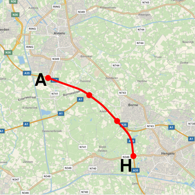
(a) A35 highway path between Almelo and Hengelo.

(b) Graphical scheme. Nodes represent ramps, the indexed directed links the highway parts between the ramps.

Figure 1. Path Almelo-Hengelo

The mvm is compactly described in Section 2. Section 3 starts with a description of the considered network and corresponding traffic data, to then continue with an analysis of this data for arcs in both the incident and non-incident setting. Section 4 details how the observations from the data analysis can be used to operationalize the mvm. Numerical examples of the resulting travel time distributions are given in Section 5. Section 6 contains concluding remarks.

2. Markovian velocity model

The main objective of this section is to briefly describe the Markovian velocity model (mvm), as developed in Levering et al. (2022), which we propose to use for the prediction of travel time distributions. As touched upon in the introduction, our choice for the mvm stems from the transparency and extreme flexibility it offers for the modeling of both recurrent and non-recurrent traffic events, in terms of their frequency, duration, and their impact on network velocities. Indeed, from a data study of the Dutch highway network (Section 3), it will become apparent that the mvm framework is well capable of describing the vehicle speeds in this network. It is important to note that we focus on the (recurrent and non-recurrent) events that directly affect the speed levels the vehicles can drive at. This concretely means that our approach does not incorporate velocity-impacting effects due to e.g. the individual drivers’ heterogeneity in driving style.

The mvm uses a background process, or environment process, to track the near-deterministic and random events affecting the vehicle speeds in the road network. Section 2.1 provides an illustrative example for the structure of this background process, when considering a vehicle traversing a path in a small network with typical traffic events. A more detailed description of the mathematical framework of the mvm is presented in Section 2.2. In Section 2.3 we discuss general principles underlying statistically fitting traffic events.

2.1. Modeling example

Consider a vehicle that intends to traverse the A35 highway in the Netherlands between Almelo and Hengelo (Figure 1), and that enters this highway in Almelo at a moment at which there is no reported incident. Figure 1 shows the graph that corresponds to the path, with each node representing a ramp on the highway, and each link representing the highway part between two of these ramps. As in the rest of this paper, we are interested in the travel time of the vehicle planning to traverse the path, given the vehicle enters this path at a specific day and time.

Observe that the travel time a vehicle experiences can be inferred from the speeds the vehicle is able to drive. On the considered part of the A35 highway, the maximum speed as set by the Dutch government equals 100 km/h. However, the attained speed on the arcs is not necessarily this maximum. In reality, events such as rush hour and traffic incidents lead to fluctuations in vehicle speeds. To model these effects, the mvm introduces a background process that tracks the events affecting the speeds.

A prominent source of speed variability is formed by randomly occurring traffic incidents. To model these incidents, we let $\{X_{i}(t),t\!\geq\!0\}$ be a continuous-time Markov process that records whether there is an incident on link $i$ at time $t$. Specifically, we choose

$$X_{i}(t) =\begin{cases}1&\quad\quad\text{if there is an incident on arc $i$ at time $t$,}\\ 2&\quad\quad\text{otherwise},\end{cases}\quad\text{ and }\quad Q_{i}=\begin{bmatrix}-\alpha_{i}&\alpha_{i}\\ \beta_{i}&-\beta_{i}\end{bmatrix},$$

with $Q_{i}$ the transition rate matrix of $X_{i}(t)$ with transition rates $\alpha_{i},\beta_{i}>0$. Thus, in this example, we observe that $X_{i}(t)$ is a process that cyclically switches between an exponentially distributed time (with mean $1/\alpha_{i}$) during which there is an incident on arc $i$, and an exponentially distributed incident-free time (with mean $1/\beta_{i}$). We let, for different links $i$ and $j$, the processes $X_{i}(t)$ and $X_{j}(t)$ evolve independently. Then, the superimposed process $B(t):=(X_{1}(t),\dots,X_{6}(t))$ is a Markovian background process recording the incidents in the network of Figure 1, having a state space of dimension $2^{6}$. Setting $t\!=\!0$ as the time the vehicle enters the A35 highway at Almelo, we know $B(0)\!=\!(2,2,\dots,2)$, as there were no reported incidents at that time.

Figure 2. Example of speed levels (in km/h) on the A35 highway between Almelo (A) and Hengelo (H), in case of (a) no incidents, (b) an incident on link 3. The latter shows the effect of spillback and rubbernecking.

Now, if, during the traversal of the path between Almelo and Hengelo, an incident would occur at one of the links, naturally, the speed level on this link is affected by the incident. An important observation is that the impact on vehicle speeds may not be limited to the incident link itself. That is, potential spillback and rubbernecking effects may lead to speed reductions on upstream links or the link on the other side of the barrier as well. To reflect this dependence, we let the velocity on an arc be determined by the complete state of the background process $B(t)$. Concretely, if $B(t)$ is in state $s\!\in\!\{1,2\}^{6}$, the vehicle speed at arc $i$ equals $v_{i}(s)$. Indeed, modeling the speeds in this fashion, the speed on link $i$ does not solely depend on $X_{i}(t)$, but is allowed to depend on all $X_{j}(t),\leavevmode\nobreak\ j\!=\!1,\dots,6$. Thus, if we would want to capture the typical traffic behavior during an incident at link 3, with estimated speed levels as displayed in Figure 2, we could simply set the speeds in state $s=(2,2,1,2,2,2)$ equal to $(v_{1}(s),v_{2}(s),v_{3}(s),v_{4}(s),v_{5}(s),v_{6}(s))\!=\!(60,100,30,80,100,100)$.

Besides incidents, there may be other traffic events that have a severe impact on the speeds the vehicle can drive. For example, consider the situation that between $t\!=\!15$ and $t\!=\!30$ precipitation is forecasted. Note that, typically, precipitation does not just affect the speeds around one link, but has impact on a larger area of the network. Now, to include these weather conditions in the background process $B(t)$, we simply extend $B(t)$ by an additional Markov process $Y(t)$ that describes whether at time $t$ the precipitation has not yet started (encoded by $Y(t)\!=\!1$), currently falls ($Y(t)\!=\!2$) or has already stopped ($Y(t)\!=\!3$). The three states are visited successively (Figure 3), with $Y(t)\!=\!1$ at $t\!=\!0$. The extension of $B(t)$ allows us to define the speed levels on the arcs, again, by letting the velocity on an arc $i$ equal $v_{i}(s)$ whenever $B(t)\!=\!s$. We have thus constructed the background process $B(t):=(X_{1}(t),\dots,X_{6}(t),Y(t))$ with $2^{6}\cdot 3$ states.

Remark 1.

In the above example, we model, for simplicity, the durations of the first two states of $Y(t)$ by exponential distributions. However, as we will argue in Section 2.3, the mvm framework is not restrictive, in the sense that we can work with a considerably more general class of distributions. Importantly, these phase-type distributions can accommodate random quantities that are both less and more variable than the exponential distribution, thus making the setup highly flexible. $\hfill\Diamond$

Figure 3. Structure of $Y(t)$ describing the precipitation pattern, with $\lambda_{1}=\lambda_{2}=1/15$.

Notably, the precipitation may not only impact the driveable speed levels on the arcs, but may, additionally, impact the incident rate on the arcs (Bergel-Hayat et al., 2013). Therefore, we allow the transition rates of the processes $X_{i}(t)$ to depend on the state of $Y(t)$. Then, with $Q_{y}$ the transition rate matrix of $(X_{1}(t),\dots,X_{6}(t))$ in case $Y(t)=y\in\{1,2,3\}$, the $(2^{6}\cdot 3)\times(2^{6}\cdot 3)$-dimensional transition rate matrix $Q$ of the background process $B(t)$ is of the form

$$Q=\begin{bmatrix}Q_{1}\!-\!\lambda_{1}I&\lambda_{1}I&\\ &Q_{2}\!-\!\lambda_{2}I&\lambda_{2}I\\ &&Q_{3}\end{bmatrix},$$

with $\lambda_{1}$ and $\lambda_{2}$ as in Figure 3.

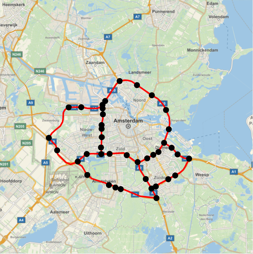
Figure 4. Amsterdam highway network, with nodes representing ramps, and links representing the two directed arcs between these ramps.

In case traffic incidents and the upcoming precipitation are the only events potentially affecting arc speeds, the full travel time distribution of the considered vehicle can be derived from the presented random speed dynamics. Indeed, given we know the state of the background process upon departure from Almelo, the above formalism specifies the distribution of the time it takes to arrive in Hengelo. Evidently, if there are additional sources of variability, the background process can be extended to include these events as well. Details on the general structure of $B(t)$ are given in the mathematical model description below.

2.2. Mathematical model description

After having introduced various concepts in our illustrative example, let us now consider a general road network, encoded by its corresponding graph representation $G=(N,A)$, of which the set of nodes $N$ represents the ramps in the road network, and the set of directed arcs $A$ represents the roads connecting these ramps. Hence, $k\ell\in A$ only if the ramps represented by the nodes $k$ and $\ell$ are subsequent ramps on one (directed) road. A small example is the path-network between Almelo-Hengelo, as shown in Figure 1. An example network of more realistic size, the highway network around Amsterdam, the Netherlands, is displayed in Figure 4. Note that splitting highways at the ramps allows the model to be used for practical applications such as the routing of individual vehicles. In the rest of this paper, both the terms arc and link refer to a highway part that arises by this splitting procedure, i.e., a piece of highway enclosed by two ramps. In case we consider a highway part enclosed by two highway intersections, we will use the term highway segment. Note that, with every intersection being a ramp but not vice versa, a highway segment can always be partitioned into highway links.

In reality, the driveable speed level on the link $k\ell\in A$ is not necessarily constant. As argued, events such as incidents and heavy rainfall lead to fluctuations in the speeds vehicles can drive at. As illustrated in the modeling example above, the mvm captures this randomness in vehicle speeds by the introduction of an environmental background process $B(t)$ on the arcs $A$, which keeps track of the events affecting the arc speeds. To this end, the mvm distinguishes three types of events: (i) recurrent events, (ii) random incidents, and (iii) the (semi-)predictable non-recurrent traffic events that are either present at the vehicle’s departure or known to occur in the foreseeable future (e.g. forecasted snowfall, road work). We will refer to the third type of events as scheduled events.

Let $n:=|A|$, and write $A=\{a_{1},\dots,a_{n}\}$ for the set of arcs in $G$, with $a_{i}:=k_{i}\ell_{i}$ for some $k_{i},\ell_{i}\in N$. To model traffic incidents, our primary focus, we define $\{X_{a_{i}}(t),t\geqslant 0\}$ as independent Markov processes such that for $a_{i}\in A$:

$$X_{a_{i}}(t) =\begin{cases}1&\quad\quad\text{if there is an incident on arc $a_{i}$ at time $t$,}\\ 2&\quad\quad\text{otherwise}.\end{cases}$$

Then, the Markovian background process $B(t)$ recording the ‘incident status’ of the full network $G$ is given by $(X_{a_{1}}(t),\dots,X_{a_{n}}(t))$. We let the velocity of a vehicle traversing $a_{i}$ be determined by the background process $B(t)$ in the following way: if $B(t)$ is in state $s\in\{1,2\}^{n}$, the speed at which vehicles are moving on the arc is $v_{a_{i}}(s)$. This way, the speed on arc $a_{i}$ is allowed to depend on all processes $X_{a_{1}}(t),\dots,X_{a_{n}}(t)$. Notably, the possibility to model correlation between speeds on different arcs is an important asset of the mvm, as it can be used to model real-world traffic phenomena like the spillback effect.

Note that the current structure of the processes $X_{a_{i}}(t)$ is such that there are only two states for the modeling of incidents and their impact on arc speeds. We are, however, by no means restricted to this two-state structure: we could allow $X_{a_{i}}(t)$ to be any continuous-time Markov process. This gives us the opportunity to model more complex incident speed patterns (e.g. distinguishing the incident itself, a recovery phase, and the regular conditions), and additionally provides flexibility for the distribution of the incident length (i.e., this distribution is no longer strictly exponential; see Remark 1). Thus, we let $X_{a_{i}}(t)$ be a continuous-time Markov process that represents the state of an incident at arc $a_{i}\in A$ at time $t$, and set $B(t)=(X_{a_{1}}(t),\dots,X_{a_{n}}(t))$, with $X_{a_{i}}(t),X_{a_{j}}(t)$ evolving independently for $i\!\leavevmode\nobreak\ \neq\!\leavevmode\nobreak\ j$. Dependence between the arc speeds is again realized by allowing the velocity on each arc to depend on the state of the vector $B(t)$: if $B(t)=s$ the velocity at which vehicles are moving on arc $a_{j}$ is $v_{a_{j}}(s)$.

To include the two other types of events, the recurrent and the scheduled events, we expand the background process $B(t)$ with a Markov process $Y(t)$. Specifically, in case there are $m$ scheduled events, $Y(t)$ is structured as $(Y_{0}(t),Y_{1}(t),\dots,Y_{m}(t))$, with $Y_{0}(t)$ a Markov process that models the effect of the recurrent, daily traffic patterns, and $Y_{1}(t),\dots,Y_{m}(t)$ Markov processes that model the $m$ scheduled events (of which the process in Figure 3 is an example). As noted in the illustrative example of Section 2.1, recurrent and scheduled events may not just impact the driveable speeds in the network, but may, additionally, impact the transition rates of the processes $X_{a_{i}}(t)$. For example, for an arc in the network, there may be a significant difference between the inter-incident time within and outside the rush hours. Therefore, we let $B(t)=(Y(t),X_{a_{1}}(t),\dots,X_{a_{n}}(t))$ be such that only conditional on the state of the ‘common process’ $Y(t)$, the individual processes $X_{a_{i}}(t)$ (for $i=1,\ldots,n$) evolve independently.

Now, in case the background process $B(t)$ for a departing vehicle is fully specified, i.e., all background states and transition rates are known, the travel time distribution is fully specified as well. That is, if $B(t)$ is in state $s$ at the departure time of the vehicle, the travel time on an edge $a_{i}$ with length $d_{a_{i}}$ is distributed as $\tau^{s}_{a_{i}}$, with

$$\tau_{a_{i}}^{s}:=\min\left\{t\geqslant 0:\left.\int_{0}^{t}v_{a_{i}}(B(u))\,{\rm d}u\geqslant d_{a_{i}}\>\right|\,B(0)=s\right\}.$$

An expression for the Laplace-Stieltjes transform (LST) of $\tau^{s}_{a_{i}}$ was derived Levering et al. (2022). Importantly, the LST of a non-negative random variable uniquely determines its distribution function, and, moreover, the derivatives of the LST yield the moments of the random variable.

2.3. Fitting traffic events

One of the advantages of the mvm framework is its flexibility, in the sense that it allows a high degree of generality when it comes to the distributions of the durations of the underlying events. It is true that the times spent in the states of a continuous-time Markov process necessarily follow exponential distributions, but, as briefly mentioned in Remark 1, the mvm is still capable of handling non-exponential distributions. That is, if data analysis would reveal either the duration of an event affecting arc speeds, or the duration between two such events, to be non-exponential, we can use phase-type distributions to cast these durations into the Markovian setting, and, as a result, include the event(s) into the mvm. Importantly, phase-type distributions have the attractive property that they can model random quantities that are less variable than the exponential distribution as well as random quantities that are more variable than the exponential distribution. In the remainder of this subsection we provide more background.

Informally, the class of phase-type (PH) random variables consists of all sums and mixtures of exponentially distributed random variables. This concretely means that any phase-type distribution is characterized by a Markov process with $d\!+\!1$ states, an entrance probability vector $\bm{\alpha}\in\mathbb{R}^{d+1}$, and a transition rate matrix of the form

$$Q_{\rm PH}=\begin{pmatrix}T&-T\bm{1}\\ \bm{0}^{\top}&0\\ \end{pmatrix},$$

with $T\in\mathbb{R}^{d\times d}$, and $\bm{0}$ and $\bm{1}$ respectively denoting all zeroes and all ones $d$-dimensional column vectors; see (Asmussen, 2003, Section III.4). The transient states $1,\dots,d$ are the so-called phases of the Markov process. From the structure of the transition matrix $Q_{\rm PH}$, we note that state $d\!+\!1$ is an absorbing state. With the random variable $X$ denoting the total elapsed time from the start of the described Markov process until absorption in $d\!+\!1$, we say that $X$ has a PH($\bm{\alpha},Q_{\rm PH}$) distribution. From this definition, it is immediately clear that we can include any traffic event with a PH duration into our framework. Instead of working with a single phase, as we did in the above examples with exponentially distributed durations, we now include the $d$ phases of the PH distribution into our model. Concretely, when the event starts, the initial phase is sampled according to $\bm{\alpha}$, after which the Markov process $X$ evolves according to $Q_{\rm PH}$ until a transition to the absorption state occurs. Then the background process of the mvm moves to one of the outdegree neighbors belonging to the event under consideration, according to their respective transition rates.

We already mentioned that phase-type distributions can model non-negative random quantities that differ in variability from the exponential distribution. We proceed by making this claim more precise. To obtain an approximating distribution for such a random quantity $X$, it is common procedure to use the two-moment phase-type matching approximation that was advocated by Tijms (1986). The underlying principle is to fit a phase-type distribution to the mean $\mathbb{E}[X]$ and the squared coefficient of variation $c_{X}^{2}$, defined as:

$$c_{X}^{2} =\frac{\text{Var}(X)}{\mathbb{E}[X]^{2}}=\frac{\mathbb{E}[X^{2}]}{\mathbb{E}[X]^{2}}-1.$$

Note that the SCV of an exponentially distributed random variable equals 1. The fitting procedure distinguishes two cases:

• In case $0\!<\!c_{X}^{2}\!<\!1$, the distribution of $X$ is less variable than the exponential distribution. In this case $X$ is approximated by a mixture of Erlang distributions. That is, the fitted distribution is with probability $p$ an Erlang distribution with $k\!-\!1$ phases and mean $(k\!-\!1)/\mu$, and with probability $1\!-\!p$ an Erlang distribution with $k$ phases and mean $k/\mu$. A simple calculation shows that the SCV of this distribution equals $(k-p^{2})/(k-p)^{2}$, which for $p\in[0,1]$ lies between $1/k$ and $1/(k\!-\!1)$. Hence, we set $k$ such that $1/k\!\leq\!c_{X}^{2}\!\leq\!1/(k\!-\!1)$. Both $\mu$ and $p$ are now chosen such that the mean and the SCV of the mixture Erlang distribution uniquely match $\mathbb{E}[X]$ and $c_{X}^{2}$.

• In case $c_{X}^{2}\!\geq 1$, the distribution of $X$ is more variable than the exponential distribution. In this case $X$ is approximated by a hyperexponential distribution, which equals an exponential($\mu_{1}$) distribution with probability $p$, and an exponential($\mu_{2}$) distribution with probability $1\!-\!p$. In this setting, the three parameters cannot be uniquely determined from $\mathbb{E}[X]$ and $c_{X}^{2}$. However, this can be tackled by imposing balanced means, i.e., using the normalization $p/\mu_{1}=(1\!-\!p)/\mu_{2}$, which reduces the number of free parameters from three to two.

(a) Exponential precipitation duration.

(b) Mixture Erlang precipitation duration.

Figure 5. Modeling the precipitation length, instead of with an exponential distribution (a), with a mixture Erlang distribution (b).

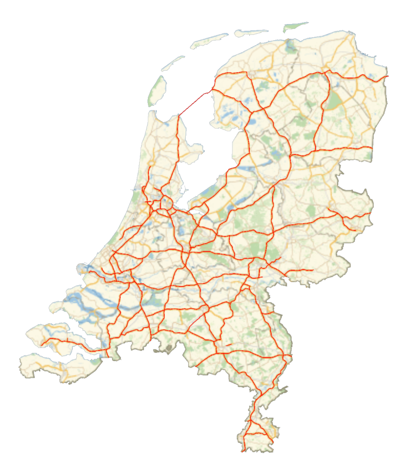
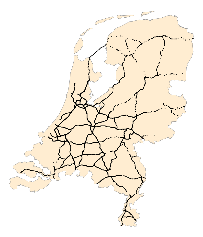
Figure 6. The segments (above) and loop detectors (below) in the Dutch highway system.

A small example for the implementation of phase-type distributions in $B(t)$ is provided in Figure 5. We consider the forecasted precipitation from Section 2.1, whose impact was described by a Markov process with successive states 1, 2 and 3, respectively denoting the time before, during and after the precipitation (Figure 5a). Consequently, both the time until the precipitation and the duration of the precipitation are modeled by exponential distributions. However, if statistical analysis and the above fitting procedure reveal that the duration of the precipitation is better described by a mixture of an exponential distribution and the sum of two exponential distributions, we can include this PH distribution by replacing state 2 by the three phases of this distribution (Figure 5b).

3. Speed pattern analysis in the Dutch highway network

This section investigates daily speed patterns, and, in particular, the impact of traffic incidents on these driveable vehicle speeds. The study focuses on the Dutch highway network, for which extensive data sets on traffic jams and vehicle speeds are openly available (Section 3.1). Importantly, use of the Dutch data is merely illustrative, as the techniques we present can be applied to any highway network for which similar data sets are accessible. Now, to describe the traffic patterns in the Dutch network, we investigate, for all individual segments, the random durations and attained velocities in both the inter-incident (Section 3.2) and the incident regimes (Section 3.3). It turns out that these durations and corresponding speed levels depend on the time of day and day of week, but that there are periods in which these effects are relatively constant.

In principle, the insights of this section can be used in any model describing vehicle speeds. The mvm of Section 2 is an example of such a model, and we will argue that the findings of the present section indeed align with the mvm. To this end, we already include some remarks in the present section that reveal how the observed speed patterns can be incorporated in the mvm. More detail is provided in Section 4, in which we further specify the fitting procedure, and highlight how to construct the background process of the mvm corresponding to the Dutch highway network.

3.1. Network and data description

The Dutch highway network, depicted in Figure 6, consists of all highways (i.e., the so-called A-roads) in the Netherlands. In our analysis, we additionally include three non-highway trajectories, that each serve as important connection between two highways. Now, to study the speed levels in this network, we split each of these roads into highway segments, i.e., highway parts separated by highway interchanges. Hence, each network segment we consider is either a directed road between two highway interchanges, or the first or last section of a highway. Splitting at the interchanges allows the use of the results for the travel time estimation of vehicles traversing paths consisting of multiple highways. Moreover, splitting a highway into a larger number of segments implies that an even larger amount of data will be required for a meaningful analysis of the incident impact.

(a) Location

(b) Time of day

Figure 7. Dependence of number of registered incidents ($n$) in the years 2015-2019 on location and time of the day.

We study traffic data of the Dutch highway network to predict the impact of traffic events on the velocities at the highway segments. Specifically, we assess the incident duration, the time between incidents, and the vehicle speeds in both these settings. For the analysis, two openly available data sets are used: (i) a database with traffic speeds and flows at loop detectors in the Dutch road network and (ii) a list of registered traffic jams. In the Netherlands, these two data sources are managed by the National Road Traffic Data Portal (ndw) and Rijkswaterstaat (rws), respectively.

The ndw data set (NDW, 2020) contains loop detector data from the year 2017. On most Dutch highways, there is a high concentration of loop detectors, as can be noted from their locations as shown in Figure 6. Every minute, the average traffic flow and speed at these loops are registered and stored.

The rws data set (Rijkswaterstaat, 2015) contains all registered traffic jams from the year 2015 onward, of which we use the registrations from the years 2015-2019. Even though data for the years 2020-2021 is available as well, we exclude these years from our analysis, due to a change in traffic conditions. First, early in 2020, the Dutch government introduced reduced speed limits during the day. Second, during the Covid-19 pandemic of the years 2020-2021, the Dutch government imposed a working-from-home measure which led to significant reductions in traffic flows. Note that the rws files contain all registered traffic jams, whereas for our study on the impact of incidents we only used the entries for which the cause of the traffic jam is marked as ‘incidental’ (i.e., caused by an incident). Examples of non-incidental causes include rush hours and planned road works. After cleaning of the incident data, the database contains 58152 incident entries.

3.2. Time between incidents

We start the analysis by considering traffic in non-incident state. In this setting, there are two main objectives: (i) fit a distribution on the length of this state, i.e., the time between incidents, and (ii) estimate the corresponding vehicle speed level. For these objectives, it is important to note, as will be shown below, that both the time between incidents and the vehicle speed levels are location- and time-dependent. We deal with the location-dependence by considering the inter-incident time per highway segment. We deal with the time-dependence by identifying periods within which time has hardly any impact on the inter-incident duration and the speed level.

	Min	Q1	Q2	Q3	Max	Mean	St.dev.
Incident duration (in min.)	0.1	23.4	43.2	71.3	1041.0	54.9	48.6
Inter-incident time (in min.)	1.0	1460.5	5209.4	11901.7	$1.4\cdot 10^{6}$	12279.0	33714.7

Table 1. Scale-comparison incident duration and inter-incident duration.

In the first place, as observed from Figure 7a, the frequency of incidents differs throughout the highway network. Therefore, we estimate the inter-incident time per highway segment. Then, as observed from Table 1, the durations of incidents are short relative to the time between incidents. Thus, we may redirect our focus, and consider, instead of the time between incidents, the time between the start of two consecutive incidents. Satisfying the memoryless property, the exponential distribution is widely used to model the time between two elapsed events. Now, if the time between two incident starts would indeed fit an exponential distribution, the occurrence of incidents could be modeled by a homogeneous Poisson process, and, consequently, the starting time of incidents would be uniformly distributed over the time of day. However, the incident starts in Figure 7b do not show a uniform pattern. Therefore, the time between two incidents is unlikely to follow an exponential distribution.

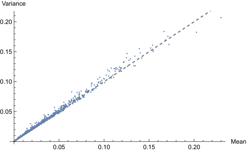
Figure 8. Total number of registered incidents: mean versus variance.

Nevertheless, we observe that there are periods in Figure 7b in which the number of incidents is approximately uniform. Within these periods, the exponential distribution would be a promising fit for the time between two consecutive incident starts. To check if a partition into periods could in fact offer a solution to the observed time-dependence, we identify six periods, as separated by the dashed lines in Figure 7b, in which the number of incidents is roughly uniformly distributed. Modeling the time between two consecutive incident starts on a segment in a single period with an Exponential($\lambda$)-distribution corresponds to a Poisson($\lambda t^{*}$)-distribution for the number of incidents in that period, with $t^{*}$ denoting the period length. Indeed, from Figure 8, which plots, per segment, the mean numbers of registered incidents in an elapsed period against the corresponding variances, we find that the points are concentrated around the $y=x$ line, which is indicative of the Poisson distribution providing a good fit.

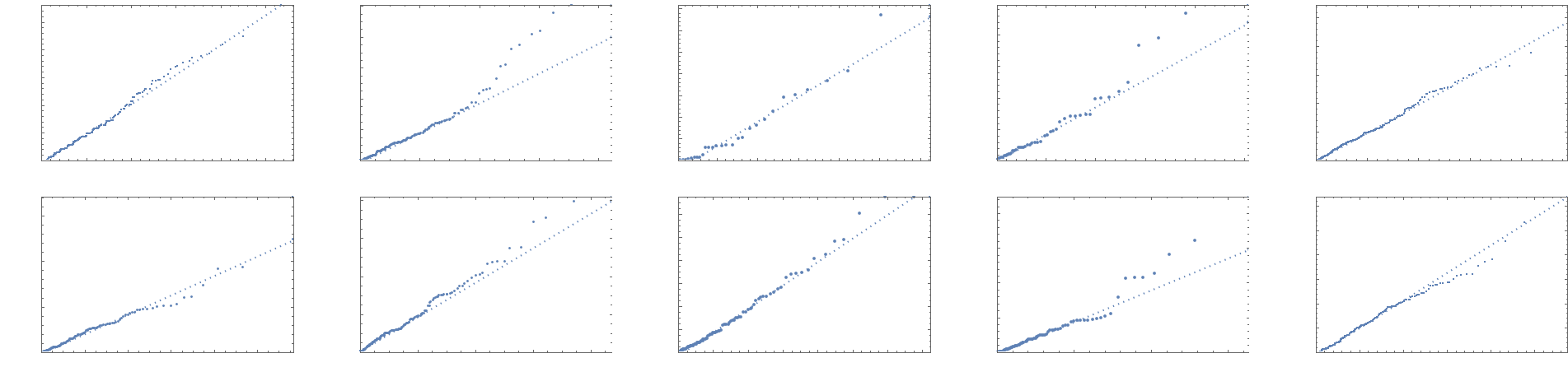
Figure 9. QQ-plots for simulated time between incidents (horizontal axis) against real-world observations (vertical axis). With inter-incident times of high-order, the axes values are omitted for display purposes.

To further assess the quality of the exponential fits over the six periods, we compare simulation results with the rws data. We plot, for ten randomly selected segments, the quantiles of the empirical data distribution of the time between incidents against quantiles of simulations of the time between the start of two consecutive incidents (Figure 9). All QQ-plots show a high degree of linearity between the quantiles, thus corroborating the exponentiality claim. There are some small deviations for large inter-accident times, but we note that these will have little effect on travel time predictions, as travel times generally relate to a considerably smaller timescale.

Two additional remarks on the presented fitting procedure:

• We have identified six periods in which the number of registered incidents behaves roughly uniformly. An even better fit could potentially be obtained by dividing the time-frame into more periods. However, increasing the number of periods will decrease the number of observations per (segment, period)-pair, and may therefore lead to less reliable results. Moreover, a favorable consequence of working with a relatively low number of periods is the resulting low complexity of the resulting mvm.

• Period transitions have been chosen to occur simultaneously at every segment of the network. A potential better fit could be found by adding more detail with a period division per segment, or subset of segments. However, again, the number of observations per segment may limit the quality of these more detailed partitions. Note that the uniform choice in period transitions over all segments also has an advantage when fitting the mvm: we are able to include the duration of these periods in $Y(t)$ (instead of including them in $X_{a_{i}}(t)$ for all $i\leavevmode\nobreak\ =\leavevmode\nobreak\ 1,\dots,n$), which will keep the computational complexity low.

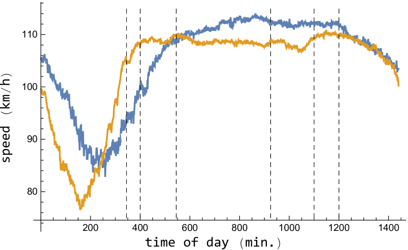
(a) Part of A67 highway.

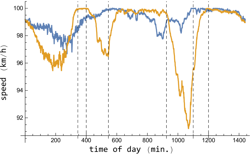
(b) Part of A10 highway

Figure 10. Average maximum speeds at weekends (blue) and weekdays (yellow) in 2017. Vertical lines partition the periods characterized in Section 3.2.

We have established that the time between two incidents in each of the periods in Figure 7b can be modeled by an exponential distribution. For a description of the traffic patterns in this non-incident state, we study the corresponding vehicle speeds. To this end, we have available loop detector data on traffic speeds and traffic flows, provided by ndw. For a given segment, we collect, per minute and per detector located at this segment, the maximum over the registered average speeds of the road lanes. Note that by taking the maximum of the averages we limit the impact of slow-moving vehicles on the collected speed levels. Indeed, we are interested in the per-segment potential driveable speed, which is not well reflected by data corresponding to e.g. trucks. Since the driveable speed cannot exceed the speed limit, we additionally upper bound these maximum average speeds by the speed limit of the corresponding segment.

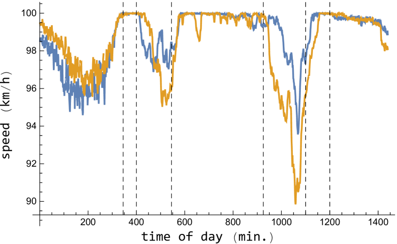
Figure 11. Average maximum speeds on the A10 trajectories at weekdays in February (blue) and May (yellow) in 2017, with rush hour speeds significantly lower for the month May.

For expositional reasons, we present the results of the loop detector data study for two representative highway trajectories: a part of the busy A10 highway around the city of Amsterdam, and a part of the less traveled A67 highway in the southern part of the Netherlands. Figures 10(a) and 10(b) show the average maximum speeds per minute of the day for the A67 and A10 trajectory respectively. From these plots it can be observed that, similar to the duration of the inter-incident state, vehicle speeds are time-dependent. This is most notable in Figure 10(b), in which the speed patterns around the rush hours clearly differ from the patterns outside the rush hours. This time dependence cannot purely be explained by the effect of the time of day, as e.g. the speed patterns during days in the weekend are significantly different from the speed patterns during weekdays. Moreover, besides time of day and day of week, we observe that there are also seasonal effects (Figure 11). Evidently, when estimating travel time distributions, these temporal influences should be taken into account.

When considering the periods as characterized in Figure 7b, there is one period for which the effects of the day of the week and month of the year should play an insignificant role: the night period (8:00pm–6:45am). Since traffic demands in this time interval are typically low, the free-flow speed should always be a good proxy for the mean car speed in non-incident state. However, Figure 10 shows that the attained speed levels during the night are typically low; note that with a relatively high percentage of slow-moving vehicles traveling at night, the resulting imbalanced traffic mix is a probable explanation for this fact. To compare, the mid-day period (09:05am–03:25pm) generally experiences much higher flow levels (Figure 12), but has speed levels that are close to the maximum speed. We therefore conclude that in periods with much lower traffic flows (such as the nights), cars are able to drive at those maximum speeds as well.

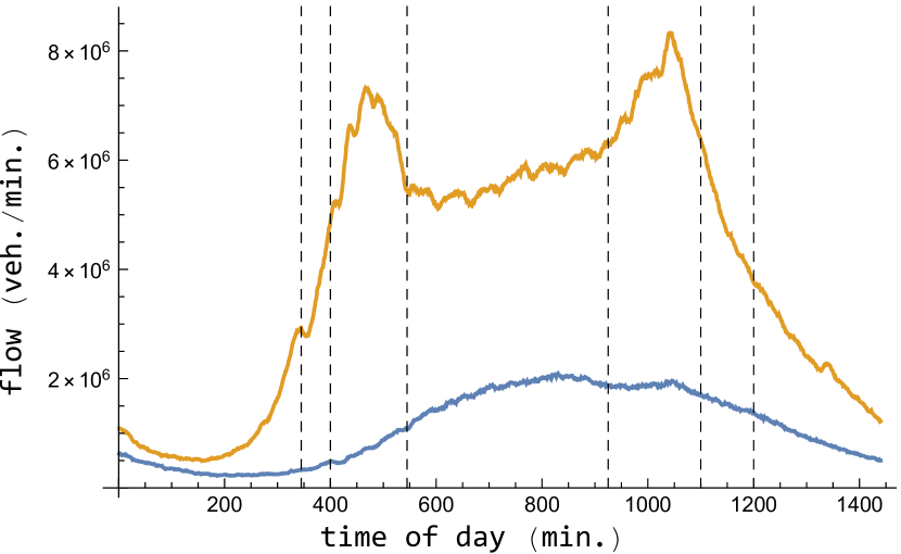
(a) Part of A67 highway.

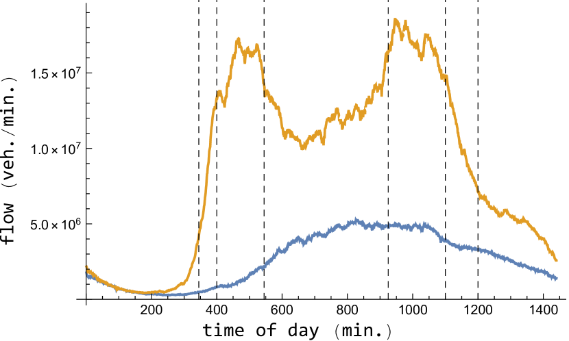
(b) Part of A10 highway.

Figure 12. Average traffic flows on parts of the Dutch highway network at weekends (blue) and weekdays (yellow) in 2017. Vertical lines partition the periods characterized in Section 3.2.

For most segments, speed levels outside the night period are either affected by the day of the week or the month of the year. We will use the velocity data to deduce a few conclusions about the speed patterns in these periods, which will be useful for the prediction of travel time distributions. We focus on the A10 and A67 highway segments of Figure 10, but similar conclusions can be drawn for other highway segments:

• For both highway segments, on weekend days, the highway speed limit is a representative speed level for all six periods. Similar to our reasoning above for the night period, the daily flow levels on these days are typically too low to reduce the driveable vehicle speeds.

• Figure 10(a) shows that on weekdays, the A67 speed levels in the five non-night periods are fairly constant. Indeed, only the first morning rush hour period shows an increasing trend, but the corresponding low traffic flow exposes that, in this period, the actual driveable speeds are close to the speed limit. Therefore, in each of the periods, a constant speed level would serve as good representative for the driveable speed. Note, however, that the appropriate representative speed level may be dependent on the day of the week or the month of the year.

• Figure 10(b) displays that, on a non-weekend day, working with one representative speed level for the A10 segment will certainly work well in the early morning and mid-day periods. The speed patterns in the other periods are not well described by a constant speed level, but do show a distinguishing pattern. That is, around the rush hours, the high traffic flows clearly affect the driveable speeds, showing an approximate V-shape for the speed drops. The period between the evening rush hour and the night period typically serves as recovery period, with decreasing flow levels and, consequently, increasing speed levels.

In conclusion, the speed pattern of a period is generally either well represented by one constant speed level, or captured by (a combination of) decreasing or increasing speed trends. Working with the mvm to model travel time distributions, the speed levels belonging to the different background states need to be chosen such that they emulate these speed patterns.

3.3. Incidents

We continue our analysis by considering incidents. The objectives are in line with those of the inter-incident setting: (i) fit a distribution on the incident duration, and (ii) study the corresponding vehicle speeds. Similar to the inter-incident time, we study incidents per segment, as their duration depends on their location (Figure 13). In the previous subsection, we characterized six periods in Figure 7b in which the number of incidents on a segment is roughly uniform. We will show that, additionally, these six periods suffice to deal with time-dependence in incident length, and describe how to fit a distribution for the incident duration for each (segment, period)-pair.

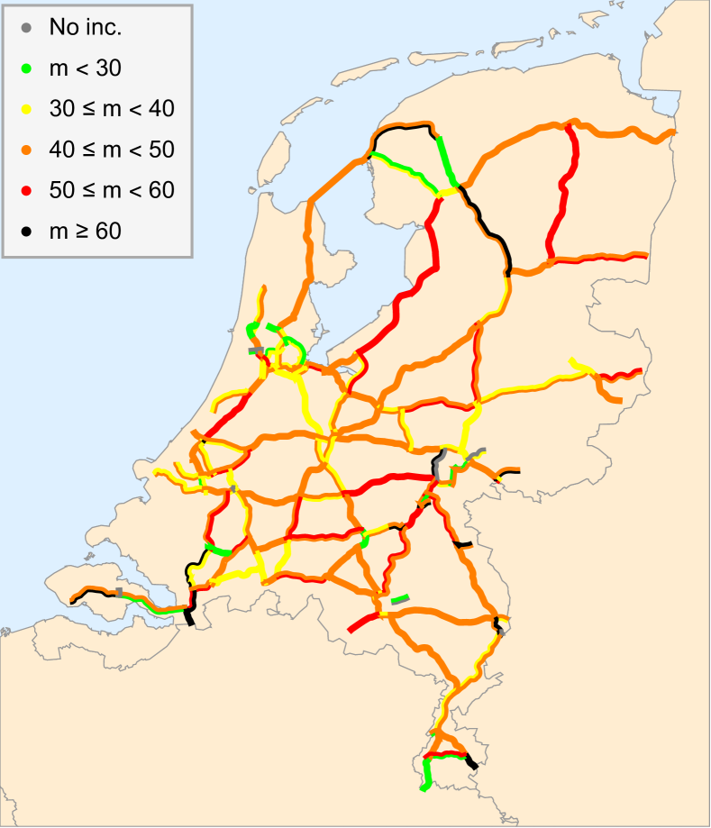
Figure 13. Median incident duration ($m$) per segment (in min.).

First, we observe from Figure 14a that incident length is indeed time-dependent. More specifically, it can e.g. be seen that severe incidents (in terms of duration) occur more frequently within rush hours than outside rush hours. However, for the six periods identified for the inter-incident time, the correlation between the time of occurrence of incidents and their lengths is not significant, as can be seen in Figure 14b. Thus, to describe the incident length on a highway segment, we can fit a distribution for each of these six periods. We are, however, constraint by the amount of data per (segment, period)-pair. Therefore, we further combine periods for which the merged data is still approximately time-independent. As a result, we obtain the three periods (yellow, green, and blue) in Figure 14c, and the objective is to fit a distribution to the incident duration for each of these periods.

To find distributions for the incident lengths, we use the two-moment phase-type matching approximation discussed in Section 2.3. We additionally fit against the Erlang-1 (equivalent to exponential) and Erlang-2 distribution, as these are phase-type distributions with at most the complexity of the hyperexponential and mixture Erlang distribution, making them even more preferable to work with. Initial fits show that outliers have a severe impact on the SCV, and consequently, a negative impact on the fit. Thus, for every data set to fit, the 1$\%$ largest observations are excluded in the computation of the SCV and estimation of the parameters. Importantly, we do include these outliers in the data set when assessing the quality of the obtained fits.

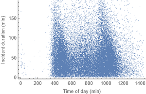
(a) Raw data.

(b) Split into six periods.

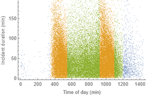
(c) Split into three modes.

Figure 14. Time of day of incident start (in min.) against length of the incident (in min.).

We start the fitting procedure by considering the incident lengths in the night period (Figure 14c, blue). Since, in this period, less than 5% of the segments have more than 15 reported incidents, we merge the observations and fit one distribution that will be used to describe the incident length at night for all segments. With the resulting SCV below 1, this approximating distribution is a mixture of Erlang distributions (see Section 2.3). For the two other periods, we fit an incident duration distribution per (segment, period)-pair, if there are sufficiently many data points for this pair. In case the number of observations in one of the periods is low, but the total number of observations on this segment in the two periods is sufficient, we fit one distribution based on the joint set of observations. For the remaining segments, we merge all observations in the rush hour period (Figure 14c, yellow), as well as in the non-rush hour period (Figure 14c, green), and fit a distribution on both these periods, used for all segments in this category.

	$\%$ rejected	$\%$ non rejected
		Erlang-1	Erlang-2	Hyperexp.	Mixture Erl.
SCV $<1$	$1.1\%$	$1.1\%$	$30.6\%$	-	$68.3\%$
SCV $\geq 1$	$3.3\%$	$68.3\%$	$16.7\%$	$15.0\%$	-

Table 2. Fitting incident lengths for the (segment, period)-pairs. The last four columns show what percentage of the non-rejected fits has the distribution of that column as highest p-value, with p-values obtained through Anderson-Darling tests.

Table 2 shows the results of the fitting procedure. Strikingly, from the 1824 (segment, period)-pairs for which an incident duration distribution needs to be estimated, there are only six pairs for which none of the current fits is accepted. Evidently, we could use more involved methods to find a proper fit for these six pairs. Note that by the denseness of the class of phase-type distributions (Asmussen, 2003, Section III.4), we can include these into our Markovian framework as well.

Remark 2.

In the above, we fit the distribution of incidents based on their location and period of occurrence. In case there is currently an incident in the network, there is often additional information available, e.g. regarding the nature of the incident, the involvement of trucks, etc. Importantly, the presented fitting procedure is very flexible, and can take this information into account. That is, we may limit the data used to fit such that the considered instances correspond with the current incident conditions. For example, if it is known that there is currently a vehicle breakdown, we may fit the distribution of the (residual) duration of this incident on the subset of all incident data entries occurred on the same segment, having vehicle breakdown as registered cause. $\Diamond$

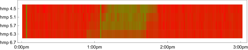
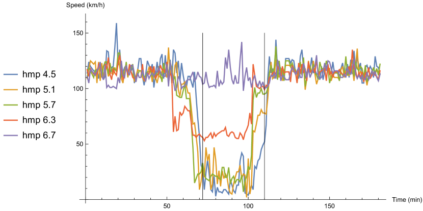
(d) Heat map.

(e) Line plot.

Figure 15. Maximum speeds as registered by five detectors around an incident on 16-04-2017 at highway A10. The left time point in both plots corresponds to midnight. The detectors are identified by the signalling hectometre indication closest to their location, with the indications being hectometer poles (hmp), standing 100 metres apart through the highway network.

We proceed by investigating the speed patterns around the reported incidents, such that we are able to model the impact of incidents on the driveable vehicle speeds. Importantly, we will argue that, during an incident, the vehicle speeds on surrounding highway parts are generally well captured by one constant speed level, whose value depends on the distance of the highway part to the location of the incident. Naturally, this dependence is only local, and thus, for highway parts located far from the incident, the driveable vehicle speed is not affected by the incident.

Incidents are likely to lead to a substantial reduction of the driveable speed, an example of which is given in Figure 15. Note that, similar to the procedure for the non-incident speeds, we show the maximum of the average driven speeds over the road lanes, as this best reflects the driveable car speed. Now, we observe that for the longest part of the incident depicted in Figure 15, the speed levels at the individual detectors are relatively stable. Indeed, with the two vertical lines indicating the reported start and end time of the incident, we observe that, with exception of the short periods during the start and end of the incident, the vehicle speeds per detector fluctuate around a single speed level. Thus, around every detector, the driveable speed pattern during the studied incident could roughly be summarized by one speed value. Using harmonic averaging, a representable incident speed level for a slightly larger highway part, containing multiple detectors, can be found.

Figure 15 also shows the spatio-temporal effect of traffic jams: the incident affects the velocities at detectors with a further upstream distance from the incident location typically somewhat later and considerably less severe (in terms of the speed drop value). Indeed, it can be observed that the speed level at the detector around hectometer pole (hmp) 6.3 is only slightly affected by the incident, whereas the speed level at the detector around hmp 6.7 is the same before, during, and after the incident. Generally, an incident only affects the speeds at highway parts relatively close to the incident location. By studying historical speed patterns of incidents, we can deduce the area that is potentially affected by an incident located at a given highway part.

In the above, we only showed the speed pattern during the incident depicted in Figure 15. However, the relatively low speed fluctuation during the largest part of the incident does not only show for this incident, but is a more observed phenomenon across the studied incidents in the Dutch highway network. Thus, we claim that, for every highway part located around an incident, the driveable speed is well described by just one speed level. Moreover, conform the speed patterns in Figure 15, typically, the highway parts that are not located around an incident in the network, do not suffer a speed drop during the incident.

Now, recognizing the frequently observed stability of speed patterns during incidents, when working with the mvm to model travel time distributions, we can, for a given incident, simply use one speed level per highway link for all background states encoding this incident. Note that the observation of low incident speed fluctuation is particularly useful in the case the incident is present at the vehicle’s departure. Indeed, in this case, the corresponding incident speed levels can directly be estimated by the collected speeds in the minutes prior to the departure.

4. Operationalizing the Markovian velocity model

Considering a vehicle that plans to traverse a given path between an origin and a destination in the Dutch highway network, at a specific day and time, this section demonstrates how to employ the mvm to obtain the corresponding travel time distribution. The approach followed incorporates the effects of events that directly impact the driveable speeds. We consider the situation that (i) the analysis discussed in Section 3 has been performed, (ii) the network state corresponding to the vehicle’s departure is known (in terms of the location and starting time of current incidents), and (iii) information regarding existing or upcoming scheduled events (e.g. road work, bad weather conditions) is available.

Recall that the mvm models the events affecting arc speeds through an environmental background process $B(t)$. Section 4.1 details how to construct this background process $B(t)$, so as to incorporate the recurrent and non-recurrent events potentially affecting the departing vehicle’s trip time, and Section 4.2 discusses how to set the driveable speed levels corresponding to the different states of $B(t)$.

4.1. Background process

With $n=1378$ directed links in the Dutch highway network, the background process of the mvm takes the form $B(t)=(Y(t),X_{1}(t),\ldots,X_{n}(t))$. Here, $X_{i}(t)$ models the occurrence of incidents on link $i$, and $Y(t)$ the (semi-)predictable events. Concretely, $Y(t)$ captures the recurrent, daily patterns with a Markov process $Y_{0}(t)$, and the scheduled events upon the vehicle’s departure with Markov processes $Y_{1}(t),\dots,Y_{m}(t)$ (in case there are $m$ such events). Importantly, with incident characteristics e.g. dependent on the time of day, the Markov link processes $X_{i}(t)$ are dependent on the state of the common process $Y(t)$.

4.1.1. Daily patterns

Since the different traffic regimes during the day are roughly described by the in Figure 7b identified periods, $Y_{0}(t)$ captures the daily, recurrent traffic patterns by modeling the durations of these six periods. Observe that the durations of these periods are quite predictable. Notably, including events whose durations have little variability can be achieved by modeling these durations with Erlang phases. Concretely, for given $k\in\mathbb{N},t\in\mathbb{R}_{>0}$ and $Z_{1},\dots,Z_{k}$ i.i.d. exponentially distributed random variables with mean $t/k$, we have that $\sum_{i=1}^{k}Z_{i}$ is Erlang($k,k/t)$ distributed, such that

$$\mathbb{E}\Big{[}\sum_{i=1}^{k}Z_{i}\Big{]}=t,\quad\quad\quad\text{Var}\Big{[}\sum_{i=1}^{k}Z_{i}\Big{]}=t^{2}/k.$$

Thus, modeling predictable events with a given mean by an Erlang-$k$ distribution with the same mean, we obtain a suitably low variance when choosing $k$ sufficiently large.

Given the departure time of the vehicle, we know the remaining time of the current period, denoted by $t_{0}$, as well as the lengths of the subsequent periods, denoted $t_{1},t_{2},\ldots,t_{6}$. Now, in case duration $t_{i}$ is modeled with $k_{i}$ Erlang phases, the process $Y_{0}(t)$ in principle has a total of as many as $k_{0}+\dots+k_{6}$ states. Fortunately, travel times are typically in the order of minutes up to hours, so that a trip will overlap with a low number of periods. This concretely means that we only need to include into $Y_{0}(t)$ the phases corresponding to these periods. Hence, with $M$ a crude upper bound for the time the vehicle arrives at its destination, we may omit all states belonging to periods that are extremely unlikely to be entered before time $M$. An example of a resulting structure of $Y_{0}(t)$ is given in Figure 16, only containing states belonging to either of the first two periods.

Figure 16. Example structure $Y_{0}(t)$.

(a) Duration of an existing event modeled by an Erlang($k,k/t^{\prime}$)-distribution.

(b) Time until and duration of a predicted event modeled by an Erlang($k_{1},k_{1}/t^{\prime}_{1}$) and Erlang($k_{2},k_{2}/t^{\prime}_{2}$)-distribution respectively.

Figure 17. Example structures scheduled events $Y_{1}(t),\dots,Y_{m}(t)$.

We claim that using just a few phases per period (e.g. , $k_{i}\in\{5,\ldots,10\}$) is already sufficient to model the period lengths well. The reason is that such a choice of $k_{i}$ already reduces the variance of the time spent in period $i$ with a factor between 5 and 10 compared to the exponential distribution. It is also noted that working with larger $k_{i}$ values would ignore the intrinsic fluctuations of the periods’ start and end times. Moreover, working with large values of $k_{i}$ has the undesired consequence of inflating the state space of $B(t)$, thus leading to a high computational complexity.

4.1.2. Scheduled events

We can use the same ideas to capture the duration of the $m$ scheduled events that are modeled through the processes $Y_{1}(t),\dots,Y_{m}(t)$. That is, if event $i$ is an existing event (i.e., present at the vehicle’s departure) for which the expected remaining duration is known to equal $t^{\prime}$, we can use the Erlang($k,k/t^{\prime}$)-distribution to model the duration of event $i$ (Figure 17(a)). In case event $i$ is not an existing but a forecasted event, $Y_{i}(t)$ should, besides the duration of the event, also include Erlang phases that model the time until the start of the event (Figure 17(b)).

Remark 3.

If, besides information on the mean duration of a scheduled event (or the time until its start), there is information available on the variance of the duration (or the time until its start), one can alternatively fit its distribution with the two-moment phase-type matching techniques that were presented in Section 3.3. $\Diamond$

4.1.3. Incidents

With the general structure of $Y(t)$ known, we are now able to characterize the Markov processes $X_{1}(t),\dots,X_{n}(t)$, that model the incidents on the links of the network, conditional on the state of $Y(t)$. Concretely, we let the dynamics of $X_{i}(t)$ depend on the state of $Y_{0}(t)$, since it was concluded in Section 3 that incident dynamics depend on the specific period of the day. Note that these incident dynamics should cover the incident duration itself, as well as the inter-incident time. Recall that in Section 3, these distributions are fitted per highway segment (i.e., highway part between two highway intersections), whereas $X_{i}(t)$ should capture these distributions per highway link (i.e., highway part between two ramps).

Given the period of the day, encoded by the state the process $Y_{0}(t)$ is in, we have shown in Section 3.2 that, for every highway segment, the time between two incidents in this period can be modeled by an exponential distribution. We will now argue that the inter-incident duration on the links that partition this segment can be described by the exponential distribution as well. This implies that, for a link $i$, the process $X_{i}(t)$ contains just one exponential state that represents the situation in which the link is incident-free. The mean time spent in this state depends on the period of the day, i.e., on the state of $Y_{0}(t)$.

Denote by $1/\lambda_{j,k}$ the mean inter-incident time on segment $j$ in case $Y_{0}(t)=k$ (i.e., $\lambda_{j,k}$ is the rate of the corresponding exponential distribution). To see that the inter-incident distribution of the links that partition this segment is indeed exponential, note that the initiation of an incident on segment $j$ corresponds to the initiation of an incident on one of these links. Therefore, we assign a value $p_{i}^{j}\in[0,1]$ to every link $i$ on segment $j$, representing the probability that, given there is an incident on segment $j$, this incident has occurred at link $i$. As a natural proxy for $p_{i}^{j}$ we take the ratio of the lengths of link $i$ and segment $j$. Observe that, in modeling terms, the inter-incident time on link $i$ will have an Exponential($p_{i}^{j}\lambda_{j,k}$)-distribution. Importantly, since the inter-incident time on segment $j$ is the minimum of the inter-incident times on the links at $j$, we (consistently) obtain the Exponential($\lambda_{j,k}$)-distribution for the inter-incident time on the full segment.

If, for link $i$, the process $X_{i}(t)$ transitions out of the inter-incident state, this corresponds to the occurrence of an incident on this link. As was concluded in Section 3.3, the distribution of the duration of such an incident depends on the period of the day in which the incident occurs. Therefore, for every period modeled by $Y_{0}(t)$, the process $X_{i}(t)$ should contain states that describe the duration of an incident which started in that period. For example, in case $Y_{0}(t)$ is structured as in Figure 16, $X_{i}(t)$ contains states that describe an incident which started in the period modeled by $k_{0}$ phases, as well as states that describe an incident which started in the period modeled by $k_{1}$ phases.

Given the period that corresponds to the state of $Y_{0}(t)$, we have fitted the distribution of the duration of an incident starting in this period for every highway segment in the Dutch network (Section 3.3). Now, given such a segment, we will use the corresponding incident distribution for every link that partitions this segment. Thus, if a highway segment between two intersections consists of three links, separated by ramps, the incident distribution that was fitted for the segment is used to model incidents on all these three links. Recall that, because the fitted distributions all fall in the category of phase-type distributions, we can directly include these in the Markov processes $X_{i}(t)$.

A special case are the incidents that are already present upon the vehicle’s departure. Given that link $i$ has an incident, knowledge of the starting time of the incident yields both the distribution of the incident length and the current running time of the incident, from which we can deduct the distribution of the remaining incident length. Then, the process $X_{i}(t)$ should also include states modeling this remaining incident length, which $X_{i}(t)$ visits before transitioning to the inter-incident state. Trivially, if the incident distribution is exponential, the remaining incident time is also exponentially distributed. For an incident with current running time $t>0$ and hyperexponentially distributed length with parameters $p\in[0,1],\mu_{1},\mu_{2}\in\mathbb{R}_{>0}$, we have:

$$\mathbb{P}(X\!>\!t\!+\!s\,|\,X\!>\!t)=\frac{\mathbb{P}(X\!>\!t\!+\!s)}{\mathbb{P}(X\!>\!t)}=\frac{pe^{-\mu_{1}(t+s)}+(1\!-\!p)e^{-\mu_{2}(t+s)}}{pe^{-\mu_{1}t}+(1\!-\!p)e^{-\mu_{2}t}}=qe^{-\mu_{1}s}+(1\!-\!q)e^{-\mu_{2}s},$$

with

$$q:=\frac{pe^{-\mu_{1}t}}{pe^{-\mu_{1}t}+(1\!-\!p)e^{-\mu_{2}t}}.$$

Thus, the remaining incident time has a hyperexponential distribution as well, with parameters $q,\mu_{1},\mu_{2}$. It can be proven that the distribution of an Erlang$(k,\mu)$ random variable, conditioned on being at least $t$, is a mixture of Erlang$(j,\mu)$ distributions, with $j=1,\dots,k$ (Theorem 1, Appendix A). This gives that the remaining time of an Erlang-2 distribution can be cast in the Markovian framework. Moreover, it can now easily be deduced that the remaining incident time of a mixture Erlang distribution is a mixture Erlang distribution as well.

4.2. Speed levels

To obtain the travel time distribution for the vehicle, the speed levels corresponding to the different background states have to be specified. That is, for all $i$ and all $s\in S$, we need to set a value for $v_{a_{i}}(s)$, the speed at which vehicles are moving on link $a_{i}$ given $B(t)=s$. Without loss of generality, we focus on the speed levels of link $a_{1}$. Recall from Section 3.3 that, with incidents being local events, only incidents on links surrounding $a_{1}$ will affect the speed on this link. Denote this set of links whose congestion status affects $a_{1}$ by $A_{a_{1}}$.

Let $s\in S$ be a state that corresponds to a setting in which the arcs in $A_{a_{1}}$ are incident-free, and there are no existing scheduled events in the network. Then, the driveable speed on $a_{1}$ is fully determined by the daily velocity patterns. The speed and flow data analysis as performed in Section 3.2 has revealed during which periods, and thus for which states of $Y_{0}(t)$, the driveable speed level on $a_{1}$ equals the free-flow speed. In case the state of $Y_{0}(t)$ belongs to a non free-flow (but still relatively constant) speed period, historical averaging of the maximum of the road lane speeds yields a representative speed level per loop detector on link $a_{1}$. For this averaging, we only use speed data of the days of the week that match the current day, and only from a few weeks preceding the vehicle’s departure. This way, we account not only for within-day time-dependence, but for dependence on the day of the week and season as well. Now, to obtain a representative speed level for the complete link, we simply take the weighted harmonic mean of the speeds levels of the individual detectors located on the link. The weights are set to account for the non-uniform placement of the loops on the link, the weight of a single detector being the total distance between the midway points to its neighbors, or, in case of only one neighbor, the distance from this one midway point to the boundary of the link.

Importantly, we can easily work with more elaborate speed patterns, in case one constant speed level is not representative for the speed pattern in the considered period. That is, by assigning different speed levels to the different Erlang phases that model the duration of this period, the driveable speed (as function of time) is a step function. Being able to model stepwise speed functions allows to replicate more complex daily patterns, such as the observed V-shape during the rush hour on the A10 (Figure 10(b)). The numerical examples in Section 5 will indeed reveal that it is not always necessary to replicate these shapes perfectly, and that, for the considered instances, working with step functions is already satisfactory.

Now, let $s\in S$ be a state that corresponds to a setting in which one of the arcs in $A_{a_{1}}$ is not incident-free. As argued in Section 3.3, during this incident, the driveable speed on link $a_{1}$ can roughly be described by one speed level. In case the incident is already present upon the vehicle’s departure, real-time information regarding the driven speeds at the detectors on $a_{1}$ may be available. If these reveal that the incident is in a stationary state, i.e., speed fluctuations in the minutes prior to the departure are only mild, we can set the speed level on $a_{1}$ in state $s$ as the current speed level on $a_{1}$. Alternatively, if the last minutes of speed data do not show a somewhat stable pattern, the link speed that corresponds to the last minute of data is set as speed level for $s\in S$. In case the incident has just started or is in the process of clearance, typically corresponding with respectively a decreasing or increasing speed trend, this estimate is expected to be a better representative than an average over a longer period.

In case there is no real-time speed data available, or the incident is not already present at the vehicle’s departure, the speed level of the incident is unknown, and estimated by the average of the historical speed levels of incidents located on the same link. To obtain the stable speed level of a historical incident, we propose to take, as above, the weighted harmonic average of the stable speed patterns of the individual loop detectors. For every such detector, the stable speed level is identified by computing, for every ten minutes of data around the time interval of the incident, the mean and variance in registered speeds. Then, from all means below 80 km/h, the stable speed level is set as the one with the minimum variance. Figure 18 shows the result for two historical incidents on the highway A10.

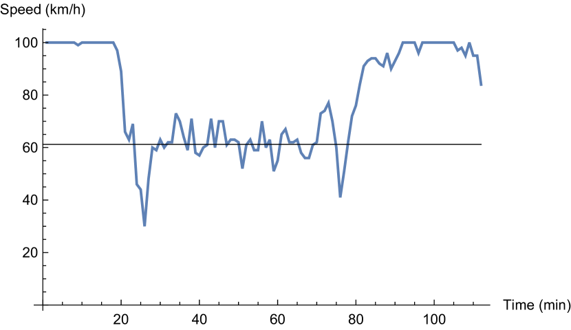
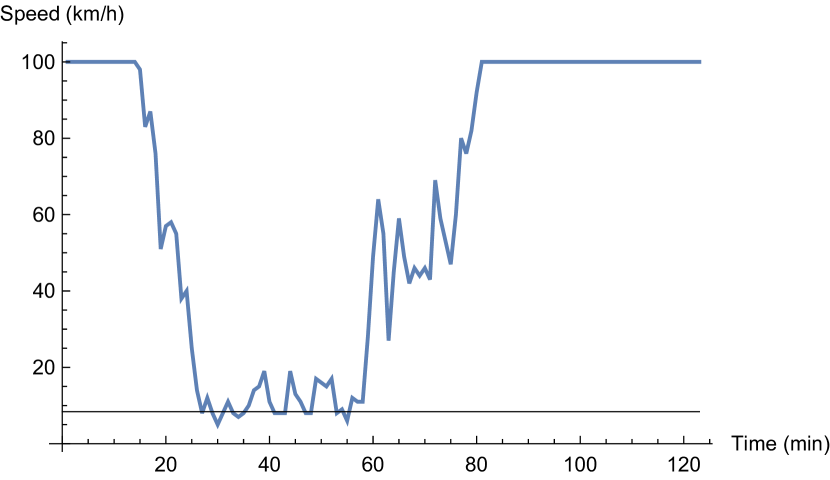
Figure 18. Identifying the stationary speed level of two historical incidents.

Evidently, in case there are multiple incidents in the vicinity of arc $a_{1}$, the speed on $a_{1}$ is at least as much affected as it would be by one of these individual incidents. Therefore, for $s\in S$ for which there are multiple arcs in $A_{a_{1}}$ that have incidents, we simply set the velocity on $a_{1}$ in state $s$ as the minimum of the speed levels of $a_{1}$ corresponding to the individual incidents.

In case there are existing or upcoming scheduled events modeled through $Y(t)$ (e.g. road work or bad weather), the effect of these events should be taken into account as well. The speed levels on the arcs affected by the scheduled events are estimated in a similar way as the incident speeds. That is, if the event is present at the vehicle’s departure and current speeds are available, these speeds are used to estimate the presentable speed level. If these speeds are not available, or the event is a future event, historical speed data is used to determine the correct speed level.

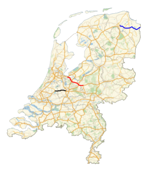
Figure 19. Three considered paths in the Dutch highway network.

5. Numerical experiments

Having described and substantiated the individual components of our procedure, we will now display the resulting travel time distributions for several case studies and provide examples of the advantage of our model as compared to traditional travel time estimation methods. The case studies consider the traversal of three west-to-east directed paths in the Dutch highway network, depicted in Figure 19, under various traffic scenarios. Concretely, for each of these paths, we look at the travel time distribution of vehicles traversing the path in the non-rush hour and rush hour setting, in case the path is incident-free upon departure (Section 5.1). Additionally, in Section 5.2, we consider a traffic setting where, upon the vehicle’s departure, there is an incident on the path to travel. With the time until clearance of the incident a random variable, our procedures, taking this uncertainty into account, are shown to outperform deterministic estimations.

Before doing so, we briefly explain why the available travel time data was not adequate for a more detailed (numerical) assessment of the performance of our methodology. That is, naturally, one would want to compare the travel time distributions we obtain for the traversal of the three paths under various traffic settings with travel time data from the Dutch highway network. However, hampered by the availability and quality of the travel time data as provided by ndw, such a comparison could not be performed.

Limitations arise due to the fact that, with poor availability of both floating car data and travel time data collected via Bluetooth or cameras (for the years of study), the ndw data only contains rough, rounded estimates of average travel times, based on measurements with loop detectors. In fact, per trajectory and per minute, there is only one ndw data value that represents the general mean travel time, averaged over all vehicles (cars and trucks) on the segment under consideration. Since the maximum speed trucks are allowed to drive in The Netherlands is lower than the maximum car speed, a comparison would (incorrectly) lead to the conclusion that our travel-time estimates are too low. Indeed, with traffic heterogeneity playing a prominent role, the realized speed levels are typically below the actual driveable speeds, limiting a fair numerical comparative analysis. A second conceptual complication is that our procedures are based on capturing the travel times that vehicles are effectively able to drive, in contrast to the collected travel time data, which only reflects (rough estimates of) realized travel times, which are subject to the heterogeneity in driving style of individual vehicles.

5.1. Travel time distributions under the absence of incidents

Focusing on the travel time distributions on the three paths of Figure 19, it is important to note that the paths are of a different characteristic nature. For example, they differ greatly in terms of incident-proneness, as can be observed from Figure 7. For the blue path, which is approximately 37 km long and located in a rural area, the mean inter-incident time is highest. The red path, which is approximately 30 km long and brings vehicles from the city of Amsterdam to a more rural area, has a relatively low mean inter-incident time. The mean time between incidents is lowest for the circa 38 km long black path between two busy urban areas.

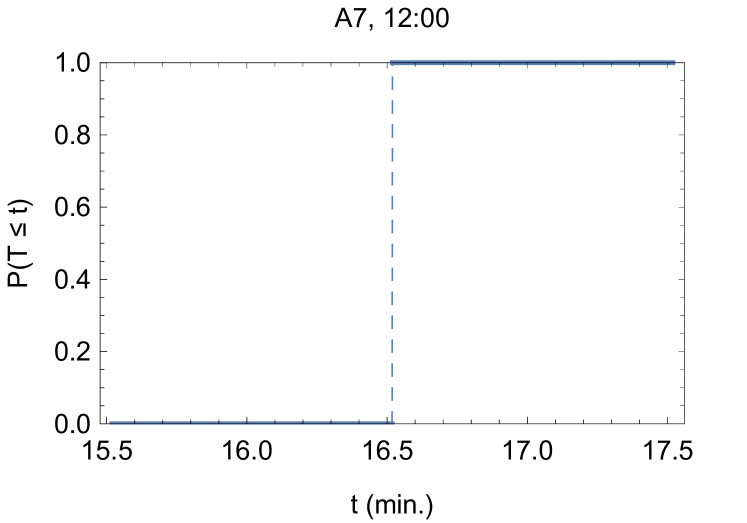
(a) A7

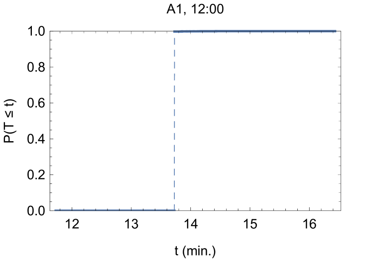
(b) A1

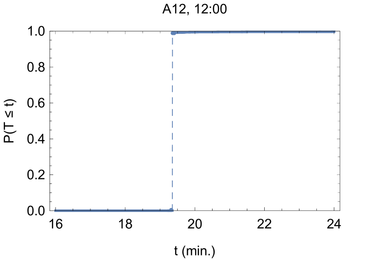
(c) A12

Figure 20. Cumulative travel time distribution estimates for departure at a regular Wednesday at noon in 2019.

We first consider the traversal of the paths in an incident-free non-rush hour setting. Specifically, we look at vehicles traveling the paths on a regular Wednesday (i.e., no school holiday or national holiday) in the year 2019 at noon, in case there are no registered incidents upon departure. In accordance with Section 4, the speed levels in the non-incident setting are estimated by averaging over the speeds of the four regular and incident-free Wednesdays prior to the considered day, and the speed levels of future incidents are estimated by averaging speed levels of historical incidents on the same highway link. The resulting cumulative travel-time distributions are presented in Figure 20. Recall that our model does not take into account fluctuations that typically arise due to the differences in driving styles, which explains the nearly deterministic pattern. Indeed, since both the probability of incident occurrence during the trip and the probability of hitting the next time period, corresponding to rush hour conditions, are extremely small, the driveable vehicle speed during the trip is well described by one constant velocity level.

Now, let us alternatively consider a vehicle that departs at a regular 2019 Tuesday at 3:15 p.m. or 6:00 p.m. At the first time instant, upon the vehicle’s departure, the onset of rush hour is in the near future, whereas the second departure instant falls within the rush hour period. In contrast to the non-rush hour setting, the travel time distributions at these instances, as displayed in Figure 21, clearly show the different characteristic natures of the considered paths. That is, with low daily flow levels in all periods, the driveable speed levels on the A7 highway equal the free flow speed, again leading to an approximately deterministic distribution, independent of the departure time. On the other hand, the A1 and A12 highway do show uncertainty. For departure at 3:15 p.m., this uncertainty is only mild, as a large part of the paths is traversed in non-rush hour setting, which knows constant traffic speeds. However, the width of the travel time distributions is larger for departure at 6:00 p.m., with the travel times suffering from the (semi-)random onset of the different rush-hour speed trends.

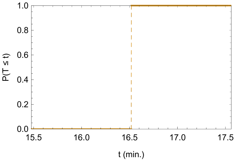
(a) A7

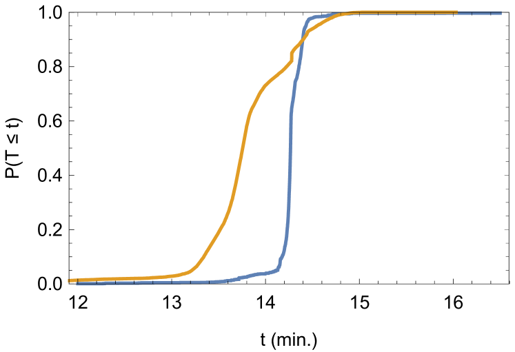
(b) A1

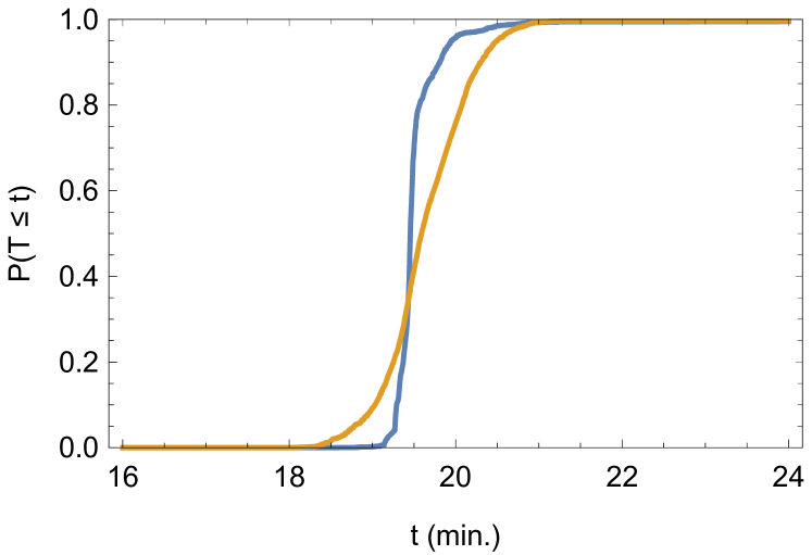
(c) A12

Figure 21. Cumulative travel time distribution estimates for departure at Tuesday 3:15 p.m. (blue) and 6:00 p.m. (yellow) in 2019.

5.2. Travel time distributions under the presence of incidents

Due to the relatively high amount of uncertainty, the most interesting distribution estimates arise in case, upon the vehicle’s departure, there is an incident on the path to travel. In such traffic scenarios, our procedures are clearly beneficial over traditional, deterministic methods that either restrict to working with current speeds or only take recurrent patterns into account. That is, these are unable to work with random future changes in traffic conditions, yielding poor travel time estimations in case there is a high probability of such changes. For example, traditional methods are often insufficient when the incident is located at the end of the path to travel, since, with relatively much time until the vehicle reaches the incident location, there is typically a high probability of incident clearance before reaching the incident. Another example in which current route-planners may perform unsatisfactorily is presented in Figure 22, which shows the cumulative travel-time distributions for a specific incident, a defective truck at the first part of the A1 path, when departing after 25%, 50% or 75% of the total reported incident duration.

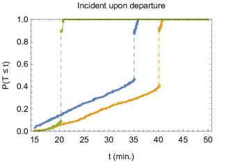
Figure 22. Travel time distribution when traversing the A1 path in incident setting. Departure time is after $25\%$ (blue), $50\%$ (yellow) or $75\%$ (green) of the total incident duration.

To illustrate how the MVM can be used to improve routing advice, we first consider a vehicle departing at the 25% time instant. Obviously, the remaining incident duration is unknown to the driver itself. With traditional methods not accounting for random changes, route planners will predict a travel time of 35.1 minutes, i.e., the travel time that corresponds to the location of the probability mass point of the 25% distribution. Indeed, observe that the mass point corresponds to the scenario in which the considered incident is not cleared during the traversal of the links affected by this incident. In contrast, our method does take into account that with a certain probability, the incident will have cleared before the vehicle arrives at the congested links. On the A1 path, there is a high percentage of reported incidents with relatively short duration. Thus, the distribution of the remaining incident duration has high probability mass on the left side, yielding a high probability of clearance before reaching the incident. The mass point of the obtained distribution indeed reveals that there is an almost 40% chance that the incident has cleared before the vehicle arrives. Therefore, in expectation, the travel time will be significantly less than the 35.1 minutes estimated by traditional route-planners.

In the case where 50% percent of the incident duration has elapsed upon departure, it can be observed from Figure 22 that our procedure estimates that there is a high probability that the incident is cleared during the traversal of the path, yielding, again, an expected travel time that is significantly less than the 40.1 minutes that will be estimated by traditional methods. Note that, as the position of the mass point provides an impression for the incident speed levels, the driveable incident speeds are lower than those recorded after 25% of the incident. This can be explained by the fact that, after 25% of the total incident duration, the speed levels at detectors further away from the incident may not be affected yet, since the traffic jam is still accumulating, leading to slightly lower travel time values when compared to the 50% scenario.

When departing after 75% of the incident duration, the mean travel time estimate of the mvm is almost the same as when using a deterministic method: they would both yield an estimate of 20.3 minutes. This is inherent to the small probability that the incident is cleared during traversal of the path. Observe, moreover, that the location of the mass point indicates that, compared to departure after 25% and 50% of the incident duration, the speeds are significantly closer to their non-incident version. Reviewing the incident characteristics, it is revealed that this is due to the fact that the lanes that were closed at the 25% and 50% instances, are fully opened after 75%, with recovery speeds shortly revealing a shockwave pattern.

6. Conclusive remarks

In this paper we presented comprehensive techniques to describe the randomness of incidents in a highway network, in terms of their frequency, duration and impact on vehicle speeds. With these results, we were able to operationalize the Markovian velocity model, a stochastic model that tracks both recurrent and non-recurrent traffic events that affect driveable vehicle speeds. Numerical experiments demonstrated the impact of recurrent and non-recurrent effects on such travel time distribution estimates in various traffic settings.

We have shown that, on a given highway segment, both the incident duration and inter-incident time are dependent on the time of day, but that we can deal with this time-dependence by working with periods in which these effects are essentially constant. For every highway segment, the inter-incident time within each of these periods is well described by an exponential distribution, whereas, in nearly all cases, the duration of an incident starting in this period fits a phase-type distribution with a relatively low number of phases. When fitting the incident data, we have used the collection of all registered incidents per highway segment, and not distinguished on environmental conditions. A future study could include both incident and weather data, and investigate the impact of different weather conditions on the incident length and driveable vehicle speeds. This could further improve the prediction results in case, upon the vehicle’s departure, weather conditions are poor.

To operationalize the Markovian velocity model, we presented methods to obtain representative levels for the driveable vehicle speeds in both the incident and inter-incident setting. In the inter-incident setting, it could be observed that these speed levels depend on the period-of-day, day-of-week and time-of-year. To tackle these dependencies, we proposed a simple, fast and transparent clustering method, in which we just average over the speeds observed in the same period and on the same day, in the weeks previous to the vehicle’s departure. Evidently, more enhanced prediction methods could be used to find representative speed levels.

The numerical experiments we conducted showed the impact of recurrent traffic patterns, current incidents and potential future incidents on the travel time distribution estimates. It was observed that the impact of future incidents is minor, whereas the impact of both rush hour and current incidents is more pronounced. Future work could be specified towards incorporating the impact of second-order effects into the travel time distribution estimates as well. A potential suggestion would be to incorporate the heterogeneity in driving by style by letting the vehicle speeds – instead of being constant – be described by a distribution that depends on the state of the background process.

As discussed in Section 5, the absence of reliable travel time data prohibits a full comparison between the obtained travel times estimates and real-world data. However, we have been able to show the advantages compared to traditional travel-time prediction methods through some illustrative examples. A more extensive comparison is clearly desirable, and should be carried out once there is access to more suitable travel time data. Note that, with current technical advances, floating car data is expected to become available on a large scale in the upcoming years.

Appendix A Conditional Erlang distribution

Theorem 1.

For $t\in\mathbb{R}_{>0}$ and $X\sim\text{Erlang}(k,\mu)$, the distribution of $X\,|\,X\!>\!t$ is a mixture of Erlang$(j,\mu)$ distributions with $j=1,\dots,k$.

Proof.

For an Erlang$(k,\mu)$ distribution we have:

$$\tilde{p}(t):=\mathbb{P}(X>t)=\sum_{n=0}^{k\!-\!1}\frac{e^{-\mu t}}{n!}(\mu t)^{n}.$$

Thus, Newton’s Binomium gives that:

$$\mathbb{P}(X\!>\!t\!+\!s\,|\,X\!>\!t) =\frac{1}{\tilde{p}(t)}\sum_{n=0}^{k-1}\frac{e^{-\mu(t+s)}}{n!}(\mu(t\!+\!s))^{n}=\frac{1}{\tilde{p}(t)}\sum_{n=0}^{k\!-\!1}\sum_{j=0}^{n}\frac{e^{-\mu(t+s)}}{j!(n\!-\!j)!}(\mu t)^{j}(\mu s)^{n-j}$$

$$=\frac{1}{\tilde{p}(t)}\sum_{j=0}^{k-1}\sum_{n=j}^{k-1}\frac{e^{-\mu(t+s)}}{j!(n\!-\!j)!}(\mu t)^{j}(\mu s)^{n-j}=\frac{1}{\tilde{p}(t)}\sum_{j=0}^{k-1}\frac{e^{-\mu t}}{j!}(\mu t)^{j}\sum_{n=0}^{k\!-\!1\!-\!j}\frac{e^{-\mu s}}{n!}(\mu s)^{n}$$

$$=\frac{1}{\tilde{p}(t)}\sum_{j=0}^{k-1}\frac{e^{-\mu t}}{(k\!-\!1\!-\!j)!}(\mu t)^{k-1-j}\sum_{n=0}^{j}\frac{e^{-\mu s}}{n!}(\mu s)^{n}=\sum_{j=1}^{k}\tilde{p}_{j}(t)\sum_{n=0}^{j-1}\frac{e^{-\mu s}}{n!}(\mu s)^{n},$$

with

$$\tilde{p}_{j}(t):=\frac{1}{\tilde{p}(t)}\frac{e^{-\mu t}}{(k\!-\!j)!}(\mu t)^{k-j}.$$

We conclude that the remaining time of an Erlang$(k,\mu)$ random variable, conditioned on being at least $t$, is a mixture of Erlang$(j,\mu)$ distributions with $j=1,\dots,k$; with probability $\tilde{p}_{j}(t)$ there are $j$ phases. Indeed,

$$\sum_{j=1}^{k}\tilde{p}_{j}(t)=\frac{1}{\tilde{p}(t)}\sum_{j=1}^{k}\frac{e^{-\mu t}}{(k\!-\!j)!}(\mu t)^{k-j}=\frac{1}{\tilde{p}(t)}\sum_{j=0}^{k-1}\frac{e^{-\mu t}}{(k\!-\!j\!-\!1)!}(\mu t)^{k-j-1}=\frac{1}{\tilde{p}(t)}\sum_{j=0}^{k-1}\frac{e^{-\mu t}}{j!}(\mu t)^{j}=1.$$

∎

References

- (1)
- Asmussen (2003) Asmussen, S. (2003), Applied Probability and Queues, second edn, Springer New York.
- Bergel-Hayat et al. (2013) Bergel-Hayat, R., Debbarh, M., Antoniou, C. and Yannis, G. (2013), ‘Explaining the road accident risk: Weather effects’, Accident Analysis & Prevention 60, 456–465.
- Chalumuri and Yasuo (2014) Chalumuri, R. S. and Yasuo, A. (2014), ‘Modelling travel time distribution under various uncertainties on Hanshin expressway of Japan’, European Transport Research Review 6, 85–92.
- Chen and Fan (2019) Chen, Z. and Fan, W. (2019), ‘Data analytics approach for travel time reliability pattern analysis and prediction’, Journal of Modern Transportation 27(4), 250–265.
- Chen and Fan (2020) Chen, Z. and Fan, W. (2020), ‘Analyzing travel time distribution based on different travel time reliability patterns using probe vehicle data’, International Journal of Transportation Science and Technology 9(1), 64–75.
- Chung and Yoon (2012) Chung, Y. and Yoon, B.-J. (2012), ‘Analytical method to estimate accident duration using archived speed profile and its statistical analysis’, KSCE Journal of Civil Engineering 16(6), 1064–1070.
- Filipovska et al. (2021) Filipovska, M., Mahmassani, H. S. and Mittal, A. (2021), ‘Estimation of Path Travel Time Distributions in Stochastic Time-Varying Networks with Correlations’, Transportation Research Record 2675(11), 498–508.
- Fosgerau and Karlström (2010) Fosgerau, M. and Karlström, A. (2010), ‘The value of reliability’, Transportation Research Part B: Methodological 44(1), 38–49.
- Garib et al. (1997) Garib, A., Radwan, A. E. and Al-Deek, H. (1997), ‘Estimating Magnitude and Duration of Incident Delays’, Journal of Transportation Engineering 123(6), 459–466.
- Ghosh et al. (2019) Ghosh, B., Asif, M. T., Dauwels, J., Fastenrath, U. and Guo, H. (2019), ‘Dynamic Prediction of the Incident Duration Using Adaptive Feature Set’, IEEE Transactions on Intelligent Transportation Systems 20(11), 4019–4031.
- Giuliano (1989) Giuliano, G. (1989), ‘Incident characteristics, frequency, and duration on a high volume urban freeway’, Transportation Research Part A: General 23(5), 387–396.
- Guessous et al. (2014) Guessous, Y., Aron, M., Bhouri, N. and Cohen, S. (2014), ‘Estimating travel time distribution under different traffic conditions’, Transportation Research Procedia 3, 339–348.
- Güner et al. (2012) Güner, A. R., Murat, A. and Chinnam, R. B. (2012), ‘Dynamic routing under recurrent and non-recurrent congestion using real-time ITS information’, Computers and Operations Research 39(2), 358–373.
- Javid and Javid (2018) Javid, R. J. and Javid, R. J. (2018), ‘A framework for travel time variability analysis using urban traffic incident data’, IATSS Research 42(1), 30–38.
- Kharoufeh and Gautam (2004) Kharoufeh, J. P. and Gautam, N. (2004), ‘Deriving Link Travel-Time Distributions via Stochastic Speed Processes’, Transportation Science 38(1), 97–106.
- Khattak et al. (1995) Khattak, A. J., Schofer, J. L. and Wang, M.-H. (1995), ‘A Simple Time Sequential Procedure For Predicting Freeway Incident Duration’, IVHS Journal 2(2), 113–138.
- Kim et al. (2005a) Kim, S., Lewis, M. E. and White III, C. C. (2005a), ‘Optimal vehicle routing with real-time traffic information’, IEEE Transactions on Intelligent Transportation Systems 6(2), 178–188.
- Kim et al. (2005b) Kim, S., Lewis, M. E. and White III, C. C. (2005b), ‘State space reduction for non-stationary stochastic shortest path problems with real-time traffic information’, IEEE Transactions on Intelligent Transportation Systems 6(3), 273–284.
- Levering et al. (2022) Levering, N., Boon, M., Mandjes, M. and Núñez-Queija, R. (2022), ‘A framework for efficient dynamic routing under stochastically varying conditions’, Transportation Research Part B: Methodological 160, 97–124.
- Li et al. (2018) Li, R., Pereira, F. C. and Ben-Akiva, M. E. (2018), ‘Overview of traffic incident duration analysis and prediction’, European Transport Research Review 10, 22.
- Miller and Gupta (2012) Miller, M. and Gupta, C. (2012), Mining traffic incidents to forecast impact, in ‘UrbComp ’12: Proceedings of the ACM SIGKDD International Workshop on Urban Computing’, pp. 33–40.
-
NDW (2020)
NDW (2020), ‘National Road Traffic Data
Portal’.
https://www.ndw.nu/ - Qiu and Fan (2021) Qiu, B. and Fan, W. (2021), ‘Machine learning based short-term travel time prediction: Numerical results and comparative analyses’, Sustainability 13(13).
-
Rijkswaterstaat (2015)
Rijkswaterstaat (2015), ‘Traffic Jam
Data’.
https://www.rijkswaterstaat.nl/apps/geoservices/geodata/dmc/filedata/ - Sullivan (1997) Sullivan, E. C. (1997), ‘New Model for Predicting Freeway Incidents and Incident Delays’, Journal of Transportation Engineering 123(4), 267–275.
- Tavassoli Hojati et al. (2016) Tavassoli Hojati, A., Ferreira, L., Washington, S., Charles, P. and Shobeirinejad, A. (2016), ‘Modelling the impact of traffic incidents on travel time reliability’, Transportation Research Part C: Emerging Technologies 65, 49–60.
- Tijms (1986) Tijms, H. C. (1986), Stochastic Modelling and Analysis: A Computational Approach, John Wiley & Sons, Inc.
- van Hinsbergen et al. (2007) van Hinsbergen, C. P., van Lint, J. W. and Sanders, F. M. (2007), Short term traffic prediction models, in ‘Proceedings of the 14th World Congress on Intelligent Transport Systems (ITS)’.
- Vlahogianni et al. (2014) Vlahogianni, E. I., Karlaftis, M. G. and Golias, J. C. (2014), ‘Short-term traffic forecasting: Where we are and where we’re going’, Transportation Research Part C: Emerging Technologies 43, 3–19.
- Xie et al. (2020) Xie, Q., Guo, T., Chen, Y., Xiao, Y., Wang, X. and Zhao, B. Y. (2020), Deep Graph Convolutional Networks for Incident-Driven Traffic Speed Prediction, in ‘CIKM ’20: Proceedings of the 29th ACM International Conference on Information & Knowledge Management’, pp. 1665–1674.
- Yeon et al. (2008) Yeon, J., Elefteriadou, L. and Lawphongpanich, S. (2008), ‘Travel time estimation on a freeway using Discrete Time Markov Chains’, Transportation Research Part B: Methodological 42(4), 325–338.