Abstract

This paper studies a random differential equation with random switch perturbations. We explore how the maximum displacement from the equilibrium state depends on the statistical properties of time series of the random switches. We show a power law dependence between the upper bound of displacement and the frequency of random perturbation switches, and the slope of power law dependence is dependent on the specific distribution of the intervals between switching times. This result suggests a quantitative connection between frequency modulation and amplitude modulation under random perturbations.

Keywords: random differential equation, power law, deterministic Brownian motion

1 Introduction

Brownian-like motion can be produced from a deterministic process (also termed as deterministic Brownian motion), which show statistical properties similar to those of Brownian motions[1]. For example, deterministic Brownian motion can arise when a particle is subject to impulsive kicks, whose dynamics are modeled by the equation of form[2, 3, 4]

$$\left\{\begin{aligned} \frac{dx}{dt}&=v\\ m\frac{dv}{dt}&=-\gamma v+f(t).\end{aligned}\right.$$ (1)

The fluctuating force $f(t)$ consisting of a sequence of $\delta$-function-like impulses given by, for example,

$$f(t)=\kappa\sum_{n=0}^{\infty}\xi(t)\delta(t-n\tau),$$ (2)

and $\xi$ is a “highly chaotic” deterministic variable generated by $\xi(t+\tau)=T(\xi(t))$, where $T$ is an exact map or semidynamical system, e.g., the tent map on $[-1,1]$ [4]. Alternatively, deterministic Brownian motion can also be generated from a continuous time description of the ‘random force’ $f(t)$ that is dependent on the state (velocity) of a particle with a lag time $\tau$, i.e.,

$$f(t)=F(v(t-\tau)),$$ (3)

with appropriate properties of the force function $F$ [5, 6, 1]. In previous studies[1], it was shown that deterministic Brownian motion can be generated from a differential delay equation of form

$$\frac{dv}{dt} =-\gamma v+\sin(2\pi\beta v(t-1)),$$ (4)

$$v(t) =\phi(t),\quad-1\leq t\leq 0.$$

The parameter $\beta$ measures the frequency of the nonlinear function and is essential for the property of the generated deterministic Brownian motion. Particularly, while we introduced the upper bound of the solution $v_{\beta}(t;\phi)$ for the equation (4) (here we set $\gamma=1$ without lost of generality),

$$K(\beta;\phi)=\lim_{T\to\infty}\sup_{t\geq T}|v_{\beta}(t;\phi)|,$$

A conjecture was proposed based on numerical simulations that

$$\lim_{\beta\in I,\beta\to\infty}\beta^{1/2}K(\beta;\phi)$$ (5)

exists, independent of the initial condition $\phi$, and is positive[1]. Here, $I\subset(+\frac{1}{2\pi},+\infty)$ so that the solution $v_{\beta}(t;\phi)$ is chaotic when $\beta\in I$. This conjecture indicates that, in general, $K(\beta;\phi)\sim\beta^{-1/2}$ when $\beta\to\infty$. Since $\beta$ is associated with the frequency of changing the ‘random force’ $f(t)=\sin(2\pi\beta v(t-1))$, we asked how general is this power law dependence between the upper bound of particle velocities and the frequencies of the impulsive kicks.

Based on the equations of form (6) and (4), we consider a random equation of form

$$\left\{\begin{aligned} \dfrac{dv}{dt}&=-\gamma v+F(t)\\ x(0)&=0\end{aligned}\right.$$ (6)

where $\gamma>0$, $F(t)$ is a ‘random force’ that has a form of telegraph process and randomly switches over $S=\{-1,1\}$. For the equation (6), given a process $F(t)$, the solution of (6) is deterministic, which is written as $v(t;F)$ hereafter. Let $K_{F}$ denote the upper bound of the solution $v(t;F)$ over $t\in\mathbb{R}^{+}$, i.e.,

$$K_{F}=\lim_{T\to\infty}\sup_{t\geq T}|v(t;F)|,$$

then $K_{F}$ is dependent on the process $F$. This paper studies how the upper bound $K_{F}$ depends on the statistical properties of the random process $F(t)$.

The random process $F(t)$ can be defined by a random sequences $\{t_{k}\}_{k=0}^{\infty}$ that satisfies

$$0=t_{0}<t_{1}<t_{2}<\cdots<t_{k}<t_{k+1}<\cdots.$$ (7)

Given a time series $\{t_{k}\}_{k=0}^{\infty}$, the function $F(t)$ is defined as

$$F(t)=\left\{\begin{array}[]{ll}1,&t_{2k}\leq t<t_{2k+1}\\ -1,&t_{2k+1}\leq t<t_{2(k+1)}\end{array}\right.\qquad(k=0,1,2,\cdots).$$ (8)

Let

$$d_{k}=t_{k+1}-t_{k},$$ (9)

then $d_{k}>0$, and the positive sequence $\{d_{k}\}_{k=0}^{\infty}$ is determined by the random sequence $\{t_{k}\}$. Alternatively, given a non-zero sequence $\{d_{k}\}_{k=0}^{\infty}$, we can define the corresponding time sequence $\{t_{k}\}$ through the iteration

$$t_{0}=0,\quad t_{k+1}=t_{k}+d_{k}.$$ (10)

Therefore, the random force $F(t)$ is defined by the positive sequence $\{d_{k}\}_{k=0}^{\infty}$.

Moreover, while we assume that $d_{k}$ are random numbers satisfying an identical distribution with a density function $\psi(d)$, the statistical properties of $F(t)$ is determined by the density function $\psi(d)$. Hence, to explore how $K_{F}$ depends on the statistical properties of $F$, we only need to find how $K_{F}$ depends on the density function $\psi(d)$. In this study, we investigate the dependence of $K_{F}$ with various forms of the density function $\psi(d)$, and try to conclude a generic relation between the velocity of a Brownian-like particle and the statistical properties of the random force.

2 Results

2.1 Iterative formula

Given the equation (6) with $F(t)$ defined by (8), the solution $v(t;F)$ is well defined. Hereafter, we always assume $\gamma=1$. For the sequences $\{t_{k}\}$ and $\{d_{k}\}$ defined by (7) and (9), let $v_{k}=v(t_{k};F)$, it is easy to solve (6) to have

$$v(t;F)=\left\{\begin{array}[]{ll}1+(v_{2k}-1)e^{-(t-t_{2k})},&t_{2k}\leq t<t_{2k+1},\\ -1+(v_{2k+1}+1)e^{-(t-t_{2k+1})},&t_{2k+1}\leq t<t_{2(k+1)}.\end{array}\right.$$ (11)

Here, we note $v_{0}=0$. From (11), it is straightforward to have $-1\leq v(t;F)\leq 1$, and $v(t;F)$ monotonously increase when $t_{2k}\leq t<t_{2k+1}$, and monotonously decrease when $t_{2k+1}\leq t<t_{2(k+1)}$. Hence, to obtain the upper bound of the solution $v(t;F)$, we only need to examine the values at the time points $t=t_{k}$.

From (11), we have the iterative formula

$$\left\{\begin{array}[]{rcl}v_{2k+1}&=&1+(v_{2k}-1){e^{-d_{2k}}},\\ v_{2k+2}&=&-1+(v_{2k+1}+1){e^{-d_{2k+1}}},\end{array}\right.\quad k\geq 0$$ (12)

Hence,

$$K_{F}=\limsup_{k\to+\infty}|v_{k}|$$ (13)

with $\{v_{k}\}$ given by the iteration (12).

In particularly, when $d_{k}=d$ is a constant, we have a periodic force $F(t)$, and

$$\left\{\begin{aligned} v_{2k+1}&=1+(v_{2k}-1)e^{-d},\\ v_{2k+2}&=-1+(v_{2k+1}+1)e^{-d}.\end{aligned}\right.$$ (14)

Proposition 1

Consider the equation (6) with $F(t)$ defined by (8), when $d_{k}=d>0$ is a constant, we have

$$K_{F}=\limsup_{t\to\infty}|v(t;F)|=\dfrac{1-e^{-d}}{1+e^{-d}}.$$ (15)

Proof From (14), it is easy to obtain

$$v_{2k+2}=e^{-2d}v_{2k}-(1-e^{-d})^{2},\quad v_{0}=0,$$

which gives

$$v_{2k}=(e^{-2kd}-1)\dfrac{(1-e^{-d})}{(1+e^{-d})},$$

and, from (14),

$$v_{2k+1}=1+e^{-d}\left((e^{-2kd}-1)\dfrac{(1-e^{-d})}{(1+e^{-d})}-1\right).$$

Thus, when $k\to+\infty$, we have

$$\lim_{k\to\infty}v_{2k}=-\dfrac{1-e^{-d}}{1+e^{-d}},\quad\lim_{k\to\infty}v_{2k+1}=\frac{1-e^{-d}}{1+e^{-d}}.$$

Hence,

$$K_{F}=\limsup_{t\to\infty}|v(t;F)|=\max\{\lim_{k\to\infty}|v_{2k}|,\lim_{k\to\infty}|v_{2k+1}|\}=\frac{1-e^{-d}}{1+e^{-d}}.$$

The dependence function (15) is shown in Fig 1. It is easy to see that, when the frequency $f_{d}=1/d$ is small (or $d$ is large), the upper bound $K_{F}$ approaches to $1$. When the frequency $f_{d}$ is large ($f_{d}>1$), Fig 1 shows a power law dependence $K_{F}\sim f_{d}^{-1}$. Here, $f_{d}$ measures the frequency of changing the sign in the ‘random force’ $F(t)$.

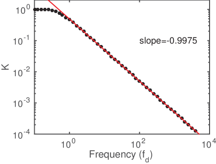
Figure 1: Log-log plot for relationship between the upper bound $K_{F}$ and the frequency $f_{d}=1/d$ when $d$ is a constant.

2.2 Deterministic Brownian motion generated from delay differential equation

Now, we re-examine the delay differential equation (4). Here, the force term $f(t)=\sin(2\pi\beta v(t-1))$ is given by the chaotic solution $v(t)$, which switches between positive and negative. In previous studies, we have seen that the upper bound $K$ changes with $\beta$ according to the power law $K\sim\beta^{-1/2}$ when $\beta\to\infty$. To associate this power law dependence with the frequency of sign changes in the force $f(t)$, we vary the parameter $\beta$ over the range $\beta\in(3,200)$ and solve the equation (4) to obtain corresponding solutions $v(t;\beta)$ (Fig. 2(a)). For each value $\beta$, the corresponding solution randomly changes between positive and negative over time, and hence $\mathrm{sign}(v(t;\beta))$ randomly switches between $+1$ and $-1$ (Fig. 2(b)). We further find out the average frequency of changing the sign of $v(t)$, which is dependent on $\beta$ in a way $f_{d}\sim\beta^{1/2}$ (Fig. 2(c)). Hence, we would have the power law dependence $K\sim f_{d}^{-1}$, which is verified by numerical simulations shown in Fig. 2(d).

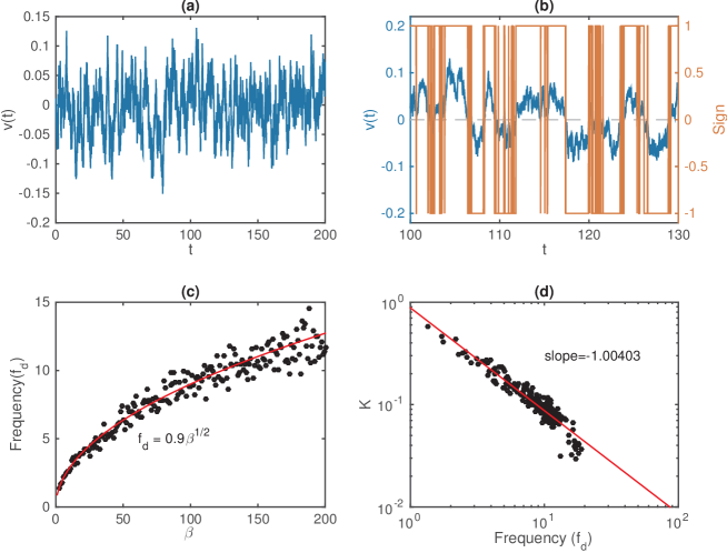
Figure 2: Power law dependence of the delay differential equation model. (a) Solution of the equation (4) with $\beta=52$. (b) Segment of the solution $v(t)$ in (a) and the corresponding sign switches. (c) Relation between the frequency $f_{d}$ of sign changes and the parameter $\beta$, red line shows the fitting of $f_{d}=0.9\beta^{1/2}$. (d) Log-log plot for relationship between the upper bound $K$ and the frequency.

2.3 Random sequences $\{d_{k}\}$

Now, we consider the situations with random sequences $\{d_{k}\}$ with different distributions. From the iterative formula (12), $|v(t_{k})|$ approaches $1$ when $d_{k}$ is large. Hence, it is trivial when $d_{k}$ can always take large values. We are more interested at the situations when $d_{k}$ is mostly small. To this end, we select a family of distributions so that the average $\langle d\rangle$ may approach zero.

Table 1: Distributions of $\{d_{k}\}$

Distribution	Density function	Mean	Variance	CV
exponential distribution	$\lambda e^{-\lambda x}$	$\frac{1}{\lambda}$	$\frac{1}{\lambda^{2}}$	$1$
gamma distribution	$\frac{\beta^{\alpha}}{\Gamma(\alpha)}x^{\alpha-1}e^{-\beta x}$	$\frac{\alpha}{\beta}$	$\frac{\alpha}{\beta^{2}}$	$1/\sqrt{\alpha}$
beta distribution	$\frac{\Gamma(\alpha+\beta)}{\Gamma(\alpha)\Gamma(\beta)}x^{\alpha-1}(1-x)^{\beta-1}$	$\frac{\alpha}{\alpha+\beta}$	$\frac{\alpha\beta}{(\alpha+\beta)^{2}(\alpha+\beta+1)}$	$\sqrt{\frac{\beta}{\alpha(\alpha+\beta+1)}}$
lognormal distribution	$\frac{1}{\sqrt{2\pi}x\sigma}e^{-(\ln x-\mu)^{2}/(2\sigma^{2}))}$	$e^{\mu+\sigma^{2}/2}$	$e^{\sigma^{2}-1}e^{2\mu+\sigma^{2}}$	$\sqrt{e^{\sigma^{2}-1}}$

Here, we consider four type distributions, which are shown in Table  1. According to the mean of these distributions, we can adjust the parameters to ensure that the average interval $\langle d\rangle$ approaches zero with various parameters. For each distribution, we generate random sequences $\{d_{k}\}$ with given parameters, and find the upper bound $K_{F}$ according to (12) and (13). Fig. 3 shows the log-log plots of the upper bound $K_{F}$ versus the frequency $f_{d}$ of the sequences $\{d_{k}\}$. It is obvious to see power law dependences for different distributions of the random sequences.

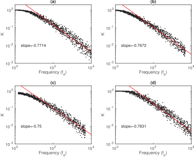
Figure 3: Power law dependence between the upper bound $K_{F}$ and the frequency $f_{d}$. Results show the power law dependences with various distributions for the random sequences $\{d_{k}\}$: (a) exponential distribution with $1<\lambda<1000$, (b) gamma distribution with $\alpha=2$ and $1<\beta<1000$; (c) beta distribution with $\alpha=2$ and $1<\beta<1000$; (d) lognormal distribution with $\sigma=1$ and $-10<\mu<-0.5$.

We note that the slopes in Fig. 3 are different from $-1$ as we have seen in the above discussions of constant $d_{k}\equiv d$. This indicates that the slope may dependences on the some other properties of the distribution. To check this dependence, we consider gamma distribution, beta distribution, and lognormal distribution sequences with varying the coefficient of variation (CV). The coefficient of variation is often used to describe the fluctuation of a random process, and is defined as the ratio of the standard deviation to the mean, which are given in Table 1. Results are shown in Fig. 4, in which power law dependence can be applied to fit the relationship between the upper bound $K_{F}$ and the frequency $f_{d}$ for random sequences $\{d_{k}\}$ with different values CV. We note that the slopes may depends on CV, which show increase with CV for the three type distributions. Particularly, the slope approaches $-1$ when CV decreases to $0$, which is consistent with the above result of constant sequences $d_{k}\equiv d$.

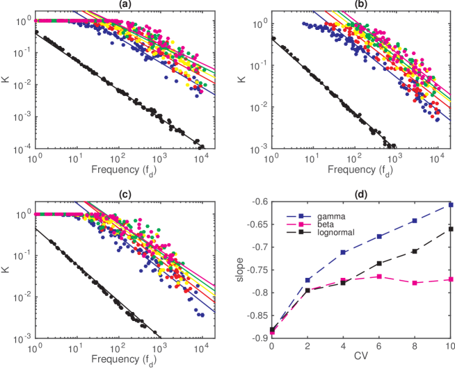
Figure 4: Power law dependences with different CV values. (a) Log-log plot for the relationship between the upper bound $K_{F}$ and the frequency for gamma distribution $\{d_{k}\}$ with various CV. (b) Log-log plot for the relationship between upper bound $K_{F}$ and the frequency for beta distribution $\{d_{k}\}$ with various CV. (c) Log-log plot for the relationship between upper bound $K_{F}$ and the frequency for lognormal distribution $\{d_{k}\}$ with various CV. (d) Dependence of the slopes in (a)-(c) and CV. In (a)-(c), lines show the fitting with power law dependence, results obtained from different values CV ($\mathrm{CV}=0.01,2,4,6,8,10$) are represented by different color.

3 Frequency modulation and amplitude modulation

Previous discussions shown that the upper bound of the equation

$$\dfrac{dv}{dt}=-\gamma v+F(t)$$ (16)

can be modulated by the frequency of switching the sign of perturbation $F(t)$, in a way of power law dependence. Thus, the equation of form (16) can be served as a transformation from frequency modulation to amplitude modulation. Particularly, for a dynamic system with bistable steady states separated by an energy barrier, we may control the frequency of steady state switches by regulating of the frequency in the perturbation function.

To examine this idea, we consider the equation of form

$$\dfrac{dx}{dt}=-\phi^{\prime}(x)+F(t),\quad\phi(x)=x^{2}-2x^{3}+x^{4},$$ (17)

where the perturbation function $F(t)$ is defined as (8), with sequence $\{d_{k}\}$ taken from lognormal distribution with parameters $\sigma=1$ and $-6.0<\mu<-0.5$. The potential function $\phi(x)$ has a form of double well, so that the equation (17) has two steady states $x_{1}^{*}=0$ and $x_{2}^{*}=1$, which are separated by an energy barrier at $x=0.5$ (Fig. 5a).

When there is a perturbation, while we linearize the equation (17) at a steady state $x=x^{*}$, we obtained

$$\dfrac{dx}{dt}=-\gamma(x-x^{*})+F(t)+o(|x-x^{*}|).$$ (18)

Previous discussions shown that the upper bound $|x(t)-x^{*}|$ of (18) is determined by the frequency $f_{d}$ according to a power law dependence. Moreover, when the upper bound $|x(t)-x^{*}|$ is larger than the barrier $x=0.5$, the state can switch from one state to the other one. Hence, we would expect to regulate the frequency of the switching behavior between two steady states $x_{1}^{*}$ and $x_{2}^{*}$ by modulating the parameter $\mu$ in defining the random sequence $\{d_{k}\}$.

From Table  1, the mean value of $\{d_{k}\}$ is given by the parameter $\mu$ as $\langle d_{k}\rangle=e^{\mu+1/2}$, hence, the frequency $f_{d}=1/\langle d_{k}\rangle=e^{-(\mu+1/2)}$. We vary the parameter $-6<\mu<-0.5$, so that the frequency $f_{d}$ changes over the range $1<f_{d}<e^{5.5}$. For each $\mu$, we generate a random sequence $\{d_{k}\}$ and solve the equation (17) with initial condition $x(0)=0$. For each solution, we calculate the average survival time (AST) of the state $x_{1}^{*}=0$, which are shown in Fig. 5b (here $\mathrm{AST}=120$ means no switches from $x_{1}^{*}$ to $x_{2}^{*}$). From Fig. 5b, there is a threshold $\mu^{*}$, so that when $\mu<\mu^{*}$, switches from $x_{1}^{*}$ to $x_{2}^{*}$ do not occur during simulation, i.e., the state $x_{1}^{*}$ is stable under random perturbation. When $\mu>\mu^{*}$, the solution $x(t)$ can leave the state $x_{1}^{*}$, and the AST of $x_{1}^{*}$ decreases with the increasing of $\mu$ (decreasing of the frequency $f_{d}$). Specifically, two sample solutions, with $\mu$ marked with red diamond and blue pentagram in (b), are shown in Fig. 5c-d, respectively. Moreover, density of the solution trajectories $x(t)$ with different $\mu$ values are given in Fig. 5e, which show the changes of the density function with random sequences $\{d_{k}\}$ in defining the perturbation function $F(t)$. These results suggest that the frequency of steady state switches can be regulated by modulating the parameter $\mu$ in defining the random sequence $\{d_{k}\}$.

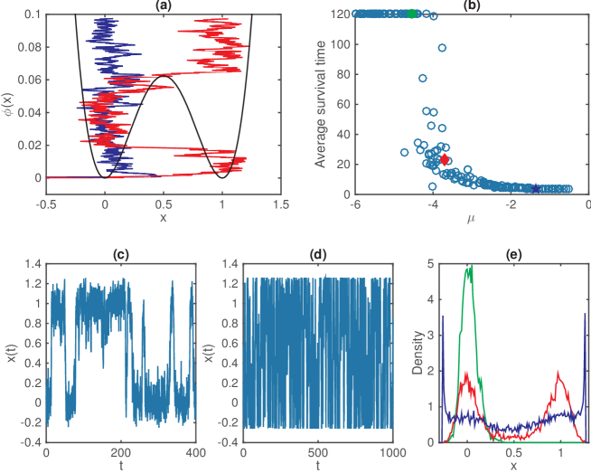
Figure 5: Steady state switches induced by random perturbation. (a) Potential function. Blue and red lines show superposition of two sample solutions that either stay at one local minimal or switches between two local minimal states, respectively. Here, $\mu=-4.538$ for the blue line, and $\mu=-3.7401$ for the red line. (b) Dependence of the average survival time of state $x^{*}=0$ versus the parameter $\mu$ of the random sequence $\{d_{k}\}$. (c) Sample solution with $\mu$ taken from the red diamond in (b). (d) Sample solution with $\mu$ taken from the blue pentagram in (b). (e) Density functions of the solution trajectories $x(t)$ with different $\mu$ values from (b), green square, red diamond, and blue pentagram, respectively.

4 Conclusion

This paper studies the random equation of form (6), which is often applied to model a decay system with randomly switches forces. We explore how the maximum displacement from the equilibrium state depends on the statistical properties of the time points of random force switches. We show that the frequency of random forces switches is essential for the maximum displacement, and there is a power law dependences between the upper bound and the frequency. The slope of the power law dependence is dependent on different distributions of the random sequence $\{d_{k}\}$ which is the base to define the random perturbation. Thus, the random equation of form (6) can be served as a transformation from frequency modulation to amplitude modulation, and regulation of the perturbation frequency can be applied to modulated the stability and state transition in systems with multiple steady states.

Moreover, we re-examine the determined Brownian motion (4) defined by nonlinear delay differential equations. We show that the frequency of sign changes of the ‘chaotic’ solution depends on the equation parameter $\beta$ in an order of $\beta^{1/2}$, and the upper bound of the solution depends on the frequency with a power law $K\sim f_{d}^{-1}$, and hence we confirm the dependence $K\sim\beta^{-1/2}$ reported in previous studies[1].

References

- [1] J. Lei, M. Mackey, Deterministic Brownian motion generated from differential delay equations, Phys Rev E 84 (4) (2011) 041105.
- [2] C. Beck, Higher correlation functions of chaotic dynamical systems-a graph theoretical approach, Nonlinearity 4 (1991) 1131.
- [3] L. Y. Chew, C. Ting, Microscopic chaos and Gaussian diffusion processes, Physica A 307 (2002) 275–296.
- [4] M. Mackey, M. Tyran-Kaminska, Deterministic Brownian motion: The effects of perturbing a dynamical system by a chaotic semi-dynamical system, Phys Rep 422 (5) (2006) 167–222.
- [5] U. an der Heiden, M. C. Mackey, The dynamics of production and destruction: Analytic insight into complex behavior, J Math Biol 16 (1) (1982) 75–101. doi:10.1007/bf00275162.
- [6] B. Dorizzi, B. Grammaticos, M. L. Berre, Y. Pomeau, E. Ressayre, A. Tallet, Statistics and dimension of chaos in differential delay systems, Phys Rev A 35 (1) (1987) 328–339. doi:10.1103/physreva.35.328.