Safe Policy Learning under Regression Discontinuity Designs with Multiple Cutoffs††thanks: Imai acknowledges partial support from the Sloan Foundation (Economics Program; 2020-13946). We thank Tatiana Velasco and her co-authors for sharing the dataset analyzed in this paper. We have benefited from the Alexander and Diviya Magaro Peer Pre-Review Program.
Abstract
The regression discontinuity (RD) design is widely used for program evaluation with observational data. The primary focus of the existing literature has been the estimation of the local average treatment effect at the existing treatment cutoff. In contrast, we consider policy learning under the RD design. Because the treatment assignment mechanism is deterministic, learning better treatment cutoffs requires extrapolation. We develop a robust optimization approach to finding optimal treatment cutoffs that improve upon the existing ones. We first decompose the expected utility into point-identifiable and unidentifiable components. We then propose an efficient doubly-robust estimator for the identifiable parts. To account for the unidentifiable components, we leverage the existence of multiple cutoffs that are common under the RD design. Specifically, we assume that the heterogeneity in the conditional expectations of potential outcomes across different groups vary smoothly along the running variable. Under this assumption, we minimize the worst case utility loss relative to the status quo policy. The resulting new treatment cutoffs have a safety guarantee that they will not yield a worse overall outcome than the existing cutoffs. Finally, we establish the asymptotic regret bounds for the learned policy using semi-parametric efficiency theory. We apply the proposed methodology to empirical and simulated data sets.
Keywords: extrapolation, doubly robust estimation, partial identification, robust optimization
.tocmtchapter \etocsettagdepthmtchaptersubsection \etocsettagdepthmtappendixnone
1 Introduction
The regression discontinuity (RD) design is widely used in causal inference and program evaluation with observational data (e.g., Thistlethwaite and Campbell, 1960; Lee et al., 2004; Eggers and Hainmueller, 2009; Card et al., 2009; Lee and Lemieux, 2010). A primary reason for this popularity is that the RD design can provide credible causal inference without assuming that the treatment is unconfounded. Under the RD design, one can exploit a known deterministic treatment assignment mechanism and identify the average treatment effect at the treatment assignment cutoff. On the whole, the causal inference literature has focused on the development of rigorous estimation and inference methodology for this RD treatment effect (Calonico et al., 2014, 2018; Cheng et al., 1997; Armstrong and Kolesár, 2018; Hahn et al., 2001; Imbens and Lemieux, 2008; Kolesár and Rothe, 2018; Imbens and Wager, 2019).
While treatment effect estimation at the existing cutoff is useful, policy makers may be interested in improving the outcome by considering alternative treatment assignment cutoffs (Heckman and Vytlacil, 2005). Despite the widespread use of the RD design, there has been limited research on policy learning under this design. We address this gap in the literature by developing a methodology for learning new and better cutoffs from observed data. Because the treatment assignment mechanism is deterministic under the RD design, learning a new policy requires extrapolation. Building on the robust optimization framework proposed by Ben-Michael et al. (2021), we develop a safe policy learning methodology under the RD design. Specifically, we provide a theoretical safety guarantee that a new, learned policy will not yield a worse overall utility than the existing status quo policy.
In many applications of the RD designs, the treatment assignment cutoff varies across subpopulations based on certain criteria including geographical regions, time periods, and age groups (e.g., Chay et al., 2005; Klašnja and Titiunik, 2017). We show how to exploit the existence of such multiple cutoffs to make the required extrapolation more credible. Specifically, we compare the conditional potential outcome functions across different sub-populations and assume that the cross-group difference is a smooth function of the running variable with a bounded slope in the extrapolation region. Based on this smoothness assumption, we separate the expected utility into point-identified and partially-identified components, and propose a doubly-robust estimator for the point-identifiable component. We then minimize the worst case utility loss relative to the status quo policy. The resulting policy, based on new treatment cutoffs, has a safety guarantee that they will not yield a worse overall utility than the existing cutoffs. We also establish the asymptotic regret bounds for the learned safe policy using semiparametric efficiency theory.
We apply the proposed methodology to a recent study of the ACCES loan program in Colombia (Melguizo et al., 2016). In this application, geographical departments in Colombia used different cutoffs, which are based on test scores, to determine the eligibility for financial aid to low-income students. We use the proposed methodology to learn a better cutoff for each department to improve the overall enrollment in post-secondary institution throughout the country.
Related Work.
There exist few prior studies that consider policy learning under the RD design. As noted above, many existing studies focus on the identification, estimation, and inference of the average treatment effects at cutoffs. Recently, some scholars have developed extrapolation methods to improve the external validity of the RD design (e.g., Mealli and Rampichini, 2012; Dong and Lewbel, 2015; Angrist and Rokkanen, 2015; Cattaneo et al., 2020; Dowd, 2021; Bertanha and Imbens, 2020). For example, Dong and Lewbel (2015) consider how an infinitesimal change of the cutoff alters the RD treatment effect by estimating its derivative at the existing cutoff. Eckles et al. (2020) propose a different randomization-based framework that exploits measurement error in the running variable and examine how a change in the cutoff value affects the observed outcome. Although the methods proposed in these studies are related to ours, none explicitly considers the problem of policy learning under the RD design.
Our proposed methodology leverages the existence of multiple cutoffs. In most applied studies with multi-cutoff RD designs, however, researchers simply pool sub-populations and normalize the running variable such that the standard single-cutoff RD methodology can be applied. An important exception is Cattaneo et al. (2020), who propose a methodology to extrapolate treatment effects under the RD design with two cutoffs. The authors rely on a parallel-trend assumption that the difference in the conditional expectation of potential outcome between the two groups is constant in the running variable. We generalize and weaken their assumption by allowing the the cross-group difference to change smoothly in the running variable. In addition, while Cattaneo et al. (2020) focuses on the treatment effect estimation with two cutoffs, we propose a policy learning methodology under the general multi-cutoff RD designs.
We also contribute to a growing literature on policy learning with observational data. We found no prior work in this literature that studies the RD design. In addition, most previous work relies upon inverse probability weighting (IPW) (e.g, Qian and Murphy, 2011; Zhao et al., 2012; Kitagawa and Tetenov, 2018a) or doubly-robust augmented IPW (AIPW) (e.g, Athey and Wager, 2021) to estimate and optimize the overall expected utility. In contrast, we adopt the robust optimization framework recently proposed by Ben-Michael et al. (2021) and develop a safe policy learning methodology under the RD design. Related to our approach, some researchers also have used partial identification for policy evaluation (Khan et al., 2023) or to learn an optimal policy in different non-standard settings (e.g., Cui and Tchetgen Tchetgen, 2021; Han, 2019), while others have applied robust optimization (e.g., Kallus and Zhou, 2018; Pu and Zhang, 2021; Gupta et al., 2020; Bertsimas et al., 2023).
Organization of the paper.
The paper is organized as follows. Section 2 defines the policy learning problem in RD designs with multiple cutoffs. Section 3 presents the proposed methodological framework and our smoothness assumption for partial identification. Section 4 discusses the empirical policy learning problem, where we propose a doubly-robust estimator. Section 5 establishes asymptotic bounds on the utility loss of our learned policy relative to the baseline policy and the oracle optimal-in-class policy. In Section 6, we apply the proposed methodology to learning new cutoffs for the ACCES loan program in Colombia. Lastly, Section 7 concludes.
2 Problem setup and notation
We begin by describing the policy learning problem under the general multi-cutoff RD design and introducing formal notation used throughout the paper.
2.1 The multi-cutoff RD design
In our setting, for each unit , we observe a univariate running variable , a binary treatment assignment , and an outcome variable . We assume that the running variable has a continuous positive density on the support . Each unit belongs to one of different subgroups, denoted by , where each group has a corresponding cutoff value . These existing cutoff values may differ between groups. For simplicity, we assume there are no ties, but note that our proposed methodology can still be applied in situations where tied cutoffs may exist. We also assume that these cutoffs have been sorted in an increasing order (i.e., ). Note that both and are pre-treatment variables, which are neither affected by the cutoffs nor the treatment variable.
Throughout the paper, we consider the sharp RD setting, where given a set of known cutoff values , the treatment assignment is completely determined by both the running variable and the group indicator . Specifically, unit in group is assigned to the treatment condition when the value of the running variable exceeds a fixed, known treatment cutoff , i.e.,
where denoting the indicator function. Following the potential outcome framework (Neyman, 1923; Rubin, 1974), we define and as the potential outcomes under the treatment and control conditions, respectively. The observed outcome then is given by . We further assume that the tuples are drawn i.i.d from an overall target population . For notational convenience, we will sometimes drop the unit subscript from random variables.
Much of the RD design literature has focused on the evaluation of the conditional average treatment effect (CATE) at the cutoff. Under the multi-cutoff RD design, we define the group-specific CATE for each group at the cutoff value ,
The key identification assumption for under the sharp RD design is the continuity of the conditional expectation function of the potential outcome (Hahn et al., 2001).
Assumption 1 (Continuity).
Let denote the group-specific conditional potential outcome function. Assume that is continuous in for and .
Under this assumption, we can identify via,
Under Assumption 1 alone, however, the deterministic treatment assignment makes it impossible to identify the average treatment effect beyond the existing cutoff (e.g., Hahn et al., 2001; Imbens and Lemieux, 2008). In the literature, researchers have proposed additional assumptions to extrapolate beyond the existing cutoffs. For example, under the single-cutoff RD setting, Dowd (2021) assume the bounded partial derivative of the conditional expectation function with respect to the running variable. Under the fuzzy RD setting, Bertanha (2020) restricts heterogeneity across compliance classes. Lastly, under the multi-cutoff RD design, Cattaneo et al. (2020) propose a “common-trend” assumption. Building on these recent advancements, we show how to learn new and improved cutoffs from observed data under multi-cutoff RD design.
2.2 Policy learning under the multi-cutoff RD design
We introduce our policy learning problem under the multi-cutoff RD design. Throughout, we assume that potential outcomes depend on cutoffs only through the treatment assignment, which is implicit in our notation (Dong and Lewbel, 2015; Bertanha, 2020). In other words, changing the cutoff value does not alter outcomes unless it leads to a change in the treatment condition. The assumption is violated, for example, if individuals change their behavior in response to a change in the cutoff value under the same treatment condition.
Under the multi-cutoff RD design, a policy is a deterministic function that maps the running variable and group indicator to a binary treatment assignment variable, . Let denote the utility for outcome under treatment . Thus, the utility for unit with treatment and potential outcome is given by . Our goal is to find a new policy that has a high average value (expected utility) for the overall population. For the ease of exposition, we use the observed outcome as the utility, i.e., , but our discussion below readily extends to other utility functions. In Section 6, we consider an adjusted utility function that takes into account the cost of treatment.
For any given policy , we define its overall value as the expected outcome in the target population :
| (1) |
where the expectation is taken with respect to the joint distribution of the running variable , the group indicator , and potential outcomes . The goal of policy learning is to find the best possible policy within a pre-specified policy class , i.e.,
Under the multi-cutoff RD design, we first consider the following class of (group-specific) linear threshold policies:
| (2) |
where each group-specific cutoff value corresponds to a candidate policy for group . We note that the baseline cutoff value may be different from , but both belong to this policy class. Furthermore, we assume that the candidate group-specific policies (cutoffs) in are independent of one another.
Learning an optimal policy requires the evaluation of for any given policy . Under RD designs, however, the average potential outcomes under cutoffs that are different from the existing ones are not identifiable. Since the treatment assignment is deterministic rather than stochastic, the usual overlap assumption, i.e., , is violated under the RD designs. As a result, we cannot use standard policy learning methodology based on the inverse probability-of-treatment weighting (IPW) or its variants (see, e.g. Zhao et al., 2012; Kitagawa and Tetenov, 2018b; Athey and Wager, 2021). Therefore, to evaluate , we must extrapolate beyond the existing threshold and infer the average unobserved potential outcomes.
3 Safe policy learning through robust optimization
We now outline our basic framework of policy learning under the multi-cutoff RD designs. The proposed framework has three steps. We first decompose the expected utility for any given policy into identifiable and unidentifiable components. Second, we partially identify the unidentifiable component using a relaxed version of the “parallel-trends” assumption from the difference-in-differences literature (Rambachan and Roth, 2023). Lastly, we propose a robust optimization approach that minimizes the worst case utility loss relative to the baseline policy. We show that the resulting minimax optimal policy has a safety guarantee; the utility of deploying the learned policy is no worse than the baseline policy under the assumption used for partial identification.
3.1 Policy value decomposition
We begin by defining the baseline policy that generates the observed data as
Note that this baseline policy is contained in the linear-threshold policy class defined in Equation (2). By comparing the deviation of a given policy from the baseline policy , we decompose the expected utility in Equation (1) into point-identifiable and non-identifiable terms, denoted by and , respectively:
| (3) | ||||
where is the group-specific conditional potential outcome function.
The first term in Equation (3) corresponds to the cases where the policy agrees with the baseline policy . This component can be point-identified from the observable data by replacing the counterfactual outcome with the observed outcome . The second and third terms, however, are not point-identifiable without further assumptions; the counterfactual outcome cannot be observed when the policy under consideration disagrees with the baseline policy .
We consider the following restricted set of group-specific linear threshold policies,
| (4) |
Like the unrestricted policy class in Equation (2), this policy class contains the baseline policy . In this policy class, however, the new cutoffs are found between the lowest and highest cutoffs, denoted by and , respectively. The reason for this restriction is that the observed data provide no information to leverage beyond this range. For example, above the highest cutoff , all units receive the treatment and no outcome is observed under the control condition.
Under this restricted policy class , the unidentifiable term can be further decomposed into the conditional mean function of the observed outcome, which is point-identifiable, and an unidentifiable “difference function,”
| (5) | ||||
| (6) |
The difference function represents the difference in the conditional mean function of potential outcomes between two groups at the same value of the running variable.
Note that if , then the conditional average treatment effect is identical between groups and given the running variable. This type of assumption is often invoked to combine treatment effect estimates from multiple studies (Stuart et al., 2011; Dahabreh et al., 2019), but it is typically not credible here because the running variable is the only conditioning variable. In Section 3.2, we will instead partially identify the difference function by requiring a weaker assumption that the difference function is a smooth function of the running variable.
We now formally state our decomposition result, showing that we can use the group whose existing cutoff is closest to the counterfactual cutoff of another group for extrapolation.
Proposition 1 (Decomposition of the unidentifiable component).
For any policy , the unidentifiable term in Equation (3) can be further decomposed as follows:
where is identifiable but is not,
| (7) | ||||
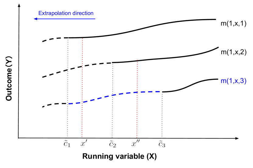
Figure 1 illustrates the decomposition using a three-group case and focusing on the outcome under the treatment. Suppose that we wish to learn a new cutoff for Group 3 whose existing cutoff is . To do this, we must extrapolate the conditional mean outcome for this group in the region below the existing cutoff (represented by the dashed blue line). To evaluate the counterfactual value of the conditional mean outcome at for Group 3, we choose Group 2 whose existing cutoff is the closest to . We then decompose the counterfactual value into the identifiable conditional mean for Group 2, i.e., , and the difference in the conditional mean function between Groups 3 and 2, i.e., . Similarly, to infer , we use Group 1 as a reference group and decompose this counterfactual value into the identifiable conditional mean value for Group 1, i.e., , and the difference between Groups 3 and 1, i.e., .
There are other constructions of decomposing , depending on the chosen reference group for comparison. We discuss an alternative decomposition in Appendix A.1. Although we focus on the decomposition in Proposition 1 in this paper, it is straightforward to adapt our methodology below to other decompositions.
In sum, Proposition 1 implies the following decomposition of the expected utility in Equation (3):
| (8) |
For any given policy , when the baseline policy and a candidate policy agree, the expected utility equals the identifiable component . When they disagree, the expected utility equals the sum of two components: the identifiable term , and the partially identifiable term .
3.2 Partial identification and robust optimization approach
Using the decomposition above, we propose a robust optimization approach to policy learning. Specifically, we first partially identify the difference function and then use robust optimization to derive an optimal policy by maximizing the worst case value.
As illustrated in Figure 1 and discussed above, the cross-group difference in the conditional outcome needed for extrapolation is not identifiable. For example, at , this difference function between Groups 3 and 2 cannot be point-identified. Yet, the same difference function is identifiable in the region above the existing cutoff of Group 3, i.e., . We leverage this fact for extrapolation under the following assumption that the cross-group difference changes smoothly as a function of the running variable.
Assumption 2 (Smooth Difference Function).
The difference function lies in the following function class,
where is a group index, and is a positive constant for and .
In the function class , the group index depends on the treatment condition. For example, in the case of the conditional outcome model under the treatment, represents one of the two groups — Groups and — with a higher cutoff, whereas under the control condition it corresponds to the group with a lower cutoff. Thus, equals the boundary point at which the difference model can be identified.
Assumption 2 states that the cross-group heterogeneity is a smooth function of the running variable with a varying slope, which is assumed to be bounded when the difference function is unidentifiable. The assumption limits the strength of the interaction between the running variable and group indicator in the conditional expected potential outcome. Assumption 2 generalizes and hence weakens the assumption of Cattaneo et al. (2020) who consider an important special case with two groups. Specifically, they assume that the cross-group heterogeneity does not depend on the running variable at all, i.e., implying is constant in . Their assumption is analogous to the parallel trend assumption under the difference-in-differences design.
Note that for some values of the running variable, the difference function is identifiable as . Therefore, under Assumptions 2, we can directly compute the set of potential models for the difference function by extrapolating from the closest boundary point . This leads to the following restricted model class for the difference function,
| (9) |
with the point-wise upper and lower bounds given by
| (10) | ||||
where represents a set of values of the running variable, for which the baseline policy gives the treatment condition to group . Note that the limits are taken as the value of the running variable approaches the baseline cutoff from within .
Finally, we use robust optimization to find an optimal policy. We do so by maximizing the worst case value of the expected utility in Equation (8) over the restricted policy class , with the difference function taking values in the ambiguity set :
| (11) |
As Ben-Michael et al. (2021) show, the resulting policy has a safety guarantee that the overall expected utility of the learned policy is no less than that of the baseline policy. This safety property holds because maximizes the worst case value when it disagrees with the baseline policy.
4 Empirical policy learning
In the previous section, we define the population optimal policy that maximizes the worst case value of the population expected utility for any given policy . Next, we show how to construct this maximin policy empirically using a finite amount of observed data. Recalling our decomposition in Proposition 1, the inner optimization problem of Equation (11) can be decomposed into the sum of three components, where the first two components, and , are point-identifiable, while the last term is not. We introduce our proposed estimator by examining each of these three terms in turn.
4.1 Doubly robust estimation
Since the first term in Equation (3) is identifiable, we use its sample analog for unbiased estimation:
| (12) |
The second term in Equation (7) is also nonparametrically identified, but this term contains an unknown nuisance component, corresponding to the conditional outcome regression for each group , . We compute the efficient influence function for estimating , which yields the following equivalent representation,
| (13) | ||||
where is the the conditional probability of group membership given the value of the running variable .
Although Equation (13) resembles the standard doubly robust construction, the nuisance model represents the conditional probability of group membership given the running variable rather than the conditional probability of treatment assignment. This difference has a couple of implications. First, the proposed framework does not require the unconfoundedness of group membership. This contrasts with the standard doubly robust estimator which assumes the treatment assignment to be unconfounded. Second, the nuisance model is a function of a single-dimensional running variable, making it substantially easier to estimate robustly than typical propensity score models.
We adopt a fully nonparametric approach to estimating these nuisance components and and use cross-fitting (Chernozhukov et al., 2016; Athey and Wager, 2021). Since the running variable is one dimensional, many potential nonparametric estimators can be used. In our empirical analyses (Section 6), we fit a local linear regression for available in the R-package nprobust and fit a multinomial logisitic regression for based on a single hidden layer neural network of the R package nnet.
For cross-fitting, we randomly split the data into disjoint folds, where each fold contains a subset of data from all groups. For each fold , we use the remaining folds to estimate the nuisance components and then compute the estimates on fold . We denote these estimates by and , where we use the superscript to denote the model fitted to all but the fold that contains the th observation. Now, we can write the proposed cross-fitted doubly-robust estimator as,
| (14) | ||||
This doubly robust estimator achieves semiparametric efficiency while only requiring mild sub-parametric convergence rate conditions of the two nuisance models and (see Assumption 5). In Section 5, we show that this rate-double robustness property allows us to learn an empirical worst-case policy at a fast rate.
4.2 Estimating the bounds
We now turn to estimating the worst-case value of in Equation (7). We first define the sample analog of as follows:
| (15) | ||||
Unfortunately, it is not possible to directly optimize over the restricted model class because a model in this class contains an unknown nuisance component . This term appears in the point-wise upper and lower bounds, and . In Appendix A.2, we propose an efficient two-stage doubly robust estimator that has a fast convergence rate. This model builds upon the DR-learner developed for estimating the conditional average treatment effect (Kennedy, 2020).
We construct an empirical model class by plugging in the estimates in place of their true values given in Equation (10). The empirical bounds, and , for any value of , are given by:
| (16) | ||||
We discuss choosing values of the smoothness parameter in Section 4.3 below.
With these three components in place, we obtain an empirical optimal policy by maximizing the worst-case in-sample value across policies :
| (17) |
4.3 Choosing the smoothness parameter
Smoothness restrictions are often used to obtain partial identification (e.g., Manski, 1997; Kim et al., 2018). Similar to these cases, Assumption 2 requires a priori knowledge of the degree of smoothness, directly controlled by the corresponding smoothness parameter . A greater value of will lead to a more conservative policy whose new thresholds are closer to the original ones. In principle, the choice of the smoothing parameter value should be guided by subject-matter expertise. Here, we propose a default data-driven method based on the assumption that the least smooth area of the difference function occurs in the region of overlapping policies between the two groups (Rambachan and Roth, 2023).
To choose the value of , we leverage our proposed two-stage doubly robust estimation procedure described in Appendix A.2. In short, we first construct a DR pseudo-outcome for the actual observed difference . We then fit a local polynomial regression with the running variable as the only predictor. The fitted nonparametric model also yields the estimates of their first local derivatives based on the local polynomial regression method proposed by Calonico et al. (2018, 2020). We compute the absolute value of the estimated first-order derivative at a grid of points in the region of overlapping policies between the two groups, and take the maximum value as . In practice, as illustrated in Section 6, we recommend considering a range of plausible values of , e.g., multiplying those estimates by a constant, e.g., 2, 4, and 8, and conducting a sensitivity analysis to illustrate the sensitivity of learned policies to the strength of the smoothness assumption (see Rambachan and Roth (2023); Kim et al. (2018); Imbens and Wager (2019) for a similar practical advice).
5 Theoretical guarantees
To better understand the statistical properties of the learned policy described above, we compute an asymptotic bound on the utility loss relative to the baseline policy and the oracle optimal policy within the policy class.
5.1 Assumptions
Throughout, we maintain the following additional assumptions. First, as in the existing policy learning literature (e.g., Zhou et al., 2018; Nie et al., 2021; Zhan et al., 2021), we assume that the potential outcomes are bounded.
Assumption 3 (Bounded outcome).
There exists a such that .
This bounded assumption can be generalized to unbounded but sub-Gaussian random variables (Zhou et al., 2018; Athey and Wager, 2021).
Second, we assume the existence of overlap between groups in terms of the running variable.
Assumption 4 (Overlap between groups based on the running variable).
There exists some such that for all and .
Unlike the standard DR estimators in observational studies, we neither require the covariate overlap nor unconfoundedness for the treatment assignment. Indeed, the proposed methodological framework does not require group membership to be unconfounded either.
Third, we assume that it is possible to estimate the nuisance components of (Equation (13)) well.
Assumption 5.
For every fold :
| (18) |
and for every and , :
| (19) |
where is taken to be an independent test sample drawn according to the density .
The assumption allows us to obtain tight regret bounds for learning policies using the proof strategy of Zhou et al. (2018) (see also Chernozhukov et al., 2016; Athey and Wager, 2021). Under the multi-cutoff RD design, Assumption 5 is reasonable since the running variable is one-dimensional. This is in stark contrast with typical observational studies where one must adjust for many observed confounders.
Finally, we quantify the effect of using the estimated empirical bounds on the regret of the learned policy by invoking the following assumption that characterizes this error rate. Here, we make the necessary assumption on the lower bounds since the inner optimization problem of Equation (17) depends only on the worst value of , i.e, .
Assumption 6 (Empirical Bound Estimation Error).
For some sequence , assume that
The definitions of the lower bounds in Equations (10) and (16) imply,
| (20) | ||||
Thus, the resulting error depends on the accuracy of estimating the conditional cross-group difference function at the existing discrete cutoff values . To keep our results general, we do not specify the exact rate of below but discuss some special cases.
5.2 Performance relative to the baseline policy
Under the above assumptions, we compare the learned policy to the baseline policy as well as the oracle policy that maximizes the expected utility. To simplify the statement of the main theorem, we first define and as the doubly-robust scores for Group used to extrapolate to the left (from the treated to the control) and right (from the control to the treated) of the current cutoff, respectively:
| (21) | ||||
To characterize the safety property of our learned policy , we first bound the utility loss relative to the baseline policy . Here, we report the simplified version of this bound, and provide a more general version in Appendix C.3.
Theorem 1 (Statistical safety guarantee).
The theorem ensures, asymptotically, that the learned policy will not yield a worse overall utility than the baseline policy. The constant term in the bound arises from the proposed doubly robust estimator (see also Zhou et al., 2018; Athey and Wager, 2021). In addition, the rate of convergence depends on the slower of the two estimation error rates: one is the standard , which comes from estimating and , and the other is the estimation error for the empirical model class . This term typically exhibits a slower-than-parametric rate, depending on the accuracy of estimating the local difference at fixed points.
Compared to the optimal regret bound achieved in the standard policy learning settings with perfect point identification (Kallus and Zhou, 2018; Kitagawa and Tetenov, 2018b; Zhan et al., 2021; Athey and Wager, 2021), the presence of this additional error term term is due to the partial identification under multi-cutoff RD designs. Poor estimation of , therefore, could make a learned policy unnecessarily deviate from the baseline policy, leading to the loss of the safety guarantee unless the sample size is sufficiently large.
Remark 1.
Naive estimation of the difference function based on plug-in estimates of two conditional mean outcome functions may inherit large errors due to complexity of the underlying regression functions. Like Kennedy (2020), our proposed estimator in Section 4.2 directly incorporates the smoothness of the heterogeneous difference function . For example, when the nuisance components satisfy certain weak second-order error conditions and is -smooth, the oracle rate for estimating the local at fixed points is given by , because the running variable is uni-dimensional. In contrast to the standard doubly robust estimator of the ATE, this minimax rate is slower than root-, because the parameter is an infinite-dimensional regression curve. As the difference function becomes more smooth, this rate should approach that of the standard ATE case.
Remark 2.
While we derive the asymptotic results as the number of observations increases, the constant term in the regret bound depends on the number of total groups, . In our setup, we assume that these groups are pre-determined, so that the number of groups is fixed. In practice, needs to be much smaller than to make Theorem 1 meaningful.
5.3 Performance relative to the oracle policy
Lastly, we compare our learned policy to the infeasible, oracle optimal policy in the same policy class, defined as:
As before, we report a simpler version of the bound here, while its complete version is found in Appendix C.4.
Theorem 2 (Empirical optimality gap under the multi-cutoff regression discontinuity designs).
Compared to Theorem 1, there is an additional term that is proportional to the smoothness parameter and the average distance to the nearest cutoff. This term measures the sample average of the length of the point-wise partial identification bound for under Assumption 2. While the robust optimization procedure ensures that our learned policy will be no worse than the baseline policy, asymptotically, Theorem 2 shows that this safety guarantee comes at the cost of obtaining a potentially suboptimal policy. If the cross-group difference deviates substantially from a parallel trend, i.e., is larger, then the interval will be wider, leading to a potentially larger optimality gap.
6 Empirical application
In this section, we apply the proposed methodology to the ACCES (Access with Quality to Higher Education) program, which is a national-level subsidized loan program in Colombia. We present additional simulation results evaluating our approach in Appendix B. Starting from 2002, the ACCES program provides financial aid to low-income students. Eligibility for the program is determined by a test score cutoff, which varies across different regions of Colombia and time periods. The original analysis by Melguizo et al. (2016) estimated a single RD treatment effect by pooling and normalizing all 33 cutoffs, while Cattaneo et al. (2020) focused on two cutoffs from different time periods and extrapolated the RD treatment effect for each one. In contrast to these prior studies, we analyze all the cutoffs across different geographical regions at the same time and learn a new safe policy for each one of them by leveraging the existence of multiple cutoffs.
6.1 The background
We begin by providing some background information about the ACCES program (see Melguizo et al. (2016) for more details). To be eligible for the ACCES program, a student must achieve a high score on the national high school exit exam, the SABER 11, administered by the Colombian Institute for the Promotion of Postsecondary Education (ICFES). Each semester of every year, once students take the SABER 11, the ICFES authorities compute a position score that ranges from 1 to 1,000, based on each student’s position in terms of 1,000 quantiles. For example, the students who are assigned a position score of 1 should be in the top 0.1%, while those with the test scores in the bottom 0.1% receive a position score of 1000. The SABER 11 position scores are calculated for each semester, and then pooled for each year. Throughout our analysis, as in Cattaneo et al. (2020), we multiply the position score by so that the values of the running variable above a cutoff lead to the program eligibility.
To select ACCES beneficiaries, the Colombian Institute for Educational Loans and Studies Abroad establishes an eligibility cutoff such that students whose position scores are higher than the cutoff becomes eligible for the ACCES program. The eligibility cutoff is defined separately for each department (or region) of Colombia, and has changed over time. Between 2002 and 2008, the cutoff was for all Colombian departments. After 2008, however, the ICEFES used varying cutoffs across different years and departments.
We analyze the data collected from all 33 departments in 2010, when each department used a different cutoff value. We do not analyze the data from 33 departments whose sample size is less than 200. Given the discrete running variable in this case, the reliable use of local polynomial regression requires a larger sample size (Calonico et al., 2014, 2018). The final dataset includes the observations from 23 different departments of Colombia. Following Melguizo et al. (2016) and Cattaneo et al. (2020), the outcome of interest is an indicator for whether the student enrolls in a postsecondary institution. Table 1 reports the sample size, group-specific baseline cutoff , and estimated group-specific RD treatment effect at the baseline cutoff for each department.
| Department | Sample size | Baseline cutoff | RD Estimate | s.e. |
|---|---|---|---|---|
| Magdalena | 214 | -828 | 0.55 | 0.41 |
| La Guajira | 209 | -824 | 0.57 | 0.31 |
| Bolivar | 646 | -786 | 0 | 0.21 |
| Caqueta | 238 | -779 | 0.56 | 0.35 |
| Cauca | 322 | -774 | 0.02 | 0.78 |
| Cordoba | 500 | -764 | - | 0.26 |
| Cesar | 211 | -758 | 0.53 | 0.37 |
| Sucre | 469 | -755 | 0.11 | |
| Atlantico | 448 | -754 | 0.15 | |
| Arauca | 214 | -753 | -0.7 | 1.11 |
| Valle Del Cauca | 454 | -732 | 0.16 | |
| Antioquia | 416 | -729 | 0.21 | |
| Norte De Santander | 233 | -723 | -0.08 | 0.43 |
| Putumayo | 236 | -719 | -0.47 | 0.79 |
| Tolima | 347 | -716 | 0.12 | 0.31 |
| Huila | 406 | -695 | 0.06 | 0.23 |
| Narino | 463 | -678 | 0.08 | 0.19 |
| Cundinamarca | 403 | -676 | 0.12 | 0.81 |
| Risaralda | 263 | -672 | 0.41 | 0.42 |
| Quindio | 215 | -660 | -0.03 | 0.11 |
| Santander | 437 | -632 | 0.25 | |
| Boyaca | 362 | -618 | 0.48 | 0.36 |
| Distrito Capital | 539 | -559 | 0.14 |
⋆ indicates significant RD treatment effect at the 5% level
6.2 Empirical findings
We estimate the empirical improvement of expected utility, i.e., , for each candidate policy in the policy class , restricting the candidate cutoffs for each department to be within the range of the original lowest and highest cutoffs, i.e., . We select the value of the smoothness parameter for each pairwise difference function under Assumption 2, by applying the procedure described in Section 4.3. We first fit a local polynomial regression of each difference function , and then take the maximal absolute value of the estimated local first derivative at a grid of points as . We also perform a sensitivity analysis by multipling the data-driven choice of by a positive constant and seeing how the learned policy changes.
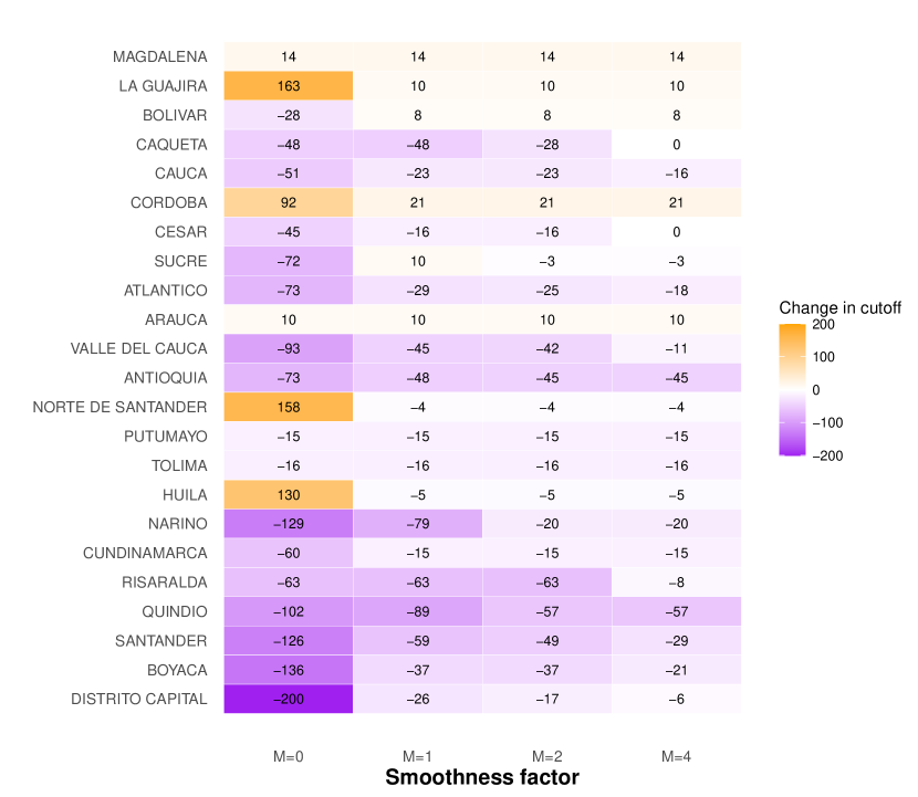
We first consider the stronger parallel-trend assumption that the cutoff differences are exactly constant, i.e., , allowing us to point-identify the counterfactual function . As shown in the first column () in Figure 2, for most departments, the learned cutoffs are lower than the baseline cutoffs (highlighted by purple). Thus, lowering the cutoff, which increases the number of eligible students, is likely to result in a higher overall enrollment rate. This is not surprising, as financial aid typically should help students attend post-secondary institutions.
On the contrary, the learned cutoffs in La Cuarjira, Cordoba, Norte De Santander, and Huila are much greater than the actual baseline cutoffs used. Referring to the summary results in Table 1, however, only Cordoba showed a significant negative treatment effect at the cutoff, while the treatment effect of the other three departments were ambiguous. Therefore, we find that the parallel-trend assumption may be too aggressive and lead to unnecessary policy changes.
Next, we consider a weaker smoothness restriction using the data-driven estimate of , corresponding to the column in Figure 2. These estimated values range from to with a median of for different possible values of and . Overall, we observe that the learned policies are less aggressive compared to the results obtained under the parallel-trend assumption. Although most departments still have reduced cutoffs, the magnitude of the changes is smaller. Notably, the policy changes are now more conservative for those departments that would have seen an increase in the cutoff under the “parallel-trend” assumption. Specifically, Cordoba shows the largest change, aligning with the significant negative treatment effect estimate at the cutoff for Cordoba (see Table 1).
Further, we conduct a sensitivity analysis by varying the multiplicative factor . As shown in Figure 2, the learned policies are relatively robust to the choice of the smoothing parameter, although, as expected, a greater value of results in a more conservative learned policy that is closer to the baseline policy.
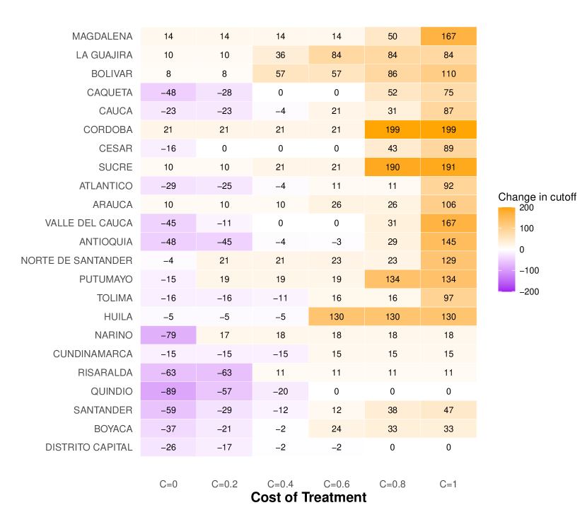
Finally, we incorporate the cost of treatment into the utility function. Given that the outcome enrollment rate is binary, a general utility function for outcome under treatment can be expressed as . Here, represents the utility change in the treatment condition, and can be interpreted as the baseline cost of implementing treatment . Additionally, we assume an equal utility gain of one from enrollment, i.e., . We set the cost of not providing financial aid to zero and the cost of benefiting from the ACCES program to .
Thus, the utility function is of the form . We examine how changing the cost affects the learned policy. We consider a range of values for the cost, , to explore the trade-off between cost and utility. Figure 3 shows the results. Changing the cost of offering a loan yields optimal robust cutoffs that affect the number of eligible students. The overall trend indicates that the learned policy will still lower the cutoffs relative to the baseline for most departments when the cost is low to moderate. Only when the cost is high—when , i.e., we would only offer a loan if the increase in enrollment is larger than 80%—do the cutoffs start to increase, leading to more students being excluded from the program relative to the baseline. Note that in the Distrito Capital, where the baseline cutoff is the highest, the learned cutoff will eventually reach a point where it remains unchanged, due to the restriction that the learned cutoffs cannot exceed the maximum baseline cutoff.
7 Concluding remarks
Despite the popularity of regression discontinuity (RD) designs for program evaluation with observational data, little attention has been given to the question of how to learn new and better treatment assignment cutoffs. In this paper, we proposed a methodology for safe policy learning that guarantees that a new, learned policy performs no worse than the existing status quo. We partially identify the overall utility function and then find an optimal policy in the worst case via robust optimization. We stress, however, that extrapolation is required to learn new policies. Our approach leverages the presence of multiple cutoffs, and is based on a weak, non-parametric smoothness assumption about the level of cross-group heterogeneity.
There are several directions for future research. First, the partial identification assumption we employ involves smoothness parameters. While we have suggested ways that the data can inform these hyperparameters, developing rigorous selection criteria for this choice will be an important aspect of future work.
Second, we can generalize Assumption 2 to the case where it holds only after conditioning on the other available covariates in RD design. Consequently, our proposed doubly robust estimator can be modified to include not only the single running variable, but also other observed covariates.
Third, we can incorporate other constraints such as fairness, risk factors, simplicity, or other functional form constraints into the policy class. For example, candidate treatment cutoffs may be restricted by a lower threshold , i.e., , or federal policymakers want to learn a unified cutoff for all subpopulations, i.e. . In these cases, our robust optimization approach can be directly applied to learn the worst-case optimal policy in the class, although the safety guarantee relative to the status quo may be compromised because the baseline policy may not be included in the policy class.
Fourth, one may consider directly imposing a budget constraint. As shown in our empirical application, we can include a cost into the utility function. This can be viewed as a Lagrangian relaxation of directly imposing a budget constraint. One problem of such direct constraint is that the constraint might not hold in the population. Further investigation of this issue is necessary (Sun, 2021).
Fifth, we can change the target population of interest and expand the notion of safety (Jia et al., 2023). In particular, it is of interest to establish a statistical safety guarantee for a specific group or other well-defined subpopulation so that a learned policy does not perform worse in this subpopulation than the status quo policy. This differs from the current guarantees that hold over the entire population on average, and so can lead to worse outcomes for certain subpopulations.
Finally, one may consider the use of safe policy learning in other study designs. For example, the tie-breaker design of Li and Owen (2022) combines treatment assignment based on both randomization and thresholds. Extending our methodological framework to this and other study designs is left to future work.
Supplementary Appendix for “Safe Policy Learning under Regression Discontinuity Designs with Multiple Cutoffs”
.tocmtappendix \etocsettagdepthmtchapternone \etocsettagdepthmtappendixsubsection
Appendix A Additional details in the main text
A.1 Another way of decomposing
Here we propose another way of decompose the counterfactual outcome for group at , , by looking at all groups with smaller cutoffs than for the treatment condition and all groups with larger cutoffs than for the control condition :
| (A.1) | ||||
Under the special case of only two groups, the above construction coincides with the one given in Equation (7).
A.2 A double robust estimator for heterogeneous cross-group differences
Due to the discontinuity at the cutoffs, we need to estimate the conditional differences between observed treatment groups or between observed control groups using data above or below the threshold, respectively. Below we discuss how to estimate differences across treatment groups using a portion of the data; estimates for the control group can be obtained similarly using the another portion of the data.
Algorithm 1 (Estimating observed conditional differences across treatment groups).
For group and its comparison group , let denote two independent samples of observations of .
Step 1. Nuisance training:
(a) Construct estimates of the group propensity score using .
(b) Construct estimates of the group-specific regression functions using .
Step 2. Pseudo-outcome regression: Construct the pseudo-outcome
and regress it on covariates in the test sample , yielding
for , i.e., the treatment groups.
Here, can represent any generic nonparametric regression methods.
Step 3. Cross-fitting (optional): Repeat Step 1-2, swapping the roles of and so that is used for nuisance training and as the test sample. Use the average of the resulting two estimators as a final estimate of . -fold variants are also possible.
Similarly, to estimate the conditional differences in observed outcome between control groups, we should use another portion of the data and fit the pseudo-outcome regression in Step 2 using .
Appendix B Simulation Studies
In this section, we assess the empirical performance of our safe policy learning approach proposed in the main text through simulation studies. We compare the utility loss of our learned policy relative to the baseline policy and the oracle optimal policy under a special multi-cutoff RD case with only two groups, i.e, the group index .
B.1 The setup
We consider a realistic simulation setting based on the ACCES loan program data analyzed in Section 6. Specifically, the data generating process is given by,
with the sample size . Following Cattaneo et al. (2020) who analyzed a subset of the ACCES data, we focus on two sub-populations with cutoff values and .
Under this setting, the group indicator is determined by the running variable and a Normal random variable , with mean and variance . The value of controls the degree of overlap between the two groups with a higher value leading to a greater overlap. We set so that the conditional probability of belonging to group is roughly between 0.3 and 0.7 for all samples, which gives a strong overlap between the two groups.
The outcome variable is generated according to the following model:
| (B.2) |
where the error term follows a normal distribution with mean 0 and standard deviation of . We consider two data generating scenarios. For both Scenarios, we choose to be a third-order polynomial, and select by first fitting a third-order polynomial model using the data from our empirical application, and then further calibrating the fitted coefficients such that the baseline policy equals the oracle policy under Scenario A, and that the baseline policy differs from the oracle policy under Scenario B. The result are the following two choices:
| (B.3) | ||||
We note that in both scenarios, the true difference in conditional potential outcome functions between the two groups is Lipschitz continuous on , and it is even smoother than the approximately constant cutoff assumption (Assumption 2).
The policy class of interest is parameterized as
Our method learns an optimal policy over the class under Assumption 2 based on Equation (17). We estimate all the nuisance components in Equation (14) via nonparametric methods using the cross-fitting strategy. Specifically, we use a local polynomial regression as implemented in the R package nprobust for and a generalized linear model with logistic link function and a smoothing spline for . To construct the empirical point-wise upper and lower bounds, and , we use our proposed two-stage doubly robust estimator in Appendix A.2 to estimate the unknown nuisance component . Finally, we choose the smoothness parameter through the procedure discussed in Section 4.3.
B.2 Results
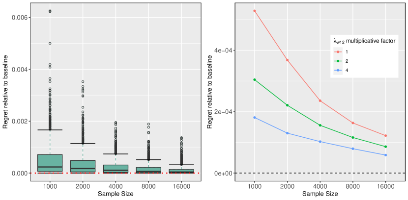
Under Scenarios A and B, we vary both the sample size and the choice of the value of the smoothness parameter , and compare our learned policy with the baseline policy as well as the oracle optimal policy. To vary , we begin with the data-driven approach described in Section 4.3, and then multiply it by larger factors. We first present the results for Scenario A where the baseline policy is optimal in policy class . Figure B.1 shows the utility loss (or regret) of our learned policy relative to the baseline, for different values of sample size (both left and right panels) and smoothness parameter (right panel). The regret is always positive because the baseline policy is optimal. Overall, we find that the regret of the learned policies improves with the sample size , and decreases and approaches zero as gets large. In addition, as shown in right panel of Figure B.1, a larger value of the smoothness parameter leads to more conservative inference, i.e. the learned policy is closer to the baseline, and therefore, in this case, the regret is closer to zero.
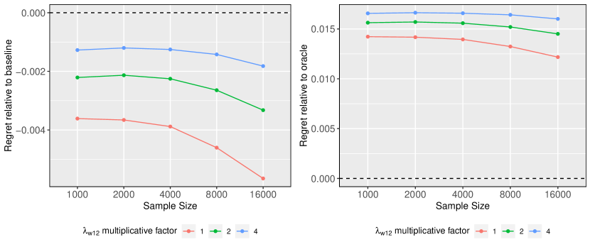
Next, we present the results under Scenario B. Since the baseline policy is no longer optimal, we compute the utility loss/regret of our learned polices relative to the baseline and optimal polices separately. Figure B.2 shows that on average, our empirical safe policy improves over the baseline policy, regardless of the value of smoothness parameter and sample size. This improvement is greater for a smaller value of smoothness parameter, due to the more informative and tighter extrapolation. Furthermore, when comparing to the oracle policy, a smaller value of smoothness parameter yields a greater improvement in regret, which becomes greater as the sample size increases. The regret, however, does not decrease to zero even when the sample size is large. This is because the safe policy can still be sub-optimal due to the lack of point-identification. As we argued in Theorem 2, we find that this suboptimality gap becomes greater as the chosen value of becomes larger.
Appendix C Proofs and Derivations
To help guide the proof in the main paper, we first introduce some useful definitions and lemmas used throughout this section. Recall that under the multi-cutoff RD design, the restricted policy class we consider is defined as . To simplify the notation, we drop the subscript of and use , whenever there is no ambiguity.
C.1 Definitions and lemmas for terms and term
Definition 1 (Rademacher complexity).
Let be a family of functions mapping . The population Rademacher complexity of is defined as
where ’s are i.i.d. Rademacher random variables, i.e., , and the expectation is taken over both the Rademacher variables and the i.i.d. covariates .
Definition 2.
Define the following population quantity,
We also define the following empirical quantity,
supposing the true counterfactual difference function were known.
Lemma C.1.
Under Assumption 3, and considering the policy class , which has finite VC dimension , then for any , we have,
with probability at least , where is a universal constant.
Proof of Lemma C.1.
Define the function class with functions in
Notice that
The class is uniformly bounded by because the outcomes and the difference functions are bounded, so by Theorem in Wainwright (2019)
with probability at least . Finally, the Rademacher complexity for is bounded by
where the constant term in the second inequality is due to and , and the last inequality follows from the fact that for a function class with finite VC dimension , the Rademacher complexity is bounded by, , for some universal constant (Wainwright, 2019, ). Now, the specific policy class has a VC dimension , so let , we obtain the result. ∎
Lemma C.2 (Bounded estimation error).
Under Assumption 6, for any ,
C.2 Definitions and lemmas for term
We now turn our attention to the doubly-robust construction in Equation (13). Our derivation is based upon the proof strategy in Zhou et al. (2018). Again, for simplicity, we drop the subscript of and use throughout this section.
Definition 3.
Corresponding to Equation (13), we redefine the term as the following population quantity, explicitly under a given policy ,
where and is defined as the true double-robust score for group when we extrapolate the current cutoff to the left and to the right, respectively.
To simply the notation, we further define
We also redefine the empirical quantity in Equation (14),
where and are the empirical double robust scores using the cross-fitted nuisance estimates constructed from the folds of the data:
Finally, we define the oracle (infeasible) estimator with the estimated and in substituted by the true value and ,
It can be easily shown that .
To proceed with the proof, we adopt several useful definitions from Zhou et al. (2018).
Definition 4.
Given the feature domain , a policy class , a set of points , define:
-
1.
Hamming distance between any two policies and in .
-
2.
-Hamming covering number of the set : is the smallest number of policies in , such that
-
3.
-Hamming covering number of
-
4.
Entropy integral: .
Definition 5.
The influence difference function and the policy value difference function are defined respectively as follows:
Lemma C.3.
Proof.
Define the policy class for each subgroup as . Following the previous Definitions 3 and 5, we can decompose it into
and
We notice that
So it suffices to bound
| (C.4) |
for each group .
By Assumptions 3 and 4, are i.i.d. random vectors with bounded support. Note that
Thus, we can apply Lemma 2 of Zhou et al. (2018) by specializing it to the 2-dimensional case to Equations (C.4) for each group and use the union bound to obtain: , with probability at least ,
where the second to last equality is because
and the last inequality is by the definition of
and due to the fact that, in our case, is a VC class with finite VC dimension . By Theorem 1 of Haussler (1995), the covering number can be bounded by VC dimension as follows: . By taking the natural log of both sides and computing the entropy integral, one can show that . Then, plugging in the upper bound on completes the proof. ∎
Definition 6.
Define with
Proof.
Taking any two policies , it suffices to prove the following result:
| (C.5) |
and
| (C.6) |
Then, we only need to prove Equation (C.5). Equation (C.6) can be proven using the same argument. We have the following decomposition:
We will bound each of these three terms. Define the following:
and
where denotes the -th fold data and represents the data of the remaining folds. Note that and .
Because is trained using the remaining folds of the data, when we condition on the data of the remaining folds, is a sum of i.i.d. random variables and has mean zero:
For simplicity, we assume the training data is divided into evenly-sized folds, then we can rewrite the bound on the first term as
Next, Assumption 5 implies that
with probability tending to 1. Consequently, combining this with Assumptions 3 and 4,
is bounded with probability tending to 1. We can again apply Lemma 2 of Zhou et al. (2018) by noting that this conditional quantity on follows i.i.d. in their lemma, and specializing it to the one-dimensional case. Then, we have the following result , with probability at least ,
|
|
(C.7) |
where the last equality follows from the Assumption 4. By Assumption 5, it follows that
for some . Thus, by Markov’s inequality,
Combining this with Equation (C.7), we have
Therefore,
| (C.8) |
By similar argument, we can also show that
and hence,
Next, we bound the third component as follows:
| (C.9) | ||||
where the last inequality follows from the Cauchy-Schwartz inequality. Taking expectation on both sides yields:
| (C.10) | ||||
where the second inequality again follows from Cauchy-Schwartz, and the third inequality follows from Assumption 5 and the fact that and are trained on data points. Consequently, by Markov’s inequality,
Summing up all our bounds completes the proof. ∎
C.3 Proof of Theorem 1
Given two policies, and in the same policy class, we define the utility loss (or regret) of relative to as the difference in the expected utility between them:
Below we state the full version of the result in Theorem 1.
Theorem (Statistical safety guarantee under multi-cutoff regression discontinuity designs).
Under Assumptions 2, 3, 4 and 5, define as in Equation (17). Given that and the true difference model , for any , there exists a , and universal constants and such that, for all , with probability at least , the regret of relative to the baseline is,
where we define
which measures the worst-case variance of evaluating the difference between two policies in for any specific group , where and are defined in Equation (21).
Proof.
By definitions in Definition 2 and 3, the regret of relative to can be decomposed into
where the third equality is because , .
First, due to Lemma C.1, we can bound the first term , i.e., for any ,
| (C.11) |
with probability at least , where is a universal constant.
Now we look at the second term , . We can further decompose it as
Because the true difference function , we have ; also, we note that no extrapolation is needed for the baseline policy being used, so that the worst case value equals the true value for , i.e., . Combining these two, we have
Also, we can see that
where the second to last inequality is because maximizes and the last equality is due to Lemma C.2. Therefore, we have for any , there exists , if we collect at least samples, then, with probability at least ,
Finally, we bound the remaining term as follows:
| (C.12) | ||||
Following Lemma C.3, we have for any , there exists and universal constant , if we collect at least samples, then, with probability at least ,
Also, following Lemma C.4, we have for any , there exists , if we collect at least samples, then, with probability at least ,
Then by applying the union bound, for any , there exists , and universal constants and such that, with probability at least ,
provided we collect at least samples.
∎
C.4 Proof of Theorem 2
Below we state the full version of the result in Theorem 2.
Theorem (Empirical optimality gap under multi-cutoff regression discontinuity designs).
Under Assumptions 2, 3, 4 and 5, define as in Equation (17). Given that is the optimal policy in and the true difference function , for any , there exists , and universal constants and such that, for all , with probability at least , the regret of relative to the optimal policy is,
where denotes the nearest cutoff index used to extrapolate .
Proof.
We can similarly bound the terms and following the argument in the proof of Theorem 1. We now turn to term . Note that we have the following decomposition:
| (C.13) | ||||
where we obtain the RHS quantity by replacing the true model in with the worst case value in the partially identified model class . To deal with the first term in Equation (C.13), we show that
where the second inequality is because maximizes and , and the last equality is due to Lemma C.2.
Combining the above, we thus have,
where the point-wise upper and lower bounds, and , are defined in Equation (10). Plugging in their explicit forms, we get the bound for .
Finally, by applying the union bound, for any , there exists , and universal constants and such that, with probability at least ,
provided we collect at least samples, where denotes the nearest cutoff point extrapolated to .
∎
References
- Angrist and Rokkanen (2015) Angrist, J. D. and M. Rokkanen (2015). Wanna get away? regression discontinuity estimation of exam school effects away from the cutoff. Journal of the American Statistical Association 110(512), 1331–1344.
- Armstrong and Kolesár (2018) Armstrong, T. B. and M. Kolesár (2018). Optimal inference in a class of regression models. Econometrica 86(2), 655–683.
- Athey and Wager (2021) Athey, S. and S. Wager (2021). Policy learning with observational data. Econometrica 89(1), 133–161.
- Ben-Michael et al. (2021) Ben-Michael, E., D. J. Greiner, K. Imai, and Z. Jiang (2021). Safe policy learning through extrapolation: Application to pre-trial risk assessment. arXiv preprint arXiv:2109.11679.
- Bertanha (2020) Bertanha, M. (2020). Regression discontinuity design with many thresholds. Journal of Econometrics 218(1), 216–241.
- Bertanha and Imbens (2020) Bertanha, M. and G. W. Imbens (2020). External validity in fuzzy regression discontinuity designs. Journal of Business & Economic Statistics 38(3), 593–612.
- Bertsimas et al. (2023) Bertsimas, D., K. Imai, and M. L. Li (2023). Distributionally robust causal inference with observational data.
- Calonico et al. (2018) Calonico, S., M. D. Cattaneo, and M. H. Farrell (2018). On the effect of bias estimation on coverage accuracy in nonparametric inference. Journal of the American Statistical Association 113(522), 767–779.
- Calonico et al. (2020) Calonico, S., M. D. Cattaneo, M. H. Farrell, et al. (2020). Coverage error optimal confidence intervals for local polynomial regression. Technical report.
- Calonico et al. (2014) Calonico, S., M. D. Cattaneo, and R. Titiunik (2014). Robust nonparametric confidence intervals for regression-discontinuity designs. Econometrica 82(6), 2295–2326.
- Card et al. (2009) Card, D., C. Dobkin, and N. Maestas (2009). Does medicare save lives? The quarterly journal of economics 124(2), 597–636.
- Cattaneo et al. (2020) Cattaneo, M. D., L. Keele, R. Titiunik, and G. Vazquez-Bare (2020). Extrapolating treatment effects in multi-cutoff regression discontinuity designs. Journal of the American Statistical Association, 1–12.
- Chay et al. (2005) Chay, K. Y., P. J. McEwan, and M. Urquiola (2005). The central role of noise in evaluating interventions that use test scores to rank schools. American Economic Review 95(4), 1237–1258.
- Cheng et al. (1997) Cheng, M.-Y., J. Fan, and J. S. Marron (1997). On automatic boundary corrections. The Annals of Statistics 25(4), 1691–1708.
- Chernozhukov et al. (2016) Chernozhukov, V., J. C. Escanciano, H. Ichimura, W. K. Newey, and J. M. Robins (2016). Locally robust semiparametric estimation. arXiv preprint arXiv:1608.00033.
- Cui and Tchetgen Tchetgen (2021) Cui, Y. and E. Tchetgen Tchetgen (2021). A semiparametric instrumental variable approach to optimal treatment regimes under endogeneity. Journal of the American Statistical Association 116(533), 162–173.
- Dahabreh et al. (2019) Dahabreh, I. J., S. E. Robertson, E. J. Tchetgen, E. A. Stuart, and M. A. Hernán (2019). Generalizing causal inferences from individuals in randomized trials to all trial-eligible individuals. Biometrics 75(2), 685–694.
- Dong and Lewbel (2015) Dong, Y. and A. Lewbel (2015). Identifying the effect of changing the policy threshold in regression discontinuity models. Review of Economics and Statistics 97(5), 1081–1092.
- Dowd (2021) Dowd, C. (2021). Donuts and distant cates: Derivative bounds for rd extrapolation. Available at SSRN 3641913.
- Eckles et al. (2020) Eckles, D., N. Ignatiadis, S. Wager, and H. Wu (2020). Noise-induced randomization in regression discontinuity designs. arXiv preprint arXiv:2004.09458.
- Eggers and Hainmueller (2009) Eggers, A. C. and J. Hainmueller (2009). Mps for sale? returns to office in postwar british politics. American Political Science Review 103(4), 513–533.
- Gupta et al. (2020) Gupta, V., B. R. Han, S.-H. Kim, and H. Paek (2020). Maximizing intervention effectiveness. Management Science 66(12), 5576–5598.
- Hahn et al. (2001) Hahn, J., P. Todd, and W. Van der Klaauw (2001). Identification and estimation of treatment effects with a regression-discontinuity design. Econometrica 69(1), 201–209.
- Han (2019) Han, S. (2019). Optimal dynamic treatment regimes and partial welfare ordering. arXiv preprint arXiv:1912.10014.
- Haussler (1995) Haussler, D. (1995). Sphere packing numbers for subsets of the boolean n-cube with bounded vapnik-chervonenkis dimension. Journal of Combinatorial Theory, Series A 69(2), 217–232.
- Heckman and Vytlacil (2005) Heckman, J. J. and E. Vytlacil (2005). Structural equations, treatment effects, and econometric policy evaluation 1. Econometrica 73(3), 669–738.
- Imbens and Wager (2019) Imbens, G. and S. Wager (2019). Optimized regression discontinuity designs. Review of Economics and Statistics 101(2), 264–278.
- Imbens and Lemieux (2008) Imbens, G. W. and T. Lemieux (2008). Regression discontinuity designs: A guide to practice. Journal of econometrics 142(2), 615–635.
- Jia et al. (2023) Jia, Z., E. Ben-Michael, and K. Imai (2023). Bayesian safe policy learning with chance constraint optimization: Application to military security assessment during the vietnam war.
- Kallus and Zhou (2018) Kallus, N. and A. Zhou (2018). Confounding-robust policy improvement. Advances in neural information processing systems 31.
- Kennedy (2020) Kennedy, E. H. (2020). Towards optimal doubly robust estimation of heterogeneous causal effects. arXiv preprint arXiv:2004.14497.
- Khan et al. (2023) Khan, S., M. Saveski, and J. Ugander (2023). Off-policy evaluation beyond overlap: partial identification through smoothness. arXiv preprint arXiv:2305.11812.
- Kim et al. (2018) Kim, W., K. Kwon, S. Kwon, and S. Lee (2018). The identification power of smoothness assumptions in models with counterfactual outcomes. Quantitative Economics 9(2), 617–642.
- Kitagawa and Tetenov (2018a) Kitagawa, T. and A. Tetenov (2018a). Who should be treated? empirical welfare maximization methods for treatment choice. Econometrica 86(2), 591–616.
- Kitagawa and Tetenov (2018b) Kitagawa, T. and A. Tetenov (2018b). Who Should Be Treated? Empirical Welfare Maximization Methods for Treatment Choice. Econometrica 86(2), 591–616.
- Klašnja and Titiunik (2017) Klašnja, M. and R. Titiunik (2017). The incumbency curse: Weak parties, term limits, and unfulfilled accountability. American Political Science Review 111(1), 129–148.
- Kolesár and Rothe (2018) Kolesár, M. and C. Rothe (2018). Inference in regression discontinuity designs with a discrete running variable. American Economic Review 108(8), 2277–2304.
- Lee and Lemieux (2010) Lee, D. S. and T. Lemieux (2010). Regression discontinuity designs in economics. Journal of economic literature 48(2), 281–355.
- Lee et al. (2004) Lee, D. S., E. Moretti, and M. J. Butler (2004, August). Do voters affect or elect policies?: Evidence from the U.S. house. Quarterly Journal of Economics 119(3), 807–859.
- Li and Owen (2022) Li, H. H. and A. B. Owen (2022). A general characterization of optimal tie-breaker designs. arXiv preprint arXiv:2202.12511.
- Manski (1997) Manski, C. F. (1997). Monotone treatment response. Econometrica: Journal of the Econometric Society, 1311–1334.
- Mealli and Rampichini (2012) Mealli, F. and C. Rampichini (2012). Evaluating the effects of university grants by using regression discontinuity designs. Journal of the Royal Statistical Society: Series A (Statistics in Society) 175(3), 775–798.
- Melguizo et al. (2016) Melguizo, T., F. Sanchez, and T. Velasco (2016). Credit for low-income students and access to and academic performance in higher education in colombia: A regression discontinuity approach. World development 80, 61–77.
- Neyman (1923) Neyman, J. (1990 [1923]). On the application of probability theory to agricultural experiments. Essay on principles. Section 9. Statistical Science 5(4), 465–472.
- Nie et al. (2021) Nie, X., E. Brunskill, and S. Wager (2021). Learning when-to-treat policies. Journal of the American Statistical Association 116(533), 392–409.
- Pu and Zhang (2021) Pu, H. and B. Zhang (2021). Estimating optimal treatment rules with an instrumental variable: A partial identification learning approach. Journal of the Royal Statistical Society: Series B (Statistical Methodology) 83(2), 318–345.
- Qian and Murphy (2011) Qian, M. and S. A. Murphy (2011). Performance guarantees for individualized treatment rules. Annals of statistics 39(2), 1180.
- Rambachan and Roth (2023) Rambachan, A. and J. Roth (2023). A more credible approach to parallel trends. Review of Economic Studies, rdad018.
- Rubin (1974) Rubin, D. B. (1974). Estimating causal effects of treatments in randomized and nonrandomized studies. Journal of Educational Psychology 66(5), 688–701.
- Stuart et al. (2011) Stuart, E. A., S. R. Cole, C. P. Bradshaw, and P. J. Leaf (2011). The use of propensity scores to assess the generalizability of results from randomized trials. Journal of the Royal Statistical Society: Series A (Statistics in Society) 174(2), 369–386.
- Sun (2021) Sun, L. (2021). Empirical welfare maximization with constraints. arXiv preprint arXiv:2103.15298.
- Thistlethwaite and Campbell (1960) Thistlethwaite, D. L. and D. T. Campbell (1960). Regression-discontinuity analysis: An alternative to the ex post facto experiment. Journal of Educational psychology 51(6).
- Wainwright (2019) Wainwright, M. J. (2019). High-dimensional statistics: A non-asymptotic viewpoint, Volume 48. Cambridge University Press.
- Zhan et al. (2021) Zhan, R., Z. Ren, S. Athey, and Z. Zhou (2021). Policy learning with adaptively collected data. arXiv preprint arXiv:2105.02344.
- Zhao et al. (2012) Zhao, Y., D. Zeng, A. J. Rush, and M. R. Kosorok (2012). Estimating individualized treatment rules using outcome weighted learning. Journal of the American Statistical Association 107(499), 1106–1118.
- Zhou et al. (2018) Zhou, Z., S. Athey, and S. Wager (2018). Offline multi-action policy learning: Generalization and optimization. arXiv preprint arXiv:1810.04778.