ANAct: Adaptive Normalization for Activation Functions

Abstract

In this paper, we investigate the negative effect of activation functions on forward and backward propagation and how to counteract this effect. First, We examine how activation functions affect the forward and backward propagation of neural networks and derive a general form for gradient variance that extends the previous work in this area. We try to use mini-batch statistics to dynamically update the normalization factor to ensure the normalization property throughout the training process, rather than only accounting for the state of the neural network after weight initialization. Second, we propose ANAct, a method that normalizes activation functions to maintain consistent gradient variance across layers and demonstrate its effectiveness through experiments. We observe that the convergence rate is roughly related to the normalization property. We compare ANAct with several common activation functions on CNNs and residual networks and show that ANAct consistently improves their performance. For instance, normalized Swish achieves 1.4% higher top-1 accuracy than vanilla Swish on ResNet50 with the Tiny ImageNet dataset and more than 1.2% higher with CIFAR-100.

1 Introduction

Deep neural networks (Krizhevsky et al., 2012; He et al., 2016; Vaswani et al., 2017; Devlin et al., 2019) have attained great empirical success across computer vision, natural language processing, and speech tasks. It should be partly attributed to the decades of research to understand the difficulty of training a deep neural network and proposed solutions.

Various initialization (Glorot & Bengio, 2010; Saxe et al., 2014; He et al., 2015; Krähenbühl et al., 2016) methods are proposed to help with the convergence of deep models. Xavier initialization (Glorot & Bengio, 2010) was purposed to keep the variance of the gradient for all weight matrices in order to mitigate the problem of vanishing and exploding gradients. Since Xavier initialization is designed for symmetric activation function, its derivation only considers the activation function with unit derivative in an idealized initial state. He et al. (2015) has taken account of ReLU in an idealized initial state and gives the specified initialization strategy for neural networks using ReLU and ReLU-like activation functions. However, we would prefer to have a unified method instead of deriving different initializations for different activation functions. More importantly, these works solely consider the initial state of a network and, therefore, the effectiveness may shrink rapidly during training.

Additionally, GPN (Gaussian-Poincaré normalized) function (Lu et al., 2020) is a related work proposed to normalize the norm of the output and the derivative of the activation function with the goal of preventing vanishing and exploding gradients. The purpose of their approach is different from ours, to keep the norm of the forward output and the backward pseudo-output same as the norm of the forward input and backward pseudo-input, which is more similar to Xavier initialization. And our approach is applicable in residual networks and can work without the constraint on the variance of the input.

In this work, we analyze the impact of activation functions on gradients and introduce a theoretically sound approach for normalizing activation functions. A motivation for our approach comes from dropout (Srivastava et al., 2014) loosely. During the back-propagation, ReLU performs like dropout. Nonetheless, in contrast to ReLU, the outputs of dropout are scaled by a factor to recover the mean, which inspired us. Our contributions can be listed as:

• We introduce a unified method to normalize different activation functions without derivation for different initialization.

• Our method works well relatively regardless of the change from the initial state due to the normalization factor which is updated dynamically during training.

• We investigate its compatibility with BN (Batch Normalization) (Ioffe & Szegedy, 2015) and residual networks (He et al., 2016) and find normalized ReLU and normalized Swish can improve the performances for kinds of networks.

2 Approach

First, We analyze the impact of activation functions on convergence. Then, we demonstrate our approach to normalize activation functions derived from the former part.

2.1 the Impact of Activation Functions on Gradients

Consider a $N$-layer network with weight matrices ${\bm{W}}_{n}$, bias vectors ${\bm{b}}_{n}$, activation function $\delta_{n}$, preactivations $h_{n}$ and postactivations $x_{n}$. Assume $x_{0}$ is the input of the network and $d_{n}$ is the input size of layer $n$. We can say that,

$$\ x_{n}=\delta_{n}(h_{n})$$ (1)

$$\ h_{n}={\bm{W}}_{n}^{T}x_{n-1}+{\bm{b}}_{n}$$ (2)

where the $x_{n-1}$ is the input of $n$-th layer and $x_{n}$ is the output of $n$-th layer.

According to these definitions, we can obtain the equation below in a linear regime, which is similar to the formula in Glorot & Bengio (2010):

$$\ \mathrm{Var}\left[\frac{\partial Cost}{\partial{\bm{W}}_{n}}\right]=\left(\prod_{i=1}^{n-1}{d_{i}\mathrm{Var}\left[{\bm{W}}_{i}\right]}\right)\left(\prod_{i=n+1}^{N}{d_{i+1}\mathrm{Var}\left[{\bm{W}}_{i}\right]}\right)\times\mathrm{Var}\left[x_{0}\right]\mathrm{Var}\left[\frac{\partial Cost}{\partial x_{N}}\right]$$ (3)

Then following Xavier initialization we use to constrain weight matrices, we can derive that:

$$\ \forall n,\mathrm{Var}\left[{\bm{W}}_{n}\right]=\frac{2}{d_{n}+d_{n+1}}$$ (4)

Now, let us take the activation function into consideration. Define $\rho_{i}$, $\rho_{i}^{\prime}$ as:

$$\ \rho_{n}=\frac{\mathbb{E}_{h_{n}\sim\mathcal{N}(0,\sigma^{2})}\left[\delta_{n}(h_{n})^{2}\right]}{\mathrm{Var}_{h_{n}\sim\mathcal{N}(0,\sigma^{2})}[h_{n}]}$$ (5)

$$\ \rho_{n}^{\prime}=\mathbb{E}_{h_{n}\sim\mathcal{N}(0,\sigma^{2})}\left[\left(\frac{d\delta_{n}(h_{n})}{dh_{n}}\right)^{2}\right]$$ (6)

Note that we assume all $h_{n}$ are approximately zero-mean Gaussian. By combining them into 3, we have

$$\begin{split}\mathrm{Var}\left[\frac{\partial Cost}{\partial{\bm{W}}_{n}}\right]=&\left(\prod_{i=1}^{n-1}{\rho_{i}d_{i}\mathrm{Var}\left[{\bm{W}}_{i}\right]}\right)\rho_{n}^{\prime}\left(\prod_{i=n+1}^{N}{\rho_{i}^{\prime}d_{i+1}\mathrm{Var}\left[{\bm{W}}_{i}\right]}\right)\\ &\times\mathrm{Var}\left[x_{0}\right]\mathrm{Var}\left[\frac{\partial Cost}{\partial x_{N}}\right]\end{split}$$ (7)

For the reason that we use Xavier initialization that normalizes the weight matrices, we can loosely simplify 7 into:

$$\begin{split}\mathrm{Var}\left[\frac{\partial Cost}{\partial{\bm{W}}_{n}}\right]=&\prod_{i=1}^{n-1}{\rho_{i}}\prod_{i=n}^{N}{\rho_{i}^{\prime}}\times\mathrm{Var}\left[x_{0}\right]\mathrm{Var}\left[\frac{\partial Cost}{\partial x_{N}}\right]\end{split}$$ (8)

In order to make the variance of the gradient on each layer approximately same to achieve better convergence, we would like the activation function to satisfy an interesting property as feasible:

$$\forall i,\rho_{i}\approx\rho_{i}^{\prime}\approx 1$$ (9)

In fact, this indicates two properties implicitly: (i) $\rho_{i}\approx 1,\rho_{i}^{\prime}\approx 1$ (ii) $\rho_{i}\approx\rho_{i}^{\prime}$. Property (ii) is inherent to an activation function, whereas we can make it more satisfy property (i) by normalizing $\rho_{i}$ and $\rho_{i}^{\prime}$.

2.2 Approach

In order to normalize $\rho_{i}$ and $\rho_{i}^{\prime}$, let us apply a normalization factor $\lambda_{i}$ to the post-activation of the activation function $\delta_{i}$. From equation 8, we would have:

$$\begin{split}\mathrm{Var}\left[\frac{\partial Cost}{\partial{\bm{W}}_{n}}\right]=&\prod_{i=1}^{n-1}{\lambda^{2}_{i}\rho_{i}}\prod_{i=n}^{N}{\lambda^{2}_{i}\rho_{i}^{\prime}}\times\mathrm{Var}\left[x_{0}\right]\mathrm{Var}\left[\frac{\partial Cost}{\partial x_{N}}\right]\end{split}$$ (10)

From the perspective of forward-propagation, it is expected that:

$$\forall i,\lambda^{2}_{i}\rho_{i}=1$$ (11)

From the perspective of backward-propagation, we would expect to have:

$$\forall i,\lambda^{2}_{i}\rho_{i}^{\prime}=1$$ (12)

Since $\rho_{i}$ and $\rho_{i}^{\prime}$ given an activation function $\delta_{i}$ can be calculated based on its input of the current batch in the period of forward-propagation, we take the reciprocal of their harmonic mean for $\lambda^{2}_{i}$ as a compromise, of which the strategy is similar to yet slightly different from Xavier initialization, between preceding two constraints:

$$\forall i,\lambda_{i}\ =\sqrt{\frac{\rho_{i}+\rho_{i}^{\prime}}{2\rho_{i}\rho_{i}^{\prime}}}$$ (13)

As we know, the output of each layer can easily keep zero-mean in a linear regime. However, asymmetric activation functions distort the distribution of output from zero mean and the normalization factor further deteriorates the distortion. Additionally, the equation 7 which underlies all of our derivations rests on a fundamental assumption that the weight matrices are zero-mean, that can not be ensured during training due to internal covariate shift (ICS) (Ioffe & Szegedy, 2015). In order to inhibit the distortion, we shift $x_{i-1}$, the post-activation of $\delta_{i-1}$, to zero-mean in order to obtain zero-mean gradient on the weight matrix. And at the same time, the post-activation fixed to zero-mean further stabilizes the condition of equation 7 for

$$\ \mathbb{E}\left[\frac{\partial Cost}{\partial{\bm{W}}_{i}}\right]=\mathbb{E}\left[x_{x-i}\right]\mathbb{E}\left[\frac{\partial Cost}{\partial h_{i}}\right]$$ (14)

Of course, it requires the assumption that $x_{i-1}$ is independent of $\frac{\partial Cost}{\partial h_{i}}$.

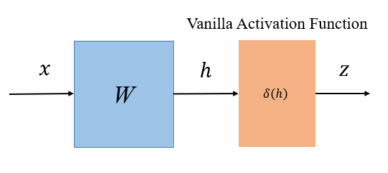
(a) Vanilla Activation Function

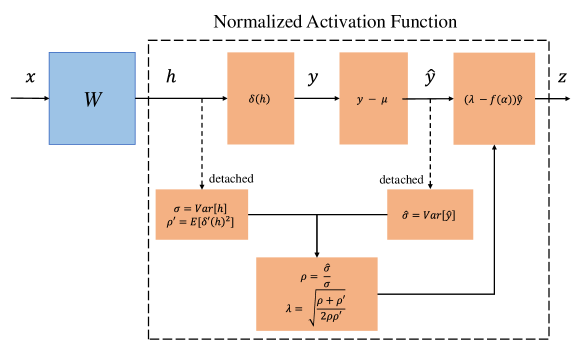
(b) Normalized Activation Function

Figure 1: The upper panel and the lower panel are two different activation function architectures we compare: (a) Vanilla Activation Function (b) Normalized Activation Function

At present, we can give the formula of our approach to normalize $\rho$ and $\rho^{\prime}$ for given activation function $\delta$:

$$\hat{\delta}\left(x\right)= \left(\lambda+f\left(\alpha\right)\right)\left(\delta\left(x\right)-\mu\right)$$ (15)

where $\mu$ is the expectation of $\delta\left(x\right)$; $\lambda$ denotes the normalization factor; $f$ is a bounded function to adjust $\lambda$; $\alpha$ is a learnable parameter. We call $\hat{\delta}\left(x\right)$ the normalized activation function. In this paper, we use $f\left(\alpha\right)=0.3\mathrm{Tanh}\left(\alpha\right)$ and $\alpha=0$ as initialization in all experiments.

In order to control the noise, $\rho$, $\rho^{\prime}$ and $\mu$ are updated by a momentum parameter $m$ based on history and current mini-batch. And they are also filtered out abnormal values out of bounds with two hyperparameters $L$ and $U$. The updating calculation can be described as the following:

$$\mu^{(t)}= m\mu_{M}+(1-m)\mu^{(t-1)}$$ (16)

$$\rho^{(t)}= \left\{\begin{aligned} \rho_{M},&\mbox{if }t=0\\ m\rho_{M}+(1-m)\rho^{(t-1)},&\mbox{if }L\rho^{(t-1)}<\rho_{M}<U\rho^{(t-1)}\\ \rho^{t-1},&\mbox{otherwise }\\ \end{aligned}\right.$$ (17)

$$\rho^{\prime(t)}= \left\{\begin{aligned} \rho^{\prime}_{M},&\mbox{if }t=0\\ m\rho^{\prime}_{M}+(1-m)\rho^{\prime(t-1)},&\mbox{if }L\rho^{\prime(t-1)}<\rho^{\prime}_{M}<U\rho^{\prime(t-1)}\\ \rho^{\prime(t-1)},&\mbox{otherwise }\\ \end{aligned}\right.$$ (18)

where $t$ denotes the number of batches (or iterations).

Note that $\rho$, $\rho^{\prime}$ and $\mu$ are obtained without gradient calculation. It means they are treated as three constants during backward-propagation. Therefore, this setting bypasses the problem of blocking the first and second derivatives of the loss that batch normalization operation suffers from (Zhou et al., 2022).

As a result that $x$ can be roughly guaranteed zero-mean as the assumption, we evaluated several prevalent activation functions by analytically calculating $\mathcal{R}$ score defined below.

$$\mathcal{R}_{x\sim\mathcal{N}\left(0,\sigma\right)}\left(\delta,\sigma\right) =\ln\frac{\mathbb{E}\left[\delta(x)^{2}\right]-\mathbb{E}\left[\delta(x)\right]^{2}}{\mathrm{Var}\left[x\right]\mathbb{E}\left[\left(\frac{\partial\delta\left(x\right)}{\partial x}\right)^{2}\right]}$$ (19)

$$\ =\ln\frac{\int_{-\infty}^{\infty}{\delta^{2}(x)\omega(x)\mathrm{d}x}-\frac{1}{\sigma\sqrt{2\pi}}\left(\int_{-\infty}^{\infty}{\delta(x)\omega(x)\mathrm{d}x}\right)^{2}}{\sigma^{2}\int_{-\infty}^{\infty}{\left(\frac{\partial\delta(x)}{\partial x}\right)^{2}\omega(x)\mathrm{d}x}}$$ (20)

$$\omega\left(x\right) =\exp\left(-\frac{x^{2}}{2\sigma^{2}}\right)$$ (21)

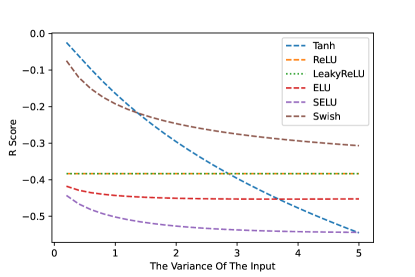
Figure 2: As shown above, the $\mathcal{R}$ score of common activation functions are constantly below 0. The $\mathcal{R}$ score of Tanh and Swish is desirably near 0 when the variance of input is small. However, they suffer from pseudo-linearity (Philipp et al., 2018) at the same time. The $\mathcal{R}$ score of ReLU and LeakyReLU are fixed at -0.383. Data are calculated with Mathematica.

In a normalized activation function, $\rho$ and $\rho^{\prime}$ can be normalized to be approximately around 1. Namely, property (i) is approached. Nonetheless, prevalent activation functions fail to achieve property (ii) as shown in figure 2. You may ask whether we can find a nonlinear activation function of which $\mathcal{R}$ converges to 0 and the post-activation is zero-mean. The answer is no. Lu et al. (2020) has proven it when the input is standard Gaussian. We further generalize their conclusion to any zero-mean Gaussian distribution and detailedly prove the following proposition in Appendix.

Proposition: Assume $x\sim\mathcal{N}\left(0,\sigma\right)$ and function $\delta:\mathbb{R}\rightarrow\mathbb{R}$ , then $\mathbb{E}\left[\delta\left(x\right)\right]=0$ and $\frac{\mathbb{E}\left[\delta\left(x\right)^{2}\right]}{\sigma^{2}}=\mathbb{E}\left[\delta^{\prime}\left(x\right)^{2}\right]=C$ if and only if $\delta\left(x\right)=\pm\sqrt{C}x$.

3 Experiments

With several experiments, we validate the effectiveness and advantage of our approach and investigate its compatibility with BN and residual networks. We benchmark NReLU (normalized ReLU) and NSwish (normalized Swish) against common activation functions, especially their unnormalized counterparts, as baselines. For convenience, we call a convolutional/linear layer plus the following BN and activation function a super-layer as a whole in this section.

All activation functions we compare are listed in Appendix.

3.1 LeNet5

First, we compare NReLU and NSwish against all baseline activation functions on LeNet5 using MNIST as the dataset. We run experiments in 50 epochs 25 times for each activation function and use the same learning rate with SGD. Networks using Tanh, NReLU and NSwish are initialized with Xavier initialization; ReLU, LReLU, ELU (Clevert et al., 2016), SELU (Klambauer et al., 2017) and Swish (Hendrycks & Gimpel, 2016; Ramachandran et al., 2018) with He initialization; ReLU-GPN (Lu et al., 2020) with orthogonal initialization (Saxe et al., 2014). We compare the mean and median of the accuracy and the number of models that fail to reach 98% validation accuracy until the 5-th, 10-th, 15-th, 30-th and 50-th epoch. Results are shown in Table 1.

Table 1: The table shows the best validation accuracy of different activation functions and the number of models that fail to reach 98% validation accuracy until different epochs. The best method among unnormalized/GPN/normalized versions is marked with “*”.

	validation accuracy		n models under 98% accuracy until i-th epoch
method	mean	median	5-th	10-th	15-th	30-th	50-th
Tanh	98.83	98.83	25	9	0	0	0
LReLU	98.87	98.87	25	4	0	0	0
ELU	98.90	98.90	23	0	0	0	0
SELU	98.90	98.91	9	0	0	0	0
ReLU	94.42	98.92	19	15	14	11	11
ReLU-GPN	87.50	98.91	14	7	6	5	5
NReLU	98.95*	98.96*	0	0	0	0	0
Swish	98.86	98.85	25	16	0	0	0
NSwish	98.90*	98.90*	1	0	0	0	0

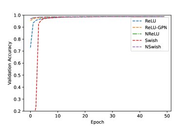
(a)

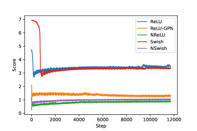
(b)

Figure 3: The left figure shows the increasing validation accuracy.The right figure illustrates the scores that we defined in Eq 22. Each curve is the median of 25 runs.

Then, we validate how the relation between $\rho$ and $\rho^{\prime}$ affects the convergence. Namely, how activation functions in a network satisfy property (i) influences the speed of convergence to some extent.

We recorded the $\rho$ and $\rho^{\prime}$ during training and compare the score defined below among different methods.

$$\ Score=\sum_{i=1}^{N}\frac{\lvert\ln\rho_{i}\rvert+\lvert\ln\rho_{i}^{\prime}\rvert}{2}$$ (22)

By comparison, We find that this score is roughly inversely related to the speed of convergence. We plot the accuracy and scores in Figure 3. It embodies the impact of activation functions on convergence we mentioned in section 2.1.

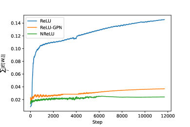
(a)

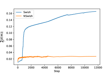
(b)

Figure 4: We recorded $\sum_{i}^{N}\left|\mathbb{E}{\bm{W}}_{i}\right|$ during training. The curves are the median of 25 runs.

We also monitored the mean of weight matrices. The result in Figure 4 shows our approach can inhibit weight matrices to shift from zero mean.

3.2 VGG

We benchmark our method on VGG19 (Simonyan & Zisserman, 2015) with CIFAR-100 dataset (Krizhevsky et al., 2009). We replaced ReLU with all activation functions we compare and train for 200 epochs. Super-layers using Tanh, NReLU, NLReLU and NSwish are initialized with Xavier initialization; ReLU, LReLU, ELU, SELU and Swish with He initialization; ReLU-GPN and LReLU-GPN with orthogonal initialization. We follow the same learning rate with AdamW (Loshchilov & Hutter, 2019). For networks using normalized activation functions, we use their unnormalized version as top three activation functions so that we need not change the model architecture and we remove affine transformation in BN followed by a normalized activation function.

	Top-1 Acc. (%)	Top-5 Acc. (%)
Tanh	25.63	55.50
LReLU	65.65	84.69
ELU	59.92	85.13
ReLU	65.65	85.50
NReLU	66.11	87.13
Swish	64.05	85.93
NSwish	65.72	87.40

Table 2: Comparing activation functions on CIFAR-100 dataset using VGG19 as backbone by reporting the median of 3 runs.

figureValidation accuracy of VGG19 on CIFAR-100. All curves are the median of 3 runs.

The results in Table 3 show our approach consistently outperforms its unnormalized counterparts, particularly in terms of top-5 accuracy. NSwish outperforms Swish by a 1.7% in terms of top1-accuracy.

Our approach makes the gradient on weights less easy to vanish when the network is enough deep so that it improves the trainability of neural networks. The operation of the normalized activation function is similar to BN (batch normalization) operation containing a scale and a shift. Intuitively, we wonder whether these similar operations mutually deteriorate effectiveness. In this experiment, we empirically testify that BN works well with normalized activation functions.

We find there are two key points when normalized activation functions are used with BN in this experiment.

• If we use BN right before normalized activation function, BN without affine transformation will be preferable, whereas removing affine transformation from the super-layer using an unnormalized activation function slightly degenerates the performance. We consider the reason is the affine transformation impairs the effort that BN tries to stabilize the zero-mean assumption and the variance of pre-activation.

• It is suggested to use a BN layer between the highest layer using normalized activation function and the top layer as a buffer, typically when normalized activation function is used with BN in lower layers. The reason we consider is that normalized activation function tries to keep the variance of output as the input which is not necessarily same as the variance of the target distribution. This buffer BN can prevent lower layers to raise the variance of output due to the increasing distance among classes during training and thus the moderate change of the variance gives rise to the relatively stable normalization factor.

The first point enables us to use fewer parameters, however, to achieve better performance.

Table 3: Validation accuracy of VGG19 without BN on CIFAR-100 across the 3 runs ordered by top-1 accuracy.

	Top-1 Acc.			Top-5 Acc.
SELU	64.49	64.16	63.83	87.28	87.31	87.07
ReLU-GPN	64.03	63.78	63.40	86.04	86.29	86.31
NReLU	67.28	66.31	66.02	87.65	88.00	88.15
LReLU-GPN	64.09	63.73	63.28	86.03	85.87	86.06
NLReLU	66.33	66.22	66.06	88.09	88.42	87.89
NSwish	64.66	63.19	63.15	85.49	85.47	86.21

For SELU, ReLU-GPN and LReLU-GPN, we run experiments using a learning rate of 0.01 with SGD and decay the learning rate by a factor of 0.2 every 60 epochs since the original optimizer did not converge. Given that SELU, ReLU-GPN and LReLU-GPN are proposed to be used without BN, we remove all BN layers in VGG and compare them with normalized activation functions working without BN. We additionally tested the NLReLU (normalized LeakyReLU) for comparing with LReLU-GPN.

3.3 ResNet

We also compared normalized activation function to other methods on ResNet with CIFAR-100 and Tiny ImageNet - a subset of ImageNet (Russakovsky et al., 2015). Due to the computational limitation, we choose the ResNet50 as the backbone. We follow the same set up and train for a fixed number of epochs, which can ensure the sufficient convergence of baselines.

For normalized activation functions, we replaced all activation functions which is not following the element-wise addition in the bottleneck with their normalized version, since the shift operation will decrease the ratio of positive elements in output and the variance of output will grow exponentially as the information flows to the deep block due to the scale operation, which will lead to extremely unstable normalization factor, if we use normalized activation function right after the element-wise addition. The unnormalized activation function lowers the variance of the output raised by the element-wise addition, whereas the normalized activation function keeps the variance and thus raises it exponentially as residual networks can be unraveled as hierarchical ensembles of relatively shallow networks (Veit et al., 2016).

We show the block for normalized activation function and unnormalized version in Appendix.

	Top-1 Acc.			Top-5 Acc.
Tanh	61.47	61.16	61.25	86.41	85.93	86.24
LReLU	71.13	70.33	70.01	91.40	90.63	91.07
ELU	72.10	71.96	71.82	92.03	91.89	91.75
SELU	69.05	68.80	68.37	90.35	90.42	90.42
ReLU	70.23	70.19	69.90	90.98	91.02	90.80
NReLU	71.63	71.38	70.99	91.72	91.51	91.38
Swish	71.71	71.60	71.16	91.54	91.51	91.44
NSwish	73.17	72.83	72.72	92.15	92.18	92.25

	Top-1 Acc.	Top-5 Acc.
Tanh	40.50	66.88
LReLU	54.90	78.20
ELU	54.06	77.67
SELU	48.66	74.18
ReLU	54.46	77.77
NReLU	56.01	78.99
Swish	54.93	78.39
NSwish	56.55	79.25

Table 4: Validation accuracy of ResNet50 on CIFAR-100 across the 3 runs.

Table 5: Comparing the median of validation accuracy on Tiny ImangeNet across 3 runs.

As the result shown in Table 5 and 5, NSwish outperforms Swish by nontrivial 1.4% at least on Tiny ImageNet and 1.2% on CIFAR-100. And NReLU outperforms ReLU by 1.1% at least on Tiny ImageNet and 1.0% on CIFAR-100. At the same time, the total number of trainable parameters of the normalized model is 15K fewer than the unnormalized one.

3.4 Natural Language Processing

We benchmark our approach on IMDb dataset (Maas et al., 2011) using TextRCNN (Lai et al., 2015). We train each network 5 times with the same set up from scratch, and the median validation accuracy is 90.2% for NReLU against 89.3% for ReLU, 90.1% for NSwish against 89.4% for Swish.

We also benchmark our method on the domain of machine translation. We train Transformer (Vaswani et al., 2017) models initialized with DeepNorm (Wang et al., 2022) on IWSLT 2015 De-En dataset and evaluate them on test set with standard BLEU metric. Higher layers tend to have smaller variance of the output signal of the residual funtion in a network with residual connections (He et al., 2016). Typically, the variance of the residual function output shrinks by the activation function from a relatively lower layer when the linear layer in FFN is broader, since a single layer has more poweful representation. At the same time, the normalized activation function recover the variance of post-activation which is originally supposed to be reduced by the activation function in a high FFN. Given that, we additionally train models where unnormalized activation functions are kept in the top k FFN of the encoder and decoder. We show the result in Appendix. Normalized activation function will prevent the residual function to have smaller magnitude if it is used in higher layers. However, it more thoroughly exploits the potential representational capacity of lower layers. Note that, in this experiment, $\lambda$ and $\mu$ are obtained with the instance-wise variance and mean.

4 Discussion

We have three tips for using normalized activation function with BN and in residual networks, which we have talked about detailedly in section 3.

• If we use BN right before normalized activation function, BN without affine transformation will be preferable.

• We suggest using a BN layer between the highest layer using normalized activation function and the top layer as a buffer when normalized activation function is used with BN in lower layers.

• When normalized activation function is applied in residual networks, we suggest to not replacing the unnormalized activation functions right after the element-wise addition in each block.

5 Conclusion

We propose a theoretically sound approach to normalize activation function. Then by carrying on several experiments, we empirically conclude that NReLU and NSwish consistently surpass the accuracy of their unnormalized version and at least one of them can outperform other activation functions, even with fewer parameters if BN is applied.

Appendix A Appendix

A.1 Activation Functions to Compare

• Tanh:

  $$f(x)=\frac{\exp(x)-\exp(-x)}{\exp(x)+\exp(-x)}$$ (23)

• ReLU:

  $$f(x) =\left\{\begin{aligned} x,&\mbox{if }x>0\\ 0,&\mbox{if }x\leq 0\end{aligned}\right.$$ (24)

• ReLU-GPN:

  $$f(x) =\beta\left\{\begin{aligned} x,&\mbox{if }x>0\\ 0,&\mbox{if }x\leq 0\end{aligned}\right.$$ (25)

  where $\beta\approx 1.4142$.

• LeakyReLU:

  $$f(x) =\left\{\begin{aligned} x,&\mbox{if }x>0\\ \alpha x,&\mbox{if }x\leq 0\end{aligned}\right.$$ (26)

  where $\alpha=0.01$.

• LeakyReLU-GPN:

  $$f(x) =\beta\left\{\begin{aligned} x,&\mbox{if }x>0\\ \alpha x,&\mbox{if }x\leq 0\end{aligned}\right.$$ (27)

  where $\alpha=0.01$; $\beta\approx 1.4141$.

• ELU:

  $$f(x) =\left\{\begin{aligned} x,&\mbox{if }x>0\\ \alpha(\exp(x)-1),&\mbox{if }x\leq 0\end{aligned}\right.$$ (28)

  where $\alpha=1.0$.

• SELU:

  $$f(x) =\lambda\left\{\begin{aligned} x,&\mbox{if }x>0\\ \alpha(\exp(x)-1),&\mbox{if }x\leq 0\end{aligned}\right.$$ (29)

  where $\alpha\approx 1.6733$; $\beta\approx 1.0507$.

• Swish:

  $$f(x)=\frac{x}{1+\exp(-x)}$$ (30)

Before we introduce normalized activation functions, let us predefine the following in order to avoid duplication:

$$\rho =\frac{\mathrm{Var}[y]}{\mathrm{Var}[x]}$$ (31)

$$\lambda =\sqrt{\frac{\rho+\rho^{\prime}}{2\rho\rho^{\prime}}}$$ (32)

where $x$ denotes the preactivation; $y$ denotes the output of the unnormalized activation function. The definition of $\rho^{\prime}$ is dependent on the unnormalized activation function and we define them differently in the following parts.

• NReLU(Normalized ReLU) is defined as

  $$f(x_{i}) =\left(\lambda+\beta\mathrm{Tanh}(\alpha)\right)\left(y_{i}-\bar{y}\right)$$ (33)

  $$y_{i} =\left\{\begin{aligned} x_{i},&\mbox{if }x>0\\ 0,&\mbox{if }x\leq 0\end{aligned}\right.$$ (34)

  $$\rho^{\prime} =P\left(x>0\right)$$ (35)

  Note that, the elements of the derivative of ReLU can be thought as a random variable following $Bernoulli(p)$ where $p$ is the ratio of positive elements in $x$. We take advantage of this property when talking about it working with the residual connection.

  The gradient of $\alpha$ can be easily derived from the chain rule.

  $$\frac{\partial Loss}{\partial\alpha} =\sum_{i}\beta\left(y_{i}-\bar{y}\right)\left(1-\mathrm{Tanh}(\alpha)^{2}\right)$$ (36)

  where $\sum_{i}$ runs over all positions of the feature map. We also need to compute the gradient with respect to the input feature map during training as following

  $$\frac{\partial Loss}{\partial x_{i}} =\left\{\begin{aligned} \lambda+\beta\mathrm{Tanh}(\alpha),&\mbox{if }x_{i}>0\\ 0,&\mbox{if }x_{i}\leq 0\end{aligned}\right.$$ (37)

• NSwish(Normalized Swish) is defined as

  $$f(x_{i}) =\left(\lambda+\beta\mathrm{Tanh}(\alpha)\right)\left(y_{i}-\bar{y}\right)$$ (38)

  $$y_{i} =x_{i}\mathrm{Sigmoid}(x_{i})$$ (39)

  $$\rho^{\prime} =\mathbb{E}\left[\left(y+x\mathrm{Sigmoid}(x)\left(1-y\right)\right)^{2}\right]$$ (40)

  For reason that Swish is a ReLU-like activation function, we also can roughly deem the elements of its derivative as a random variable following $Bernoulli(p)$. The gradient w.r.t. the parameter and the input feature map during training can be derived as:

  $$\frac{\partial Loss}{\partial\alpha} =\sum_{i}\beta\left(y_{i}-\bar{y}\right)\left(1-\mathrm{Tanh}(\alpha)^{2}\right)$$ (41)

  $$\frac{\partial Loss}{\partial x_{i}} =\left(\lambda+\beta\mathrm{Tanh}(\alpha)\right)\left(y+x\mathrm{Sigmoid}(x)\left(1-y\right)\right)$$ (42)

A.2 Proof

Proposition: Assume $x\sim\mathcal{N}\left(0,\sigma\right)$ and function $\delta:\mathbb{R}\rightarrow\mathbb{R}$ , then $\mathbb{E}\left[\delta\left(x\right)\right]=0$ and $\frac{\mathbb{E}\left[\delta\left(x\right)^{2}\right]}{\sigma^{2}}=\mathbb{E}\left[\delta^{\prime}\left(x\right)^{2}\right]=C$ if and only if $\delta\left(x\right)=\pm\sqrt{C}x$.

Proof. Let Hermite polynomials of $k$ degree be:

$$H_{k}(x) =\frac{(-1)^{k}}{\sqrt{k!}}\exp\left(\frac{x^{2}}{2\sigma^{2}}\right)\frac{d^{k}}{dx^{k}}\exp\left(-\frac{x^{2}}{2\sigma^{2}}\right)$$ (43)

Then we can derive that

$$\int_{-\infty}^{\infty}H_{k}(x)H_{j}(x)\exp(-\frac{x^{2}}{2\sigma^{2}}) =\left\{\begin{aligned} \sqrt{2\pi}\sigma^{-(2k-1)},&\mbox{if }k=j\\ 0,&\mbox{if }k\neq j\end{aligned}\right.$$ (44)

$$\int_{-\infty}^{\infty}H^{\prime}_{k}(x)H^{\prime}_{j}(x)\exp(-\frac{x^{2}}{2\sigma^{2}}) =\left\{\begin{aligned} k\sqrt{2\pi}\sigma^{-(2k+1)},&\mbox{if }k=j\\ 0,&\mbox{if }k\neq j\end{aligned}\right.$$ (45)

Since $\mathbb{E}_{x\sim\mathcal{N}\left(0,\sigma\right)}\left[\delta\left(x\right)^{2}\right]<\infty$; $\mathbb{E}_{{\textnormal{x}}\sim\mathcal{N}\left(0,\sigma\right)}\left[\delta^{\prime}\left(x\right)^{2}\right]<\infty$ and $\delta\left(x\right)$ and $\delta^{\prime}\left(x\right)$ can be expanded in terms of Hermite polynomials, we have

$$\delta(x) =\sum_{k=0}^{\infty}a_{k}H_{k}(x)$$ (46)

$$\delta^{\prime}(x) =\sum_{k=1}^{\infty}a_{k}H^{\prime}_{k}(x)$$ (47)

Due to $\mathbb{E}_{x\sim\mathcal{N}\left(0,\sigma\right)}\left[\delta\left(x\right)\right]=0$, we have

$$a_{0}=0$$ (48)

According to Equation 44, 45 and

$$\frac{\mathbb{E}\left[\delta\left(x\right)^{2}\right]}{\sigma^{2}}=\mathbb{E}\left[\delta^{\prime}\left(x\right)^{2}\right]=C$$ (49)

we have

$$\frac{\mathbb{E}\left[\delta\left(x\right)^{2}\right]}{\sigma^{2}}=\frac{1}{\sigma^{2}}\sum_{k=1}^{\infty}\sigma^{-2k}a_{k}^{2}=\mathbb{E}\left[\delta^{\prime}\left(x\right)^{2}\right]=\sum_{k=1}^{\infty}k\sigma^{-2k-2}a_{k}^{2}=C$$ (50)

Thus we can derive that

$$\sum_{k=1}^{\infty}k\sigma^{-2(k+1)}a_{k}^{2}-\sum_{k=1}^{\infty}\sigma^{-2(k+1)}a_{k}^{2}=0$$ (51)

that is

$$\sum_{k=2}^{\infty}(k-1)\sigma^{-2(k+1)}a_{k}^{2}=0$$ (52)

For the reason that all terms in $\sum_{k=2}^{\infty}(k-1)\sigma^{-2(k+1)}a_{k}^{2}$ is nonnegative, the only solution is $a_{k}=0$ for all $k\geq 2$. And for $\mathbb{E}\left[\delta^{\prime}\left(x\right)^{2}\right]=\sigma^{-4}a_{1}^{2}=C$, we have $a_{1}=\pm\sigma^{2}\sqrt{C}$. Hence $\delta(x)=\pm\sqrt{C}x$.

This proof is largely based on Lu et al. (2020) with minor generalization here.

A.3 Block for ResNet50

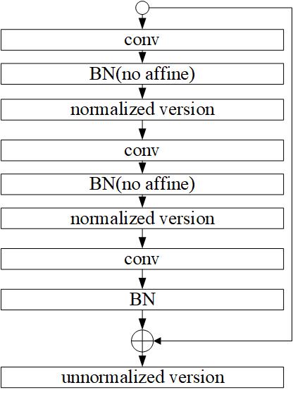
(a)

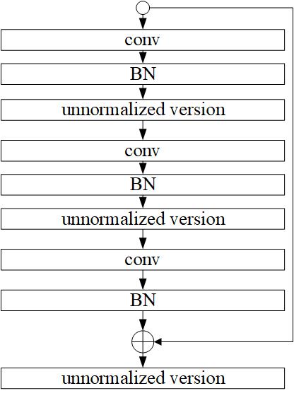
(b)

Figure 5: Left: a block for normalized activation function.Right: a block for unnormalized activation function.

A.4 Results And Hyperparamters

Table 6: The BLEU points of 12L-12L Transformer on IWSLT 2015 across different hyperparameter settings. NSwish+$k$Swish denotes that the model uses normalized activation functions as the unnormalized ones are kept in the top $k$ FFN of the encoder and decoder. BLEU scores in parenthesis are calculated with sentences translated with a beam size of 5. The rest experiments are still training at the time of submission.

	the size of the first layer in FNN
	512 * 512	512 * 1024	512 * 2048
Swish	28.38(29.50)	29.27(30.31)	29.38(30.52)
NSwish	26.78(27.91)	13.54(14.58)	11.05(12.98)
NSwish+1Swish	29.06(30.44)	29.38(30.17)	11.43(12.91)
NSwish+6Swish	-	-	29.37(30.61)

Table 7: The BLEU points of 6L-6L Transformer on IWSLT 2015 with different hyperparameter settings. BLEU scores in parenthesis are calculated with sentences translated with a beam size of 5. The score with an italic font is the median BLEU of 3 runs. The rest experiments are still training at the time of submission.

	the size of the first layer in FNN
	512 * 512	512 * 1024	512 * 2048
ReLU	27.69(28.72)	27.81(28.92)	28.80(29.75)
NReLU+1ReLU	27.93(28.81)	27.91(29.17)	-
NReLU+3ReLU	27.64(28.82)	-	29.37(30.43)

Table 8: The hyperparameter setting for the experiment on VGG19 and ResNet50. Our method works well without warmup as well.

Hyperparameters	Value
Learning Rate	1e-3
Batch Size	128
Training Epochs	200
Warmup Updates	first epoch
Dropout	0.5
Gradient Clipping	3.0

Table 9: The hyperparameter setting for the experiment on machine translation comparing Swish and Nswish.

Hyperparameters	Value
Learning Rate	5e-4
Batch Size	128
Training Epochs	20
Warmup Updates	4000
Dropout	0.5
Gradient Clipping	3.0
Training Max Length	50

Table 10: The hyperparameter setting for the experiment on machine translation comparing ReLU and NReLU.

Hyperparameters	Value
Learning Rate	5e-4
Batch Size	256
Training Epochs	20
Warmup Updates	4000
Dropout	0.5
Gradient Clipping	3.0
Training Max Length	50

References

- Clevert et al. (2016) Djork-Arné Clevert, Thomas Unterthiner, and Sepp Hochreiter. Fast and accurate deep network learning by exponential linear units (elus). In Yoshua Bengio and Yann LeCun (eds.), 4th International Conference on Learning Representations, ICLR 2016, San Juan, Puerto Rico, May 2-4, 2016, Conference Track Proceedings, 2016.
- Devlin et al. (2019) Jacob Devlin, Ming-Wei Chang, Kenton Lee, and Kristina Toutanova. BERT: pre-training of deep bidirectional transformers for language understanding. In Jill Burstein, Christy Doran, and Thamar Solorio (eds.), Proceedings of the 2019 Conference of the North American Chapter of the Association for Computational Linguistics: Human Language Technologies, NAACL-HLT 2019, Minneapolis, MN, USA, June 2-7, 2019, Volume 1 (Long and Short Papers), pp. 4171–4186. Association for Computational Linguistics, 2019. doi: 10.18653/v1/n19-1423.
- Glorot & Bengio (2010) Xavier Glorot and Y. Bengio. Understanding the difficulty of training deep feedforward neural networks. Journal of Machine Learning Research - Proceedings Track, 9:249–256, 01 2010.
- He et al. (2015) Kaiming He, Xiangyu Zhang, Shaoqing Ren, and Jian Sun. Delving deep into rectifiers: Surpassing human-level performance on imagenet classification. IEEE International Conference on Computer Vision (ICCV 2015), 1502, 02 2015. doi: 10.1109/ICCV.2015.123.
- He et al. (2016) Kaiming He, Xiangyu Zhang, Shaoqing Ren, and Jian Sun. Deep residual learning for image recognition. In 2016 IEEE Conference on Computer Vision and Pattern Recognition, CVPR 2016, Las Vegas, NV, USA, June 27-30, 2016, pp. 770–778. IEEE Computer Society, 2016. doi: 10.1109/CVPR.2016.90.
- Hendrycks & Gimpel (2016) Dan Hendrycks and Kevin Gimpel. Gaussian error linear units (gelus). arXiv preprint arXiv:1606.08415, 2016.
- Ioffe & Szegedy (2015) Sergey Ioffe and Christian Szegedy. Batch normalization: Accelerating deep network training by reducing internal covariate shift. In Francis R. Bach and David M. Blei (eds.), Proceedings of the 32nd International Conference on Machine Learning, ICML 2015, Lille, France, 6-11 July 2015, volume 37 of JMLR Workshop and Conference Proceedings, pp. 448–456. JMLR.org, 2015.
- Klambauer et al. (2017) Günter Klambauer, Thomas Unterthiner, Andreas Mayr, and Sepp Hochreiter. Self-normalizing neural networks. In Isabelle Guyon, Ulrike von Luxburg, Samy Bengio, Hanna M. Wallach, Rob Fergus, S. V. N. Vishwanathan, and Roman Garnett (eds.), Advances in Neural Information Processing Systems 30: Annual Conference on Neural Information Processing Systems 2017, December 4-9, 2017, Long Beach, CA, USA, pp. 971–980, 2017.
- Krähenbühl et al. (2016) Philipp Krähenbühl, Carl Doersch, Jeff Donahue, and Trevor Darrell. Data-dependent initializations of convolutional neural networks. In Yoshua Bengio and Yann LeCun (eds.), 4th International Conference on Learning Representations, ICLR 2016, San Juan, Puerto Rico, May 2-4, 2016, Conference Track Proceedings, 2016.
- Krizhevsky et al. (2009) Alex Krizhevsky, Geoffrey Hinton, et al. Learning multiple layers of features from tiny images. 2009.
- Krizhevsky et al. (2012) Alex Krizhevsky, Ilya Sutskever, and Geoffrey E. Hinton. Imagenet classification with deep convolutional neural networks. In Peter L. Bartlett, Fernando C. N. Pereira, Christopher J. C. Burges, Léon Bottou, and Kilian Q. Weinberger (eds.), Advances in Neural Information Processing Systems 25: 26th Annual Conference on Neural Information Processing Systems 2012. Proceedings of a meeting held December 3-6, 2012, Lake Tahoe, Nevada, United States, pp. 1106–1114, 2012.
- Lai et al. (2015) Siwei Lai, Liheng Xu, Kang Liu, and Jun Zhao. Recurrent convolutional neural networks for text classification. In Blai Bonet and Sven Koenig (eds.), Proceedings of the Twenty-Ninth AAAI Conference on Artificial Intelligence, January 25-30, 2015, Austin, Texas, USA, pp. 2267–2273. AAAI Press, 2015.
- Loshchilov & Hutter (2019) Ilya Loshchilov and Frank Hutter. Decoupled weight decay regularization. In 7th International Conference on Learning Representations, ICLR 2019, New Orleans, LA, USA, May 6-9, 2019. OpenReview.net, 2019.
- Lu et al. (2020) Yao Lu, Stephen Gould, and Thalaiyasingam Ajanthan. Bidirectional self-normalizing neural networks. CoRR, abs/2006.12169, 2020. URL https://arxiv.org/abs/2006.12169.
- Maas et al. (2011) Andrew L. Maas, Raymond E. Daly, Peter T. Pham, Dan Huang, Andrew Y. Ng, and Christopher Potts. Learning word vectors for sentiment analysis. In Dekang Lin, Yuji Matsumoto, and Rada Mihalcea (eds.), The 49th Annual Meeting of the Association for Computational Linguistics: Human Language Technologies, Proceedings of the Conference, 19-24 June, 2011, Portland, Oregon, USA, pp. 142–150. The Association for Computer Linguistics, 2011.
- Philipp et al. (2018) George Philipp, Dawn Song, and Jaime G. Carbonell. Gradients explode - deep networks are shallow - resnet explained. In 6th International Conference on Learning Representations, ICLR 2018, Vancouver, BC, Canada, April 30 - May 3, 2018, Workshop Track Proceedings. OpenReview.net, 2018.
- Ramachandran et al. (2018) Prajit Ramachandran, Barret Zoph, and Quoc V. Le. Searching for activation functions. In 6th International Conference on Learning Representations, ICLR 2018, Vancouver, BC, Canada, April 30 - May 3, 2018, Workshop Track Proceedings. OpenReview.net, 2018.
- Russakovsky et al. (2015) Olga Russakovsky, Jia Deng, Hao Su, Jonathan Krause, Sanjeev Satheesh, Sean Ma, Zhiheng Huang, Andrej Karpathy, Aditya Khosla, Michael S. Bernstein, Alexander C. Berg, and Li Fei-Fei. Imagenet large scale visual recognition challenge. Int. J. Comput. Vis., 115(3):211–252, 2015. doi: 10.1007/s11263-015-0816-y.
- Saxe et al. (2014) Andrew M. Saxe, James L. McClelland, and Surya Ganguli. Exact solutions to the nonlinear dynamics of learning in deep linear neural networks. In Yoshua Bengio and Yann LeCun (eds.), 2nd International Conference on Learning Representations, ICLR 2014, Banff, AB, Canada, April 14-16, 2014, Conference Track Proceedings, 2014.
- Simonyan & Zisserman (2015) Karen Simonyan and Andrew Zisserman. Very deep convolutional networks for large-scale image recognition. In Yoshua Bengio and Yann LeCun (eds.), 3rd International Conference on Learning Representations, ICLR 2015, San Diego, CA, USA, May 7-9, 2015, Conference Track Proceedings, 2015.
- Srivastava et al. (2014) Nitish Srivastava, Geoffrey Hinton, Alex Krizhevsky, Ilya Sutskever, and Ruslan Salakhutdinov. Dropout: A simple way to prevent neural networks from overfitting. Journal of Machine Learning Research, 15(56):1929–1958, 2014.
- Vaswani et al. (2017) Ashish Vaswani, Noam Shazeer, Niki Parmar, Jakob Uszkoreit, Llion Jones, Aidan N. Gomez, Lukasz Kaiser, and Illia Polosukhin. Attention is all you need. In Isabelle Guyon, Ulrike von Luxburg, Samy Bengio, Hanna M. Wallach, Rob Fergus, S. V. N. Vishwanathan, and Roman Garnett (eds.), Advances in Neural Information Processing Systems 30: Annual Conference on Neural Information Processing Systems 2017, December 4-9, 2017, Long Beach, CA, USA, pp. 5998–6008, 2017.
- Veit et al. (2016) Andreas Veit, Michael Wilber, and Serge Belongie. Residual networks behave like ensembles of relatively shallow networks. Advances in Neural Information Processing Systems, 05 2016.
- Wang et al. (2022) Hongyu Wang, Shuming Ma, Li Dong, Shaohan Huang, Dongdong Zhang, and Furu Wei. Deepnet: Scaling transformers to 1, 000 layers. CoRR, abs/2203.00555, 2022. doi: 10.48550/arXiv.2203.00555. URL https://doi.org/10.48550/arXiv.2203.00555.
- Zhou et al. (2022) Zhanpeng Zhou, Wen Shen, Huixin Chen, Ling Tang, and Quanshi Zhang. Batch normalization is blind to the first and second derivatives of the loss. CoRR, abs/2205.15146, 2022. doi: 10.48550/arXiv.2205.15146. URL https://doi.org/10.48550/arXiv.2205.15146.