Meson resonance gas in a relativistic quark model:
scalar vs vector confinement and semishort range correlations

Relativistic quarks in a meson resonance gas:
scalar vs vector confinement and semishort range correlations

Abstract

Smooth transitions from hadronic matter to hot and dense matter of quantum chromodynamics accompany continuous transformations in effective degrees of freedom. The microscopic descriptions should include relativistic quarks interacting inside of hadrons. In this work we construct a schematic constituent quark model with relativistic kinematics which captures the global trends of meson spectra in the light, strange, and charm quark sectors. We examine the roles of the scalar- and vector-confining potentials as well as semishort range correlations in estimating the strength of central, spin-spin, and spin-orbit interactions. The quark dynamics in low-lying mesons is very sensitive to relativistic kinematics and short range interactions, while in high-lying mesons are sensitive to the composition of scalar- and vector-confinement. After expressing mesons in terms of quark wave functions, we use them to describe the quark occupation probability in a meson resonance gas, and discuss how it can be related to its counterpart in a quark-gluon-plasma.

I Introduction

Quarks and gluons in quantum chromodynamics (QCD) play multiple roles in hadron physics; they are not only constituents of hadrons, but also are mediators of hadron-hadron interactions ’t Hooft (1974); Witten (1979a); Fukushima et al. (2020). The quark exchanges are microscopic descriptions of traditional meson exchanges Yukawa (1935); Nambu (1957); Sakurai (1960); Stoks et al. (1994); Machleidt et al. (1996), and also can describe the baryon-baryon hard core repulsions at short distance Hatsuda (2018); Park et al. (2020); Oka and Yazaki (1980, 1981a, 1981b). When many hadrons are strongly interacting in a matter, hadrons are supposed to exchange substantial amount of quarks and gluons, and therefore it should be difficult to differentiate such strongly interacting hadronic matter from matters of quarks and gluons McLerran and Pisarski (2007); Masuda et al. (2013a); Kojo et al. (2015).

There are several circumstances where hadrons in a matter interact strongly. In a heated hadronic matter many hadron resonances are generated and begin to overlap around $T\sim 150$ MeV, and the matter smoothly transforms into a quark-gluon-plasma (QGP) through a crossover transition. Such crossover has been confirmed by lattice QCD simulations Aoki et al. (2006) and fluctuation analyses in heavy-ion collisions Abdallah et al. (2021). Another example of strongly interacting hadronic matter is a highly compressed nuclear matter in which nuclear many-body forces rapidly become important around twice nuclear saturation density Akmal et al. (1998); Gandolfi et al. (2012). The quark exchange picture of nuclear forces motivates the scenario of smooth transitions from nuclear to quark matter McLerran and Pisarski (2007); Masuda et al. (2013a); Kojo et al. (2015); Fukushima et al. (2020), which results in new qualitative features for equations of state such as the sound velocity peak in the crossover domain Masuda et al. (2013a, b); Kojo et al. (2015); Baym et al. (2018, 2019); Kojo et al. (2022); McLerran and Reddy (2019); Jeong et al. (2020); Duarte et al. (2020a, b); Kojo (2021a); Kojo and Suenaga (2022); Iida and Itou (2022). The interplay between nuclear and quark equations of state is one of the central issues in neutron star phenomenology Drischler et al. (2021); Kojo (2021b); Brandes et al. (2022); Gorda et al. (2022); Huang et al. (2022); Fujimoto et al. (2022); Marczenko et al. (2022).

The above mentioned examples involve changes in effective degrees of freedom from composite to elementary particles. In order to understand such transitions in QCD, it is crucial to study quark- and gluon-substructures of hadrons. In this work we analyze the meson spectra within a schematic quark model, following the spirit and methodology of traditional constituent quark models De Rujula et al. (1975); Eichten et al. (1978); Godfrey and Isgur (1985); Capstick and Isgur (1986); Schnitzer (1978); Ebert et al. (2009, 2010, 1998, 2002, 2011) which have successfully reproduced not only the spectra but also the widths and hadronic couplings. Our purpose here is to utilize some concepts and technology developed in the previous works and to present them in a schematic relativistic quark model. Technical complications found in the previous works are considerably simplified by semi-phenomenological treatments that in turn enable us flexible approaches to more complicated systems.

While this work does not have much improvement in reproducing hadronic quantities compared to the previous works De Rujula et al. (1975); Eichten et al. (1978); Godfrey and Isgur (1985); Capstick and Isgur (1986); Schnitzer (1978); Ebert et al. (2009, 1998, 2002, 2011), this work has more focus on the application to hadronic matter in which the structure of hadrons may change. In particular we manifestly present the sensitivity of hadronic spectra and structures to modeling in relativistic effects, short range correlations, and confining potentials. Such sensitivity may be obvious to experts working on quark models, but to the best of our knowledge is not much emphasized and is difficult to see from the outside of the community for the hadron spectroscopy. Since the effective model parameters for quark dynamics in a hadron may be influenced by hadron-hadron interactions, it is important to specify which properties of hadrons can be stable until hadrons substantially overlap.

We analyze the global features of mesons from the light to heavy quark sectors, reproducing the spectra better than $10\%$ level. We are particularly interested in the impacts of the relativistic kinematics Godfrey and Isgur (1985); Capstick and Isgur (1986), scalar- vs vector-confinement Schnitzer (1978); Ebert et al. (2009, 1998, 2002, 2011), and semishort range correlations mediated by one-gluon exchanges. All these effects are important especially in high density matter where particles become relativistic. The distinction between scalar- and vector-confinement is connected to the relation between the chiral restoration and confinement, as the scalar vertices in vacuum is enhanced by the chiral symmetry breaking Alkofer et al. (2008). The correlation between confinement and chiral symmetry breaking Casher (1979); Banks and Casher (1980); Coleman and Witten (1980) is relevant to the chiral symmetry breaking/restoration in hadron-to-quark matter transitions Hatsuda et al. (2006); Yamamoto et al. (2007); Glozman and Wagenbrunn (2008); Kojo et al. (2010a, 2012, b); Minamikawa et al. (2021).

As a quick application to hadronic matter under extreme conditions, we consider a meson gas at finite temperature and examine the quark contents. It has been known that a hadron resonance gas (HRG) model Venugopalan and Prakash (1992); Karsch et al. (2003a, b), where interactions among hadrons are neglected, reproduces the results of lattice Monte-Carlo calculations up to $\sim 150$ MeV quite well. In the context of HRG-QGP crossover, we are interested in how close quark contents in a HRG can be to those in a QGP. The quark momentum distribution in a given meson is used to study the quark momentum distribution in a hot HRG. A fuller examination of various quantities, e.g., chiral condensates, Polyakov loops, and so on, as well as the impacts of baryon resonances will be presented in separate publications.

This paper is organized as follows. In Sec. II we set up equations for bound state problems and explain how the relativistic kinematic factors are treated. In Sec. III we discuss the potentials including various quark vertices. In Sec. IV we examine meson spectra and constrain our model parameters through fitting. In Sec. V we calculate the single quark momentum distribution in a meson. In Sec. VI we calculate the quark occupation probabilities in a meson gas. Sec. VII is devoted to summary.

II Relativistic quark model

II.1 The relations to the previous works

As there are several successful constituent quark models which have strongly influenced our modeling, we first comment on the similarity and difference between our work and the previous studies.

Our discussions on the relativistic kinematics (to be presented shortly in Sec.II.2) are largely motivated from the seminal works by Ebert et al. Ebert et al. (2009, 1998, 2002, 2011) which took into account the relativistic kinematics, the mixture of scalar-vector confining potentials, and short range interactions. The model is able to reproduce the experimental spectra from light to bottom quark sectors quite well. The authors replaced the quark energies appearing in various relativistic factors with some sort of energy constants which depend on the meson masses under discussions. No expansion of quark momenta of $\sim{\bm{p}}/m$ is used. Our model applies similar simplifications to relativistic kinematic factors, but our usage is more intuitive; we simply replace quark momenta with its average which are self-consistently estimated. Our model adopts the mixture of scalar and vector confining potentials as in Refs.Ebert et al. (2009, 1998, 2002, 2011), but ours turn out to be dominated by the conventional scalar-type, while the latter by the vector-type. The anomalous color magnetic moment used in Refs.Ebert et al. (2009, 1998, 2002, 2011), which substantially complicates the whole analyses, is omitted in the present paper since we feel that introduction of such a term requires another justification and examination.

Another important work which we refer to is the work by Godfrey-Isgur for mesons Godfrey and Isgur (1985) and its extension to baryons Capstick and Isgur (1986). The authors treated the relativistic kinematics in a more complete manner than the averaging procedure in our modeling. The potentials contain the scalar confining potential, short range Coulomb term, and various spin dependent potentials, all of which are convoluted with some phenomenological smearing functions including the quark mass dependence. In our modeling, we do not directly use such smearing functions as we could not find simple reasonings for the parameterization. But we do refer to the physical considerations in Refs.Godfrey and Isgur (1985); Capstick and Isgur (1986) when we need to handle artificial singularities appearing in some short-range interactions. As a whole our parametrization of various effects is based on more intuitive and straightforward considerations than Refs.Godfrey and Isgur (1985); Capstick and Isgur (1986) and less sophisticated, but may be more flexible due to technical simplifcations. Finally, Refs.Godfrey and Isgur (1985); Capstick and Isgur (1986) treat $\alpha_{s}$ as space-dependent to express its running behavior including the IR domain, while we simply consider only typical values of $\alpha_{s}$ for given energy scales. After getting the list of $\alpha_{s}$ for good fits, we extract plausible trends of $\alpha_{s}$ in the infrared.

In short, we aim at modeling which is intermediate between very popular non-relativistic quark models De Rujula et al. (1975); Eichten et al. (1978) and more elaborated relativistic quark models in Refs.Godfrey and Isgur (1985); Capstick and Isgur (1986); Schnitzer (1978); Ebert et al. (2009, 1998, 2002, 2011). We believe that treatments at the level of resolutions in this work are useful for grasping the qualitative features of many-body systems; the advantage in our model is its intuitive feature which allows us to examine the correlation between the quark dynamics in a hadron and the properties of matter.

II.2 Basic equation

We compute a meson mass at rest and the corresponding wavefunction. We solve equations for relativistic quarks. Our starting point is ($\int_{\bm{q}}\equiv\int\mathrm{d}^{3}{\bm{q}}/(2\pi)^{3}$)

$$\big{[}M-E_{1}({\bm{p}})-E_{2}({\bm{p}})\big{]}\Psi({\bm{p}})=\int_{{\bf q}}V({\bm{p}},{\bm{q}})\Psi({\bm{q}})\,,$$ (1)

where $M$ is the meson mass, $E_{i=1,2}({\bm{p}})=\sqrt{{\bm{p}}^{2}+m_{i}^{2}}$ the energies of quarks 1 and 2, and $\Psi({\bm{p}})$ the meson wavefunction at rest. The two body effective potential $V({\bm{p}},{\bm{q}})$ includes the Dirac spinors and the matrix elements at the vertices. We take the center of mass frame of the two quarks, and ${\bm{p}}$, ${\bm{q}}$ are relative momenta (here the quark momenta are ${\bm{p}}_{1}=-{\bm{p}}_{2}={\bm{p}}$ or ${\bm{q}}$). $m_{i=1,2}$ are the constituent quark masses of $\sim 0.3$ GeV for light quarks, $\sim 0.5$ GeV for strange quarks, and $\sim 1.5$ GeV for charm quarks.

Following the approaches in Refs.Ebert et al. (2009, 1998, 2002, 2011), we rewrite Eq.(1) into a Schrödinger-type differential equation. This is possible even without applying the nonrelativistic expansion. We first multiply a factor

$$I_{M}({\bm{p}})=\frac{\,\big{[}M+E_{1}+E_{2}\big{]}\big{[}M^{2}-(E_{1}-E_{2})^{2}\big{]}\,}{4M^{2}}\,,$$ (2)

to Eq.(1), and obtain a Schödinger-like equation

$$\big{(}b_{M}-{\bm{p}}^{2}\big{)}\Psi({\bm{p}})=\int_{{\bm{q}}}\mathcal{V}_{M}({\bm{p}},{\bm{q}})\Psi({\bm{q}})\,,$$ (3)

where we wrote

$$\mathcal{V}_{M}({\bm{p}},{\bm{q}})\equiv I_{M}({\bm{p}})V({\bm{p}},{\bm{q}})\,,$$ (4)

and

$$b_{M}=\frac{\,\big{[}M^{2}-(m_{1}+m_{2})^{2}\big{]}\big{[}M^{2}-(m_{1}-m_{2})^{2}\big{]}\,}{4M^{2}}\,,$$ (5)

is a constant depending on the meson mass $M$.

Although the equation looks a usual eigenvalue equation, the actual determination of the meson mass $M$ is more complex because $M$ appears in kinematic factors in $\mathcal{V}_{M}$. To determine $M$, we find the eigenvalue $\lambda_{M}$ of an equation $\big{(}{\bm{p}}^{2}+\mathcal{V}_{M}\big{)}|\Psi\rangle=\lambda_{M}|\Psi\rangle$ for a given $M$, and check whether $\lambda_{M}$ coincides with $b_{M}$. Only the value $M$ satisfying $\lambda_{M}=b_{M}$ is adopted as a physical meson spectrum.

II.3 Averaging kinematic factors

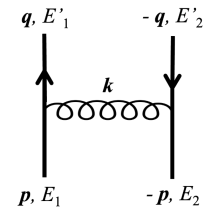
Figure 1: A graph for two-body scattering with the notations corresponding to those in the main text.

The effective potentials $\mathcal{V}_{M}({\bm{p}},{\bm{q}})$ in Eq.(11) contain various quark kinematic factors associated with the energies and spinors. In particular quark momenta can appear in denominators. To simplify the calculations we replace some of momenta with the average values for a given meson. First we rewrite $\mathcal{V}_{M}({\bm{p}},{\bm{q}})$ as a function of $E_{1,2}({\bm{p}})$ and $E^{\prime}_{1,2}({\bm{q}})$, the average momentum ${\bm{P}}$ before and after interactions (not total momentum!), and the momentum transfer ${\bm{k}}$ as

$${\bm{P}}=\frac{\,{\bm{p}}+{\bm{q}}\,}{2}\,,~{}~{}~{}{\bm{k}}={\bm{p}}-{\bm{q}}\,.$$ (6)

The potential can be expressed as

$$\mathcal{V}_{M}({\bm{p}},{\bm{q}})=\tilde{\mathcal{V}}_{M}(E_{1,2},E^{\prime}_{1,2};{\bm{P}},{\bm{k}})\,.$$ (7)

Here, for later convenience we wrote $E,E^{\prime}$ as if they are independent of ${\bm{P}},{\bm{k}}$.

Our approximation takes the time average of ${\bm{P}}^{2}$ which has a typical value for a given meson. We approximate the energies as

$$E_{i}({\bm{p}}),E^{\prime}_{i}({\bm{q}})~{}\rightarrow~{}\bar{E_{i}}=\sqrt{m_{i}^{2}+\bar{{\bm{P}}}^{2}}\,,$$ (8)

where $\bar{{\bm{P}}}^{2}$ is the average of ${\bm{P}}^{2}$. Next, if we encounter expressions such as $P_{i}$ or $P_{i}P_{j}$, we take the average as

$$P_{i}~{}\rightarrow~{}0\,,~{}~{}~{}P_{i}P_{j}~{}\rightarrow\delta_{ij}\bar{{\bm{P}}}^{2}/3\,.$$ (9)

and so on. With these procedures

$$\mathcal{V}_{M}({\bm{p}},{\bm{q}})~{}\rightarrow~{}\overline{\mathcal{V}}_{M,\bar{{\bm{P}}}^{2}}({\bm{k}})\,.$$ (10)

For this effective potential, the only variable is ${\bm{k}}$, and one can take the Fourier transform of Eq.(11) to obtain

$$b_{M}\Psi({\bm{r}})=\big{[}\,-\nabla^{2}+\overline{\mathcal{V}}_{M,\bar{{\bm{P}}}^{2}}({\bm{r}})\,\big{]}\Psi({\bm{r}})\,.$$ (11)

In practice, we substitute some values of $\bar{{\bm{P}}}^{2}$, find the eigenstates, and compute the expectation value $\langle{\bm{P}}^{2}\rangle$ to check whether our choice of $\bar{{\bm{P}}}^{2}$ coincides with $\langle{\bm{P}}^{2}\rangle$. This forms a self-consistent equation for a given $M$ (which does not necessarily give the solution, $\lambda_{M}=b_{M}$). In this work we varied $\bar{{\bm{P}}}^{2}$ with only grids of $0.01\,{\rm GeV}^{2}$ without demanding perfect consistency. The choice of $\bar{{\bm{P}}}^{2}$ depends on the potential and the state we are looking at. For example, if the potential for the equal quark mass case is the pure Coulomb type, then $\bar{{\bm{P}}}^{2}\sim(\alpha_{s}m)^{2}$, with which the non-relativistic approximation is valid only for $\alpha_{s}(m^{2})\ll 1$. The linear rising potential modifies this simple rule, but in general we found $|{\bm{P}}|$ is the order of $\gtrsim 0.3$ GeV $\sim\alpha_{s}(m_{u,d}^{2})m_{u,d}$ for light quarks and $\gtrsim 0.5$ GeV $\sim\alpha_{s}(m_{c}^{2})m_{c}$ for charm quarks.

There is a qualification on the above averaging procedures Eq.(9) for ${\bm{P}}$. We actually have dropped the appearance of some angular momentum operators which otherwise leave the ${\bm{L}}\cdot{\bm{S}}$ type operators. To correctly keep such terms, we add an extra rule here. When ${\bm{P}}$ appears in the combination of ${\bm{k}}\times{\bm{P}}$ together with the wavefunction $\Psi({\bm{q}})$, we use ${\bm{P}}={\bm{q}}+{\bm{k}}/2$ to rewrite ${\bm{k}}\times{\bm{P}}={\bm{k}}\times{\bm{q}}$. Taking the Fourier transform,

$$\int_{{\bm{p}},{\bm{q}}}\mathrm{e}^{\mathrm{i}{\bm{p}}\cdot{\bm{r}}}({\bm{k}}\times{\bm{q}})f({\bm{k}})\Psi({\bm{q}})=-{\bm{\nabla}}f({\bm{r}})\times{\bm{\nabla}}\Psi({\bm{r}})\,.$$ (12)

For a rotationally symmetric function $f({\bm{r}})=f(r)$,

$${\bm{\nabla}}f({\bm{r}})\times{\bm{\nabla}}\Psi({\bm{r}})=\frac{\,\partial_{r}f(r)\,}{\,r\,}{\bm{L}}\Psi({\bm{r}})\,,$$ (13)

with ${\bm{r}}\times{\bm{q}}={\bm{r}}_{1}\times{\bm{q}}+{\bm{r}}_{2}\times(-{\bm{q}})={\bm{l}}_{1}+{\bm{l}}_{2}={\bm{L}}$ being the total angular momentum operator acting on $\Psi$.

II.4 Several kinematic limits

Here we analyze various kinematic limits. We give a brief summary here for the factors given in Eqs.(2), (5), and the eigvenvalue equation Eq.(11).

For a heavy-heavy meson with $m_{1}=m_{2}=m_{h}$, the kinematic factor is $(M\sim 2m_{h})$

$$I_{M}^{hh}\simeq\frac{\,M+2m_{h}\,}{4}\simeq m_{h}\,,$$ (14)

and

$$b_{M}^{hh}=M-2m_{h}\,.$$ (15)

With the potential $\bar{V}^{hh}=\bar{V}_{m_{1},m_{2}\rightarrow\infty}$ for this limit, our bound state problem then becomes

$$\big{(}M-2m_{h}\big{)}|\Psi\rangle=\bigg{(}\frac{\,{\bm{p}}^{2}\,}{\,m_{h}\,}+\bar{V}^{hh}\bigg{)}|\Psi\rangle\,,$$ (16)

where $M-2m_{h}$ is a binding energy. Here $M$ only appears as an eigenvalue of the equation; the kinematic factor and potentials are $M$-independent as in usual non-relativistic problem.

For a heavy-light meson with $m_{1}=m_{h}\gg m_{2}=m_{l}$, the kinematic factor is $(M\sim m_{h})$

$$I_{M}^{hl}({\bm{p}})\simeq M+\bar{E}_{l}-m_{h}\,,$$ (17)

where $\bar{E}_{l}=\sqrt{\bar{{\bm{P}}}^{2}+m_{l}^{2}}$, and

$$b_{M}^{hl}=\big{[}M-m_{h}-m_{l}\big{]}\big{[}M-m_{h}+m_{l}\big{]}\,.$$ (18)

Our bound state problem then becomes

$$\big{[}M-m_{h}-m_{l}\big{]}\frac{\,M-m_{h}+m_{l}\,}{\,M-m_{h}+\bar{E}_{l}\,}|\Psi\rangle$$

$$=\bigg{(}\frac{\,{\bm{p}}^{2}\,}{\,M-m_{h}+\bar{E}_{l}\,}+\bar{V}^{hl}\bigg{)}|\Psi\rangle\,.$$ (19)

where $\bar{V}^{hl}=\bar{V}_{m_{1}\rightarrow\infty}$ We note that the eigenvalue problem is more complex than the heavy-heavy systems due to the appearance $M$ in the kinetic term. We note that $M-m_{h}$ can be comparable to $m_{l}$ and $\bar{E}_{l}$.

Finally we consider the relativistic limit where $M\sim 2|{\bm{p}}|\gg m_{1},m_{2}$,

$$I_{M}^{R}({\bm{p}})\simeq\frac{\,M+2|{\bm{p}}|\,}{4}\sim M\,,~{}~{}~{}~{}b_{M}^{R}({\bm{p}})\simeq\frac{\,M^{2}\,}{4}\,,$$ (20)

with which

$$M|\Psi\rangle=\big{(}\,2|{\bm{p}}|+\bar{V}\,\big{)}|\Psi\rangle\,.$$ (21)

This limiting behavior is important for highly excited mesons. For example, mesons in the Regge trajectories have momenta $|{\bm{p}}|\sim\sqrt{n_{r}\Lambda_{\rm QCD}}$ for radial excitations and $\sim\sqrt{l\Lambda_{\rm QCD}}$ for the angular excitations.

III potentials

The potential $V({\bm{p}},{\bm{q}})$, including the quark vertices, is given by the sum of various components which generally take the forms

$$V_{n}({\bm{p}},{\bm{q}})_{s_{1}s_{2}}^{s^{\prime}_{1}s^{\prime}_{2}}$$

$$=\big{[}\bar{u}^{s^{\prime}_{1}}_{1}({\bm{p}})u^{s_{1}}_{1}({\bm{q}})\big{]}~{}U_{n}({\bm{k}})_{s_{1}s_{2}}^{s^{\prime}_{1}s^{\prime}_{2}}~{}\big{[}\bar{u}^{s^{\prime}_{2}}_{2}(-{\bm{p}})u^{s_{2}}_{2}(-{\bm{q}})\big{]}\,,$$ (22)

where $s_{1},s_{2},...$ are the spin indices. For $U_{n}$, we consider the Lorentz scalar- and vector-confining potentials, and semishort range effects from one gluon exchanges. The spinor takes the form

$$u_{i}^{s}({\bm{p}})=\mathcal{N}\bigg{(}\begin{matrix}1\\ \frac{{\bm{\sigma}}\cdot{\bm{p}}}{\,E_{i}({\bm{p}})+m_{i}\,}\end{matrix}\bigg{)}\chi^{s}\,,~{}~{}\mathcal{N}=\sqrt{\frac{\,E_{i}({\bm{p}})+m_{i}\,}{2E_{i}({\bm{p}})}}\,,$$ (23)

with $\chi^{\uparrow}=(1,0)^{T}$ and $\chi^{\downarrow}=(0,1)^{T}$.

III.1 Scalar and vector confining potentials

We use the scalar confining potential (after taking the Fourier transform)

$$U_{\rm conf}^{S}({\bm{r}})_{s_{1}s_{2}}^{s^{\prime}_{1}s^{\prime}_{2}}=f_{S}\,\delta^{s^{\prime}_{1}}_{s_{1}}\delta^{s^{\prime}_{2}}_{s_{2}}\times\sigma r\,.$$ (24)

and the vector confining potential (metric: $\eta^{\mu\nu}=\eta_{\mu\nu}={\rm diag}(1,-1,-1,-1)$)

$$U_{\rm conf}^{V}({\bm{r}})_{s_{1}s_{2}}^{s^{\prime}_{1}s^{\prime}_{2}}=(1-f_{S})\,\eta^{\mu\nu}(\gamma_{\mu})^{s^{\prime}_{1}}_{s_{1}}(\gamma_{\nu})^{s^{\prime}_{2}}_{s_{2}}\times\sigma r\,.$$ (25)

The parameter $f_{S}$ represents the relative strength of the scalar and vector parts. In the heavy quark limit, $\bar{u}u\rightarrow 1$, $\bar{u}\gamma_{0}u\rightarrow 1$, and $\bar{u}\gamma_{i}u\rightarrow 0$. The choice of $f_{S}$ does not matter in the heavy quark limit; only the sum of the scalar and the zeroth component of the vector potentials appears, leaving the linear rising potential $\sigma r$. We choose the standard value, $\sigma\simeq 0.18\,{\rm GeV}^{2}\simeq 0.91\,{\rm GeV/fm}$ extracted from heavy quark spectra and Wilson loops in the lattice QCD (for a pedagogical review, see e.g. Ref.Bali (2001)). Meanwhile for light quark sectors there are corrections of $\sim{\bm{P}}^{2}/E^{2}$ which come from the kinematics and the spatial components of the vector vertices, see Eq.(42) in Sec.III.4. The effective string tension away from the heavy quark limit has been studied in the Bethe-Salpeter approach in lattice QCD Kawanai and Sasaki (2011, 2015); Nochi et al. (2016). It has been seen that, as quark masses decrease to $\sim 1$ GeV, the effective string tensions initially decrease to charm quark region by $\sim 10\%$, and then increase toward the lighter quark region Kawanai and Sasaki (2011). As we will see, it is necessary, for each channel, to tune the value for $f_{S}$ by $\lesssim 10\%$ accuracy to reproduce radial and orbital excitations. We examine the trend of $f_{S}$ from light to heavy quark sectors, and will find $f_{S}$ to gently grow toward heavier quark systems.

III.2 Semishort range correlations

While the confining potential is crucial to describe the excited states, the low-lying states with small radial and angular excitations are sensitive to the semi-short range correlations. The standard description uses the one gluon exchange (OGE) De Rujula et al. (1975); Eichten et al. (1978); Godfrey and Isgur (1985); Capstick and Isgur (1986)

$$U_{\rm OGE}^{V}({\bm{k}})_{s_{1}s_{2}}^{s^{\prime}_{1}s^{\prime}_{2}}=-\frac{\,4\,}{3}\,\alpha_{s}D_{\mu\nu}({\bm{k}})(\gamma^{\mu})^{s^{\prime}_{1}}_{s_{1}}(\gamma^{\nu})^{s^{\prime}_{2}}_{s_{2}}\,,$$ (26)

with the Coulomb gauge form,

$$D_{00}({\bm{k}})=\frac{\,4\pi\,}{{\bm{k}}^{2}}\,,~{}~{}~{}~{}~{}~{}D_{0i}({\bm{k}})=D_{i0}({\bm{k}})=0\,,$$

$$D_{ij}({\bm{k}})=\frac{\,4\pi\,}{{\bm{k}}^{2}}\bigg{(}-\delta_{ij}+\frac{\,k_{i}k_{j}\,}{{\bm{k}}^{2}}\bigg{)}\,.~{}~{}~{}~{}~{}~{}~{}$$ (27)

The zeroth component produces the color electric potential at short distance which appears from the light to heavy quark sectors. Meanwhile, the spatial components couple to the vertices $\bar{u}\gamma_{i}u$ whose magnitudes are proportional to the velocities of quarks, $\sim{\bm{p}}/E$. The latter is particularly important for relativistic regimes.

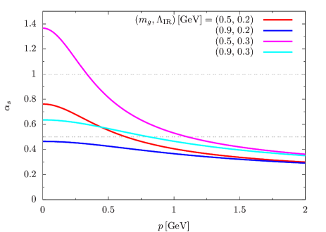
Figure 2: $\alpha_{s}$ in Eq.(28) as a function of (Euclidean) momentum $p\equiv\sqrt{Q^{2}}$ for several combinations of $m_{g}$ and $\Lambda_{\rm IR}$.

We use the OGE for the momentum transfer of $\lesssim 1$ GeV and hence have to specify how $\alpha_{s}$ behaves in the non-perturbative domain. How to define $\alpha_{s}$ is a highly nontrivial issue in its own (for a comprehensive summary, see Ref. Deur et al. (2016)). Our reference is the IR freezing picture for the running coupling constant Deur et al. (2016)

$$\alpha_{s}(Q^{2})=\frac{\,4\pi\,}{\,\beta_{0}\ln\frac{\,Q^{2}+m_{g}^{2}\,}{\,\Lambda_{\rm IR}^{2}\,}}\,,$$ (28)

where $\beta_{0}=(11N_{\rm c}-2N_{\rm f})/3$ with $N_{\rm c}$ and $N_{\rm f}$ being the number of colors and flavors, $Q^{2}$ a squared momentum transfer in the euclidean signature, $m_{g}$ a parameter of $\sim 0.5$-0.9 GeV, and $\Lambda_{\rm IR}\simeq 0.2$-0.3 GeV. The behaviors $\alpha_{s}$ are shown in Fig.2 where substantial dependence on $m_{g}$ and $\Lambda_{\rm IR}$ can be seen at $p\lesssim 1$ GeV. The inclusion of $m_{g}$ is motivated by the observation that gluonic fluctuations at long wavelength cannot grow arbitrarily in amplitudes and hence temper the RG evolution toward the IR limit, removing the perturbative Landau pole. The IR finite gluonic fluctuations are either due to the confining effects or the gluon saturation due to the self-coupling Gribov (1978). Models of massive gluons also lead to similar descriptions Curci and Ferrari (1976); Mandula and Ogilvie (1987); Reinosa et al. (2017, 2014); Suenaga and Kojo (2019); Song et al. (2019); Kojo and Suenaga (2021).

For the choice of $Q^{2}$, its typical magnitude is correlated with the typical momenta of quarks in a given problem, so we suppose $Q^{2}\sim\bar{{\bm{P}}^{2}}$ or $\bar{E}^{2}$. But in practice we use Eq.(28) as a mere qualitative guide, treating $\alpha_{s}$ as one of fitting parameters for mesons in a given channel, see Tables in Sec.IV. Then we examine a general tendency of $\alpha_{s}$ posteriori. It turns out that $\alpha_{s}$ is $\sim 0.7$-$0.8$ for light and strange quarks, and $\sim 0.4$ for charmed quarks, reasonably consistent with the behaviors shown in Fig.2.

III.3 Relativistic vertices

Computing the quark vertices coupled to gluons, we encounter the following types of terms

$$\sim\frac{\,k_{i}\,}{\,E_{1}({\bm{P}}+{\bm{k}}/2)\,}U({\bm{k}})\frac{\,k_{j}\,}{\,E_{2}({\bm{P}}-{\bm{k}}/2)\,}\,,$$ (29)

where the factor $\sim{\bm{k}}/E$ comes from the velocity factors at vertices. In our framework $E_{1,2}$ are replaced with the average $\bar{E}_{1,2}$. This simplification would leave artifacts as discussed below.

Neglecting the ${\bm{k}}$-dependence in the denominators, we obtain the factors $\sim k_{i}k_{j}/\bar{E}_{1}\bar{E}_{2}$. Such high powers in ${\bm{k}}$ combined with $U({\bm{k}})$ often result in singular potentials. For instance, with $i=j$ and $U({\bm{k}})=1/{\bm{k}}^{2}$, we have

$$\sim\frac{\,{\bm{k}}^{2}\,}{\,\bar{E}_{1}\bar{E}_{2}\,}\frac{\,1\,}{\,{\bm{k}}^{2}\,}~{}\rightarrow~{}\frac{\,1\,}{\,\bar{E}_{1}\bar{E}_{2}\,}\delta({\bm{r}})\,,$$ (30)

after taking the Fourier transform. This singular behavior is not problematic as far as we evaluate it in perturbation theories, but it would become problematic in unperturbed treatments. The singular behavior is just an artifact of abusing the replacement $|{\bm{k}}|/E\rightarrow|{\bm{k}}|/\bar{E}$ at large momenta; instead the correct behavior is $|{\bm{k}}|/E\rightarrow 1$ in large ${\bm{k}}$ limit and becomes harmless.

Taking the above considerations into account, we write the spinor matrices as

$$\bar{u}_{i}({\bm{p}})u_{i}({\bf q}) \rightarrow \frac{\,m_{i}\,}{\,\bar{E}_{i}\,}-\frac{\,(\mathrm{i}{\bm{k}})^{2}{\mathcal{K}}_{i}+4{\bm{\sigma}}_{i}\cdot(\mathrm{i}{\bm{k}}\times{\bm{P}}){\mathcal{L}}_{i}\,}{\,8\bar{E}_{i}\zeta_{i}\,}\,,$$

$$\bar{u}_{i}({\bm{p}})\gamma_{0}u_{i}({\bf q}) \rightarrow 1+\frac{\,(\mathrm{i}{\bm{k}})^{2}{\mathcal{K}}_{i}+4{\bm{\sigma}}_{i}\cdot(\mathrm{i}{\bm{k}}\times{\bm{P}}){\mathcal{L}}_{i}\,}{\,8\bar{E}_{i}\zeta_{i}\,}\,,$$

$$\bar{u}_{i}({\bm{p}}){\bm{\gamma}}u_{i}({\bf q}) \rightarrow \frac{\,2{\bm{P}}-(\mathrm{i}{\bm{k}}\times{\bm{\sigma}}_{i}){\mathcal{J}}_{i}\,}{\,2\bar{E}_{i}\,}\,.$$ (31)

where ${\mathcal{K}}_{i},{\mathcal{L}}_{i}$ and ${\mathcal{J}}_{i}$ ($i=1,2$) are form factors as functions of ${\bm{k}}$ to cutoff the UV singularity associated with large $|{\bm{k}}|$. If we set ${\mathcal{K}}_{i}={\mathcal{L}}_{i}={\mathcal{J}}_{i}=1$ we recover expressions without cutoff effects. In practice we assume the Gaussian factors, ${\mathcal{K}}_{i},{\mathcal{L}}_{i},{\mathcal{J}}_{i}\sim\mathrm{e}^{-{\rm const.}\times{\bm{k}}^{2}/\bar{E}_{i}^{2}}$, with which we get the expression similar to nonrelativistic expression at low ${\bm{k}}$. We distinguish the coefficients ${\mathcal{K}}_{i},{\mathcal{L}}_{i},{\mathcal{J}}_{i}$ as they characterize different physics.

We proceed with this approximation and take the Fourier transform to get the coordinate space expression. But we further simplify the expression while keeping the above qualitative features. The steps are detailed in Appendix.A. In short, we include the form factors for each potential and take the Fourier transform. For instance, terms with form factors ${\mathcal{K}}_{1}$ and ${\mathcal{K}}_{2}$ are converted into

$$\frac{\,(\mathrm{i}k_{i})(\mathrm{i}k_{j})\,}{\,f(E_{1},E_{2})\,}{\mathcal{K}}_{1}{\mathcal{K}}_{2}U({\bm{k}}) ~{}\rightarrow~{} \frac{\,\partial_{i}\partial_{j}\,}{\,f(\bar{E}_{1},\bar{E}_{2})\,}U_{\rm reg}^{{\mathcal{K}}_{1}{\mathcal{K}}_{2}}(r)\,,$$ (32)

where $f(E_{1},E_{2})$ is a general function of $E_{1,2}$ appearing in the denominator, and $U_{\rm reg}^{{\mathcal{K}}_{1}{\mathcal{K}}_{2}}$, with the upperscripts specifying the types of form factors, represents the short distance contributions,

$$U_{\rm reg}^{{\mathcal{K}}_{1}{\mathcal{K}}_{2}}=\mathrm{e}^{-\beta_{{\mathcal{K}}_{1}{\mathcal{K}}_{2}}^{2}r^{2}}\times U^{{\mathcal{K}}_{1}{\mathcal{K}}_{2}}_{\rm sh}\,,$$ (33)

with the strength averaged over distance $\sim\beta^{-1}$,

$$U_{\rm sh}^{{\mathcal{K}}_{1}{\mathcal{K}}_{2}}=\int_{0}^{\infty}\!\mathrm{d}\xi\,\xi^{2}w_{{\mathcal{K}}_{1}{\mathcal{K}}_{2}}(\xi)U^{{\mathcal{K}}_{1}{\mathcal{K}}_{2}}(\xi)\,,~{}~{}$$

$$w_{{\mathcal{K}}_{1}{\mathcal{K}}_{2}}(\xi)=\frac{\,4\beta_{{\mathcal{K}}_{1}{\mathcal{K}}_{2}}^{3}\,}{\,\sqrt{\pi}\,}\,\mathrm{e}^{-\beta_{{\mathcal{K}}_{1}{\mathcal{K}}_{2}}^{2}\xi^{2}}\,.$$ (34)

The parameter $\beta\sim\bar{E}$ is related to our form factors and hence depend on the types of potentials. In general, we write, for $s=\mathcal{K}_{i},\mathcal{L}_{i},\mathcal{K}_{1}\mathcal{K}_{2},\mathcal{J}_{1}\mathcal{J}_{2}$,

$$U_{\rm reg}^{s}=\mathrm{e}^{-\beta_{s}^{2}r^{2}}\times U^{s}_{\rm sh}\,,~{}~{}~{}$$

$$U_{\rm sh}^{s}=\int_{0}^{\infty}\!\mathrm{d}\xi\,\xi^{2}w_{s}(\xi)U^{s}(\xi)\,,~{}~{}w_{s}(\xi)=\frac{\,4\beta_{s}^{3}\,}{\,\sqrt{\pi}\,}\,\mathrm{e}^{-\beta_{s}^{2}\xi^{2}}\,.$$ (35)

Here $\beta_{s}$’s are parametrized as

$$\beta_{\mathcal{K}_{i}}=C_{\mathcal{K}_{i}}\bar{E}_{i}\,,~{}~{}~{}~{}\beta_{\mathcal{L}_{i}}=C_{\mathcal{L}_{i}}\bar{E}_{i}\,,$$

$$\beta_{\mathcal{K}_{1}\mathcal{K}_{2}}=C_{\mathcal{K}_{1}\mathcal{K}_{2}}\bar{E}_{\rm red}\,,~{}~{}~{}~{}\beta_{\mathcal{J}_{1}\mathcal{J}_{2}}=C_{\mathcal{J}_{1}\mathcal{J}_{2}}\bar{E}_{\rm red}\,,$$ (36)

where $C$’s are treated as constants of $O(1)$, and

$$\bar{E}_{\rm red}^{-2}\equiv\bar{E}_{1}^{-2}+\bar{E}_{2}^{-2}\,.$$ (37)

Below we often omit the subscripts ${\mathcal{K}}_{i},{\mathcal{L}}_{i}$, and ${\mathcal{J}}_{i}$ to avoid busy notations.

In this paper we work only up to the second order of ${\bm{k}}^{2}$ to which each vertex contribute to one power of $k$. We use the following notations for our replacement procedures,

$$(\mathrm{i}{\bm{k}})_{i}(\mathrm{i}{\bm{k}})_{j}\tilde{U}~{} \rightarrow ~{}\delta_{ij}\bar{U}_{2}(r)/3+Q_{ij}\bar{U}_{2T}(r)/3\,,$$

$$(\mathrm{i}{\bm{k}}\times{\bm{P}})\tilde{U}~{} \rightarrow ~{}{\bm{L}}\bar{U}_{1L}(r)\,,$$

$$(\mathrm{i}{\bm{k}}\times{\bm{P}})_{i}(\mathrm{i}{\bm{k}}\times{\bm{P}})_{j}\tilde{U}~{} \rightarrow ~{}\mathcal{P}_{ij}\bar{U}_{2\mathcal{P}}(r)+L_{i}L_{j}\bar{U}_{2L^{2}}(r)\,,$$

where we have defined

$$Q_{ij}=\delta_{ij}-\frac{\,3x_{i}x_{j}\,}{\,r^{2}\,}\,,~{}~{}~{}\mathcal{P}_{ij}=\delta_{ij}{\bm{P}}^{2}-P_{i}P_{j}\,.$$ (39)

The subscript of $\bar{U}$ indicates the powers of ${\bm{k}}$. Explicitly, each potential is computed from $U_{\rm inter}$ as

$$\bar{U}_{2}={\bm{\nabla}}^{2}U_{\rm reg}\,,~{}~{}~{}~{}\bar{U}_{2T}=-\bigg{(}\frac{\,\mathrm{d}^{2}\,}{\,\mathrm{d}r^{2}\,}-\frac{1}{\,r\,}\frac{\,\mathrm{d}\,}{\,\mathrm{d}r\,}\bigg{)}U_{\rm reg}\,,$$

$$~{}~{}~{}~{}~{}~{}~{}~{}~{}\bar{U}_{1L}(r)=\bar{U}_{2\mathcal{P}}(r)=\frac{1}{\,r\,}\frac{\,\mathrm{d}U_{\rm reg}\,}{\,\mathrm{d}r\,}\,,$$

$$~{}~{}~{}~{}~{}~{}~{}\bar{U}_{2L^{2}}(r)=\frac{1}{\,r^{2}\,}\bigg{(}\frac{\,\mathrm{d}^{2}\,}{\,\mathrm{d}r^{2}\,}-\frac{1}{\,r\,}\frac{\,\mathrm{d}\,}{\,\mathrm{d}r\,}\bigg{)}U_{\rm reg}\,.$$ (40)

Some useful formulae are summarized in Appendix.B.

III.4 The full expressions of potentials

Convoluting the quark vertices and the potentials $U$’s, we obtain

$$\bar{V} = \bar{V}_{C}^{(0)}+\bar{V}_{C}^{(2)}+\bar{V}_{ss}({\bm{\sigma}}_{1}\cdot{\bm{\sigma}}_{2})+\bar{V}_{L^{2}}{\bm{L}}^{2}$$ (41)

$$+\sum_{i=1,2}\bar{V}^{(i)}_{sL}({\bm{\sigma}}_{i}\cdot{\bm{L}})+\bar{V}_{(sL)^{2}}({\bm{\sigma}}_{1}\cdot{\bm{L}})({\bm{\sigma}}_{2}\cdot{\bm{L}})$$

$$+\,\bar{V}_{T}\big{(}{\bm{\sigma}_{1}}\cdot{\bm{Q}}\cdot{\bm{\sigma}_{2}}\big{)}\,.$$

The first term is the central potential without spatial derivatives

$$\bar{V}_{C}^{(0)}=\bigg{(}1+\frac{\,\bar{{\bm{P}}}^{2}\,}{\,\bar{E}_{1}\bar{E}_{2}\,}\bigg{)}\bigg{(}U^{V}_{\rm conf}+U_{\rm OGE}^{V}\bigg{)}+\frac{\,m_{1}m_{2}\,}{\,\bar{E}_{1}\bar{E}_{2}\,}U^{S}_{\rm conf}\,.$$

(42)

As we will see, this term plays the dominant roles in determining the overall spectra. All the other terms contain the spatial derivatives of the potentials. The central potential with spatial derivatives is $(\zeta_{i}\equiv\bar{E}_{i}+m_{i}$)

$$\bar{V}_{C}^{(2)} = \frac{\,1\,}{\,8\,}\bigg{(}\frac{\,\bar{U}^{{\mathcal{K}}_{1}}_{2}\,}{\,\bar{E}_{1}\zeta_{1}\,}+\frac{\,\bar{U}^{{\mathcal{K}}_{2}}_{2}\,}{\,\bar{E}_{2}\zeta_{2}\,}\bigg{)}\bigg{|}_{U=U_{\rm OGE}^{V}+U_{\rm conf}^{V}}$$ (43)

$$-\frac{\,1\,}{\,8\,}\bigg{(}\frac{\,\bar{U}^{{\mathcal{K}}_{1}}_{2}\,}{\,\bar{E}_{1}\zeta_{1}\,}\frac{\,m_{2}\,}{\,\bar{E}_{2}\,}+\frac{\,\bar{U}^{{\mathcal{K}}_{2}}_{2}\,}{\,\bar{E}_{2}\zeta_{2}\,}\frac{\,m_{1}\,}{\,\bar{E}_{1}\,}\bigg{)}\bigg{|}_{U=U_{\rm conf}^{S}}\,.$$

The spin-spin interaction is given by

$$\bar{V}_{ss} = \frac{\,1\,}{\,6\bar{E}_{1}\bar{E}_{2}\,}\bigg{(}\bar{U}_{2}^{{\mathcal{J}}_{1}{\mathcal{J}}_{2}}+\frac{\,{\bm{P}}^{2}\,}{\,\zeta_{1}\zeta_{2}\,}\bar{U}_{2\mathcal{P}}^{{\mathcal{J}}_{1}{\mathcal{J}}_{2}}\bigg{)}\bigg{|}_{U=U_{\rm OGE}^{V}+U_{\rm conf}^{V}}$$ (44)

$$+\frac{\,\bar{{\bm{P}}}^{2}\,}{\,6\bar{E}_{1}\bar{E}_{2}\zeta_{1}\zeta_{2}\,}\bar{U}_{2\mathcal{P}}^{{\mathcal{J}}_{1}{\mathcal{J}}_{2}}\bigg{|}_{U=U_{\rm conf}^{S}}\,.$$

The potential giving additional centrifugal forces

$$\bar{V}_{{\bm{L}^{2}}}=\frac{\,1\,}{\,2\bar{E}_{1}\bar{E}_{2}\,}\bar{U}_{1L}^{{\mathcal{J}}_{1}{\mathcal{J}}_{2}}\big{|}_{U=U_{\rm OGE}^{V}}\,,$$ (45)

which arise only from the $k_{i}k_{j}/{\bm{k}}^{2}$ term in the one gluon exchange. The potential for the spin-orbit coupling is given by

$$\bar{V}^{(i=1)}_{sL} = \bigg{(}\frac{1}{\bar{E}_{1}\zeta_{1}}+\frac{1}{\,\bar{E}_{1}\bar{E}_{2}\,}\bigg{)}\frac{\,\bar{U}^{{\mathcal{L}}_{1}}_{1L}}{2}\bigg{|}_{U=U_{\rm OGE}^{V}+U_{\rm conf}^{V}}$$ (46)

$$-~{}\frac{1}{\,\bar{E}_{1}\zeta_{1}\,}\frac{m_{2}}{\,\bar{E}_{2}\,}\frac{\,\bar{U}^{{\mathcal{L}}_{1}}_{1L}}{2}\bigg{|}_{U=U_{\rm conf}^{S}}\,.$$

The $\bar{V}^{(i=2)}_{sL}$ is obtained by swapping 1 and 2.

The potential for the square of the spin-orbit coupling operators is

$$\bar{V}_{(sL)^{2}}=\frac{\,\bar{U}_{2L^{2}}^{{\mathcal{J}}_{1}{\mathcal{J}}_{2}}\,}{\,4\bar{E}_{1}\bar{E}_{2}\zeta_{1}\zeta_{2}\,}\bigg{|}_{U=U_{\rm OGE}^{V}+U_{\rm conf}^{V}+U_{\rm conf}^{S}}\,.$$ (47)

Finally, the tensor potential is

$$\bar{V}_{T}=-\frac{\,\bar{U}_{2T}^{{\mathcal{J}}_{1}{\mathcal{J}}_{2}}\,}{\,12\bar{E}_{1}\bar{E}_{2}\,}\bigg{|}_{U=U_{\rm OGE}^{V}+U_{\rm conf}^{V}}\,.$$ (48)

The tensor term is regarded as small and treated in perturbation theories.

III.5 Bases and matrix elements

The potential Eq.(41) contains operators of spin, orbital angular momenta and tensor couplings. The operators ${\bm{J}}^{2}$ and $J_{z}$, made of total angular momentum ${\bm{J}}={\bm{L}}+{\bm{S}}$, commute with all operators in the potential. Meanwhile, the ${\bm{L}}^{2}$ operator is in general not conserved due to the tensor forces that mix, e.g., $L=0$ and $L=2$ states. Also the total spin is not conserved for mesons including unequal quark masses. Our strategy is to use bases with definite $(J,J_{z},L,S)$ and treat the terms that violate $L$ and $S$ conservations as perturbations. In this paper we omit such perturbative corrections when we perform fitting to the meson spectra, but we summarize some expressions needed to evaluate such matrix elements for the future studies.

III.5.1 Equal mass

The total spin $S$ operator in general does not commute with the $\sum_{i=1,2}\bar{V}^{(i)}_{sL}({\bm{\sigma}}_{i}\cdot{\bm{L}})$ operator. The exception is the case with equal mass $m_{1}=m_{2}$ for which the operator can be expressed as

$$\sum_{i=1,2}\bar{V}^{(i)}_{sL}({\bm{\sigma}}_{i}\cdot{\bm{L}})=\bar{V}_{sL}({\bm{\sigma}}\cdot{\bm{L}})$$ (49)

with ${\bm{\sigma}}={\bm{\sigma}}_{1}+{\bm{\sigma}}_{2}$ and $\bar{V}^{(1)}_{sL}=\bar{V}^{(2)}_{sL}=\bar{V}_{sL}$. Hence, we use the bases ($C^{J,J_{z}}_{L,L_{z};S,S_{z}}$: Clebsch-Gordan coefficients),

$$|J,J_{z}\rangle_{L,S}=\sum_{L_{z},S_{z}}C^{J,J_{z}}_{L,L_{z};S,S_{z}}|L,L_{z}\rangle\otimes|S,S_{z}\rangle\,.$$ (50)

For mesonic systems, the total spin is $S=0$ or $1$. With these bases, the matrix elements of operators (which are diagonal for $(J,J_{z},L,S)$) are evaluated. The spin-spin operator takes the usual form,

$$\langle{\bm{\sigma}}_{1}\cdot{\bm{\sigma}}_{2}\rangle^{J,J_{z}}_{L,S}=2S(S+1)-3\,.$$ (51)

The spin-orbit operator is evaluated as

$$\langle{\bm{L}}\cdot{\bm{\sigma}}\rangle^{J,J_{z}}_{L,S}=2C_{LS}^{J}\,,$$ (52)

with

$$C_{LS}^{J}\equiv\frac{\,J(J+1)-L(L+1)-S(S+1)\,}{2}\,.$$ (53)

Also, one can compute

$$\langle({\bm{L}}\cdot{\bm{\sigma}}_{1})({\bm{L}}\cdot{\bm{\sigma}}_{2})\rangle^{J,J_{z}}_{L,S}=D_{LS}^{J}\,,$$ (54)

with

$$D_{LS}^{J}\equiv 2\big{(}C_{LS}^{J}\big{)}^{2}+C_{LS}^{J}-L(L+1)\,.$$ (55)

III.5.2 Unequal mass

For unequal masses, $S$ is not a good quantum number. The bases must be a superposition of $S=0$ and $1$ states.

$$|J,J_{z}\rangle_{L}\equiv\alpha|J,J_{z}\rangle_{L,S=1}+\beta|J,J_{z}\rangle_{L,S=0}\,.$$ (56)

For a given $L$, the possible $J$’s are $L+1,L$, and $|L-1|$. The cases $J=L+1$ and $|L-1|$ are possible only when $S=1$, so $\alpha=1$ and $\beta=0$. The matrix elements for ${\bm{L}}\cdot{\bm{\sigma}}_{1,2}$ are

$$\langle L+1,J_{z}|({\bm{L}}\cdot{\bm{\sigma}}_{1,2})|L+1,J_{z}\rangle_{L,S=1}=L\,,$$

$$\langle L-1,J_{z}|({\bm{L}}\cdot{\bm{\sigma}}_{1,2})|L-1,J_{z}\rangle_{L,S=1}=-(L+1)\,,$$ (57)

where the expression for $L-1$ is valid for $L\geq 1$.

For $J=L$, we determine $\alpha$ and $\beta$ for a given $(J,L)$ by diagonalizing the hamiltonian with the following mixing terms (the upper are $(S,S^{\prime})=(1,1)$ and $(1,0)$ components, the lower $(0,1)$ and $(0,0)$ components),

$$\bigg{\langle}\sum_{i=1,2}\bar{V}^{(i)}_{sL}({\bm{\sigma}}_{i}\cdot{\bm{L}})\bigg{\rangle}^{J=L,L}_{S,S^{\prime}}$$

$$=\left[\begin{matrix}-\bar{V}^{(1+2)}_{sL}&-\sqrt{L(L+1)\,}\,\bar{V}^{(1-2)}_{sL}\,\\ \,-\sqrt{L(L+1)\,}\,\bar{V}^{(1-2)}_{sL}\,&0\end{matrix}\right]^{J=L,L}$$

where $\bar{V}^{(1\pm 2)}_{sL}=\bar{V}^{(1)}_{sL}\pm\bar{V}^{(2)}_{sL}$. Here the $L=0$ case is exceptional because of complete decoupling of $S=1$ and $0$ states.

Table 1: Meson spectra for the $L=0$ states from light to charm quark sectors. The experimental meson mass $M_{\rm exp}$, our result $M_{\rm th}$, the average momenta which satisfy the consistency, $\bar{{\bm{P}}}^{2}\simeq\langle{\bm{P}}^{2}\rangle$, are given in GeV units, while the root-mean-square radii $\sqrt{\langle{\bm{r}}^{2}\rangle\,}$ are given in fm unit. Our choices for $f_{S}$ and $\alpha_{s}$ are also displayed. (* for unestablished states.)

	$n_{r}$${}^{2S+1}L_{J}$	$M_{\rm exp}$	$M_{\rm cal}$	$\bar{{\bm{P}}}^{2}$	$\sqrt{\langle{\bm{r}}^{2}\rangle}$	$f_{S}$	$\alpha_{s}$
$\pi$	$1^{1}S_{0}$	0.14	0.16	0.47	0.50	0.70	0.80
	$2^{1}S_{0}$	1.30	1.28	0.43	0.98
	$3^{1}S_{0}$	1.81	1.82	0.55	1.38
	$4^{1}S_{0}$	2.07**	2.22	0.67	1.66
$\rho$	$1^{3}S_{1}$	0.78	0.76	0.21	0.66	0.74	0.80
	$2^{3}S_{1}$	1.47	1.44	0.35	1.17
	$3^{3}S_{1}$	1.91*	1.87	0.48	1.55
	$4^{1}S_{1}$	2.27**	2.22	0.61	1.83
$K$	$1^{1}S_{0}$	0.49	0.49	0.42	0.49	0.72	0.77
	$2^{1}S_{0}$	1.46*	1.46	0.45	0.98
$K^{*}$	$1^{3}S_{1}$	0.89	0.91	0.24	0.63	0.75	0.77
	$2^{3}S_{1}$	1.41	1.54	0.39	1.10
$\eta_{s}$	$1^{1}S_{0}$	0.74	0.71	0.45	0.47	0.73	0.75
	$2^{1}S_{0}$	1.48	1.66	0.46	0.99
	$3^{1}S_{0}$	2.10	2.12	0.59	1.37
$\phi$	$1^{3}S_{1}$	1.02	1.03	0.30	0.57	0.76	0.75
	$2^{3}S_{1}$	1.68	1.71	0.43	1.06
	$3^{1}S_{1}$	2.18	2.12	0.56	1.44
$D$	$1^{1}S_{0}$	1.87	1.87	0.39	0.50	0.73	0.58
	$2^{1}S_{0}$	—	2.50	0.47	0.99
$D^{*}$	$1^{3}S_{1}$	2.01	2.00	0.29	0.56	0.76	0.58
	$2^{3}S_{1}$	2.64*	2.53	0.44	1.04
$D_{s}$	$1^{1}S_{0}$	1.97	1.96	0.52	0.44	0.73	0.57
	$2^{1}S_{0}$	—	2.66	0.56	0.91
$D_{s}^{*}$	$1^{3}S_{1}$	2.11	2.12	0.37	0.50	0.76	0.57
	$2^{3}S_{1}$	2.73	2.70	0.51	0.96
$\eta_{c}$	$1^{1}S_{0}$	2.98	2.98	0.79	0.35	0.73	0.42
	$2^{1}S_{0}$	3.64	3.62	0.81	0.78
$J/\psi$	$1^{3}S_{1}$	3.10	3.09	0.56	0.40	0.77	0.42
$\psi$	$2^{3}S_{1}$	3.69	3.66	0.71	0.82

Table 2: The average quark energy vs composition of the potential energies for mesons with equal quark masses, $m_{1}=m_{2}$. The unit is GeV. We use the following conventions for the evaluation of potential energies: $\langle O_{C}^{(0,2)}\rangle=\langle\bar{V}_{C}^{(0,2)}\rangle$ and $\langle O_{ss}\rangle=\langle\bar{V}_{ss}({\bm{\sigma}}_{1}\cdot{\bm{\sigma}}_{2})\rangle$.

	$M_{\rm cal}$	$\bar{{\bm{P}}}^{2}$	$\bar{E}_{1,2}$	$\langle O_{C}^{(0)}\rangle$	$\langle O_{C}^{(2)}\rangle$	$\langle O_{ss}\rangle$
$\pi$	0.16	0.47	$0.75$	$-1.01$	$0.10$	$-0.34$
	1.28	0.43	$0.72$	$-0.07$	$0.03$	$-0.12$
$\rho$	0.76	0.21	$0.54$	$-0.43$	$0.05$	$0.05$
	1.44	0.35	$0.66$	$0.06$	$0.04$	$0.04$
$\eta_{s}$	0.71	0.45	$0.83$	$-0.82$	$0.07$	$-0.17$
	1.66	0.46	$0.83$	$0.03$	$0.03$	$-0.05$
$\phi$	1.03	0.30	$0.73$	$-0.49$	$0.05$	$0.04$
	1.71	0.43	$0.82$	$0.05$	$0.03$	$0.02$
$\eta_{c}$	2.98	0.79	$1.70$	$-0.37$	$0.02$	$-0.07$
	3.62	0.81	$1.71$	$0.26$	$0.01$	$-0.04$
$J/\psi$	3.09	0.56	$1.63$	$-0.20$	$0.01$	$0.01$
$\psi$	3.66	0.71	$1.67$	$0.31$	$0.01$	$0.01$

IV Meson spectra

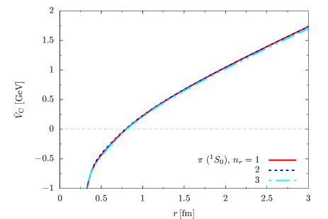
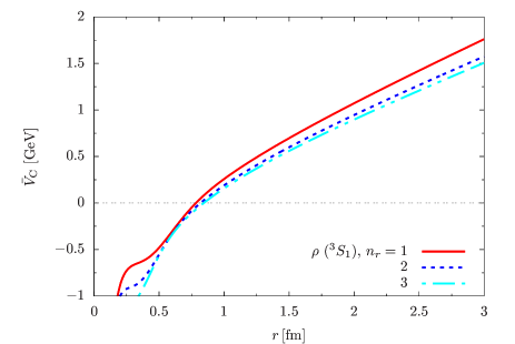
Figure 3: The potential $\bar{V}_{C}$ for $\pi\,(^{1}S_{0})$ (upper panel) and $\rho\,(^{3}S_{1})$ (lower panel) states with radial excitations up to $n_{r}=3$. The potential depends on the average momentum $\bar{{\bm{P}}}^{2}$ in a given meson. Small bumps in the $\rho$ channel originate from the spin-spin repulsions at short distance.

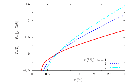
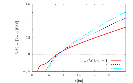
Figure 4: The effective potential $[\mathcal{V}_{M}]_{C}=I_{M}\bar{V}_{C}$ for $\pi\,(^{1}S_{0})$ (upper panel) and $\rho\,(^{3}S_{1})$ (lower panel) states with radial excitations up to $n_{r}=3$. The effective potential includes the relativistic kinematic factor $I_{M}$ in Eq.(2) which depend on the meson mass and $\bar{E}_{1,2}$. In the nonrelativistic limit for equal masses, the factor $I_{M}$ is a constant, $I_{M}=m_{1}=m_{2}$.

In this section we fit our model calculations to the experimental meson spectra. We focus on ordinary mesons which are regarded as $q\bar{q}$, omitting extraordinary mesons such as $\eta^{\prime}$, which is substantially affected by the topological fluctuations ’t Hooft (1976a, b); Witten (1979b), or scalar mesons, $\sigma,\kappa,f_{0}(980),a_{0}(980)$, which are often discussed as tetraquark candidates including intermediate states with the $q\bar{q}$ annihilations or mesonic molecule states Jaffe (1977); Isgur (1976); Pelaez (2016).

There are several states for which assignments of quantum numbers are not obvious. For mesons made of light and strange quarks, we follow the identification made by Ebert et al. where the list of mesons is summarized in Table I in Ref.Ebert et al. (2009). For light-heavy mesons, we refer to Table 1 in Ref.Ebert et al. (2010). If the assigned states are not well established in the particle data group (PDG) Zyla et al. (2020), we attach * to the experimental mass $M_{\rm exp}$. We attach ** for states in “further states” Section in the PDG.

As we have seen in the previous sections, our model contains many parameters which cannot be directly derived from our model. The list is

$$(m_{ud},\,m_{s},\,m_{c}),\,f_{S},\,\alpha_{s},\,C_{\mathcal{K}_{i}},\,C_{\mathcal{L}_{i}},\,C_{\mathcal{J}_{1}\mathcal{J}_{2}}\,.$$ (59)

Moreover these parameters may depend on dynamics and thus may change for a given meson. We try to keep these parameters common for different channels as much as possible. But we found it necessary to make some parameters non-universal. Below we examine when we need to compromise with non-universal treatments.

We take the constituent quark masses common for whole mesons,

$$(m_{ud},\,m_{s},\,m_{c})=(0.30,\,0.48,\,1.45)\,{\rm GeV}\,,$$ (60)

which are typical in constituent quark models. Some variations are possible and the effects can be largely absorbed by retuning the values of $\alpha_{s}$.

We found that the value of $f_{S}$ cannot be taken common for whole spectra and should vary from $\simeq 0.70$ to $\simeq 0.83$. Light flavor mesons favor smaller values. The trend $f_{s}>0.5$ means that the scalar confinement vertex is larger than the vector one. In this respect our confining part is closer to Godfrey et al. with $f_{S}=1$ than to Ebert et al. with $f_{S}=-1$.

The $\alpha_{s}$ values are sensitive to the flavors of mesons which are related to the quark energies. For our choice of the quark masses, $\alpha_{s}$ ranges from $\simeq 0.8$ for light quarks to $\simeq 0.3$ for charm quarks. For mesons with unequal quark masses $m_{f}\neq m_{f^{\prime}}$, we found that the following estimate works reasonably well for the effective coupling $\alpha_{s}^{ff^{\prime}}$,

$$\alpha_{s}^{ff^{\prime}}\simeq\sqrt{\alpha_{s}^{f}\alpha_{s}^{f^{\prime}}}\,,$$ (61)

where $\alpha_{s}^{f}$ is the value used for a meson made of $m_{1}=m_{2}=m_{f}$. The details depend on the channels, and we allow variation of $\lesssim 10$% in our fitting procedures.

For $C$’s appearing in the form factors, it should be $O(1)$ by construction. We found that $C_{\mathcal{J}_{1}\mathcal{J}_{2}}$ and $C_{\mathcal{L}_{i}}$, which appear in spin-spin forces and $LS$ respectively, need some arrangements. Meanwhile, the spectra are not very sensitive to $C_{\mathcal{K}_{i}}$ as far as we take the values close to $\simeq 1$. We choose

$$C_{\mathcal{L}_{i}}=0.5\,,~{}~{}~{}C_{\mathcal{K}_{i}}=1\,,~{}~{}~{}C_{\mathcal{J}_{1}\mathcal{J}_{2}}=1.0-1.5\,.$$ (62)

We found that the values of $C_{\mathcal{J}_{1}\mathcal{J}_{2}}$ should deviate from $1$ for mesons including light quarks, i.e., $ud$, $us$, and $ss$ mesons for good fits.

In our fitting procedures we omit tensor forces (which mix different $L$) and $({\bm{s}}_{1}-\bm{s}_{2})\cdot{\bm{L}}$ type LS forces (which mix $S=0$ and 1 states). While these terms make our fitting procedures more nonlinear and involved, we expect that their impacts are not very significant at the quality of fit we are aiming at in this paper.

IV.1 $L=0$ states

Figure 5: The $f_{S},\alpha_{s},C_{\mathcal{J}_{1}\mathcal{J}_{2}}$ dependence of the masses of $\pi,\rho,\eta_{s},\phi$ for the 0th (solid lines) and the 1st radial excitations (dashed lines). The superscript “base” refers to the baseline values which we chose for Table.1. Each parameter is varied up to $\pm 10$% from the baseline values.

The $L=0$ states depend on the central and spin-spin potentials,

$$\bar{V}_{L=0} = \bar{V}_{C}^{(0)}+\bar{V}_{C}^{(2)}+\bar{V}_{ss}({\bm{\sigma}}_{1}\cdot{\bm{\sigma}}_{2})\,.$$ (63)

In order to achieve good fits, we take $C_{\mathcal{J}_{1}\mathcal{J}_{2}}=1.5$ for the $ud$-mesons, $C_{\mathcal{J}_{1}\mathcal{J}_{2}}=1.3$ for the $us$-mesons, and for the others we set $C_{\mathcal{J}_{1}\mathcal{J}_{2}}=1$. The parameter $C_{\mathcal{L}_{i}}$ does not show up in the $L=0$ states and are left unfixed.

In Table.1 we display the experimental meson mass $M_{\rm exp}$, our result $M_{\rm th}$, the average momenta which satisfy the consistency, $\bar{{\bm{P}}}^{2}\simeq\langle{\bm{P}}^{2}\rangle$, and the root-mean-square radii $\sqrt{\langle{\bm{r}}^{2}\rangle\,}$. In Table.2 we show the composition of the potential energies for mesons with equal mass quarks, together with the average quark energy $\bar{E}_{1,2}$. The calculated masses fit the experimental ones very well from the light to charm quark sectors, although this is probably not very surprising because we have many parameters. What is important here is to examine the impact of each parameter and its trend.

Shown in Fig.3 are the potentials $\bar{V}_{C}$ which depend on meson masses and $\bar{{\bm{P}}}^{2}$. The cases for $\pi\,(^{1}S_{0})$ (upper panel) and $\rho\,(^{3}S_{1})$ (lower panel) states with radial excitations up to $n_{r}=3$ are displayed. Small bumps in the $\rho$ channel originate from the spin-spin repulsions at short distance. For our choice of $f_{S}\simeq 0.70$-0.75, it turns out that the potentials do not show large sensitivity to the values of $\bar{{\bm{P}}}^{2}$. In Fig.4, we show the potentials $[\bar{\mathcal{V}}_{M}]_{C}$ where the relativistic kinematic factors $I_{M}$’s in Eq.(2) are multiplied to $\bar{V}_{C}$. For equal quark masses $m_{1}=m_{2}$, the factor $I_{M}=(M+\bar{E}_{1}+\bar{E}_{2})/4$ depends on the meson mass and the quark energy. It becomes larger for a heavier meson, unlike the non-relativistic case where $I_{M}=m_{1,2}$ is a constant (see, Eq.(16)).

Given our fits, we found general trends: (i) To reproduce the masses of excited states, we had to tune $f_{S}$ for given channels. The trends we found are that $f_{S}$ should be taken smaller for the spin-singlet states than the triplet case, and $f_{S}$ gently grows toward the charm quark sector. (ii) For a given flavor combination, it turns out that we can fit the spectra using the common $\alpha_{s}$, although it is not necessary from the physics point of view. The value of $\alpha_{s}$ decreases toward the heavy quark sector, as it should. (iii) The momenta are in general sizable compared to the quark masses, even for the charm quark case. The resultant large average quark energies are largely cancelled with the Coulomb attraction energies $\bar{V}_{C}^{(0)}$. Due to this structure, the choice of $\alpha_{s}$ is crucial. (iv) The second order central potential $\bar{V}_{C}^{(2)}$ is much smaller than the leading order. This corrections contain the uncertainties associated with the choice of $C_{\mathcal{K}_{i}}$, but the details are not very important and thus we simply take $C_{\mathcal{K}_{i}}=1$. (v) The spin-spin potential $\bar{V}_{ss}$ is sizable for the $n_{r}=0$, spin-singlet states as in conventional non-relativistic models. Meanwhile, the spin-spin repulsion in the triplet channel is not as large as in the non-relativistic models.

While the above qualitative trends are commonly found for various parameter sets, the quantitative details of the mass spectra are rather sensitive to the parameters. To examine the importance of fine-tuning for parameters $f_{S},\alpha_{s}$, and $C_{\mathcal{J}_{1}\mathcal{J}_{2}}$, we perform linear analyses in which we change one of these parameters by $\sim 10$% while fix all the other parameters. In Fig.5 we show the results for $\pi,\rho,\eta_{s},\phi$ including the 0th and 1st radial excitations. During this analysis we always arrange $\bar{{\bm{P}}}^{2}\simeq\langle{\bm{P}}^{2}\rangle$ in good accuracy within our grids, $\Delta\bar{{\bm{P}}}^{2}=0.01\,{\rm GeV}^{2}$.

The correlations among these three parameters and the spectra are relatively simple to understand. The 10% variation of $f_{S}$ introduces the marginal changes in the 0th radial excitations while induces the mass changes of $\sim 200$ MeV for the 1st radial excitations. Mesons with heavier flavors have more compact structures and thus are less affected by the details of confining potentials.

The 10% variation of $\alpha_{s}$ has very large effects on the spin-singlet states. For $\pi$ and $\eta_{s}$, the mass variation is $\sim 300$-$400$ MeV. For the spin triplet states, $\rho$ and $\phi$, the impacts are smaller but still are $\sim 100$-$200$ MeV. The difference between the singlet and triplet states is the spin-spin correlations which make mesons more compact for the spin-singlet states; $\pi$ and $\eta_{s}$ have more chances to reduce the masses by forming the compact wavefunctions. For heavier flavors or higher radial excitations, the effects of $\alpha_{s}$ become weaker.

The 10% variation of $C_{\mathcal{J}_{1}\mathcal{J}_{2}}$ has large impacts on the spin singlet states, while the spin triplet states are not much affected.

After observing these correlations among the parameters and the spectra, our fitting strategy has been fixed as follows. We first explored the reasonable range of $\alpha_{s}$ to fit the spin triplet states in the 0th radial excitations which are relatively insensitive to $f_{S}$ and $C_{\mathcal{J}_{1}\mathcal{J}_{2}}$. Then, we tuned $C_{\mathcal{J}_{1}\mathcal{J}_{2}}$ to fit the spin singlet states. In the third step we chose $f_{S}$ to fit the radial excitations. The rest requires the fine tuning of all these parameters slightly. The last step is to examine whether the chosen parameters show qualitatively acceptable trends. We believe that the parameters shown in Table.1 are reasonable. For instance, the range of $\alpha_{s}$ used in the fit is consistent with Eq.(28).

IV.2 $L\geq 1$ states

Table 3: The meson spectra for the $L=1$ states with the conventions same as Table.1. From top to bottom, $ud$, $us$, $ss$, $uc$, $us$, and $cc$ mesons. The scalar mesons ${}^{3}P_{0}$ are omitted.

	$n_{r}$${}^{2S+1}L_{J}$	$M_{\rm exp}$	$M_{\rm cal}$	$\bar{{\bm{P}}}^{2}$	$\sqrt{\langle{\bm{r}}^{2}\rangle}$	$f_{S}$	$\alpha_{s}$
$b_{1}$	$1^{1}P_{1}$	1.23	1.27	0.25	0.99	0.77	0.80
	$2^{1}P_{1}$	—	1.70	0.37	1.46
	$3^{1}P_{1}$	1.96**	2.06	0.48	1.82
$a_{1}$	$1^{3}P_{1}$	1.23	1.19	0.28	0.94
	$2^{3}P_{1}$	1.65	1.68	0.41	1.44
	$3^{3}P_{1}$	2.10**	2.03	0.48	1.81
$a_{2}$	$1^{3}P_{2}$	1.32	1.33	0.23	1.03
	$2^{3}P_{2}$	1.73	1.74	0.36	1.47
	$3^{3}P_{2}$	2.05**	2.07	0.47	1.84
$K_{1}$	$1P_{1}$	1.40	1.40	0.28	0.95	0.80	0.79
	$2P_{1}$	—	1.80	0.44	1.35
$K_{1}$	$1P_{1}$	1.27	1.31	0.30	0.90
	$2P_{1}$	1.65*	1.77	0.42	1.35
$K_{2}^{*}$	$1^{3}P_{2}$	1.42	1.47	0.25	1.01
	$2^{3}P_{2}$	1.98*	1.85	0.41	1.39
$h_{1}$	$1^{1}P_{1}$	1.39	1.55	0.33	0.80	0.80	0.78
	$2^{1}P_{1}$	1.60*	1.70	0.42	1.37
$f_{1}$	$1^{3}P_{1}$	1.43	1.44	0.42	0.80
	$2^{3}P_{1}$	1.97*	1.88	0.54	1.24
$f^{\prime}_{2}$	$1^{3}P_{2}$	1.53	1.62	0.28	0.94
	$2^{3}P_{2}$	2.01	2.03	0.42	1.36
$D_{1}$	$1P_{1}$	2.42	2.40	0.34	0.86	0.80	0.55
	$2P_{1}$	—	2.72	0.49	1.27
$D_{1}$	$1P_{1}$	2.43	2.36	0.38	0.81
	$2P_{1}$	—	2.72	0.51	1.24
$D_{2}^{*}$	$1^{3}P_{2}$	2.46	2.44	0.30	0.90
	$2^{3}P_{2}$	—	2.79	0.45	1.31
$D_{s1}$	$1P_{1}$	2.54	2.57	0.41	0.78	0.80	0.55
	$2P_{1}$	—	2.95	0.57	1.18
$D_{s1}$	$1P_{1}$	2.46	2.52	0.46	0.75
	$2P_{1}$	—	2.91	0.60	1.15
$D_{s2}$	$1^{3}P_{2}$	2.57	2.60	0.37	0.81
	$2^{3}P_{2}$	—	2.98	0.53	1.21
$h_{c}$	$1^{1}P_{1}$	3.53	3.53	0.59	0.65	0.80	0.40
	$2^{1}P_{1}$	—	3.92	0.80	0.99
$\chi_{c1}$	$1^{3}P_{1}$	3.51	3.51	0.63	0.63
	$2^{3}P_{1}$	3.87	3.90	0.83	0.98
$\chi_{c2}$	$1^{3}P_{2}$	3.56	3.54	0.58	0.65
	$2^{3}P_{2}$	3.93	3.93	0.77	1.00

Table 4: The meson spectra for the $L=2$ states with the conventions same as Table.1. From top to bottom, $ud$, $us$, $ss$ mesons. Most of mesons with charm quarks are not experimentally confirmed, so we omit them from our fit.

	$n_{r}$${}^{2S+1}L_{J}$	$M_{\rm exp}$	$M_{\rm cal}$	$\bar{{\bm{P}}}^{2}$	$\sqrt{\langle{\bm{r}}^{2}\rangle}$	$f_{S}$	$\alpha_{s}$
$\pi_{2}$	$1^{1}D_{2}$	1.67	1.62	0.31	1.25	0.77	0.67
	$2^{1}D_{2}$	1.97*	1.98	0.42	1.67
	$3^{1}D_{2}$	2.25**	2.28	0.54	2.00
$\rho$	$1^{3}D_{1}$	1.57*	1.58	0.40	1.13
	$2^{3}D_{1}$	1.91*	1.95	0.56	1.53
	$3^{3}D_{1}$	2.15*	2.21	0.71	1.86
$\rho_{2}$	$1^{3}D_{2}$	—	1.61	0.32	1.22
	$2^{3}D_{2}$	1.94**	1.97	0.43	1.65
	$3^{3}D_{2}$	2.23**	2.27	0.55	1.99
$\rho_{3}$	$1^{3}D_{3}$	1.69	1.63	0.31	1.24
	$2^{3}D_{3}$	—	1.99	0.52	1.52
	$3^{3}D_{3}$	2.30*	2.29	0.53	2.01
$K_{2}$	$1^{1}D_{2}$	1.82	1.78	0.34	1.18	0.77	0.67
	$2^{1}D_{2}$	2.25*	2.13	0.53	1.49
$K^{*}$	$1^{3}D_{1}$	1.72	1.74	0.39	1.12
	$2^{3}D_{1}$	—	2.09	0.59	1.44
$K_{2}$	$1^{3}D_{2}$	1.77	1.76	0.36	1.15
	$2^{3}D_{2}$	—	2.12	0.55	1.47
$K_{3}^{*}$	$1^{3}D_{3}$	1.78	1.78	0.34	1.19
	$2^{3}D_{3}$	—	2.14	0.53	1.50
$\eta_{s2}$	$1^{1}D_{2}$	1.84	1.88	0.34	1.18	0.84	0.67
	$2^{1}D_{2}$	—	2.18	0.53	1.50
$\phi$	$1^{3}D_{1}$	—	1.84	0.38	1.13
	$2^{3}D_{1}$	2.29	2.14	0.57	1.46
$\phi_{2}$	$1^{3}D_{2}$	—	1.86	0.36	1.16
	$2^{3}D_{2}$	—	2.17	0.54	1.49
$\phi_{3}$	$1^{3}D_{3}$	1.85	1.88	0.34	1.18
	$2^{3}D_{2}$	—	2.19	0.52	1.51

The $L\geq 1$ states additional potentials to the $L=0$ potential, (see also Eq.(49))

$$\bar{V}_{L=1} = \bar{V}_{L=0}+\bar{V}_{L^{2}}{\bm{L}}^{2}+\bar{V}_{sL}({\bm{\sigma}}\cdot{\bm{L}})$$ (64)

$$+\,\bar{V}_{(sL)^{2}}({\bm{\sigma}}_{1}\cdot{\bm{L}})({\bm{\sigma}}_{2}\cdot{\bm{L}})\,.$$

The $L^{2}$ and $(sL)^{2}$ potentials include factors depending on $C_{\mathcal{J}_{1}\mathcal{J}_{2}}$. The important new ingredient is the $LS$ potential which depends on the parameter $C_{\mathcal{L}_{i}}$. The $LS$ forces are as large as the spin-spin forces which, due to the short distance nature, are weakened at $L\geq 1$. Indeed, most of $1^{1}P_{1}$ states are slightly heavier than $1^{3}P_{1}$ states at given flavors; for equal mass flavors, $\langle{\bm{L}}\cdot{\bm{S}}\rangle^{J,J_{z}}_{L,S}=-S(S+1)$ for $J=L$, see Eq.(52). To get reasonable $LS$ splittings, we found it necessary to take $C_{\mathcal{L}_{i}}$ substantially smaller than $1$. We take $C_{\mathcal{L}_{i}}=0.5$ in the following.

In Table.3 we show the spectra for $L=1$ states up to the 1st radial excitations. The flavors are $ud,us,ss,uc,sc$, and $cc$, separated by double lines in columns. The quality of fits are good. In our fits, the values of $\alpha_{s}$ are similar to those we chose for the $L=0$ states, while $f_{S}$ tends to be slightly larger.

Here we mention that the list is not complete. The scalar mesons such as $a_{0}$ are omitted from our fit. For mesons having quarks with unequal masses, the total spin is in general not a good quantum number and hence $S=0$ and $S=1$ states mix for a given total angular momentum $J$. But we are omitting such mixing terms in the hamiltonian and the results for $S=0$ and $1$ are separately shown.

In Table.4 we show the results of $L=2$ states in the same manner as Table.3. The cases for mesons with charm quarks are not displayed, since most of them are not confirmed experimentally. In our fitting procedures we found that better fits are obtained when we choose the values of $\alpha_{s}$ considerably smaller than in the $L=0$ and $1$ cases.

V Single quark momentum distribution in hadrons

In this section we use the wavefunctions obtained so far to calculate the single quark momentum distributions in hadrons.

V.1 Wavefunctions to momentum distributions

The single quark distribution in a single hadron with the momentum ${\bm{P}}_{h}$ is defined as (${\bm{P}}_{h}$ differs from ${\bm{P}}$ in the previous sections; the latter has been used for the average quark momentum)

$$Q_{\rm in}^{h{\bf q}}({\bm{p}};{\bm{P}}_{h})\equiv\langle\tilde{\Psi}_{{\bm{P}}_{h}}|n_{{\bf q}}({\bm{p}})|\tilde{\Psi}_{{\bm{P}}_{h}}\rangle\,.$$ (65)

Here ${\bf q}=q_{s}^{c}$ or $\bar{q}_{s}^{c}$ labels a quark (anti-quark) flavor $q(\bar{q})$, spin $s$, and color $c$. Note that $n_{{\bf q}}$ differs from $q^{\dagger}q\sim a_{\rm p}^{\dagger}a_{\rm p}-a^{\dagger}_{\rm a}a_{\rm a}$ ($a_{\rm p,a}$: annihilation operators for particles and antiparticles) as we are distinguishing particles and antiparticles; $n_{{\bf q}}$ corresponds to either $a^{\dagger}_{\rm p}a_{\rm p}$ or $a^{\dagger}_{\rm a}a_{\rm a}$.

In this work we neglected the tensor forces and the associated mixing between different $L$. We also the mixing between $S=0$ and $S=1$ which occurs when $m_{1}\neq m_{2}$. Within this simplified treatment, our bases for angular momenta can be written as $|J,J_{z}\rangle_{L,S}$. Hence we write states $h$ specified by $(J,J_{z},L,S)$ as

$$|\tilde{\Psi}_{{\bm{P}}_{h}}\rangle=|{\bm{P}}_{h}\rangle\otimes\sum_{F}b_{h}^{F}|\Psi^{F}_{{\bm{P}}_{h}}\rangle^{J,J_{z}}_{L,S}\otimes|F\rangle\otimes|C_{\rm s}\rangle\,,$$ (66)

where $|C_{\rm s}\rangle$ is the color singlet state

$$|C_{\rm s}\rangle=\frac{\,|R\bar{R}\rangle+|G\bar{G}\rangle+|B\bar{B}\rangle\,}{\,\sqrt{N_{\rm c}}\,}\,,$$ (67)

while $F$ is given by combinations of $(u,d,s)$ and $(\bar{u},\bar{d},\bar{s})$, e.g., $F=u\bar{u},d\bar{d},s\bar{s},u\bar{d},...$, and so on. For example, for $|\pi_{0}\rangle$, we have

$$b_{\pi_{0}}^{u\bar{u}}=-b_{\pi_{0}}^{d\bar{d}}=1/\sqrt{2}\,,~{}~{}~{}~{}b_{\pi_{0}}^{s\bar{s}}=b_{\pi_{0}}^{u\bar{s}}=\cdots=0\,.$$ (68)

One can readily check

$$\langle F|n_{{\bf q}}({\bm{p}})|F^{\prime}\rangle\propto\delta_{FF^{\prime}}\,.$$ (69)

To evaluate $Q_{\rm in}^{h{\bf q}}$, it is convenient to expand the space and spin sectors in the bases $|{\bm{p}}_{1},{\bm{p}}_{2}\rangle\otimes|S,S_{z}\rangle$. But before that we first expand in the bases $|{\bm{r}}_{1},{\bm{r}}_{2}\rangle$ which we have calculated in the previous sections. In coordinate space the wavefunction for a hadron with the momentum ${\bm{P}}_{h}$ can be written as (in general we compress the vector product as $|a\rangle\otimes|b\rangle\otimes|c\rangle$ into $|a;b;c\rangle$ to make the expression compact)

$$\big{[}\tilde{\Psi}^{F}_{{\bm{P}}_{h}}({\bm{r}}_{1},{\bm{r}}_{2})\big{]}^{J,J_{z}}_{L,S,S_{z}} \equiv \langle{\bm{r}}_{1},{\bm{r}}_{2};S,S_{z}|{\bm{P}}_{h};\tilde{\Psi}^{F}_{{\bm{P}}_{h}}\rangle^{J,J_{z}}_{L,S}$$ (70)

$$= \frac{\,\mathrm{e}^{\mathrm{i}{\bm{P}}_{h}\cdot{\bm{R}}_{h}}\,}{\,\sqrt{V}\,}\big{[}\Psi^{F}_{{\bm{P}}_{h}}({\bm{r}})\big{]}^{J,J_{z}}_{L,S,S_{z}}\,,$$

where ($c_{1}+c_{2}=1$)

$${\bm{R}}_{h}=c_{1}{\bm{r}}_{1}+c_{2}{\bm{r}}_{2}\,,~{}~{}~{}~{}~{}{\bm{r}}={\bm{r}}_{1}-{\bm{r}}_{2}\,,$$ (71)

or ${\bm{r}}_{1}={\bm{R}}_{h}+c_{2}{\bm{r}}$ and ${\bm{r}}_{2}={\bm{R}}_{h}-c_{1}{\bm{r}}$. For ${\bm{P}}_{h}\neq 0$, the choice of $(c_{1},c_{2})$ depends on hadrons as we will discuss shortly in Sec.V.3. The Fourier transform leads to (we suppress the indices for the moment)

$$\tilde{\Psi}_{{\bm{P}}_{h}}({\bm{p}}_{1},{\bm{p}}_{2}) = \int_{{\bm{r}}_{1},{\bm{r}}_{2}}\mathrm{e}^{-\mathrm{i}({\bm{p}}_{1}{\bm{r}}_{1}+{\bm{p}}_{2}{\bm{r}}_{2})}\tilde{\Psi}_{{\bm{P}}_{h}}({\bm{r}}_{1},{\bm{r}}_{2})$$ (72)

$$= \frac{\,(2\pi)^{3}\,}{\,\sqrt{V}\,}\delta({\bm{p}}_{1}+{\bm{p}}_{2}-{\bm{P}}_{h})\Psi_{{\bm{P}}_{h}}({\bm{p}}_{r})\,,$$

where

$${\bm{P}}_{h}={\bm{p}}_{1}+{\bm{p}}_{2}\,,~{}~{}~{}~{}~{}{\bm{p}}_{r}=c_{2}{\bm{p}}_{1}-c_{1}{\bm{p}}_{2}\,.$$ (73)

We note that the ${\bm{P}}_{h}=0$ case in the previous sections corresponds to ${\bm{p}}_{1}=-{\bm{p}}_{2}={\bm{p}}_{r}$. The normalization is $\int_{{\bm{p}}_{r}}|\Psi_{{\bm{P}}_{h}}({\bm{p}}_{r})|^{2}=1$.

Now one can write

$$|\tilde{\Psi}_{{\bm{P}}_{h}}\rangle = \sum_{F,S_{z}}b_{h}^{F}\int_{{\bm{p}}_{1},{\bm{p}}_{2}}\big{[}\tilde{\Psi}^{F}_{{\bm{P}}_{h}}({\bm{p}}_{1},{\bm{p}}_{2})\big{]}^{J,J_{z}}_{L,S,S_{z}}$$ (74)

$$~{}~{}\times|{\bm{p}}_{1},{\bm{p}}_{2}\rangle\otimes|S,S_{z}\rangle\otimes|F\rangle\otimes|C_{\rm s}\rangle\,,$$

In this base the occupation number operator can be evaluated readily. Assuming that we pick up the particle 1, we obtain

$$\langle{\bm{p}}^{\prime}_{1},{\bm{p}}^{\prime}_{2};S_{z}^{\prime};F^{\prime};C_{\rm s}|n_{{\bf q}}({\bm{p}}_{1})|{\bm{p}}^{\prime\prime}_{1},{\bm{p}}^{\prime\prime}_{2};S^{\prime\prime}_{z};F^{\prime\prime};C_{\rm s}\rangle_{S}$$

$$=(2\pi)^{9}\delta({\bm{p}}_{1}-{\bm{p}}^{\prime}_{1})\delta({\bm{p}}^{\prime}_{1}-{\bm{p}}^{\prime\prime}_{1})\delta({\bm{p}}^{\prime}_{2}-{\bm{p}}^{\prime\prime}_{2})\delta_{F^{\prime}F^{\prime\prime}}\frac{\,N_{{\bf q}SF^{\prime}}^{S^{\prime}_{z}S^{\prime\prime}_{z}}\,}{\,N_{\rm c}\,}\,.$$

The factor $1/N_{\rm c}$ reflects that a single color in a meson can be found with the probability $1/N_{\rm c}$. Now one can write

$$Q_{\rm in}^{h{\bf q}}({\bm{p}}_{1};{\bm{P}}_{h})$$

$$=\sum_{F,S^{\prime}_{z},S^{\prime\prime}_{z}}\frac{\,|b_{h}^{F}|^{2}\,}{\,N_{\rm c}\,}\,N_{{\bf q}SF}^{S^{\prime}_{z}S^{\prime\prime}_{z}}$$

$$~{}\times\int_{{\bm{p}}^{\prime}_{2}}\tilde{\Psi}^{F}_{{\bm{P}}_{h}}({\bm{p}}_{1},{\bm{p}}^{\prime}_{2})^{J,J_{z}}_{L,S,S_{z}^{\prime}}\tilde{\Psi}^{*F}_{{\bm{P}}_{h}}({\bm{p}}_{1},{\bm{p}}^{\prime}_{2})^{J,J_{z}}_{L,S,S^{\prime\prime}_{z}}$$

$$=\sum_{F,S^{\prime}_{z},S^{\prime\prime}_{z}}\frac{\,|b_{h}^{F}|^{2}\,}{\,N_{\rm c}\,}\,N_{{\bf q}SF}^{S^{\prime}_{z}S^{\prime\prime}_{z}}$$

$$~{}\times\Psi^{F}_{{\bm{P}}_{h}}({\bm{p}}_{1}-c_{1}{\bm{P}}_{h})^{J,J_{z}}_{L,S,S_{z}^{\prime}}\Psi^{*F}_{{\bm{P}}_{h}}({\bm{p}}_{1}-c_{1}{\bm{P}}_{h})^{J,J_{z}}_{L,S,S^{\prime\prime}_{z}}\,.$$ (76)

For a hadron $h=h^{JJ_{z}}_{LS}$ with the angular momentum $(J,J_{z},L,S)$, the momentum distribution is generally anisotropic in momentum space. As we see later, we are interested in the distribution after summing over the quantum number $J_{z}$. Then the expression can be further simplified. Writing ${\bm{p}}_{r}={\bm{p}}_{1}-c_{1}{\bm{P}}_{h}$, $p_{r}=|{\bm{p}}_{r}|$, and $\hat{{\bm{p}}}_{r}={\bm{p}}_{r}/p_{r}$,

$$\langle{\bm{p}}_{r};S,S_{z}|\Psi^{F}_{{\bm{P}}_{h}}\rangle^{J,J_{z}}_{L,S}$$

$$=\phi^{F,L}_{{\bm{P}}_{h}}(p_{r})\sum_{L_{z}}C^{J,J_{z}}_{L,L_{z};S,S_{z}}Y_{L}^{L_{z}}(\hat{{\bm{p}}}_{r})\,,$$ (77)

with $Y_{L}^{L_{z}}$ being the spherical harmonic function, and using the closure relation for the Clebsch-Gordan coefficients

$$\sum_{J_{z}}C^{J,J_{z}}_{L,L_{z};S,S_{z}}\big{(}C^{J,J_{z}}_{L,L^{\prime}_{z};S,S^{\prime}_{z}}\big{)}^{*}=\delta_{S_{z},S^{\prime}_{z}}\delta_{L_{z},L_{z}^{\prime}}\,,$$ (78)

and the closure relation

$$\sum_{L_{z}}Y_{L}^{L_{z}}(\hat{{\bm{p}}}_{r})Y_{L}^{L_{z}}(\hat{{\bm{p}}}_{r})^{*}=(2L+1)/4\pi\,,$$ (79)

we obtain the formula for $Q_{\rm in}$ summed over $J_{z}$. Summing hadrons with $h=h^{J}_{LS}$,

$$\sum_{J_{z}}Q_{\rm in}^{h{\bf q}}({\bm{p}}_{1};{\bm{P}}_{h})=\frac{\,(2L+1)\,}{\,N_{\rm c}\,}\sum_{F,S_{z}}|b_{h}^{F}|^{2}\,N_{{\bf q}SF}^{S_{z}}\,\frac{\,|\phi^{F,L}_{{\bm{P}}_{h}}(p_{r})|^{2}\,}{\,4\pi\,}\,.$$

(80)

The function $\phi_{{\bm{P}}_{h}}^{F,L}(p_{r})$ is isotropic in momentum space, and is normalized as $\int_{0}^{\infty}\mathrm{d}p_{r}\,p_{r}^{2}|\phi_{{\bm{P}}_{h}}^{F,L}(p)|^{2}=(2\pi)^{3}$.

Finally we look at some examples of $N_{{\bf q}SF}^{S_{z}}$. For instance, $\rho_{0}^{S_{z}=1}$ states yield $b_{\rho_{0}}^{u\bar{u}}=-b_{\rho_{0}}^{d\bar{d}}=1/\sqrt{2}$, and the spin state $|S=1,S_{z}=1\rangle=|\uparrow\uparrow\rangle$, resulting in

$$\big{(}N_{u^{R}_{\uparrow}}\big{)}_{S=1,F=u\bar{u}}^{S_{z}=1}=\langle u^{R}_{\uparrow}\bar{u}^{R}_{\uparrow}|N_{u_{\uparrow}^{R}}|u^{R}_{\uparrow}\bar{u}^{R}_{\uparrow}\rangle=1\,.$$ (81)

Another example is $\rho_{0}^{S_{z}=0}$, for which

$$\big{(}N_{u^{R}_{\uparrow}}\big{)}_{S=1,F=u\bar{u}}^{S_{z}=0}=\langle u^{R}_{\uparrow}\bar{u}^{R}_{\downarrow}|N_{u_{\uparrow}^{R}}|u^{R}_{\uparrow}\bar{u}^{R}_{\downarrow}\rangle/(\sqrt{2})^{2}=1/2\,.$$

In both cases $F=d\bar{d}$ component is zero. Some lists for the color-flavor-spin factors are given in Appendix.C.

V.2 Distributions in hadrons at rest

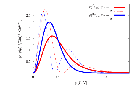
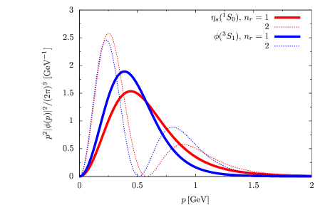
Figure 6: The single quark momentum distribution $p^{2}|\phi^{F,L}(p)|^{2}/(2\pi)^{3}\,[{\rm GeV}^{-1}]$ for $\pi\,(^{1}S_{0})$, $\rho\,(^{3}S_{1})$ states (upper panel) and $\eta_{s}\,(^{1}S_{0})$, $\phi\,(^{3}S_{1})$ states (lower panel). The radial excitations with $n_{r}=2$ are also shown in thin lines. The distributions for $s$-quarks are shifted slightly to higher momenta than for $ud$-quarks.

Figure 7: The momentum distribution $p^{2}|\phi(p)|^{2}\,[{\rm GeV}^{-1}]$ for the ${}^{2s+1}L_{j}=\,^{1}L_{L}$ states, $\pi\,(^{1}S_{0})$, $b_{1}\,(^{1}P_{1})$, and $\pi_{2}\,(^{1}D_{2})$ states.

Now we examine the quark momentum distributions in a hadron with $h=h^{JJ_{z}}_{LS}$ at rest (${\bm{P}}_{h}=0$). Shown in Fig.6 are the momentum distributions $p^{2}|\phi(p)|^{2}\,[{\rm GeV}^{-1}]$ for $\pi\,(^{1}S_{0})$, $\rho\,(^{3}S_{1})$ states (upper panel) and $\eta_{s}\,(^{1}S_{0})$, $\phi\,(^{3}S_{1})$ states (lower panel). The radial excitations with $n_{r}=2$ are also shown in thin lines. Due to the spin-spin attractions, $\pi$ is more compact than $\rho$, and hence tend to have higher momenta. In general, the $n_{r}$-th radial excitation has the distributions with $n_{r}$ peaks distributed from low to high momenta. We note that higher radial excitations contain more low momentum components than lower radial excitations. This is likely due to the broader spatial structure in higher radial excitations. The distributions for $s$-quarks are shifted slightly to higher momenta than for $ud$-quarks.

Shown in Fig.7 is the same as Fig.6 but for different states with ${}^{2s+1}L_{j}=\,^{1}L_{L}$ states, $\pi\,(^{1}S_{0})$, $b_{1}\,(^{1}P_{1})$, and $\pi_{2}\,(^{1}D_{2})$ states. Unlike the radial excitations, with a greater $L$ the distributions simply get shifted to higher momenta, and soft momentum components become smaller. The standard centrifugal barrier effects disfavor soft momentum components to develop.

V.3 Approximations for moving hadrons

To examine the properties of matter in hot and dense media, we need hadrons at finite momenta. At finite ${\bm{P}}_{h}$, several new elements enter: (i) in the relativistic treatments, the relative wavefunctions as functions of ${\bm{p}}_{r}$ generally also depend on ${\bm{P}}_{h}$ (the center of mass motion does not fully decouple); and (ii) we have to make an appropriate choice for $(c_{1},c_{2})$. The question is how the presence of a finite ${\bm{P}}_{h}$ affects our eigenvalue problem. Since our eigenvalue problems were not manifestly covariant, we compromise with some approximate treatments. For spectra, we simply assume $E({\bm{P}}_{h}=0)=m_{h}\rightarrow E({\bm{P}}_{h})=\sqrt{m_{h}^{2}+{\bm{P}}_{h}^{2}}$, without explicitly demonstrating it in our model. Meanwhile some extra discussions are needed for the wavefunctions. At this point we choose a specific combination of $(c_{1},c_{2})$ affect our eigenvalue problems including terms like $E_{1,2}=\sqrt{m_{1,2}^{2}+{\bm{p}}_{1,2}^{2}\,}$. One possible choice is to take

$$c_{ih}=\frac{\,\bar{E}_{i}\,}{\,\bar{E}_{1}+\bar{E}_{2}\,}=\frac{\,\bar{E}_{i}\,}{\,\bar{E}_{1+2}\,}\,,~{}~{}~{}~{}\bar{E}_{i}=\sqrt{m_{i}^{2}+\bar{{\bm{P}}}^{2}}\,,$$ (83)

where the subscript $h$ is attached to emphasize that $\bar{{\bm{P}}}^{2}$ depend on a meson being considered. The $c_{ih}$ gives $1/2$ in the equal mass case $(m_{1}=m_{2})$ or in the relativistic limit ($\bar{{\bm{P}}}^{2}/m_{i}^{2}\rightarrow\infty$), while leads to $m_{i}/(m_{1}+m_{2})$ in the non-relativistic limit ($\bar{{\bm{P}}}^{2}/m_{i}^{2}\rightarrow 0$). Substituting ${\bm{p}}_{1}=c_{1h}{\bm{P}}_{h}+{\bm{p}}$ and ${\bm{p}}_{2}=c_{2h}{\bm{P}}_{h}-{\bm{p}}$, and expanding in powers of ${\bm{P}}_{h}$ around ${\bm{P}}_{h}=0$, the $E_{1+2}$ term commonly appearing in our eigenvalue problem looks

$$E_{1+2}({\bm{P}}_{h})=E_{1+2}^{{\bm{P}}_{h}=0} + \bigg{(}\frac{c_{1h}}{\,E_{1}\,}-\frac{c_{2h}}{\,E_{2}\,}\bigg{)}\bigg{|}_{{\bm{P}}_{h}=0}{\bm{p}}\cdot{\bm{P}}_{h}$$ (84)

$$+ \bigg{(}\frac{c_{1h}^{2}}{\,E_{1}\,}+\frac{c_{2h}^{2}}{\,E_{2}\,}\bigg{)}\bigg{|}_{{\bm{P}}_{h}=0}\frac{\,{\bm{P}}_{h}^{2}\,}{\,2\,}+\cdots$$

Expanding $E_{i}$ in the denominator around $\bar{E}_{i}$, the cross term ${\bm{p}}\cdot{\bm{P}}_{h}$ vanishes, and

$$E_{1+2}({\bm{P}}_{h})\simeq E_{1+2}^{{\bm{P}}_{h}=0}+\frac{\,{\bm{P}}_{h}^{2}\,}{\,2\big{(}\bar{E}_{1}+\bar{E}_{2}\big{)}\,}+\cdots\,.$$ (85)

The way ${\bm{P}}_{h}^{2}$ appears is similar to what we would have for non-relativistic approximation for mesons, $E({\bm{P}}_{h})\simeq m_{h}+{\bm{P}}_{h}^{2}/2m_{h}+\cdots$. This motivates us to use $c_{i}$’s in Eq.(83), and the choice leads to the correct limiting behaviors in relativistic and non-relativistic limits. The quality of our approximation may be tested by comparing the above corrections in spectra with what we expect from the Poincare invariance, ${\bm{P}}_{h}^{2}/2m_{h}$. For ${\bm{P}}_{h}\ll\bar{E}_{1,2}$, we expect that it is a reasonable approximation to expand

$$\Psi_{{\bm{P}}_{h}}({\bm{p}})\simeq\Psi_{{\bm{P}}_{h}=0}({\bm{p}})+{\bm{P}}_{h}\cdot\partial_{{\bm{P}}_{h}}\Psi({\bm{p}})+\cdots\,,$$ (86)

as a weak external momentum does not affect internal wavefunctions characterized by hard momenta.

VI Meson resonance gas

Using the wavefunctions obtained so far, we compute the single quark momentum distributions $f^{T}_{{\bf q}}({\bm{p}})$ at a given temperature $T$ in a meson resonance gas (MRG). The distribution is compared to what we would obtain from percolated quarks extended over space.

VI.1 Quark occupation probability: formula

The $f_{\bf q}^{T}$ is computed by simply summing up the quark momentum distribution from each meson $h$ Kojo (2021a); Kojo and Suenaga (2022),

$$f_{\bf q}^{T}({\bm{p}})=\sum_{h}\int_{{\bm{P}}_{h}}n_{h}^{T}({\bm{P}}_{h})Q_{\rm in}^{h{\bf q}}({\bm{p}};{\bm{P}}_{h})\,,$$ (87)

where we assume the hadron $h$ with the energy $E_{h}({\bm{P}}_{h})=\sqrt{m_{h}^{2}+{\bm{P}}_{h}^{2}}$ obeys the Bose-Einstein distribution, $n_{h}^{T}({\bm{P}}_{h})=[\,\mathrm{e}^{E_{h}({\bm{P}}_{h})/T}-1\,]^{-1}$. The function $Q_{\rm in}^{h{\bf q}}({\bm{p}};{\bm{P}}_{h})$ specifies the distribution of a quark with the quantum number ${\bf q}$ and momentum ${\bm{p}}$, in a hadron $h$ with the momentum ${\bm{P}}_{h}$. Using the formula Eq.(65) for a single quark momentum distribution, we obtain

$$f_{\bf q}^{T}({\bm{p}}) = \sum_{h=h^{J}_{LS}}\int_{{\bm{P}}_{h}}n_{h}^{T}({\bm{P}}_{h})$$ (88)

$$\times\sum_{F,S_{z}}\frac{\,|b_{h}^{F}|^{2}\,}{\,N_{\rm c}\,}\,N_{{\bf q}SF}^{S_{z}}(2L+1)\,\frac{\,|\phi^{F,L}_{{\bm{P}}_{h}}(p_{r})|^{2}\,}{\,4\pi\,}\,,$$

where $p_{r}=|{\bm{p}}_{r}|$ with ${\bm{p}}_{r}={\bm{p}}-c_{1h}{\bm{P}}_{h}$, and the sum over $h=h^{J}_{LS}$ excludes the summation over $J_{z}$ which has been taken into account in the last factors of Eq.(88).

To treat this expression numerically, it is convenient to use ${\bm{k}}={\bm{p}}-c_{1h_{F}}{\bm{P}}_{h}$ as an integration variable where we update $h\rightarrow h_{F}$ to emphasize that $c_{1h}$ depends on the flavors $F$ in a hadron $h$; for instance $u$- and $s$-quarks in $\eta$ or $K$ have different $c_{1h}$. Using the approximation in Eq.(86),

$$f_{\bf q}^{T}({\bm{p}}) \simeq \sum_{h^{J}_{LS},F}\frac{1}{\,c_{1h_{F}}^{3}\,}\int_{{\bm{k}}}n_{h}^{T}\bigg{(}\frac{\,{\bm{p}}-{\bm{k}}\,}{c_{1h_{F}}}\bigg{)}$$ (89)

$$\times\sum_{S_{z}}\frac{\,|b_{h}^{F}|^{2}\,}{\,N_{\rm c}\,}\,N_{{\bf q}SF}^{S_{z}}(2L+1)\,\frac{\,|\phi^{F,L}_{{\bm{P}}_{h}=0}(k)|^{2}\,}{\,4\pi\,}\,.$$

The results presented below are based on this formula.

VI.2 Numerical results

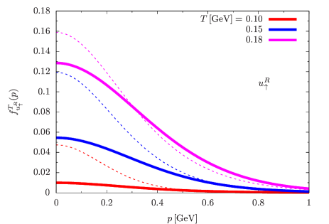
Figure 8: The occupation probabilities of single quark states, $f^{T}_{{\bf q}}(p)$, in our meson resonance gas model (bold lines) and in an ideal constituent quark gas (thin lines). The temperatures are $T=0.10,0.15$, and $0.18$ GeV. Results for the $u^{R}_{\uparrow}$ (upper panel) and $s^{R}_{\uparrow}$ (lower panel) states are shown. All the mesons up to $L=2$ and $n_{r}=3$ are included.

Figure 9: The occupation probabilities of $u^{R}_{\uparrow}$ (upper panel) and $s^{R}_{\uparrow}$ (lower panel) at $p=0$ as functions of temperature. The dashed lines are used for $f_{{\bf q}}^{\rm id}$. Solid curves are used for $f_{u^{R}_{\uparrow}}^{T}$. In the upper (lower) panel, we sequentially add pions (kaons), radial excitations up to $n_{r}=3$ for the $L=0,1$, and 2. The $ud$, $us$, $ss$ type mesons are included.

Now we numerically evaluate the integral in Eq.(89). We compare $f_{{\bf q}}^{T}$ in our MRG with the distribution for an ideal quark gas, $f_{\bf q}^{\rm id}=[\mathrm{e}^{E_{\bf q}({\bm{p}})/T}+1]^{-1}$, with the constituent quark masses same as used in our MRG, $M_{u}=0.30$ GeV and $M_{s}=0.48$ GeV. We regard the occupation probability of such a quark gas as that in a QGP, in the sense that quark states can be extended over space.

First we recall that the beginning of the crossover is $T\sim 150$ MeV in QCD where the HRG descriptions begin to break down. Another point to be kept in mind is that our model does not include baryons. (Meanwhile, the present results may be used to get some insights for two-color QCD where diquark baryons degenerate with mesons.) Keeping these insufficiencies in mind, we examine some trends in the following.

Shown in Fig.8 are the occupation probabilities of single quark states, $f^{T}_{{\bf q}}(p)$, in our MRG model (bold lines) and, $f_{\bf q}^{\rm id}$, in a QGP (thin lines). The temperatures are $T=0.10,0.15$, and $0.18$ GeV. Results for the $u^{R}_{\uparrow}$ (upper panel) and $s^{R}_{\uparrow}$ (lower panel) states are shown. All the mesons up to $L=2$ and $n_{r}=3$ are included.

At low temperatures, the $f_{\bf q}^{T}$ is lower than $f_{\bf q}^{\rm id}$ at low momenta. In the latter, the confining effects are absent so that quark wavefunctions can be widely extended, occupying low momentum states. As temperature increases, the number of hadrons increases drastically and quarks inside of such hadrons radically occupy low momentum states. The occupation probability at low momenta eventually exceeds $f_{\bf q}^{\rm id}$. Such temperature dependent evolution can be seen in Fig.9, where hadronic contributions are added sequentially to $f_{\bf q}^{T}(p)$ at $p=0$. In the upper (lower) panel for $f_{u^{R}_{\uparrow}}$ ($f_{s^{R}_{\uparrow}}$), only pions (kaons) with $n_{r}=1$ are included for the lowest curve; the next solid curve includes all $L=0$ hadronic states up to $n_{r}=3$, where $ud$, $us$, $ss$ type mesons are taken into account. We continue such adding to $L=2$. Around $T\sim 0.15$ GeV, the contributions from the radial excitations are substantial, as they include considerable $p=0$ components (Fig.6). The excess $f_{{\bf q}}^{T}$ over $f_{\bf q}^{\rm id}$ happens around $T\sim 0.2$ GeV. We emphasize that our MRG underestimates the true occupation probability which should be enhanced by baryons. If we include baryons, the $f_{{\bf q}}^{T}$ should exceed $f_{{\bf q}}^{\rm id}$ at lower temperature, perhaps somewhere around $0.15$-$0.18$ GeV.

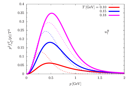
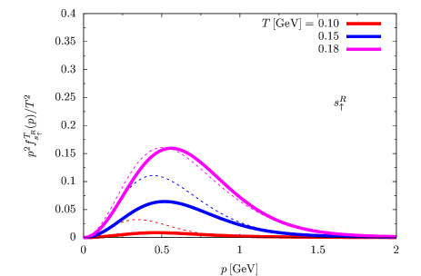
Figure 10: The same as Fig.8 but the factor $p^{2}/T^{2}$ is multiplied.

To examine which momentum states are typical, it is useful to multiply the phase space factor $4\pi p^{2}$. Shown in Fig.10 are the same as Fig.8 but a factor $p^{2}/T^{2}$ is multiplied. At $T=0.10$ GeV, it is clear that quarks inside of hadrons have substantially larger occupation probability for high momentum states than the ideal quark gas case. This excess in $f^{T}_{{\bf q}}$ at high momenta is expected to decrease as quarks gradually percolate; for hadrons greater in size have more chances to accommodate extended, low momentum quark states. Such extended states in hadrons are partially taken into account through radially excited states with $n_{r}>1$ which contain substantial low momentum states as seen in Fig.6.

VI.3 Discussions

VI.3.1 Dissociations of hadrons

We have been interested in how the effective degrees of freedom transform from hadronic to hot and dense phases. For such transitions to occur smoothly, the properties of quarks in a HRG and a QGP should be close.

We infer that quark states in a HRG tend to have less probability at low momenta but greater probability at higher momenta than in a QGP, as they are packed into hadrons with the finite size. Although we still did not include baryons, we have observed such trend at low temperature $T\lesssim 0.15$ GeV in Figs.9 and 10.

Meanwhile, at higher temperatures, $f_{{\bf q}}$ in a HRG begins to exceed the QGP counterpart from low to high momenta. We suspect that such overall excess in a HRG is an artifact of extrapolating the ideal gas picture of hadrons. When hadrons overlap significantly, we expect that quarks percolate, occupying low momentum states. Based on this picture, we expect the followings to happen:

(i) Hadrons with large radii preferentially merge, and form media filled by color electric fluxes (string condensations Polyakov (1978)).

(ii) Having colored backgrounds, quarks may be extended in space. This induces the decay of hadrons at large size into quarks and antiquarks which can get bound to colored backgrounds. Such percolation enhances the occupation probability at low momenta while reduces the number of high momentum states.

(iii) The decays of highly excited hadrons reduce the hadronic contributions to the thermodynamics, tempering the drastic growth in thermodynamic quantities, e.g., entropies as in Hagedörn’s gas Hagedorn (1965); Broniowski et al. (2004). Such dissociation also tempers the rapid growth in the quark occupation probabilities. More precisely, the correct treatment of the decays leads to not only vanishing contributions from decaying hadrons, but also results in the negative contributions to the thermodynamics Dashen et al. (1969); Blaschke et al. (2014, 2015); Lo (2017); Cleymans et al. (2021). Such decay channels open at high energy, canceling the positive contributions from ordinary resonances at lower energy. Eventually the thermodynamics is dominated by elementary particles.

We a bit more elaborate the negative contributions just mentioned above. For the channel $X$ in two-body problems, the thermodynamic pressure may be expressed using the phase shift $\delta_{X}$ as Dashen et al. (1969); Blaschke et al. (2014, 2015); Lo (2017)

$$P_{\rm th}^{X}=-\int_{{\bm{p}}}\int_{0}^{\infty}\frac{\,\mathrm{d}\omega\,}{\,\pi\,}T\ln\big{(}1-\mathrm{e}^{-\omega/T}\big{)}\frac{\,\mathrm{d}\delta_{X}(\omega,{\bm{p}})\,}{\,\mathrm{d}\omega\,}\,,$$ (90)

where the phase shift obeys the constraint from Levinson’s theorem,

$$\int_{\bm{p}}\big{[}\,\delta_{X}(\omega=\infty,{\bm{p}})-\delta_{X}(\omega=0,{\bm{p}})\,\big{]}=0\,.$$ (91)

The physical meaning of this theorem is that interactions cannot change the size of the Hilbert space. For an ideal meson gas, the phase shift is

$$\delta_{X}^{\rm id}(\omega,{\bm{p}})=\sum_{n}\pi\theta\big{(}\,\omega-E_{n}({\bm{p}})\,\big{)}\,,$$ (92)

with which we get the sum of mesonic excitations for Eq.(90). Actually this expression is inconsistent with the Levinson’s theorem, as the $\delta_{X}$ keeps growing with $\omega$. The correct phase shift, which carries the information that resonances are made of elementary particles, decreases when the continuum is opened at high energy. The phase at $\omega=0$ is $\delta_{X}(\omega=0)=0$, and must eventually approach zero at $\omega\rightarrow\infty$. Such domains at high energy show up in thermodynamics at very high temperature, yielding the negative contributions which cancel the resonance contributions at lower energy. For model studies, see, e.g., Refs.Blaschke et al. (2014, 2015) in the context of HRG to QGP transitions.

As we have seen through the Levinson’s theorem, it is in general important to handle double counting of contributions from composite particles and elementary particles. One of systematic frameworks which automatically handle such double counting is the $\Phi$-derivable approach Baym (1962) or the two-particle-irreducible (2PI) formalism Cornwall et al. (1974). In particular the zero temperature contributions would be UV divergent unless we properly handle the double counting problem, see, e.g., Ref.Kojo (2020) in the context of equations of state with quark-hadron continuity; with proper treatments of double counting, the apparent UV divergences from baryonic contributions and those from quark contributions are assembled to cancel.

VI.3.2 Large $N_{\rm c}$, overlap of hadrons, and percolation

Intuitively the overlap of hadrons is supposed to lead to percolation of quarks, but we should be more precise here. To illustrate the points, here we consider QCD with large number of colors. In such theories interactions among mesons are $\sim 1/N_{\rm c}$ and suppressed ’t Hooft (1974); Witten (1979a), while baryons have the masses of $\sim N_{\rm c}$ Hidaka et al. (2008), too massive to participate in the thermodynamics at $T\sim\Lambda_{\rm QCD}$. The usual conjecture is that the deconfinement happens as the first order transitions, in the same way as in pure Yang-Mills theories at $N_{\rm c}>2$ when gluons saturate the space Panero (2009). In pure-Yang Mills at $N_{\rm c}=3$, the deconfinement temperature is $T_{\rm YM}\simeq 0.26$ GeV Boyd et al. (1996), considerably larger than the case with quarks, $T\simeq 0.15$ GeV, where the entropy is $s\sim 2$-3 fm^-3 indicating the overlap of hadrons with the radii $\sim 1$ fm.

In large $N_{\rm c}$, the spatial overlap of mesons is supposed to be insensitive to $N_{\rm c}$, but depends only on the size of mesons characterized by $\Lambda_{\rm QCD}$. Provided that the above argument for meson sizes and $T_{\rm QCD}\rightarrow T_{\rm YM}$ at large $N_{\rm c}$, we have to conclude that the overlap of hadrons are not sufficient to drive the deconfinement or percolation of quarks. We need a stronger condition. With meson-meson interactions of $\sim N_{\rm c}^{-1}$, the transformations of effective degrees of freedom, from hadrons to quarks, happen only after the meson abundance becomes large enough to compensate the $1/N_{\rm c}$ suppression of interactions.

In order to keep track of quarks from a HGP to a QGP, it is useful to look at the quark occupation probability in hadrons. The probability to find a quark with a given color is $\sim 1/N_{\rm c}$, and its magnitude is significantly smaller that that from percolating quarks where there is no suppression factor of $1/N_{\rm c}$. This disparity is resolved only when drastic increase in the number of hadrons occurs to compensate the $1/N_{\rm c}$ suppression.

Let us estimate the magnitude of meson exchange interactions between mesons, using the quark-meson vertices $g_{qqM}$ which are known to be $\sim N_{\rm c}^{-1/2}$. At low temperature where the meson abundance is $O(1)$ and hence $f_{{\bf q}}\sim N_{\rm c}^{-1}$, the magnitudes of interactions in a HRG are

$$N_{\rm c}^{2}\big{(}f^{{\rm low}\,T}_{{\bf q}}\big{)}^{2}g_{qqM}^{2}\sim N_{\rm c}^{2}(N_{\rm c}^{-1})^{2}(N_{\rm c}^{-1/2})^{2}\sim N_{\rm c}^{-1}\,,$$ (93)

where we include the combinatorics to pick up quark colors, $\sim N_{\rm c}^{2}$. Thus the interactions in the thermodynamics are negligible compared to the ideal meson gas contributions of $O(1)$.

At higher temperature, the interactions become comparable to the ideal gas contributions when the meson abundance reaches $O(N_{\rm c})$ due to highly excited states. (With such large abundance, the ideal gas contributions to the thermodynamic potential also become $O(N_{\rm c})$.) In the purely mesonic language, the meson three point vertices are $\sim N_{\rm c}^{-1/2}$, and the interactions are

$$N_{\rm c}^{2}\big{(}N_{\rm c}^{-1/2}\big{)}^{2}\sim N_{\rm c}\,,$$ (94)

which is comparable to the ideal meson gas contribution of $\sim N_{\rm c}$. The equivalent descriptions are possible by noting that the meson abundance of $\sim N_{\rm c}$ leads to $f^{{\rm high}\,T}_{{\bf q}}\sim 1$. Then the magnitude of the interactions among quarks is

$$N_{\rm c}^{2}\big{(}f^{{\rm high}\,T}_{{\bf q}}\big{)}^{2}g_{qqM}^{2}\sim N_{\rm c}^{2}1^{2}(N_{\rm c}^{-1/2})^{2}\sim N_{\rm c}\,,$$ (95)

which is the magnitude expected from a percolated quark gas. The corresponding thermodynamic potential is $\sim N_{\rm c}$. Here mesonic and quark gas descriptions should have some overlap in the domain of validity. This regime holds before the temperature reaches $T_{\rm YM}$ where the thermodynamic potential is $\sim N_{\rm c}^{2}$. We note that the $f^{T}_{{\bf q}}$ is bound from above, $f_{{\bf q}}^{T}\leq 1$, so that the quark contribution to the thermodynamics cannot exceed $\sim N_{\rm c}$; diverging behaviors in Hagedörn’s gas are tempered by the quark substructure of hadrons, at least for resonances made of quarks.

VII Summary

In this work we study a relativistic constituent quark model which is arranged for the studies of the quark-hadron continuity in hot and dense matter. We analyze mesons including quarks from light to charm quark sectors. The spectra are reproduced within $\sim$5-10% accuracy, up to the energy of $\sim 2.5$ GeV. The impacts of relativistic kinematics, scalar vs vector confinement, and short range correlations are examined. At conceptual level, considerable differences from the non-relativistic counterpart are found in all these effects. After obtaining quark wavefunctions, we calculate the occupation probability of quark states in an ideal meson gas. In order to get insights on the transformation of effective degrees of freedom from a HRG to a QGP, we compare the occupation probabilities of quark states in a HRG with those in a QGP.

Although we still have to compute baryonic contributions to complete our HRG descriptions for quarks, we think that the behaviors of quark occupation probabilities are reasonable in the magnitudes and shapes. It may be possible to consider a regime where hadrons overlap but the interactions are still tractable in expansion of $1/N_{\rm c}$. Whether one can use such a regime to describe the continuous transformation of effective degrees of freedom is an interesting future subject.

Clearly many aspects in the present paper remain to be improved and extended:

(i) The obvious thing to do is the computations of baryon wavefunctions and the corresponding quark occupation probabilities. Such computations will complete our descriptions of a HRG. Furthermore, the quark momentum distributions in a baryon have direct impacts on descriptions for cold, dense nuclear matter beyond the nuclear saturation regime Kojo (2021a); Kojo and Suenaga (2022).

(ii) We think that parameters used for hadron spectra can be more systematically explored, employing the bayesian or deep learning approaches. The determination of parameters for inner quark dynamics, e.g., $\alpha_{s}$, is important by its own. We should also include more experimental data to get stronger constraints on the model space.

(iii) It is important to calculate the hadron-hadron interaction vertices using the quark wavefunctions. The hadronic interactions are related to the underlying hadronic structures which may change in medium. Such information is relevant in descriptions of baryon rich matters in heavy ion collisions at low and intermediate energies and in neutron stars.

In addition, the framework in this paper should be also tested in QCD-like theories. For instance, for QCD in magnetic fields, some lattice results and model studies have been available for the structural changes in hadrons Andreichikov et al. (2017); Hattori and Yamamoto (2019); Kojo (2021c); Hattori et al. (2016); Kojo and Su (2013); Endrődi and Markó (2019); Mao (2016); Fukushima and Hidaka (2013). Also isospin QCD Son and Stephanov (2001); Splittorff et al. (2001); He et al. (2005); Cohen and Sen (2015); Brandt et al. (2018a, b); Adhikari et al. (2018); Adhikari and Andersen (2020) and two-color QCD Kogut et al. (1999); Ratti and Weise (2004); Brauner et al. (2009); Boz et al. (2020); Begun et al. (2022); Iida et al. (2020, 2021) have lattice QCD simulations and are important test-beds. In particular, both mesons and baryons in two-color QCD are calculated within two-body framework, so that some predictions can be readily made from the results obtained in the present paper. The results will be reported elsewhere.

Appendix A Coordinate space form factors

In Eq.(31) we have introduced a form factor for each quark-gluon vertex. The form factor removes artificial short distance singularities arising from a replacement $\sim{\bm{k}}/E\rightarrow{\bm{k}}/\bar{E}$ where the ${\bm{k}}$-dependence in the denominator is neglected. The replacement should be valid for $|{\bm{k}}|\ll\bar{E}$, so we limit the domain of the approximation by multiplying the factors from the vertices 1 and 2,

$$F({\bm{k}})=\mathrm{e}^{-{\bm{k}}^{2}\big{(}\Lambda_{v1}^{-2}+\Lambda_{v2}^{-2}\big{)}}=\mathrm{e}^{-{\bm{k}}^{2}\Lambda_{v}^{-2}}\,,$$ (96)

where $\Lambda_{v1,2}$ is $\sim\bar{E}_{1,2}$. Meanwhile the large momentum contributions of $|{\bm{k}}|\gg\bar{E}$ are assumed to be used to renormalize effective model parameters. Thus such components are simply neglected.

With these form factors, the potentials convoluted with the vertex factors are now treated as

$$\!\!\!\frac{\,(\mathrm{i}k_{i}\cdots)\,}{\,f(E_{1})f(E_{2})\,}U({\bm{k}})~{}\rightarrow~{}\frac{\,(\mathrm{i}k_{i}\cdots)\,}{\,f(\bar{E}_{1})f(\bar{E}_{2})\,}F({\bm{k}})U({\bm{k}})\,.$$ (97)

Next we take the Fourier transform into the coordinate space expression,

$$(\mathrm{i}k_{i}\cdots)F({\bm{k}})U({\bm{k}})~{}\rightarrow~{}(\partial_{i}\cdots)\int_{{\bm{R}}}F({\bm{r}}-{\bm{R}})U({\bm{R}})$$

$$~{}~{}~{}~{}~{}~{}~{}~{}~{}~{}~{}~{}~{}~{}=(\partial_{i}\cdots)\int_{0}^{\infty}\!\!\mathrm{d}R~{}G(r,R)U(R)\,,$$ (98)

with a function regular at small $r$ (we set $\beta=\Lambda_{v}/2$),

$$\!\!\!\!\!G(r,R)=\frac{\,\beta\,}{\,\sqrt{\pi}\,}\frac{\,R\,}{r}\bigg{[}\,\mathrm{e}^{-\beta^{2}(r-R)^{2}}-\mathrm{e}^{-\beta^{2}(r+R)^{2}}\bigg{]}\,.$$ (99)

The derivatives $(\partial_{i}\cdots)$ hit only $G(r,R)$ so that one can prepare formulae for $(\partial_{i}\cdots)G(r,R)$ and simply convolute it with any $U(R)$.

The expressions Eqs.(98) and (99) are already tractable numerically, but we further simplify the expression by extracting the asymptotic behaviors at large $r$ and small $r$, and then by interpolating those analytic expressions.

At small $r$, the first and second terms in $G(r,R)$ tend to largely cancel. For $r\ll\Lambda_{v}^{-1}$

$$\int_{0}^{\infty}\!\!\mathrm{d}R~{}G(r,R)U(R)~{}\simeq~{}\mathrm{e}^{-\beta^{2}r^{2}}U_{\rm sh}$$ (100)

where $U_{\rm sh}$ is the average potential energy in a volume $\beta^{-3}$,

$$U_{\rm sh}\equiv\frac{\,4\beta^{3}\,}{\,\sqrt{\pi}\,}\,\int_{0}^{\infty}\mathrm{d}R\,\mathrm{e}^{-\beta^{2}R^{2}}R^{2}U(R)\,.$$ (101)

For $U_{\rm OGE}(r)=-4\alpha_{s}/3r$,

$$U_{\rm OGE}^{\rm sh} = \frac{\,2\,}{\,\sqrt{\pi}\,}\bigg{(}-\frac{\,4\,}{\,3\,}\alpha_{s}\beta\bigg{)}=\frac{\,2\,}{\,\sqrt{\pi}\,}U_{\rm OGE}(\beta^{-1})\,,$$ (102)

and for $U_{\rm conf}^{S,V}(r)=f_{S,V}\times\sigma r$,

$$(U_{\rm conf}^{S,V})^{\rm sh}=\frac{\,2\,}{\,\sqrt{\pi}\,}\bigg{(}f_{S,V}\frac{\,\sigma\,}{\,\beta\,}\bigg{)}=\frac{\,2\,}{\,\sqrt{\pi}\,}U_{\rm conf}^{S,V}(\beta^{-1})\,.$$ (103)

It turns out that these expressions can be obtained by substituting $\beta^{-1}$ in place of $r$ of the potentials and multiplying a factor $2/\sqrt{\pi}$.

To summarize, our approximation proceeds as follows,

$$\!\!\!\frac{\,(\mathrm{i}k_{i}\cdots)\,}{\,f(E_{1})f(E_{2})\,}U({\bm{k}})~{}\rightarrow~{}\frac{\,(\mathrm{i}k_{i}\cdots)\,}{\,f(\bar{E}_{1})f(\bar{E}_{2})\,}U_{\rm reg}(r)\,,$$ (104)

with $U_{\rm reg}$ interpolating analytic expressions for short and large distance,

$$U_{\rm reg}=\mathrm{e}^{-\beta^{2}r^{2}}U_{\rm sh}\,,$$ (105)

as given in Eq.(33).

Appendix B Potentials with derivatives

We use the following notations for our replacement procedures,

$$(\mathrm{i}{\bm{k}})_{i}(\mathrm{i}{\bm{k}})_{j}\tilde{U}~{} \rightarrow ~{}\delta_{ij}\bar{U}_{2}(r)/3+Q_{ij}\bar{U}_{2T}(r)/3\,,$$

$$(\mathrm{i}{\bm{k}}\times{\bm{P}})\tilde{U}~{} \rightarrow ~{}{\bm{L}}\bar{U}_{1L}(r)\,,$$

$$(\mathrm{i}{\bm{k}}\times{\bm{P}})_{i}(\mathrm{i}{\bm{k}}\times{\bm{P}})_{j}\tilde{U}~{} \rightarrow ~{}\mathcal{P}_{ij}\bar{U}_{2\mathcal{P}}(r)+L_{i}L_{j}\bar{U}_{2L^{2}}(r)\,,$$

where we have defined

$$\mathcal{P}_{ij}=\delta_{ij}{\bm{P}}^{2}-P_{i}P_{j}\,,~{}~{}~{}Q_{ij}=\delta_{ij}-\frac{\,3x_{i}x_{j}\,}{\,r^{2}\,}\,.$$ (107)

The subscript of $\bar{U}$ indicates the powers of ${\bm{k}}$. Explicitly, each potential is computed from $U_{\rm reg}$ as

$$\bar{U}_{2}={\bm{\nabla}}^{2}U_{\rm reg}\,,~{}~{}~{}~{}\bar{U}_{2T}=-\bigg{(}\frac{\,\mathrm{d}^{2}\,}{\,\mathrm{d}r^{2}\,}-\frac{1}{\,r\,}\frac{\,\mathrm{d}\,}{\,\mathrm{d}r\,}\bigg{)}U_{\rm reg}\,,$$

$$~{}~{}~{}~{}~{}~{}~{}~{}~{}\bar{U}_{1L}(r)=\bar{U}_{2\mathcal{P}}(r)=\frac{1}{\,r\,}\frac{\,\mathrm{d}U_{\rm reg}\,}{\,\mathrm{d}r\,}\,,$$

$$~{}~{}~{}~{}~{}~{}~{}\bar{U}_{2L^{2}}(r)=\frac{1}{\,r^{2}\,}\bigg{(}\frac{\,\mathrm{d}^{2}\,}{\,\mathrm{d}r^{2}\,}-\frac{1}{\,r\,}\frac{\,\mathrm{d}\,}{\,\mathrm{d}r\,}\bigg{)}U_{\rm reg}\,.$$ (108)

It is useful to note

$${\bm{\nabla}}^{2}U_{\rm reg}=2\beta^{2}(-3+2\beta^{2}r^{2})\mathrm{e}^{-\beta^{2}r^{2}}U_{\rm sh}\,.$$ (109)

$$\bigg{(}\frac{\,\mathrm{d}^{2}\,}{\,\mathrm{d}r^{2}\,}-\frac{1}{\,r\,}\frac{\,\mathrm{d}\,}{\,\mathrm{d}r\,}\bigg{)}U_{\rm reg}=4\beta^{4}r^{2}\mathrm{e}^{-\beta^{2}r^{2}}\,U_{\rm sh}\,.$$ (110)

$$\frac{\,\mathrm{d}U_{\rm reg}\,}{\,\mathrm{d}r\,}=-2\beta^{2}r\mathrm{e}^{-\beta^{2}r^{2}}U_{\rm sh}\,.$$ (111)

Appendix C Color-flavor-spin factors

Here we summarize factors related to the spin and flavor wavefunctions. For non-flavored mesons, we basically assume the ideal mixing which separates $ud$ and $s$-quark sectors, e.g., $\omega\sim u\bar{u}+d\bar{d}$ and $\phi\sim s\bar{s}$. Only the $\eta$ mesons are treated differently, $\eta\sim u\bar{u}+d\bar{d}-2s\bar{s}$, as they appear in the low mass region.

First we discuss the factors $b_{h}^{F}$. Here we list only the $b_{h}^{F}$’s which are nonzero. For $\mathcal{I}=0$ states purely made of $ud$-quarks (e.g., $\omega$),

$$b_{\mathcal{I}=0,ud}^{u\bar{u}}=b_{\mathcal{I}=0,ud}^{d\bar{d}}=1/\sqrt{2}\,.$$ (112)

For $\mathcal{I}=1$ states (e.g., $\pi$, $\rho$),

$$b_{\mathcal{I}_{3}=0}^{u\bar{u}}=-b_{\mathcal{I}_{3}=0}^{d\bar{d}}=1/\sqrt{2}\,,~{}~{}~{}b_{\mathcal{I}_{3}=1}^{u\bar{d}}=b_{\mathcal{I}_{3}=-1}^{d\bar{u}}=1\,.$$ (113)

For $\mathcal{I}=1/2$ states (e.g., $K$),

$$b_{\mathcal{I}_{3}=1/2}^{u\bar{s}}=b_{\mathcal{I}_{3}=1/2}^{s\bar{d}}=b_{\mathcal{I}_{3}=-1/2}^{s\bar{u}}=b_{\mathcal{I}_{3}=-1/2}^{d\bar{s}}=1\,.$$ (114)

For $\mathcal{I}=0$ states purely made of $s$-quarks (e.g., $\phi$),

$$b_{\mathcal{I}=0,s}^{s\bar{s}}=1\,.$$ (115)

Finally, for $\eta$,

$$b_{\eta}^{u\bar{u}}=b_{\eta}^{d\bar{d}}=1/\sqrt{6}\,,~{}~{}~{}~{}~{}b_{\eta}^{d\bar{d}}=-2/\sqrt{6}\,.$$ (116)

Next we discuss $N_{{\bf q}SF}^{S_{z}}$. Here we pick up $u^{R}_{\uparrow}$ for definiteness. The only nonzero components are

$$N_{u^{R}_{\uparrow}S(u\bar{u})}^{S_{z}}=N_{u^{R}_{\uparrow}S(u\bar{d})}^{S_{z}}=N_{u^{R}_{\uparrow}S(u\bar{s})}^{S_{z}}=N_{q_{\uparrow}S}^{S_{z}}\,,$$ (117)

where

$$N_{q_{\uparrow}S=1}^{S_{z}=1}=1\,,~{}~{}~{}~{}N_{q_{\uparrow}S=1}^{S_{z}=-1}=0\,,~{}~{}~{}~{}$$

$$N_{q_{\uparrow}S=1}^{S_{z}=0}=N_{q_{\uparrow}S=0}^{S_{z}=0}=1/2\,.$$ (118)

Finally we show some examples for terms in our HRG model, Eq.(80). Setting ${\bf q}=u^{R}_{\uparrow}$,

$$\sum_{J_{z}}Q_{\rm in}^{hu^{R}_{\uparrow}}=\frac{\,1\,}{\,N_{\rm c}\,}\sum_{F,S_{z}}|b_{h}^{F}|^{2}\,N_{u^{R}_{\uparrow}SF}^{S_{z}}\,\frac{\,|\phi^{F}_{{\bm{P}}_{h}}(p)|^{2}\,}{4\pi}\,.$$ (119)

For $\pi$,

$$Q_{\rm in}^{\pi_{0}u^{R}_{\uparrow}} = \frac{\,1\,}{\,N_{\rm c}\,}\frac{1}{\,2^{2}\,}\,\frac{\,|\phi^{ud}_{{\bm{P}}_{h}}(p)|^{2}\,}{4\pi}\,,$$

$$Q_{\rm in}^{\pi_{+}u^{R}_{\uparrow}} = \frac{\,1\,}{\,N_{\rm c}\,}\frac{1}{\,2\,}\,\frac{\,|\phi^{ud}_{{\bm{P}}_{h}}(p)|^{2}\,}{4\pi}\,,$$

$$Q_{\rm in}^{\pi_{-}u^{R}_{\uparrow}} = 0\,.$$ (120)

For $K$, setting ${\bf q}=u^{R}_{\uparrow}$,

$$Q_{\rm in}^{K_{+}u^{R}_{\uparrow}}=\frac{\,1\,}{\,N_{\rm c}\,}\frac{1}{\,2\,}\,\frac{\,|\phi^{us}_{{\bm{P}}_{h}}(p)|^{2}\,}{4\pi}\,,$$

$$Q_{\rm in}^{\bar{K}_{0}u^{R}_{\uparrow}}=Q_{\rm in}^{K_{-}u^{R}_{\uparrow}}=Q_{\rm in}^{K_{0}u^{R}_{\uparrow}}=0\,.$$ (121)

or setting ${\bf q}=s^{R}_{\uparrow}$,

$$Q_{\rm in}^{K_{-}s^{R}_{\uparrow}}=Q_{\rm in}^{K_{0}u^{R}_{\uparrow}} = \frac{\,1\,}{\,N_{\rm c}\,}\frac{1}{\,2\,}\,\frac{\,|\phi^{us}_{{\bm{P}}_{h}}(p)|^{2}\,}{4\pi}\,,$$

$$Q_{\rm in}^{K_{+}s^{R}_{\uparrow}}=Q_{\rm in}^{\bar{K}_{0}s^{R}_{\uparrow}} = 0\,.$$ (122)

For $\eta$,

$$Q_{\rm in}^{\eta u^{R}_{\uparrow}} = \frac{\,1\,}{\,N_{\rm c}\,}\frac{\,1\,}{\,12\,}\frac{\,|\phi^{ud}_{{\bm{P}}_{h}}(p)|^{2}\,}{4\pi}\,,$$

$$Q_{\rm in}^{\eta s^{R}_{\uparrow}} = \frac{\,1\,}{\,N_{\rm c}\,}\frac{\,1\,}{\,3\,}\frac{\,|\phi^{us}_{{\bm{P}}_{h}}(p)|^{2}\,}{4\pi}\,.$$ (123)

For $\rho$,

$$\sum_{J_{z}}Q_{\rm in}^{\rho_{0}u^{R}_{\uparrow}} = \frac{\,1\,}{\,N_{\rm c}\,}\frac{3}{\,2^{2}\,}\,|\phi^{ud}_{{\bm{P}}_{h}}(p)|^{2}\,,$$

$$\sum_{J_{z}}Q_{\rm in}^{\rho_{+}u^{R}_{\uparrow}} = \frac{\,1\,}{\,N_{\rm c}\,}\frac{3}{\,2\,}\,|\phi^{ud}_{{\bm{P}}_{h}}(p)|^{2}\,,$$

$$\sum_{J_{z}}Q_{\rm in}^{\rho_{-}u^{R}_{\uparrow}} = 0\,.$$ (124)

For $\phi$, we consider ${\bf q}=s^{R}_{\uparrow}$,

$$\sum_{J_{z}}Q_{\rm in}^{\phi s^{R}_{\uparrow}} = \frac{\,1\,}{\,N_{\rm c}\,}\frac{3}{\,2\,}\,|\phi^{ss}_{{\bm{P}}_{h}}(p)|^{2}\,.$$ (125)

As should be already clear, the sum over isospin yields the factor $2\mathcal{I}+1$. For $\mathcal{I}\neq 0$, we can use the formula

$$\sum_{\mathcal{I}_{z},J_{z}}Q_{\rm in}^{h{\bf q}}=\frac{\,(2L+1)(2S+1)(2\mathcal{I}+1)\,}{\,4N_{\rm c}\,}|\phi^{f}_{{\bm{P}}_{h}}(p)|^{2}\,.$$ (126)

where $f=ud$ or $us$. For $\mathcal{I}=0$ states purely made of $ud$,

$$\sum_{J_{z}}Q_{\rm in}^{h{\bf q}}=\frac{\,(2L+1)(2S+1)\,}{\,4N_{\rm c}\,}|\phi^{ud}_{{\bm{P}}_{h}}(p)|^{2}\,,$$ (127)

and states purely made of $s$,

$$\sum_{J_{z}}Q_{\rm in}^{h{\bf q}}=\frac{\,(2L+1)(2S+1)\,}{\,2N_{\rm c}\,}|\phi^{ss}_{{\bm{P}}_{h}}(p)|^{2}\,.$$ (128)

Appendix D Fourier transform

We discuss how to calculate $\phi_{L}(k)$ from our coordinate space wavefunctions, including the normalization factor. Our definition of $\phi_{L}(k)$ comes from

$$\langle{\bm{k}}|\Psi_{L}^{L_{z}}\rangle=\phi_{L}(k)Y_{L}^{L_{z}}(\hat{{\bm{k}}})\,,$$ (129)

The normalization condition leads to

$$\int_{\bm{k}}|\Psi_{L}^{L_{z}}({\bm{k}})|^{2}=1~{}\rightarrow\int_{0}^{\infty}\!\!\!\mathrm{d}k\,k^{2}|\phi_{L}(k)|^{2}=(2\pi)^{3}\,.$$ (130)

To relate $\phi_{L}(k)$ and $\phi_{L}(r)$, it is convenient to choose $|{\bm{k}}\rangle=|k,{\bm{n}}_{z}\rangle$ where ${\bm{n}}_{z}$ is the quantization axis of $(L,L_{z})$. Then, the angle between ${\bm{k}}$ and ${\bm{r}}$ is the same as the angle appearing in the spherical functions. We now evaluate

$$\langle k,{\bm{n}}_{z}|\Psi_{L}^{L_{z}}\rangle=\int_{{\bm{r}}}\langle k,{\bm{n}}_{z}|{\bm{r}}\rangle\langle{\bm{r}}|\Psi_{L}^{L_{z}}\rangle$$

$$=2\pi\delta_{L_{z},0}\sum_{L^{\prime}}\mathrm{i}^{L^{\prime}}(2L^{\prime}+1)\int\mathrm{d}rr^{2}\,j_{L^{\prime}}(kr)\phi_{L}(r)$$

$$~{}~{}~{}~{}~{}~{}~{}~{}~{}\times\int\mathrm{d}\cos\theta~{}P_{L^{\prime}}(\cos\theta)P_{L}(\cos\theta)\sqrt{\frac{\,2L+1\,}{\,4\pi\,}}$$

$$=\mathrm{i}^{L}\delta_{L_{z},0}\sqrt{4\pi(2L+1)\,}\,\int\mathrm{d}rr^{2}\,j_{L^{\prime}}(kr)\phi_{L}(r)\,.$$ (131)

where $j_{L}$ is the spherical Bessel function and $P_{L}$ Legendre functions. Meanwhile

$$\langle k,{\bm{n}}_{z}|\Psi_{L}^{L_{z}}\rangle=\phi_{L}(k)Y_{L}^{L_{z}}({\bm{n}}_{z})=\phi_{L}(k)\delta_{0}^{L_{z}}\sqrt{\frac{\,2L+1\,}{\,4\pi\,}}\,,$$

so that

$$\phi_{L}(k)=4\pi\int\mathrm{d}rr^{2}\,j_{L}(kr)\phi_{L}(r)\,.$$ (133)

References

- ’t Hooft (1974) Gerard ’t Hooft, “A Planar Diagram Theory for Strong Interactions,” Nucl. Phys. B 72, 461 (1974).
- Witten (1979a) Edward Witten, “Baryons in the 1/n Expansion,” Nucl. Phys. B 160, 57–115 (1979a).
- Fukushima et al. (2020) Kenji Fukushima, Toru Kojo, and Wolfram Weise, “Hard-core deconfinement and soft-surface delocalization from nuclear to quark matter,” Phys. Rev. D 102, 096017 (2020), arXiv:2008.08436 [hep-ph] .
- Yukawa (1935) Hideki Yukawa, “On the Interaction of Elementary Particles I,” Proc. Phys. Math. Soc. Jap. 17, 48–57 (1935).
- Nambu (1957) Yoichiro Nambu, “Possible existence of a heavy neutral meson,” Phys. Rev. 106, 1366–1367 (1957).
- Sakurai (1960) J. J. Sakurai, “Spin-orbit force and a neutral vector meson,” Phys. Rev. 119, 1784–1785 (1960).
- Stoks et al. (1994) V. G. J. Stoks, R. A. M. Klomp, C. P. F. Terheggen, and J. J. de Swart, “Construction of high-quality nn potential models,” Phys. Rev. C 49, 2950–2962 (1994).
- Machleidt et al. (1996) R. Machleidt, F. Sammarruca, and Y. Song, “Nonlocal nature of the nuclear force and its impact on nuclear structure,” Phys. Rev. C 53, R1483–R1487 (1996).
- Hatsuda (2018) Tetsuo Hatsuda, “Lattice quantum chromodynamics and baryon-baryon interactions,” Front. Phys. (Beijing) 13, 132105 (2018).
- Park et al. (2020) Aaron Park, Su Houng Lee, Takashi Inoue, and Tetsuo Hatsuda, “Baryon–baryon interactions at short distances: constituent quark model meets lattice QCD,” Eur. Phys. J. A 56, 93 (2020), arXiv:1907.06351 [hep-ph] .
- Oka and Yazaki (1980) M. Oka and K. Yazaki, “Nuclear Force in a Quark Model,” Phys. Lett. B 90, 41–44 (1980).
- Oka and Yazaki (1981a) M. Oka and K. Yazaki, “Short Range Part of Baryon Baryon Interaction in a Quark Model. 2. Numerical Results for S-Wave,” Prog. Theor. Phys. 66, 572–587 (1981a).
- Oka and Yazaki (1981b) M. Oka and K. Yazaki, “Short Range Part of Baryon Baryon Interaction in a Quark Model. 1. Formulation,” Prog. Theor. Phys. 66, 556–571 (1981b).
- McLerran and Pisarski (2007) Larry McLerran and Robert D. Pisarski, “Phases of cold, dense quarks at large N(c),” Nucl. Phys. A 796, 83–100 (2007), arXiv:0706.2191 [hep-ph] .
- Masuda et al. (2013a) Kota Masuda, Tetsuo Hatsuda, and Tatsuyuki Takatsuka, “Hadron-Quark Crossover and Massive Hybrid Stars with Strangeness,” Astrophys. J. 764, 12 (2013a), arXiv:1205.3621 [nucl-th] .
- Kojo et al. (2015) Toru Kojo, Philip D. Powell, Yifan Song, and Gordon Baym, “Phenomenological QCD equation of state for massive neutron stars,” Phys. Rev. D 91, 045003 (2015), arXiv:1412.1108 [hep-ph] .
- Aoki et al. (2006) Y. Aoki, G. Endrodi, Z. Fodor, S. D. Katz, and K. K. Szabo, “The Order of the quantum chromodynamics transition predicted by the standard model of particle physics,” Nature 443, 675–678 (2006), arXiv:hep-lat/0611014 .
- Abdallah et al. (2021) Mohamed Abdallah et al. (STAR), “Measurement of the sixth-order cumulant of net-proton multiplicity distributions in Au+Au collisions at 27, 54.4, and 200 GeV at RHIC,” (2021), arXiv:2105.14698 [nucl-ex] .
- Akmal et al. (1998) A. Akmal, V. R. Pandharipande, and D. G. Ravenhall, “The Equation of state of nucleon matter and neutron star structure,” Phys. Rev. C 58, 1804–1828 (1998), arXiv:nucl-th/9804027 .
- Gandolfi et al. (2012) S. Gandolfi, J. Carlson, and Sanjay Reddy, “The maximum mass and radius of neutron stars and the nuclear symmetry energy,” Phys. Rev. C 85, 032801 (2012), arXiv:1101.1921 [nucl-th] .
- Masuda et al. (2013b) Kota Masuda, Tetsuo Hatsuda, and Tatsuyuki Takatsuka, “Hadron–quark crossover and massive hybrid stars,” PTEP 2013, 073D01 (2013b), arXiv:1212.6803 [nucl-th] .
- Baym et al. (2018) Gordon Baym, Tetsuo Hatsuda, Toru Kojo, Philip D. Powell, Yifan Song, and Tatsuyuki Takatsuka, “From hadrons to quarks in neutron stars: a review,” Rept. Prog. Phys. 81, 056902 (2018), arXiv:1707.04966 [astro-ph.HE] .
- Baym et al. (2019) Gordon Baym, Shun Furusawa, Tetsuo Hatsuda, Toru Kojo, and Hajime Togashi, “New Neutron Star Equation of State with Quark-Hadron Crossover,” Astrophys. J. 885, 42 (2019), arXiv:1903.08963 [astro-ph.HE] .
- Kojo et al. (2022) Toru Kojo, Gordon Baym, and Tetsuo Hatsuda, “Implications of NICER for Neutron Star Matter: The QHC21 Equation of State,” Astrophys. J. 934, 46 (2022), arXiv:2111.11919 [astro-ph.HE] .
- McLerran and Reddy (2019) Larry McLerran and Sanjay Reddy, “Quarkyonic Matter and Neutron Stars,” Phys. Rev. Lett. 122, 122701 (2019), arXiv:1811.12503 [nucl-th] .
- Jeong et al. (2020) Kie Sang Jeong, Larry McLerran, and Srimoyee Sen, “Dynamically generated momentum space shell structure of quarkyonic matter via an excluded volume model,” Phys. Rev. C 101, 035201 (2020), arXiv:1908.04799 [nucl-th] .
- Duarte et al. (2020a) Dyana C. Duarte, Saul Hernandez-Ortiz, and Kie Sang Jeong, “Excluded-volume model for quarkyonic matter. II. Three-flavor shell-like distribution of baryons in phase space,” Phys. Rev. C 102, 065202 (2020a), arXiv:2007.08098 [nucl-th] .
- Duarte et al. (2020b) Dyana C. Duarte, Saul Hernandez-Ortiz, and Kie Sang Jeong, “Excluded-volume model for quarkyonic Matter: Three-flavor baryon-quark Mixture,” Phys. Rev. C 102, 025203 (2020b), arXiv:2003.02362 [nucl-th] .
- Kojo (2021a) Toru Kojo, “Stiffening of matter in quark-hadron continuity,” Phys. Rev. D 104, 074005 (2021a), arXiv:2106.06687 [nucl-th] .
- Kojo and Suenaga (2022) Toru Kojo and Daiki Suenaga, “Peaks of sound velocity in two color dense QCD: Quark saturation effects and semishort range correlations,” Phys. Rev. D 105, 076001 (2022), arXiv:2110.02100 [hep-ph] .
- Iida and Itou (2022) Kei Iida and Etsuko Itou, “Velocity of Sound beyond the High-Density Relativistic Limit from Lattice Simulation of Dense Two-Color QCD,” (2022), arXiv:2207.01253 [hep-ph] .
- Drischler et al. (2021) Christian Drischler, Sophia Han, James M. Lattimer, Madappa Prakash, Sanjay Reddy, and Tianqi Zhao, “Limiting masses and radii of neutron stars and their implications,” Phys. Rev. C 103, 045808 (2021), arXiv:2009.06441 [nucl-th] .
- Kojo (2021b) Toru Kojo, “QCD equations of state and speed of sound in neutron stars,” AAPPS Bull. 31, 11 (2021b), arXiv:2011.10940 [nucl-th] .
- Brandes et al. (2022) Len Brandes, Wolfram Weise, and Norbert Kaiser, “Inference of the sound speed and related properties of neutron stars,” (2022), arXiv:2208.03026 [nucl-th] .
- Gorda et al. (2022) Tyler Gorda, Oleg Komoltsev, and Aleksi Kurkela, “Ab-initio QCD calculations impact the inference of the neutron-star-matter equation of state,” (2022), arXiv:2204.11877 [nucl-th] .
- Huang et al. (2022) Yong-Jia Huang, Luca Baiotti, Toru Kojo, Kentaro Takami, Hajime Sotani, Hajime Togashi, Tetsuo Hatsuda, Shigehiro Nagataki, and Yi-Zhong Fan, “Merger and post-merger of binary neutron stars with a quark-hadron crossover equation of state,” (2022), arXiv:2203.04528 [astro-ph.HE] .
- Fujimoto et al. (2022) Yuki Fujimoto, Kenji Fukushima, Kenta Hotokezaka, and Koutarou Kyutoku, “Gravitational Wave Signal for Quark Matter with Realistic Phase Transition,” (2022), arXiv:2205.03882 [astro-ph.HE] .
- Marczenko et al. (2022) Michał Marczenko, Larry McLerran, Krzysztof Redlich, and Chihiro Sasaki, “Reaching percolation and conformal limits in neutron stars,” (2022), arXiv:2207.13059 [nucl-th] .
- De Rujula et al. (1975) A. De Rujula, Howard Georgi, and S.L. Glashow, “Hadron Masses in a Gauge Theory,” Phys. Rev. D 12, 147–162 (1975).
- Eichten et al. (1978) E. Eichten, K. Gottfried, T. Kinoshita, K. D. Lane, and T. M. Yan, “Charmonium: The model,” Phys. Rev. D 17, 3090–3117 (1978).
- Godfrey and Isgur (1985) S. Godfrey and Nathan Isgur, “Mesons in a Relativized Quark Model with Chromodynamics,” Phys. Rev. D 32, 189–231 (1985).
- Capstick and Isgur (1986) Simon Capstick and Nathan Isgur, “Baryons in a relativized quark model with chromodynamics,” Phys. Rev. D 34, 2809–2835 (1986).
- Schnitzer (1978) Howard J. Schnitzer, “Spin Structure in Meson Spectroscopy With an Effective Scalar Confinement of Quarks,” Phys. Rev. D 18, 3482 (1978).
- Ebert et al. (2009) D. Ebert, R. N. Faustov, and V. O. Galkin, “Mass spectra and Regge trajectories of light mesons in the relativistic quark model,” Phys. Rev. D 79, 114029 (2009), arXiv:0903.5183 [hep-ph] .
- Ebert et al. (2010) D. Ebert, R. N. Faustov, and V. O. Galkin, “Heavy-light meson spectroscopy and Regge trajectories in the relativistic quark model,” Eur. Phys. J. C 66, 197–206 (2010), arXiv:0910.5612 [hep-ph] .
- Ebert et al. (1998) D. Ebert, V. O. Galkin, and R. N. Faustov, “Mass spectrum of orbitally and radially excited heavy - light mesons in the relativistic quark model,” Phys. Rev. D 57, 5663–5669 (1998), [Erratum: Phys.Rev.D 59, 019902 (1999)], arXiv:hep-ph/9712318 .
- Ebert et al. (2002) D. Ebert, R. N. Faustov, V. O. Galkin, and A. P. Martynenko, “Mass spectra of doubly heavy baryons in the relativistic quark model,” Phys. Rev. D 66, 014008 (2002), arXiv:hep-ph/0201217 .
- Ebert et al. (2011) D. Ebert, R. N. Faustov, and V. O. Galkin, “Spectroscopy and Regge trajectories of heavy quarkonia and mesons,” Eur. Phys. J. C 71, 1825 (2011), arXiv:1111.0454 [hep-ph] .
- Alkofer et al. (2008) Reinhard Alkofer, Christian S. Fischer, and Felipe J. Llanes-Estrada, “Dynamically induced scalar quark confinement,” Mod. Phys. Lett. A 23, 1105–1113 (2008), arXiv:hep-ph/0607293 .
- Casher (1979) Aharon Casher, “Chiral Symmetry Breaking in Quark Confining Theories,” Phys. Lett. B 83, 395–398 (1979).
- Banks and Casher (1980) Tom Banks and A. Casher, “Chiral Symmetry Breaking in Confining Theories,” Nucl. Phys. B 169, 103–125 (1980).
- Coleman and Witten (1980) Sidney R. Coleman and Edward Witten, “Chiral Symmetry Breakdown in Large N Chromodynamics,” Phys. Rev. Lett. 45, 100 (1980).
- Hatsuda et al. (2006) Tetsuo Hatsuda, Motoi Tachibana, Naoki Yamamoto, and Gordon Baym, “New critical point induced by the axial anomaly in dense QCD,” Phys. Rev. Lett. 97, 122001 (2006), arXiv:hep-ph/0605018 .
- Yamamoto et al. (2007) Naoki Yamamoto, Motoi Tachibana, Tetsuo Hatsuda, and Gordon Baym, “Phase structure, collective modes, and the axial anomaly in dense QCD,” Phys. Rev. D 76, 074001 (2007), arXiv:0704.2654 [hep-ph] .
- Glozman and Wagenbrunn (2008) L. Ya. Glozman and R. F. Wagenbrunn, “Chirally symmetric but confining dense and cold matter,” Phys. Rev. D 77, 054027 (2008), arXiv:0709.3080 [hep-ph] .
- Kojo et al. (2010a) Toru Kojo, Yoshimasa Hidaka, Larry McLerran, and Robert D. Pisarski, “Quarkyonic Chiral Spirals,” Nucl. Phys. A 843, 37–58 (2010a), arXiv:0912.3800 [hep-ph] .
- Kojo et al. (2012) Toru Kojo, Yoshimasa Hidaka, Kenji Fukushima, Larry D. McLerran, and Robert D. Pisarski, “Interweaving Chiral Spirals,” Nucl. Phys. A 875, 94–138 (2012), arXiv:1107.2124 [hep-ph] .
- Kojo et al. (2010b) Toru Kojo, Robert D. Pisarski, and A. M. Tsvelik, “Covering the Fermi Surface with Patches of Quarkyonic Chiral Spirals,” Phys. Rev. D 82, 074015 (2010b), arXiv:1007.0248 [hep-ph] .
- Minamikawa et al. (2021) Takuya Minamikawa, Toru Kojo, and Masayasu Harada, “Chiral condensates for neutron stars in hadron-quark crossover: from a parity doublet nucleon model to an NJL quark model,” (2021), arXiv:2107.14545 [nucl-th] .
- Venugopalan and Prakash (1992) R. Venugopalan and M. Prakash, “Thermal properties of interacting hadrons,” Nucl. Phys. A 546, 718–760 (1992).
- Karsch et al. (2003a) F. Karsch, K. Redlich, and A. Tawfik, “Hadron resonance mass spectrum and lattice QCD thermodynamics,” Eur. Phys. J. C 29, 549–556 (2003a), arXiv:hep-ph/0303108 .
- Karsch et al. (2003b) F. Karsch, K. Redlich, and A. Tawfik, “Thermodynamics at nonzero baryon number density: A Comparison of lattice and hadron resonance gas model calculations,” Phys. Lett. B 571, 67–74 (2003b), arXiv:hep-ph/0306208 .
- Bali (2001) Gunnar S. Bali, “QCD forces and heavy quark bound states,” Phys. Rept. 343, 1–136 (2001), arXiv:hep-ph/0001312 .
- Kawanai and Sasaki (2011) Taichi Kawanai and Shoichi Sasaki, “Interquark potential with finite quark mass from lattice QCD,” Phys. Rev. Lett. 107, 091601 (2011), arXiv:1102.3246 [hep-lat] .
- Kawanai and Sasaki (2015) Taichi Kawanai and Shoichi Sasaki, “Potential description of charmonium and charmed-strange mesons from lattice QCD,” Phys. Rev. D 92, 094503 (2015), arXiv:1508.02178 [hep-lat] .
- Nochi et al. (2016) Kazuki Nochi, Taichi Kawanai, and Shoichi Sasaki, “Bethe-Salpeter wave functions of and states from full lattice QCD,” Phys. Rev. D 94, 114514 (2016), arXiv:1608.02340 [hep-lat] .
- Deur et al. (2016) Alexandre Deur, Stanley J. Brodsky, and Guy F. de Teramond, “The QCD Running Coupling,” Nucl. Phys. 90, 1 (2016), arXiv:1604.08082 [hep-ph] .
- Gribov (1978) V. N. Gribov, “Quantization of Nonabelian Gauge Theories,” Nucl. Phys. B 139, 1 (1978).
- Curci and Ferrari (1976) G. Curci and R. Ferrari, “On a Class of Lagrangian Models for Massive and Massless Yang-Mills Fields,” Nuovo Cim. A 32, 151–168 (1976).
- Mandula and Ogilvie (1987) J. E. Mandula and M. Ogilvie, “The Gluon Is Massive: A Lattice Calculation of the Gluon Propagator in the Landau Gauge,” Phys. Lett. B 185, 127–132 (1987).
- Reinosa et al. (2017) Urko Reinosa, Julien Serreau, Matthieu Tissier, and Nicolás Wschebor, “How nonperturbative is the infrared regime of Landau gauge Yang-Mills correlators?” Phys. Rev. D 96, 014005 (2017), arXiv:1703.04041 [hep-th] .
- Reinosa et al. (2014) U. Reinosa, J. Serreau, M. Tissier, and N. Wschebor, “Yang-Mills correlators at finite temperature: A perturbative perspective,” Phys. Rev. D 89, 105016 (2014), arXiv:1311.6116 [hep-th] .
- Suenaga and Kojo (2019) Daiki Suenaga and Toru Kojo, “Gluon propagator in two-color dense QCD: Massive Yang-Mills approach at one-loop,” Phys. Rev. D 100, 076017 (2019), arXiv:1905.08751 [hep-ph] .
- Song et al. (2019) Yifan Song, Gordon Baym, Tetsuo Hatsuda, and Toru Kojo, “Effective repulsion in dense quark matter from nonperturbative gluon exchange,” Phys. Rev. D 100, 034018 (2019), arXiv:1905.01005 [astro-ph.HE] .
- Kojo and Suenaga (2021) Toru Kojo and Daiki Suenaga, “Thermal quarks and gluon propagators in two-color dense QCD,” Phys. Rev. D 103, 094008 (2021), arXiv:2102.07231 [hep-ph] .
- ’t Hooft (1976a) Gerard ’t Hooft, “Symmetry Breaking Through Bell-Jackiw Anomalies,” Phys. Rev. Lett. 37, 8–11 (1976a).
- ’t Hooft (1976b) Gerard ’t Hooft, “Computation of the Quantum Effects Due to a Four-Dimensional Pseudoparticle,” Phys. Rev. D 14, 3432–3450 (1976b), [Erratum: Phys.Rev.D 18, 2199 (1978)].
- Witten (1979b) Edward Witten, “Current Algebra Theorems for the U(1) Goldstone Boson,” Nucl. Phys. B 156, 269–283 (1979b).
- Jaffe (1977) Robert L. Jaffe, “Multi-Quark Hadrons. 1. The Phenomenology of (2 Quark 2 anti-Quark) Mesons,” Phys. Rev. D 15, 267 (1977).
- Isgur (1976) Nathan Isgur, “Mass Formula for Nonets,” Phys. Rev. D 13, 122–124 (1976).
- Pelaez (2016) J. R. Pelaez, “From controversy to precision on the sigma meson: a review on the status of the non-ordinary resonance,” Phys. Rept. 658, 1 (2016), arXiv:1510.00653 [hep-ph] .
- Zyla et al. (2020) P. A. Zyla et al. (Particle Data Group), “Review of Particle Physics,” PTEP 2020, 083C01 (2020).
- Polyakov (1978) Alexander M. Polyakov, “Thermal Properties of Gauge Fields and Quark Liberation,” Phys. Lett. B 72, 477–480 (1978).
- Hagedorn (1965) R. Hagedorn, “Statistical thermodynamics of strong interactions at high-energies,” Nuovo Cim. Suppl. 3, 147–186 (1965).
- Broniowski et al. (2004) Wojciech Broniowski, Wojciech Florkowski, and Leonid Ya. Glozman, “Update of the Hagedorn mass spectrum,” Phys. Rev. D 70, 117503 (2004), arXiv:hep-ph/0407290 .
- Dashen et al. (1969) Roger Dashen, Shang-Keng Ma, and Herbert J. Bernstein, “S Matrix formulation of statistical mechanics,” Phys. Rev. 187, 345–370 (1969).
- Blaschke et al. (2014) D. Blaschke, M. Buballa, A. Dubinin, G. Roepke, and D. Zablocki, “Generalized Beth–Uhlenbeck approach to mesons and diquarks in hot, dense quark matter,” Annals Phys. 348, 228–255 (2014), arXiv:1305.3907 [hep-ph] .
- Blaschke et al. (2015) D. Blaschke, A. Dubinin, and M. Buballa, “Polyakov-loop suppression of colored states in a quark-meson-diquark plasma,” Phys. Rev. D 91, 125040 (2015), arXiv:1412.1040 [hep-ph] .
- Lo (2017) Pok Man Lo, “S-matrix formulation of thermodynamics with N-body scatterings,” Eur. Phys. J. C 77, 533 (2017), arXiv:1707.04490 [hep-ph] .
- Cleymans et al. (2021) Jean Cleymans, Pok Man Lo, Krzysztof Redlich, and Natasha Sharma, “Multiplicity dependence of (multi)strange baryons in the canonical ensemble with phase shift corrections,” Phys. Rev. C 103, 014904 (2021), arXiv:2009.04844 [hep-ph] .
- Baym (1962) Gordon Baym, “Selfconsistent approximation in many body systems,” Phys. Rev. 127, 1391–1401 (1962).
- Cornwall et al. (1974) John M. Cornwall, R. Jackiw, and E. Tomboulis, “Effective Action for Composite Operators,” Phys. Rev. D 10, 2428–2445 (1974).
- Kojo (2020) Toru Kojo, “Zero point energy of composite particles: The medium effects,” Phys. Rev. D 101, 036001 (2020), arXiv:1811.07363 [hep-ph] .
- Hidaka et al. (2008) Yoshimasa Hidaka, Larry D. McLerran, and Robert D. Pisarski, “Baryons and the phase diagram for a large number of colors and flavors,” Nucl. Phys. A 808, 117–123 (2008), arXiv:0803.0279 [hep-ph] .
- Panero (2009) Marco Panero, “Thermodynamics of the QCD plasma and the large-N limit,” Phys. Rev. Lett. 103, 232001 (2009), arXiv:0907.3719 [hep-lat] .
- Boyd et al. (1996) G. Boyd, J. Engels, F. Karsch, E. Laermann, C. Legeland, M. Lutgemeier, and B. Petersson, “Thermodynamics of SU(3) lattice gauge theory,” Nucl. Phys. B 469, 419–444 (1996), arXiv:hep-lat/9602007 .
- Andreichikov et al. (2017) M. A. Andreichikov, B. O. Kerbikov, E. V. Luschevskaya, Yu. A. Simonov, and O. E. Solovjeva, “The Evolution of Meson Masses in a Strong Magnetic Field,” JHEP 05, 007 (2017), arXiv:1610.06887 [hep-ph] .
- Hattori and Yamamoto (2019) Koichi Hattori and Arata Yamamoto, “Meson deformation by magnetic fields in lattice QCD,” PTEP 2019, 043B04 (2019), arXiv:1901.10182 [hep-lat] .
- Kojo (2021c) Toru Kojo, “Neutral and charged mesons in magnetic fields: A resonance gas in a non-relativistic quark model,” Eur. Phys. J. A 57, 317 (2021c), arXiv:2104.00376 [hep-ph] .
- Hattori et al. (2016) Koichi Hattori, Toru Kojo, and Nan Su, “Mesons in strong magnetic fields: (I) General analyses,” Nucl. Phys. A 951, 1–30 (2016), arXiv:1512.07361 [hep-ph] .
- Kojo and Su (2013) Toru Kojo and Nan Su, “The quark mass gap in a magnetic field,” Phys. Lett. B 720, 192–197 (2013), arXiv:1211.7318 [hep-ph] .
- Endrődi and Markó (2019) Gergely Endrődi and Gergely Markó, “Magnetized baryons and the QCD phase diagram: NJL model meets the lattice,” JHEP 08, 036 (2019), arXiv:1905.02103 [hep-lat] .
- Mao (2016) Shijun Mao, “Inverse magnetic catalysis in Nambu–Jona-Lasinio model beyond mean field,” Phys. Lett. B 758, 195–199 (2016), arXiv:1602.06503 [hep-ph] .
- Fukushima and Hidaka (2013) Kenji Fukushima and Yoshimasa Hidaka, “Magnetic Catalysis Versus Magnetic Inhibition,” Phys. Rev. Lett. 110, 031601 (2013), arXiv:1209.1319 [hep-ph] .
- Son and Stephanov (2001) D. T. Son and Misha A. Stephanov, “QCD at finite isospin density,” Phys. Rev. Lett. 86, 592–595 (2001), arXiv:hep-ph/0005225 .
- Splittorff et al. (2001) K. Splittorff, D. T. Son, and Misha A. Stephanov, “QCD - like theories at finite baryon and isospin density,” Phys. Rev. D 64, 016003 (2001), arXiv:hep-ph/0012274 .
- He et al. (2005) Lian-yi He, Meng Jin, and Peng-fei Zhuang, “Pion superfluidity and meson properties at finite isospin density,” Phys. Rev. D 71, 116001 (2005), arXiv:hep-ph/0503272 .
- Cohen and Sen (2015) Thomas D. Cohen and Srimoyee Sen, “Deconfinement Transition at High Isospin Chemical Potential and Low Temperature,” Nucl. Phys. A 942, 39–53 (2015), arXiv:1503.00006 [hep-ph] .
- Brandt et al. (2018a) B. B. Brandt, G. Endrodi, and S. Schmalzbauer, “QCD phase diagram for nonzero isospin-asymmetry,” Phys. Rev. D 97, 054514 (2018a), arXiv:1712.08190 [hep-lat] .
- Brandt et al. (2018b) Bastian B. Brandt, Gergely Endrodi, Eduardo S. Fraga, Mauricio Hippert, Jurgen Schaffner-Bielich, and Sebastian Schmalzbauer, “New class of compact stars: Pion stars,” Phys. Rev. D 98, 094510 (2018b), arXiv:1802.06685 [hep-ph] .
- Adhikari et al. (2018) Prabal Adhikari, Jens O. Andersen, and Patrick Kneschke, “Pion condensation and phase diagram in the Polyakov-loop quark-meson model,” Phys. Rev. D 98, 074016 (2018), arXiv:1805.08599 [hep-ph] .
- Adhikari and Andersen (2020) Prabal Adhikari and Jens O. Andersen, “QCD at finite isospin density: chiral perturbation theory confronts lattice data,” Phys. Lett. B 804, 135352 (2020), arXiv:1909.01131 [hep-ph] .
- Kogut et al. (1999) J. B. Kogut, Misha A. Stephanov, and D. Toublan, “On two color QCD with baryon chemical potential,” Phys. Lett. B 464, 183–191 (1999), arXiv:hep-ph/9906346 .
- Ratti and Weise (2004) Claudia Ratti and Wolfram Weise, “Thermodynamics of two-colour QCD and the Nambu Jona-Lasinio model,” Phys. Rev. D 70, 054013 (2004), arXiv:hep-ph/0406159 .
- Brauner et al. (2009) Tomas Brauner, Kenji Fukushima, and Yoshimasa Hidaka, “Two-color quark matter: U(1)(A) restoration, superfluidity, and quarkyonic phase,” Phys. Rev. D 80, 074035 (2009), [Erratum: Phys.Rev.D 81, 119904 (2010)], arXiv:0907.4905 [hep-ph] .
- Boz et al. (2020) Tamer Boz, Pietro Giudice, Simon Hands, and Jon-Ivar Skullerud, “Dense two-color QCD towards continuum and chiral limits,” Phys. Rev. D 101, 074506 (2020), arXiv:1912.10975 [hep-lat] .
- Begun et al. (2022) A. Begun, V. G. Bornyakov, V. A. Goy, A. Nakamura, and R. N. Rogalyov, “Study of two color QCD on large lattices,” Phys. Rev. D 105, 114505 (2022), arXiv:2203.04909 [hep-lat] .
- Iida et al. (2020) Kei Iida, Etsuko Itou, and Tong-Gyu Lee, “Two-colour QCD phases and the topology at low temperature and high density,” JHEP 01, 181 (2020), arXiv:1910.07872 [hep-lat] .
- Iida et al. (2021) Kei Iida, Etsuko Itou, and Tong-Gyu Lee, “Relative scale setting for two-color QCD with =2 Wilson fermions,” PTEP 2021, 013B05 (2021), arXiv:2008.06322 [hep-lat] .