Superradiance scattering off rotating Simpson-Visser black hole and its shadow in the non-commutative setting

Abstract

Abstract

We consider non-commutating Simpson-Visser spacetime and study the superradiance phenomena and the shadow cast by the back hole associated with this modified spacetime. We extensively study the different aspects of the black hole associated with the metric endowed with the corrections linked with non-commutative properties of spacetime. We study the superradiance effect, deviation of shape, size of the ergosphere, and the shadow of black hole in this extended situation and look into their variation taking different values Simpson-Visser parameter $\ell$ and non-commutative parameter $b$. We have made an attempt to constrain the parameter $\ell$ using the data available from the EHT collaboration for $M87^{*}$ black hole. Our study reveals that black holes are associated with non-commutative Simpson-Visser spacetime may be a suitable candidate for an astrophysical black hole.

I Introduction

Black holes are the most intriguing prediction of the general theory of relativity (GTR). The existence of black holes in nature has now been evident from the theoretical formulation with adequate evidence from the astronomical observation. The recent success of capturing the shadow of the $M87^{*}$ supermassive black hole, followed by the success of capturing the shadow of the $SgrA^{*}$ black hole in our galaxy, and of course the triumphs of gravitational wave detection, provide the most compelling proof of their existence. When light approaches the vicinity of the black hole various thrilling optical phenomena have been found to set up. The lensing effect (strong and weak), formation of the shadow, and superradiance scattering are remarkable in this environment. The study of the optical effect in the vicinity of a black hole was started in the long past and it was developed through the efforts of different scientists in due course. Superradiance is a fascinating optical phenomenon connected to the scattering of electromagnetic waves. It has been established that in a gravitational system, the scattering of radiation off absorbing rotating object produces electromagnetic waves with amplitude larger than that of the incident one when a specific condition is maintained between the frequency of the incident radiation and angular velocity of the rotating gravitational system ZEL0 ; ZEL1 . In 1971, Zel’dovich in his seminal work showed that the scattering of radiation off rotating absorbing surfaces may result in electromagnetic waves with a larger amplitude if $\omega<m\Omega$ is maintained. Here $\omega$ is the frequency of the incident monochromatic radiation, $m$ is the azimuthal number with respect to the rotation axis and $\Omega$ is the angular velocity of the rotating gravitational system ZEL0 ; ZEL1 . The contemporary contributions related to superradiance STRO1 ; STRO2 ; TEUK ; PRESS made these astounding astronomical phenomena a tempting field of research. The lecture notes REVIEW and the references therein contain an excellent review on superradiance phenomena. This phenomenon is associated with numerous classical problems that include stimulated or spontaneous energy emigration, e.g. the Vavilov-Cherenkov effect, the anomalous Doppler effect, etc. The discovery of the black hole evaporation was well understood from the studies of black hole superradiance HAW . Interest in the study of black hole superradiance has recently been revived in different areas, including astrophysics and high-energy physics via the gauge/gravity duality along with fundamental issues in the general theory of relativity (GTR). Superradiant instabilities can be used to constrain the mass of ultra-light degrees of freedom INST00 ; INST0 ; INST1 ; INST2 , with important applications to dark-matter searches. The black hole superradiance is also associated with the existence of new asymptotically flat hairy black-hole solutions HAIR and with phase transitions between spinning and/or charged black objects and asymptotically anti-de Sitter (AdS) spacetime ADS0 ; ADS1 ; ADS2 or in higher dimensions MSHO . Furthermore, the knowledge of superradiance is instrumental in describing the stability of black holes and determining the fate of the gravitational collapse in confining geometries ADS0

Another optical phenomenon of black holes which is of great interest is the black hole shadow. A two-dimensional darkish location in the celestial sphere prompted by the strong gravity of the black hole is termed as shadow. It was initially pointed out and examined thoroughly by Synge in 1966 for a Schwarzschild black hole SYNGE . Luminet JP determined the radius of the shadow in the following years. The shadow of a non-rotating black hole has circular geometrical structure, while the shadow of a rotating black hole elongates in the direction of the rotating axis due to the dragging effect of spacetime BARDEEN ; CHANDRASEKHAR . Hioki and Maeda KH proposed two observables based on the feature that the boundary of the Kerr shadow would match with the astronomical observations. One of the observables roughly describes the deformation of its shape from a reference circle and the other describes the size of the shadow. The deviation from circularity $\Delta C$ can also be determined using the method given in TJDP . These observables are extremely serviceable in testing astronomical phenomena and constraining the free parameters linked with the theories of gravity. When the quantum effect was included it was argued that the rotational superradiance would count as a spontaneous process where rotating bodies including black holes would slow down by the emission of radiation.

The black hole itself is one of the fascinating predictions of the GTR. After the tremendous success of EHT collaboration KA1 ; KA2 ; KA3 ; KA4 ; KA5 ; KA6 in capturing the shadow of the supermassive black hole $M87^{*}$ at the center of the nearby galaxy Messier $87$ and the shadow of $SgrA^{*}$ in our Milky Way galaxy, the study of optical phenomena in the vicinity of black holes have attracted increased interest DENTON ; MENG ; KDADI ; KDADI1 ; KDADI2 ; KINO . To clarify the uncertainties that occasionally appear in various physical observables, numerous modified theories of gravity were developed in addition to the conventional theory of gravity over time. These modified theories have also rendered their service toward precise explanations for observations which became feasible with the help of instruments of modern sophistication.

The inclusion of a quantum correction is clearly a viable direction for improving the standard theory of gravity. It is of importance and considerable significance since a fully developed form of quantum gravity is still not at hand. In recent times, therefore, the correction associated with taking in the impact of the Planck scale is immensely cherished. Modifying the theory of gravity with the effects of non-commutative spacetime is one technique to account for the Planck effect, which is seen as having major significance in contemporary literature. However, here lay some fundamental problems concerning the principle with which physical theories are built. It is none other than the maintenance of Lorentz invariance. Over the years physicists are engaged in examining the effects of the non-commutative character of spacetime in various fields. In recent times, significant development has been made using the effect of amending the non-commutative aspect of spacetime supposed to occur in the vicinity of the Planck scale ZABONON ; NONCOM ; JINNON ; ANINON ; GITNON . Black hole physics is a fertile area for investigating the consequences of modified/extended spacetime complemented by the spacetime non-commutativity which is believed to happen in the Planck scale. There are a number of techniques to incorporate the non-commutative aspect of spacetime in the theories of gravity PNICO ; PAS ; PAS1 ; SMEL ; HARI .

The principle of Lorentz invariance is essential to the formulation of the general theory of relativity (GTR) and the Standard Model (SM) of particle Physics. The formulation of the standard model and the GTR relies entirely on the principle of Lorentz invariance. The GTR does not take into account the quantum properties of particles and SM, on the other hand, neglects all gravitational effects of particles. Within the vicinity of the Planck scale, one cannot neglect gravitational interactions between particles, and hence it is essential to merge SM with GTR in a single theory to have fruitful results. It is indeed available from the quantum gravity concept which is viable at the Planck scale. Unfortunately, the theory of quantum gravity is not available in a mature stage. At this scale, spacetime may exhibit its non-commutative nature. Therefore, the implementation of the non-commutative character of spacetime can be viewed indirectly as a supplement to quantum gravitational effects. However, DM due to the presence of the real and anti-symmetric $\theta_{\mu\nu}$ within the basic formulation of non-commutative extension of spacetime $[x_{\mu},x_{\nu}]=i\theta_{\mu\nu}$, violation of Lorentz symmetry is inherent within the non-commutative theories. In the papers SMA ; SMA1 ; SMA2 Smailagic et al. and in NICO1 Nicolini et al. simulated non-commutative spacetime in an intriguing manner by invoking the ingenious coordinate coherent state formalism that kept the Lorentz symmetry preserved. In this extension, we tried to provide a faithful and decent framework that takes into account the non-commutative properties of spacetime. Therefore, Lorentzian symmetry is preserved in this extended framework because the way in which the non-commutative aspects of space-time is amended here is not in direct conflict with Lorentz symmetry

The main idea behind the modification of spacetime is to replace the point mass with a distribution of mass. Through the replacement of the point-like matter source (likely to describe by delta function) by a distribution of mass by Gaussian distribution or Lagrangian distribution, amendment of NC spacetime came into the literature. In the paper NICO1 , Gaussian distribution, and in the paper NOZARI , Lorentzian mass distribution was used to implement the non-commutative effect. An interesting extension concerning the thermodynamic similarity between Reissner-Nordstr$\ddot{o}$m black hole and the NC Schwarzschild black hole has been made in the paper KIM . The thermodynamical aspects of NC black holes have been investigated by considering the tunneling formalism in the papers KNM ; RABIN ; MEHDI ; MEHDII ; SUFI ; ISLAM ; GUPTA . The impact of non-commutative spacetime in cosmology has been studied extensively in the papers PINTO ; MARCOL ; ELENA ; MOHSEN ; ABD . In LIANG , with the aid of taking the mass to be a Lorentzian smeared mass distribution the thermodynamic properties of NC BTZ black holes have been studied. So far we have found that non-commutative spacetime can be implemented by replacing the point-like source of matter designated by the Dirac delta function with a smeared distribution of matter. In papers NOZARI ; NICO1 Gaussian and Lorentzian distributions are used to comprise the idea of non-commutative spacetime. Keeping it in view, in this manuscript, we have introduced the non-commutative setting into the Simpson-Visser spacetime with the aid of Lorentzian distribution as it was used in NOZARI . There are several other ways, of course, in the center where a quantum correction was made but Lorentz symmetry was not possible to maintain. An instance in this regard is the implementation of the bumblebee field to encompass quantum effect EMS1 ; EMS2 ; EMS3 ; EMS4 ; EMS5 ; EMS6 ; EMS7 ; EMS8 ; EMS9 ; EMS10 ; EMS11 ; EMS12 ; EMS13 ; EMS14 ; EMS15 ; EMS16 ; EMS17 ; RB ; GVL1 ; GVL2 ; GVL3 ; GVL4 ; STRING1 ; STRING2 ; STRING3 ; STRING4 ; DC ; DC1 ; ESM1 ; ESM2 ; DING ; RC ; ARS

In this bid, we will concentrate on probing the impact of the quantum gravity effect due to the non-commutative aspect of spacetime on the superradiance scattering off black holes and the shadow cast by the black holes. Thus, non-commutative correction of spacetime has been made in the Simpson-Visser spacetime background and an attempt has been made to carry out an investigation in order to observe its effect on superradiance phenomena and the shadow corresponding to the black hole in this modified spacetime background. This new frame will allow us to study systematically the amount of correction on superradiance and the black hole shadow. The Simpson-Visser black hole falls in the class of the regular black hole model. The existence of a singularity, by its definition, suggests that spacetime ceases to exist, marking a breakdown of the laws of physics. Any reasonably extreme condition, which may exist at the singularity implies that one ought to trust quantum gravity that is anticipated to resolve this WHEELER . In the absence of any definite quantum gravity, necessary attention shifted to regular models which might permit one to grasp the interior of the black hole and resolve the singularity issue. The idea of regular models was pioneered by Sakharov SAKHAROV and Gliner GLINER , which implies that one may eliminate singularities by considering the presence of matter. Motivated by Sakharov SAKHAROV and Gliner GLINER , Bardeen proposed a regular black hole that showed the promising existence of horizons BARDEEN . The Bardeen black hole close to the origin acts just like the de Sitter spacetime, whereas for large $r$, it resembles the Schwarzschild black hole. The non-singular black hole proposed by Hayward is also intriguing. Lately, another attention-grabbing spherically symmetric regular black hole was projected by Simpson and Visser SIMP1 ; SIMP2 ; SIMP3 . There is a free parameter having the dimension of length introduced there to cause repulsion in order to avoid singularity and it is accountable for the regularization of the metric at r =0. Therefore the non-commutative extension of the Simpson-Visser back hole and study of superradiance phenomena and the shadow with this extended setting is of interest. What light the gathered knowledge from the $\mathrm{M}87^{*}$ data can shed on this modified framework that would also be an attention-grabbing extension. Through our analysis, we will make an attempt to constrain the parameter $(\ell)$ from the data of EHT collaboration concerning the shadow of the $\mathrm{M}87^{*}$ black hole. The important information about the shadow which is available now is as follows. It has an angular diameter of $42\pm 3\mu$ with the deviation from circularity $\Delta C=0.1$ and axial ratio $\approx\frac{4}{3}$. These are the experimental inputs we will use to constrain the free parameter involved in this modified theory of gravity.

The manuscript is organized as follows. In Sec. II, we briefly describe the rotating Simpson-Visser metric and the amendment of the non-commutative aspect of spacetime in it. In Sect. III, we study the geometrical aspects concerning the horizon and ergosphere of this modified metric. Sec. IV and its two subsections are devoted to describe superradiance scattering off black hole corresponding to this augmented metric in detail. In Sec. V we describe the photon orbit and shadow cast by the black hole associated with this modified metric. In Sec. VI, an attempt has been made to constrain the parameters from the observation of the EHT collaboration conserving the $\mathrm{M}87^{*}$ black hole. Sec. VII contains a summary and conclusion of the work.

II Simpson-Visser black holes

Simpson and Visser proposed a very simple spherically symmetric and static spacetime family in SIMP1 . It is defined by the metric

$$ds^{2}=-(1-\frac{2M}{\sqrt{r^{2}+\ell^{2}}})dt^{2}+(1-\frac{2M}{\sqrt{r^{2}+\ell^{2}}})^{-1}+(r^{2}+l^{2})(d\theta^{2}+sin^{2}\theta d\phi^{2})$$ (1)

here $M\geq 0$ is the ADM mass and $\ell$ is a parameter having a dimension of length. It is theoretically appealing since it provides a unique description of regular black holes and wormholes through smooth interpolation of the possibilities generated in terms of parameter $\ell$ that drives the regularization of the central singularity. It describes a two-way, traversable wormhole for $\ell>2M$ and a one-way wormhole with a null throat for $\ell=2M$. It is a regular black hole where singularity is replaced by a bounce to a different universe for $\ell<2M$. The bounce takes place through a spacelike throat shielded by an event horizon and it is christened as black-bounce in SIMP1 and hidden wormhole in SIMP4 . Its rotational form was recently shown as well in MAZZA . We consider that rotating Simpson-Visser black hole developed in MAZZA which contains additional parameter $\ell$ apart from mass $M$ and angular momentum $a$, which in Boyer-Lindquist coordinates, is given by MAZZA

$$ds^{2} = -\left(1-\frac{2M\sqrt{r^{2}+\ell^{2}}}{\Sigma}\right)dt^{2}+\frac{\Sigma}{\Delta_{sv}}dr^{2}+\Sigma d\theta^{2}-\frac{4Ma\sin^{2}\theta\sqrt{r^{2}+\ell^{2}}}{\Sigma}dtd\phi$$ (2)

$$+\frac{A\sin^{2}\theta~{}}{\Sigma}d\phi^{2},$$

where $\Sigma=r^{2}+\ell^{2}+a^{2}\cos^{2}\theta$, $\Delta_{sv}=r^{2}+\ell^{2}+a^{2}-2M\sqrt{r^{2}+\ell^{2}}$, and $A=(r^{2}+\ell^{2}+a^{2})^{2}-\Delta_{sv}a^{2}\sin^{2}\theta$. The additional parameter $\ell$ is what deviates the metric (2) from Kerr black hole and one gets back the Kerr black hole a special case ($\ell=0$). When $a=0$, we get the spherical Simpson–Visser metricSIMP1 ; SIMP2 ; SIMP3 . When both the parameters $a$ and $\ell$ are zero, it reduces to the familiar Schwarzschild solution. The non-negative parameter $\ell$ with dimensions of length causes a repulsive force that avoids singularity at $r=0$. The metric (2), under the transformation $r\to-r$, is symmetric. It is evident that the surface $r=0$ is a regular surface of finite size for $\ell\neq 0$. Under the condition $\ell\neq 0$ the observer can easily cross the surface $r=0$ MAZZA . Depending on the value of the parameter $\ell$ metric (2) is either a regular black hole or a traversable worm-hole MAZZA

II.1 Ratting Simpson-Visser black hole with the non-nominative setting

Let us now describe in short the consolidation of the impact of non-commutativity. The non-commutative spacetime within the theory of gravity has been the subject of several interests NICO ; ZABO . Albeit an ideal non-commutative augmentation of the standard theory of gravity has not yet been accessible, it necessarily requires getting the impact of non-commutativity in the edge of the commutative theory of standard general relativity because the studies of different aspects of black holes with the non-commutative effects have attracted huge attention. In recent times, in the papers NICO ; ZABO ; SMA ; SMA1 ; NICO1 attempts have been made to augment Schwarzschild’s black hole solution with the non-commutative effect. In this respect generalization of quantum field theory by non-commutativity based on coordinate coherent state formalism has been found to be instrumental SMA ; SMA1 ; NICO1 ; NOZARI . In this formalism, it was considered that the proper mass $M$ was not localized at a point. It was distributed throughout a region of linear size. The imputation of this argument needs the replacement of the position Dirac-delta function which describes a point-like structure, with the suitable function describing smeared structures. The Gaussian distribution NICO1 function, as well as Lorentzian distribution NOZARI fits well in this context. Thus, by modifying the point-like mass density described in terms of the Dirac delta function by a Gaussian distribution or alternatively by a Lorentzian distribution non-commutativity can be amended in the theory in a decent and acceptable manner. Note that in reality, the description of matter should not be a Dirac-delta distribution. It would be better described by a Gaussian or Lorentzian distribution or some other type of distribution that turn into a Dirac-delta function when the width of the distribution function approaches a vanishing limit.

In order to include the non-commutative effect we chose a Lorentzian distribution for the mass density of the black hole following the development in the papers NOZARI ; ANACLETO

$$\rho_{b}=\frac{\sqrt{b}M}{\pi^{3/2}\left(\pi b+r^{2}\right)^{2}}.$$ (3)

Here $M$ is the total mass distributed throughout a region with a linear size $\sqrt{b}$ where $b$ is the strength of non-commutative character of spacetime. With the Lorentzian type smeared matter distribution function ANACLETO , it can be shown that

$$\mathcal{M}_{b}=\int_{0}^{r}\rho_{b}(r)4\pi r^{2}dr=\frac{2M}{\pi}\left(\tan^{-1}\left(\frac{r}{\sqrt{\pi b}}\right)-\frac{\sqrt{\pi b}r}{\pi b+r^{2}}\right)\approx-\frac{4\sqrt{b}M}{\sqrt{\pi}r}+M+\mathcal{O}\left(b^{3/2}\right).$$ (4)

It clearly shows that the Mass turns into a point-like shape when the spread of the distribution approaches towards zero: $\lim_{b\to 0}M_{b}=M$.

When the metric for the Simpson-Visser black hole is augmented with the noncommutative effect, it reads

$$ds^{2} = -\left(1-\frac{2M_{b}\sqrt{r^{2}+\ell^{2}}}{\Sigma}\right)dt^{2}+\frac{\Sigma}{\Delta}dr^{2}+\Sigma d\theta^{2}-\frac{4M_{b}a\sin^{2}\theta\sqrt{r^{2}+\ell^{2}}}{\Sigma}dtd\phi$$ (5)

$$+\frac{A\sin^{2}\theta~{}}{\Sigma}d\phi^{2},$$

where $\Sigma=r^{2}+\ell^{2}+a^{2}\cos^{2}\theta$, $\Delta=r^{2}+\ell^{2}+a^{2}-2M_{b}\sqrt{r^{2}+\ell^{2}}$, and $A=(r^{2}+\ell^{2}+a^{2})^{2}-\Delta a^{2}\sin^{2}\theta$. It transpires that if it is augmented with the non-commutative effect, the surface $r=0$ no longer remains a regular surface. The parameter $b$ is connected with the non-commutative aspect of spacetime. If we set $b=0$, we get the metric for the rotating (commutating) Simpson-Visser black hole. On the other hand, if $\ell$ is set to a vanishing value, we get a non-commutative Kerr black hole and if $\ell\rightarrow 0$ along with $b\rightarrow 0$, the metric (5) turns into the usual Kerr metric.

III Geometry concerning Horizon and ergo-sphere

We are now in a position to begin our investigation with the metric developed in equation (5). We get the expressions for Event horizon and Cauchy horizon by setting $\Delta=0$. Let us now plot $\Delta$ for different values of $b$ and $\ell$ to observe the nature of singularity distinctly in Figs. (1, 2).

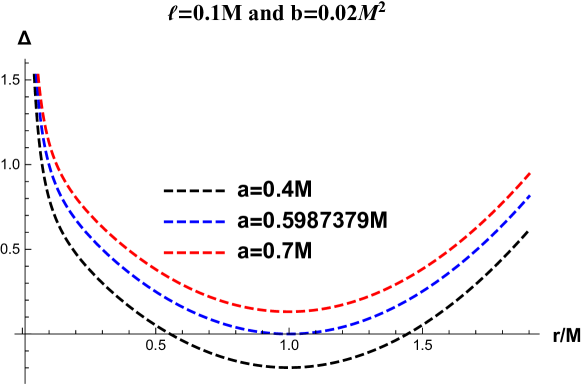
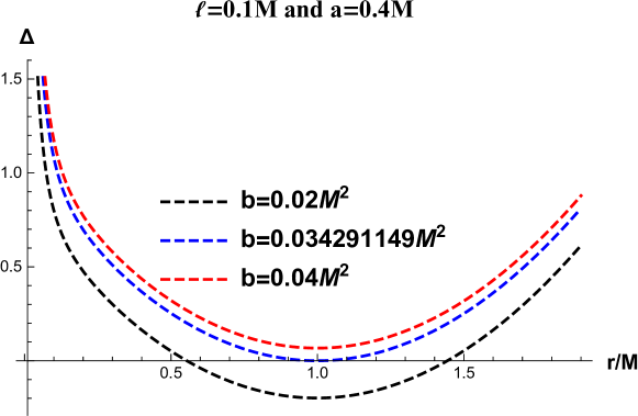
Figure 1: The left one gives the variation of $\Delta$ for various values of $a$ with $b=0.02M^{2}$ and $\ell=0.1M$, and the right one gives variation for various values of $b$ with $a=0.4M$ and $\ell=0.1M$.

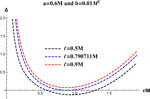
Figure 2: It gives variation of $\Delta$for various values of $\ell$ with $b=0.01M^{2}$ and $a=0.6M$.

The plots in Figs. (1, 2) show some critical values of the parameter involved in the metric. We observe that there exists critical values of $a$, for fixed values of $b$ and $\ell$. Similarly, we get critical values of $b$ for fixed values of $a$ and $\ell$ as well as critical values of $\ell$ for fixed values of $b$ and $a$. The critical values of $a$, $b$, and $\ell$ are designated by $a_{c},b_{c}$, and $\ell_{c}$ respectively. In these cases, $\Delta=0$ has only one root. For $a<a_{c}$ we have black hole, however, for $a>a_{c}$ we have naked singularity. Similarly for $b<b_{c}$ we have black hole, but for $b>b_{c}$ we have naked singularity, and for $\ell<\ell_{c}$ signifies the existence of black hole, whereas $\ell>\ell_{c}$ represents the naked singularity. Numerical computation shows that we have $a_{c}=0.5987379M$ for $b=0.02M^{2}$ and $\ell=0.1M$. Similarly, for $a=0.4M$ and $\ell=0.1M$ we have $b_{c}=0.034291149M^{2}$ and for $a=0.6M$ and $b=0.01M^{2}$ we find $\ell_{c}=0.790711M$. We now focus on the static limit surface (SLS). On the SLS, the asymptotic time-translational Killing vector becomes null which is mathematically written down as

$$g_{tt}=\rho^{2}-2M_{b}r=0.$$ (6)

The real positive solutions of the above equation give radial coordinates of the ergosphere.

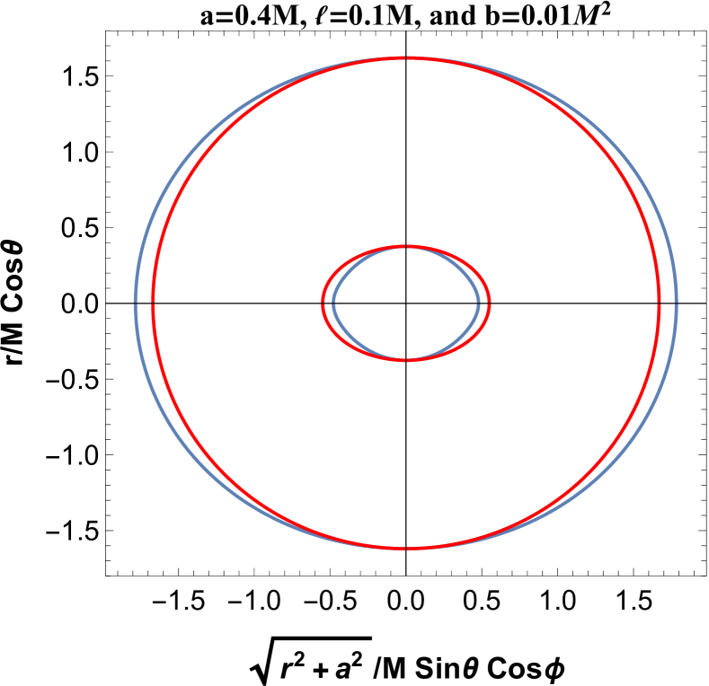
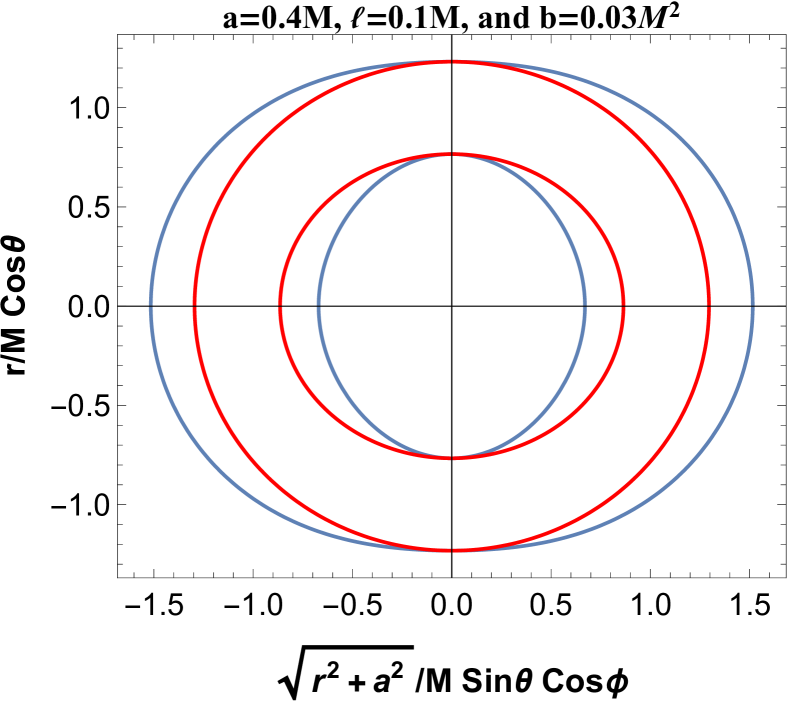
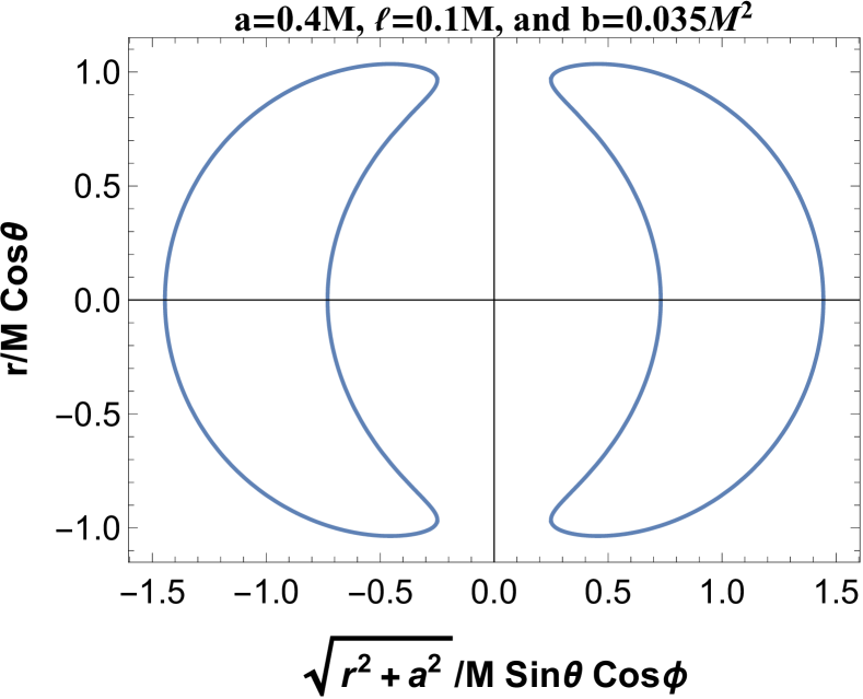
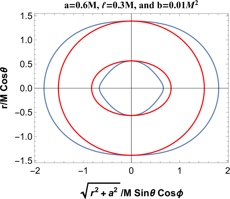
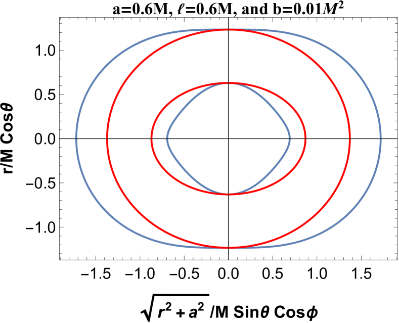
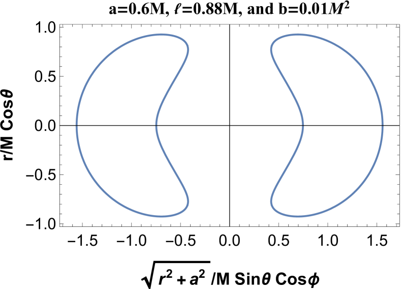
Figure 3: The cross-section of the event horizon (outer red line), SLS (outer blue dotted line), and ergoregion of non-commutative Kerr-like black holes.

The ergosphere, which lies between SLS and the event horizon, is depicted above. As we have learned in the paper PENROSE , energy can be extracted from the ergosphere in this situation indeed. It reveals that the shape and size of the ergosphere depend on the rotational parameter $a$, the non-commutative parameter $b$, and the parameter $\ell$. The size of the ergosphere increases with the increase in the value of parameters $b$ and $\ell$.

IV Superradiance scattering of the scalar field off rotating Simpson-Visser black hole augmented with non-commutative correction

To study the superradiance scattering of a scalar field $\Phi$ off a non-commutative Simpson-Visser black hole field we consider the Klein-Gordon equation corresponding to this curved spacetime. It is given by

$$\left(\bigtriangledown_{\alpha}\bigtriangledown^{\alpha}+\mu^{2}\right)\Phi(t,r,\theta,\phi)=\left[\frac{-1}{\sqrt{-g}}\partial_{\sigma}\left(g^{\sigma\tau}\sqrt{-g}\partial_{\tau}\right)+\mu^{2}\right]\Phi(t,r,\theta,\phi) = 0,$$ (7)

which is a second-order coupled differential equation. Here $\mu$ represents the mass of the scalar field $\Phi$. To separate this coupled differential equation into radial and angular parts we now use the standard separation of variables method for the equation Eq.(7). The following ansatz in the Boyer-Lindquist coordinates $(t,r,\theta,\phi)$

$$\Phi(t,r,\theta,\phi)=F_{\omega jm}(r)\Theta(\theta)e^{-i\omega t}e^{im\phi},\quad j\geq 0,\quad-j\leq m\leq j,\quad\omega>0,$$ (8)

is found to be useful to get the required decoupled equations. Here $R_{\omega jm}(r)$ represents the radial function and $\Theta(\theta)$ refers to the oblate spheroidal wave function. The symbols $j$, $m$, and $\omega$, respectively, stand for the angular eigenfunction, angular quantum number, and the positive frequency of the field under investigation as viewed by a far away observer. The use of the suitable ansatz (8) enables us to separate the differential equation (7) into the following two ordinary second-order differential equations. The radial part of the equation reads

$$\frac{d}{dr}(\Delta\frac{dF_{\omega jm}(r)}{dr})+(\frac{((r^{2}+a^{2}+\ell^{2})\omega-am)^{2}}{\Delta})F_{\omega lm}(r)$$

$$-(\mu^{2}r^{2}+\mu^{2}\ell^{2}+j(j+1)+a^{2}\omega^{2}-2m\omega a)F_{\omega lm}(r)=0,$$ (9)

and the angular part of this is

$$\sin\theta\frac{d}{d\theta}\left(\sin\theta\frac{d\Theta_{\omega jm}(\theta)}{d\theta}\right)+\left(j(j+1)\sin^{2}\theta-\left(\left(a\omega\sin^{2}\theta-m\right)^{2}\right)\right)\Theta_{\omega jm}(\theta)$$

$$+a^{2}\mu^{2}\sin^{2}\theta\cos^{2}\theta~{}\Theta_{\omega jm}(\theta)=0.$$ (10)

We may have a general solution of the radial equation (9) from the knowledge gained from the earlier investigation BEZERRA ; KRANIOTIS , which we do not require here since we are intended in studying the scattering of the field $\Phi$ keeping in view the superradiance phenomena with prime importance. We will use the conventional asymptotic matching procedure which has been found useful for this type of study STRO1 ; STRO2 ; TEUK ; PAGE ; RAN . The rationale adopted in the important contributions STRO1 ; STRO2 ; TEUK ; PAGE ; MK ; RAN led us to reach the required result without going through the general solution of the equation (9). The radial part of the equation (9) is taken into account to find an asymptotic solution. We invite Regge-Wheeler-like coordinate $r_{*}$ which is defined below.

$$r_{*}\equiv\int dr\frac{r^{2}+a^{2}+\ell^{2}}{\Delta},\quad\left(r_{*}\rightarrow-\infty\quad\text{at event horizon},\quad r_{*}\rightarrow\infty\quad\text{at infinity}\right).$$ (11)

Our requirement demands this very choice of co-ordinate as it is beneficial to deal with the radial equation in this situation.

A new radial function $\mathcal{F}_{\omega jm}\left(r_{*}\right)=\sqrt{r^{2}+a^{2}+\ell^{2}}F_{\omega jm}(r)$ is introduced at this stage and after going through a few steps of algebra we obtain the following radial equation in the desired shape

$$\frac{d^{2}\mathcal{F}_{\omega lm}\left(r_{*}\right)}{dr_{*}^{2}}+V_{\omega jm}(r)\mathcal{F}_{\omega jm}\left(r_{*}\right)=0.$$ (12)

Note that an effective potential comes into the picture which has a crucial role in the scattering of the scalar field $\Phi$. The effective potential reads

$$V_{\omega jm}(r) = \left(\omega-\frac{ma}{r^{2}+a^{2}+\ell^{2}}\right)^{2}-\frac{\Delta}{\left(r^{2}+a^{2}+\ell^{2}\right)^{2}}\left[\right.j(j+1)+a^{2}\omega^{2}-2ma\omega+\mu^{2}r^{2}$$

$$\left.+\mu^{2}\ell^{2}+\sqrt{r^{2}+a^{2}+\ell^{2}}\frac{d}{dr}\left(\frac{r\Delta}{\left(r^{2}+a^{2}+\ell^{2}\right)^{\frac{3}{2}}}\right)\right],$$

It turns out that this problem is comparable to the scattering of the scalar field $\Phi$ under the effective potential (IV). Let us now see the asymptotic behavior of the scattering potential at the event horizon and spatial infinity. We find that the potential in the asymptotic limit at the event horizon acquires the following simplified form

$$\lim_{r\rightarrow r_{eh}}V_{\omega jm}(r)=\left(\omega-m\Omega_{eh}\right)^{2}\equiv k_{eh}^{2},$$ (14)

and after a few steps of algebra, the potential turns into the following at spatial infinity.

$$\lim_{r\rightarrow\infty}V_{\omega jm}(r)=\omega^{2}\lim_{r\rightarrow\infty}\frac{\mu^{2}r^{2}\Delta}{(r^{2}+a^{2}+\ell^{2})^{2}}=\omega^{2}-\mu^{2}\equiv k^{2}_{\infty}.$$ (15)

Here $\Omega_{eh}=\frac{a}{r_{eh}^{2}+\ell^{2}+a^{2}}$. Although the potential shows constant behavior at the two extremal points namely at the event horizon and at spatial infinity, the numerical values of the constants are different indeed at the two extremal points.

After scrutinizing the behavior of the potential at the two extreme points, we now make the way to explore the asymptotic behavior of the radial solution. After a little algebra, we find that in the asymptotic limit the radial equation (12) has the solution

$$F_{\omega jm}(r)\rightarrow\left\{\begin{array}[]{cl}\frac{\mathcal{E}_{in}^{eh}e^{-ik_{eh}r_{*}}}{\sqrt{r_{eh}^{2}+a^{2}+\ell^{2}}}&\text{ for }r\rightarrow r_{eh}\\ \mathcal{E}_{in}^{\infty}\frac{e^{-ik_{\infty}r_{*}}}{r}+\mathcal{E}_{ref}^{\infty}\frac{e^{ik_{\infty}r_{*}}}{r}&\text{ for }r\rightarrow\infty,\end{array}\right\}$$ (16)

where $\mathcal{D}_{in}^{eh}$ is representing the amplitude of the incoming scalar wave at event horizon($r_{eh}$) and $\mathcal{D}_{in}^{\infty}$ stands for the amplitude of that incoming scalar wave at infinity $(\infty)$. At spatial infinity, the amplitude of the reflected part of the scalar wave is designated by $\mathcal{D}_{ref}^{\infty}$. We will now be able to compute the Wronskian which in turn will lead us to calculate its limiting values for the region adjacent to the event horizon and at infinity. The Wronskian for the event horizon has the expression

$$W_{eh}=\left(F_{\omega jm}^{eh}\frac{dF_{\omega jm}^{*eh}}{dr_{*}}-F_{\omega jm}^{*eh}\frac{dF_{\omega jm}^{eh}}{dr_{*}}\right),$$ (17)

and the Wronskian at infinity is given by the expression

$$W_{\infty}=\left(F_{\omega jm}^{\infty}\frac{dF_{\omega jm}^{*\infty}}{dr_{*}}-F_{\omega jm}^{*\infty}\frac{dF_{\omega jm}^{\infty}}{dr_{*}}\right).$$ (18)

Note that the solutions are linearly independent. Therefore, the information concerning the standard theory of ordinary differential equations leads us to draw an inference that the Wronskian associated with the solutions will be independent of $r^{*}$. On that account, the Wronskian evaluated at the horizon is compatible to equate with the Wronskian evaluated at infinity. It is in fact associated with the flux conservation of the process REVIEW in the physical sense. A fascinating relation between the amplitudes of incoming and reflected waves at different regions of interest results from equating the Wronskian. The said relation reads

$$\left|\mathcal{E}_{ref}^{\infty}\right|^{2}=\left|\mathcal{E}_{in}^{\infty}\right|^{2}-\frac{k_{eh}}{k_{\infty}}\left|\mathcal{E}_{in}^{eh}\right|^{2}.$$ (19)

Note that if $\frac{k_{eh}}{k_{\infty}}<0$, i.e. $\omega<m\Omega_{eh}$, the scalar wave will be superradiantly amplified, since the relation $\left|\mathcal{E}_{ref}^{\infty}\right|^{2}>\left|\mathcal{E}_{in}^{\infty}\right|^{2}$ precisely holds in this situation.

IV.1 Amplification factor $Z_{jm}$ for superradiance

The radial equation (9) which we have obtained can be express in the following form after a few steps of algebra

$$\Delta^{2}\frac{d^{2}F_{\omega jm}(r)}{dr^{2}}+\Delta\frac{d\Delta}{dr}\cdot\frac{dF_{\omega jm}(r)}{dr}$$

$$+\left(\left(\left(r^{2}+a^{2}+\ell^{2}\right)\omega-am\right)^{2}-\Delta\left(\mu^{2}r^{2}+\mu^{2}\ell^{2}+j(j+1)+a^{2}\omega^{2}-2ma\omega\right)\right)F_{\omega jm}(r)=0.$$ (20)

Our next step is to find out the solution for the near and the far region and in turn make an attempt to have a single solution by matching the solution for near-region at infinity with the solution for the far-region at its initial point such that this particular solution be amenable in the vicinity of the cardinal region. At this stage, it is convenient to make use of a new variable $y$ which is defined by $u=\frac{r-r_{eh}}{r_{eh}-r_{ch}}$. In terms of $y$ the equation (20) can be written down as

$$u^{2}(u+1)^{2}\frac{\mathrm{d}^{2}F_{\omega jm}(u)}{\mathrm{d}u^{2}}+u(u+1)(2u+1)\frac{\mathrm{d}F_{\omega jm}(y)}{\mathrm{d}u}$$ (21)

$$+\left(\mathcal{Q}^{2}u^{4}+B^{2}-j(j+1)u(u+1)-\frac{\mu^{2}\mathcal{Q}^{2}}{\omega^{2}}u^{3}(u+1)-\mu^{2}r_{eh}^{2}u(u+1)-\frac{2\mu^{2}r_{eh}\mathcal{Q}}{\omega}u^{2}(u+1)\right)F_{\omega jm}(y)=0,$$

with the approximation $a\omega\ll 1$. In equation (IV.1, the $B$ and $B\mathcal{Q}$ have the following expressions:

$$B = \frac{(\omega-m\Omega_{eh}}{r_{eh}-r_{ch}}r_{eh}^{2}$$

$$\mathcal{Q} = \left(r_{eh}-r_{ch}\right)\omega.$$ (22)

Let us now focus on the near-region solution where we have $\mathcal{Q}y\ll 1$ and $\mu^{2}r_{eh}^{2}\ll 1$. Therefore, for the near-region the above equation gets a simplified form:

$$u^{2}(u+1)^{2}\frac{\mathrm{d}^{2}F_{\omega jm}(y)}{\mathrm{d}u^{2}}+u(u+1)(2u+1)\frac{\mathrm{d}F_{\omega jm}(u)}{\mathrm{d}u}+\left(B^{2}-j(j+1)u(u+1)\right)F_{\omega jm}(r)=0.$$ (23)

Since the Compton wavelength of the boson participating in the scattering process is much smaller than the size of the black hole the approximation $\left(\mu^{2}r_{eh}^{2}\ll 1\right)$ is regarded in the process. So, the general solution of the above equation in terms of associated Legendre function of the first kind $P_{\lambda}^{\nu}(y)$ can be expressed as

$$F_{\omega jm}(u)=dP^{2iB}_{\frac{\sqrt{1+4j(j+1)}-1}{2}}(1+2u).$$ (24)

Now, we use the relation

$$P_{\lambda}^{\nu}(z)=\frac{1}{\Gamma(1-\nu)}\left(\frac{1+z}{1-z}\right)^{\nu/2}{}_{2}F_{1}\left(-\lambda,\lambda+1;1-\nu;\frac{1-z}{2}\right),$$ (25)

that facilitates us to express $F_{\omega jm}(y)$ in terms of the ordinary hypergeometric functions ${}_{2}F_{1}(a,b;c;z)$ :

$$F_{\omega jm}(u)=d\left(\frac{u}{u+1}\right)^{-iB}{}_{2}F_{1}\left(\frac{1-\sqrt{1+4j(j+1)}}{2},\frac{1+\sqrt{1+4j(j+1)}}{2};1-2iB;-u\right).$$ (26)

We have mentioned already that we are intended to design a single solution using the matching condition at the desired (cardinal) position where the two solutions mingle with each other. Therefore, we need to have the behavior of the above expression (26) for large $u$. For large u, i.e. $(u\to\infty$) the Eq.(26) turns into

$$F_{\text{near-large }u}\sim d \left(\frac{\Gamma(\sqrt{1+4j(j+1)})\Gamma(1-2iB)}{\Gamma\left(\frac{1+\sqrt{1+4j(j+1)}}{2}-2iB\right)\Gamma\left(\frac{1+\sqrt{1+4j(j+1)}}{2}\right)}u^{\frac{\sqrt{1+4j(j+1)}-1}{2}}+\right.$$ (28)

$$\frac{\Gamma(-\sqrt{1+4j(j+1)})\Gamma(1-2iB)}{\Gamma\left(\frac{1-\sqrt{1+4j(j+1)}}{2}\right)\Gamma\left(\frac{1-\sqrt{1+4j(j+1)}}{2}-2iB\right)}u^{\left.-\frac{\sqrt{1+4j(j+1)}+1}{2}\right)}.$$

Let us look at the solution for the far region. To match the solution of far and near regions at the cardinal region the behavior of solution (20) with the approximations $u+1\approx u$ and $\mu^{2}r_{eh}^{2}\ll 1$ is to be computed. We may drop all the terms except those which describe the free motion with momentum $j$ and after the dropping out of all these terms the equation (20) reduces to

$$\frac{\mathrm{d}^{2}F_{\omega jm}(u)}{\mathrm{d}u^{2}}+\frac{2}{u}\frac{\mathrm{d}F_{\omega jm}(u)}{\mathrm{d}u}+\left(k_{l}^{2}-\frac{j(j+1)}{u^{2}}\right)F_{\omega jm}(u)=0,$$ (29)

where $k_{l}\equiv\frac{\mathcal{Q}}{\omega}\sqrt{\omega^{2}-\mu^{2}}$. Note that the equation (29) can be solved exactly and the most general solution of the equation (29) is

$$F_{\omega jm,\text{ far }}=e^{-iky}(f_{1}u^{\frac{\sqrt{1+4j(j+1)}-1}{2}}M(\frac{1+\sqrt{1+4j(j+1)}}{2},1+\sqrt{1+4j(j+1)},2ik_{l}u)+$$ (30)

$$f_{2}u^{-\frac{\sqrt{1+4j(j+1)}+1}{2}}M(\frac{1-\sqrt{1+4j(j+1)}}{2},1-\sqrt{1+4j(j+1)},2ik_{l}u)),$$

where $M(a;b;y)$ is representing the confluent hypergeometric Kummer function of the first kind. In order to equate the solution (IV.1) with the far-region limiting solution of (26) standing in Eq. (28), we look for the small $y$ behavior of the solution (IV.1). See that the equation (IV.1) turns into

$$F_{\omega jm,\text{ far-small }\mathrm{u}}\sim u^{-\frac{1+\sqrt{1+4j(j+1)}}{2}},$$ (31)

for small u, i.e. $(u\to 0)$. The solution (28) and (31) are susceptible to match, since these two have a common mingling region. The matching of the asymptotic solutions (28) and (31) facilitates us to compute the scalar wave flux at infinity which reads

$$f_{1}= d\frac{\Gamma(\sqrt{1+4j(j+1)})\Gamma(1-2iB)}{\Gamma\left(\frac{1+\sqrt{1+4j(j+1)}}{2}-2iB\right)\Gamma\left(\frac{1+\sqrt{1+4j(j+1)}}{2}\right)},$$ (32)

$$f_{2}= d\frac{\Gamma(-\sqrt{1+4j(j+1)})\Gamma(1-2iB)}{\Gamma\left(\frac{1-\sqrt{1+4j(j+1)}}{2}-2iB\right)\Gamma\left(\frac{1-\sqrt{1+4j(j+1)}}{2}\right)}.$$

If we expand equation (IV.1) around infinity it results

$$f_{1}\frac{\Gamma(1+\sqrt{1+4j(j+1)})}{\Gamma\left(\frac{1+\sqrt{1+4j(j+1)}}{2}\right)}k_{l}^{-\frac{1+\sqrt{1+4j(j+1)}}{2}}\left((-2i)^{-\frac{1+\sqrt{1+4j(j+1)}}{2}}\frac{e^{-ik_{l}u}}{u}+(2i)^{-\frac{1+\sqrt{1+4j(j+1)}}{2}}\frac{e^{ik_{l}u}}{u}\right)+$$ (33)

$$f_{2}\frac{\Gamma(1-\sqrt{1+4j(j+1)})}{\Gamma\left(\frac{1-\sqrt{1+4j(j+1)}}{2}\right)}k_{l}^{\frac{\sqrt{1+4j(j+1)}-1}{2}}\left((-2i)^{\frac{\sqrt{1+4j(j+1)}-1}{2}}\frac{e^{-ik_{l}u}}{u}+(2i)^{\frac{\sqrt{1+4j(j+1)}-1}{2}}\frac{e^{ik_{l}u}}{u}\right),$$

if the approximations $\frac{1}{u}\sim\frac{\mathcal{Q}}{\omega}\cdot\frac{1}{r},\quad e^{\pm ik_{l}u}\sim e^{\pm i\sqrt{(\omega^{2}-\mu^{2})}r}$ are made functional. If a comparison of Eq. (IV.1) is made with the radial solution (16) we have

$$F_{\infty}(r)\sim\mathcal{E}_{in}^{\infty}\frac{e^{-i\sqrt{\omega^{2}-\mu^{2}}r^{*}}}{r}+\mathcal{E}_{ref}^{\infty}\frac{e^{i\sqrt{\omega^{2}-\mu^{2}}r^{*}}}{r},\quad\text{ for }\quad r\rightarrow\infty,$$

where

$$\begin{array}[]{c}\mathcal{E}_{in}^{\infty}=\frac{\mathcal{Q}}{\omega}\left(f_{1}(-2i)^{-\frac{1+\sqrt{1+4j(j+1)}}{2}}\frac{\Gamma(1+\sqrt{1+4j(j+1)})}{\Gamma\left(\frac{1+\sqrt{1+4j(j+1)}}{2}\right)}k_{l}^{-\frac{1+\sqrt{1+4j(j+1)}}{2}}+\right.\\ \left.f_{2}(-2i)^{\frac{\sqrt{1+4j(j+1)}-1}{2}}\frac{\Gamma(1-\sqrt{1+4j(j+1)})}{\Gamma\left(\frac{1-\sqrt{1+4j(j+1)}}{2}\right)}k_{l}^{\frac{\sqrt{1+4j(j+1)}-1}{2}}\right),\end{array}$$

and

$$\begin{array}[]{l}\mathcal{E}_{ref}^{\infty}=\frac{\mathcal{Q}}{\omega}\left(f_{1}(2i)^{-\frac{1+\sqrt{1+4j(j+1)}}{2}}\frac{\Gamma(1+\sqrt{1+4j(j+1)})}{\Gamma\left(\frac{1+\sqrt{1+4j(j+1)}}{2}\right)}k_{l}^{-\frac{1+\sqrt{1+4j(j+1)}}{2}}+\right.\\ \left.f_{2}(2i)\frac{\sqrt{1+4j(j+1)}-1}{2}\frac{\Gamma(1-\sqrt{1+4j(j+1)})}{\Gamma\left(\frac{1-\sqrt{1+4j(j+1)}}{2}\right)}k_{l}^{\frac{\sqrt{1+4j(j+1)}-1}{2}}\right).\end{array}$$

Substituting the expressions of $f_{1}$ and $f_{2}$ from Eq. (IV.1) into the above expressions, we land onto

$$\mathcal{E}_{in}^{\infty} = \frac{d(-2i)^{-\frac{1+\sqrt{1+4j(j+1)}}{2}}}{\sqrt{(\omega^{2}-\mu^{2})}}\cdot\frac{\Gamma(\sqrt{1+4j(j+1)})\Gamma(1+\sqrt{1+4j(j+1)})}{\Gamma\left(\frac{1+\sqrt{1+4j(j+1)}}{2}-2iB\right)\left(\Gamma\left(\frac{1+\sqrt{1+4j(j+1)}}{2}\right)\right)^{2}}\times$$

$$\Gamma(1-2iB)k_{l}^{\frac{1-\sqrt{1+4j(j+1)}}{2}}+\frac{d(-2i)^{\frac{\sqrt{1+4j(j+1)}-1}{2}}}{\sqrt{(\omega^{2}-\hat{\mu}^{2})}}\times$$

$$\frac{\Gamma(1-\sqrt{1+4j(j+1)})\Gamma(-\sqrt{1+4j(j+1)})}{\left(\Gamma\left(\frac{1-\sqrt{1+4j(j+1)}}{2}\right)\right)^{2}\Gamma\left(\frac{1-\sqrt{1+4j(j+1)}}{2}-2iB\right)}\Gamma(1-2iB)k_{l}^{\frac{1+\sqrt{1+4j(j+1)}}{2}},$$

and

$$\mathcal{E}_{ref}^{\infty} = \frac{d(2i)^{-\frac{1+\sqrt{1+4j(j+1)}}{2}}}{\sqrt{(\omega^{2}-\mu^{2})}}\cdot\frac{\Gamma(\sqrt{1+4j(j+1)})\Gamma(1+\sqrt{1+4j(j+1)})}{\Gamma\left(\frac{1+\sqrt{1+4j(j+1)}}{2}-2iB\right)\left(\Gamma\left(\frac{1+\sqrt{1+4j(j+1)}}{2}\right)\right)^{2}}\times$$

$$\Gamma(1-2iB)k_{l}^{\frac{1-\sqrt{1+4j(j+1)}}{2}}+\frac{d(2i)^{\frac{\sqrt{1+4j(j+1)}-1}{2}}}{\sqrt{(\omega^{2}-\mu^{2})}}\times$$

$$\frac{\Gamma(1-\sqrt{1+4j(j+1)})\Gamma(-\sqrt{1+4j(j+1)})}{\left(\Gamma\left(\frac{1-\sqrt{1+4j(j+1)}}{2}\right)\right)^{2}\Gamma\left(\frac{1-\sqrt{1+4j(j+1)}}{2}-2iB\right)}\Gamma(1-2iB)k_{l}^{\frac{1+\sqrt{1+4j(j+1)}}{2}}.$$

Ultimately, we reach the expression of the amplification factor that results out to be

$$Z_{jm}\equiv\frac{\left|\mathcal{E}_{ref}^{\infty}\right|^{2}}{\left|\mathcal{E}_{in}^{\infty}\right|^{2}}-1.$$ (36)

Equation (36) is a general expression of the amplification factor obtained by making use of the asymptotic matching method. A striking feature follows if $\frac{\left|\mathcal{E}_{ref}^{\infty}\right|^{2}}{\left|\mathcal{E}_{in}^{\infty}\right|^{2}}$ acquires a value greater than unity. There will be a definite gain in the amplification factor that corresponds to superradiance phenomena. However, a negative value of the amplification factor indicates a dropping down of the amplification that corresponds to the non-occurrence of the superradiance phenomena. In Fig. (6), we have given a graphical presentation of the variation $Z_{jm}$ with $M\omega$. Here the leading multi-poles $j=1$, and $2$ have been taken into consideration. Taking different values of the parameter $\ell$ the plots for the multi-poles $j=1$, and $2$ have been displayed in Fig. (6)

A judicious look on Fig. (4) and Fig. (5), makes it evident that superradiance for a particular value of $j$ occurs when the allowed azimuthal values for $J$, i.e. the values of $m$ are restricted to $m>0$. For negative value $m$, however, the amplification factor takes a negative value which refers to the nonoccurrence of superradiance. It also becomes transparent from Fig. (6) that if the numerical value of the parameter $\ell$ increases the superradiance process gets enhanced and the reverse is the case when the value of the parameter $\ell$ drops down. Fig. (8) shows the effect of the spin parameter $a$ on the superradiance process. Here it is clearly observed that the superradiance process intensifies with an increase in the spin parameter $a$. The quantum effect of gravity which is amended in our model is characterized by non-commutative parameter $b$. Fig. (7) shows that the superradiance scenario decreases with the increase in the value of the non-commutative parameter $b$. Therefore, amendment of the quantum gravity effect makes the superradiance process moderate.

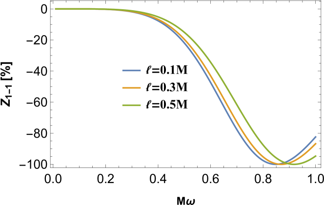
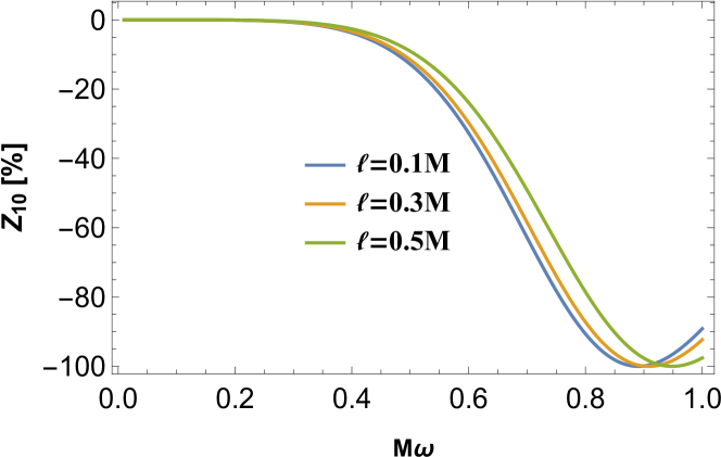
Figure 4: Variation of amplification factors with $\ell$ for non-superradiant multi-poles with $\mu=0.1,b=0.01M^{2}$, and $a=0.52M$.

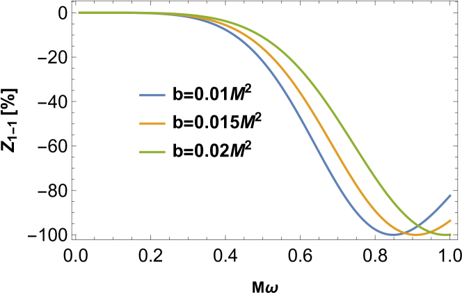
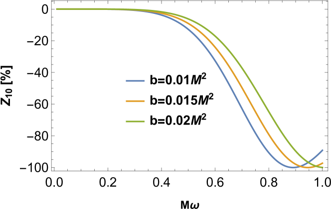
Figure 5: Variation of amplification factors with $b$ for non-superradiant multi-poles with $\mu=0.1,\ell=0.1M$, and $a=0.42M$.

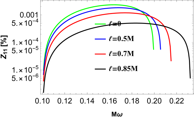
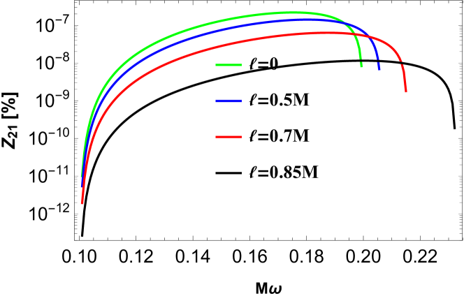
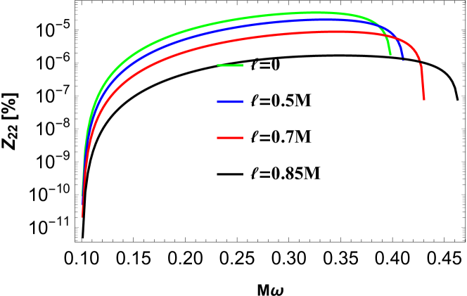
Figure 6: Variation of amplification factors with $\ell$ for various multi-poles with $\mu=0.1,b=0.01M^{2}$, and $a=0.52M$.

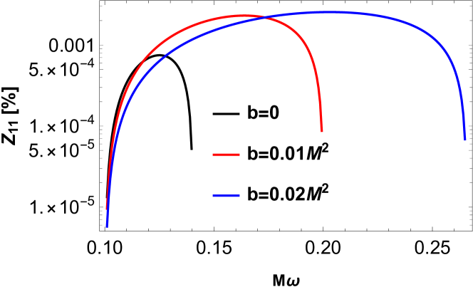
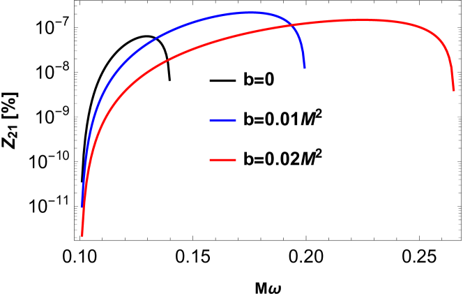
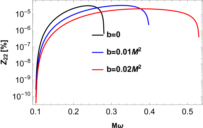
Figure 7: Variation of amplification factors with $b$ for various multi-poles with $\mu=0.1,\ell=0.1M$, and $a=0.52M$.

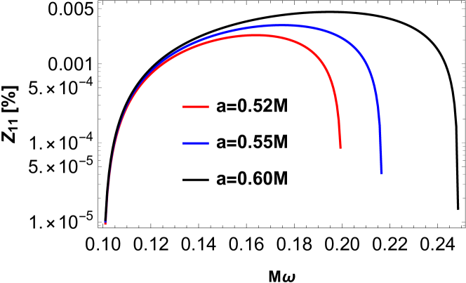
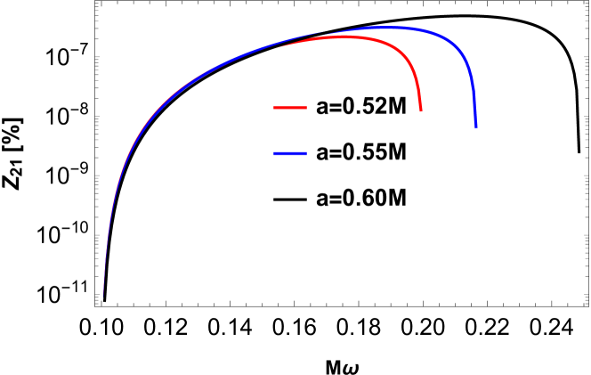
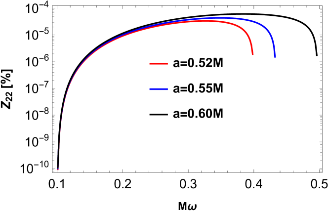
Figure 8: Variation of amplification factors with $a$ for various multi-poles with $\mu=0.1,b=0.01M^{2}$, and $\ell=0.1M$.

IV.2 Superradiant instability for Simpson-Visser black hole in the non-commutative setting

If the superradiant field gets trapped in an enclosed system, then the stability of the background black hole will be disturbed as a result of energy extraction. In this situation, the scalar field interacts with the background black hole repeatedly and the scattered wave amplitude increases exponentially which leads to superradiant instability. The possible occurrence of this type of instability was first reported by Press and Teukolsky and they termed this phenomenon as black hole bomb PRESS ; TEUK . Let us look at (9) and write it as follows

$$\Delta\frac{d}{dr}\left(\Delta\frac{dF_{\omega jm}}{dr}\right)+\mathcal{G}F_{\omega jm}=0,$$ (37)

were $\mathcal{G}$ has the form

$$\mathcal{G}\equiv\left(\left(r^{2}+a^{2}+\ell^{2}\right)\omega-ma\right)^{2}+\Delta\left(2ma\omega-j(j+1)-\mu^{2}r^{2}-\mu^{2}\ell^{2}\right).$$

for a slowly rotating black hole, i.e when $a\omega\ll 1$. So, black hole bomb mechanism will be feasible if we have the following solutions for the radial equation (37)

$$F_{\omega jm}\sim\left\{\begin{array}[]{ll}e^{-i(\omega-m\Omega_{eh})r_{*}}&\text{ as }r\rightarrow r_{eh}\left(r_{*}\rightarrow-\infty\right)\\ \frac{e^{-\sqrt{\mu^{2}-\omega^{2}}r_{*}}}{r}&\text{ as }r\rightarrow\infty\left(r_{*}\rightarrow\infty\right)\end{array}\right.$$

The above solution corresponds to a physical boundary condition that the scalar wave at the black hole horizon is purely in-going while at spatial infinity it is decaying only exponentially, provided the condition $\omega^{2}<\ mu^{2}$ is maintained.

Now, in terms of the new radial function

$$\psi_{\omega jm}\equiv\sqrt{\Delta}F_{\omega jm},$$

the radial equation (37) can be expressed as

$$(\frac{d^{2}r}{dr^{2}}+\omega^{2}-V)\psi_{\omega jm}=0.$$ (38)

with

$$\omega^{2}-V=\frac{\mathcal{G}+\frac{1}{4}\left(-\frac{8\sqrt{b}M\sqrt{\ell^{2}+r^{2}}}{\sqrt{\pi}r^{2}}-\frac{2r\left(M-\frac{4\sqrt{b}M}{\sqrt{\pi}r}\right)}{\sqrt{\ell^{2}+r^{2}}}+2r\right)^{2}}{\Delta^{2}},$$

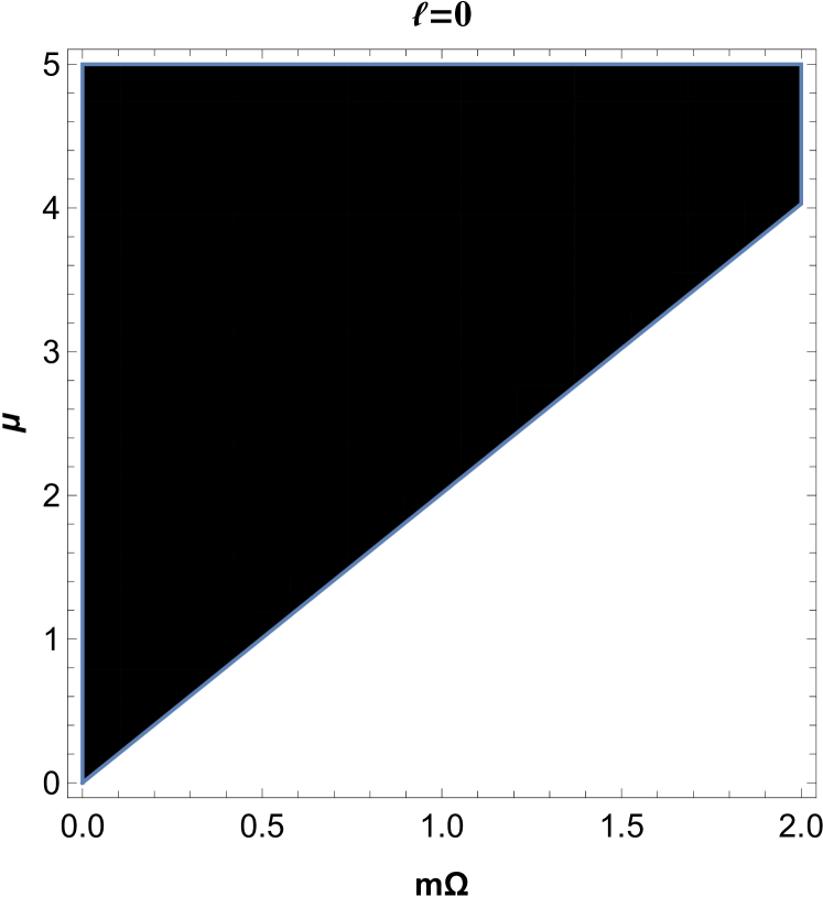
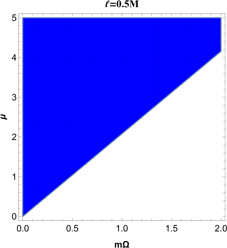
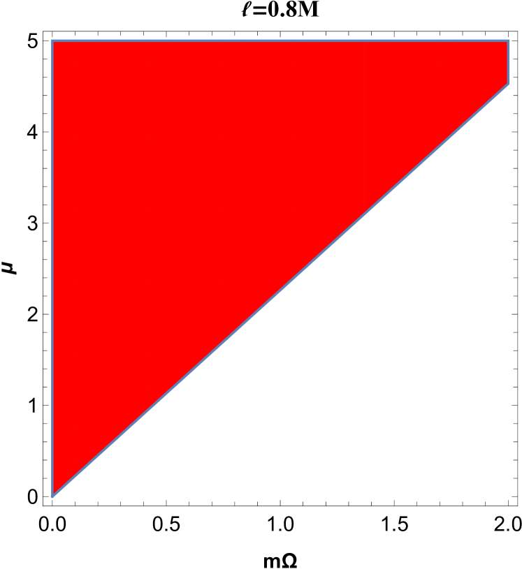
Figure 9: Parameter space($m\Omega$-$\mu$) for massive scalar field where the colored area represents the region with stable dynamics and the non-colored area represents the region with unstable dynamics. Here $a=0.52M\quad\text{and}\quad b=0.01M^{2}$

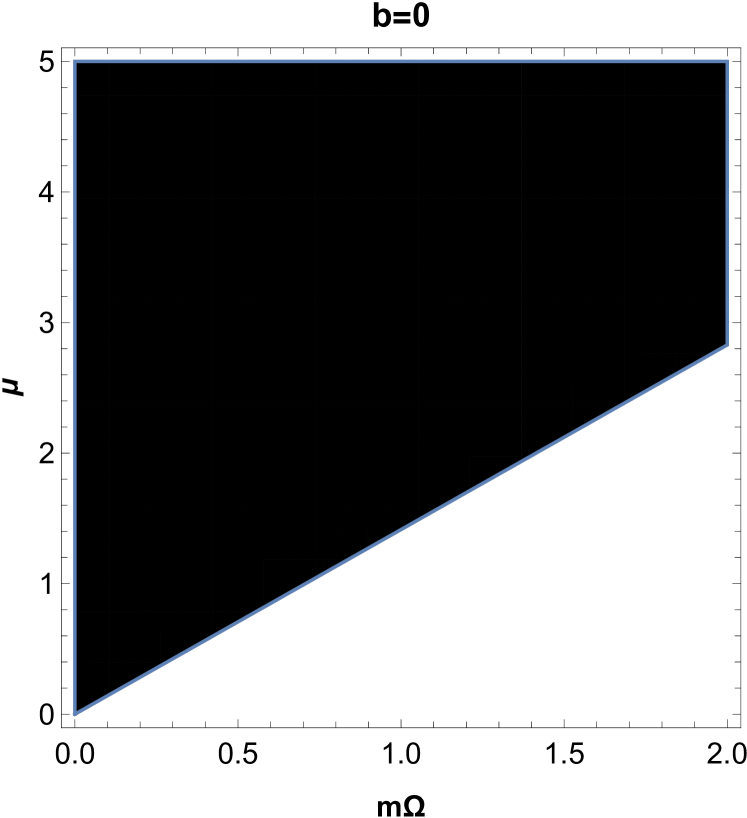
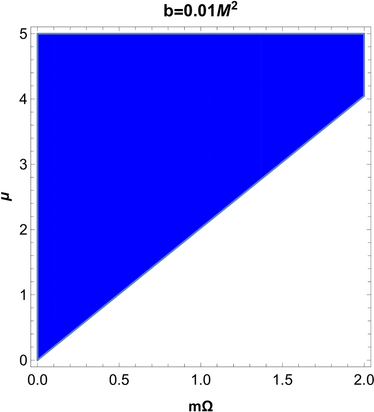
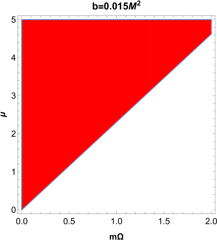
Figure 10: Parameter space($m\Omega$-$\mu$) for massive scalar field where the colored area represents the region with stable dynamics and the non-colored area represents the region with unstable dynamics. Here $a=0.52M\quad\text{and}\quad\ell=0.2M$

It can be identified with the Regge-Wheel equation. If we now discard the terms $\mathcal{O}\left(1/r^{2}\right)$, the effective potential $V(r)$ acquires the following asymptotic form

$$V(r)=\mu^{2}-\frac{4M\omega^{2}}{r}+\frac{2M\mu^{2}}{r}.$$ (39)

The potential (39) will be able to support the trapping of superradiant waves conspicuously if its asymptotic derivative becomes positive: $V^{\prime}\rightarrow 0^{+}$ for large $r$, i.e. when $r\rightarrow\infty$ HOD . This together with the condition of occurrence of superradiance amplification of scattered waves $\omega<m\Omega_{eh}$, we can mark a specified regime where $\frac{\mu}{\sqrt{2}}<\omega^{2}<m\Omega_{eh}$. In this regime, the massive scalar field in the modified Simpson-Visser background may experience superradiant instability. This indeed corresponds to the black hole bomb phenomena. However, the dynamics of the massive scalar field in the extended Simpson-Visser background will remain stable when $\mu\geq\sqrt{2}m\Omega_{eh}$

V Photon orbit and black hole shadow

This section is devoted to the study of the black hole shadow associated with this modified model where the non-commutative character of spacetime has been amended in the standard Simpson-Visser background. From the illuminating studies related to the black hole shadow from which we have got the road map for the investigation concerning the shadow SDO1 ; SDO2 ; SDO3 ; SDO4 , we bring into our consideration two conserved parameters $\xi$ and $\eta$ as usual to study the shadow. These two are defined by

$$\xi=\frac{L_{z}}{E}\quad\textrm{and}\quad\eta=\frac{\mathcal{Q}}{E^{2}},$$ (40)

where $E,L_{z}$, and $\mathcal{Q}$ refers to the energy, the axial component of the angular momentum, and the Carter constant respectively. In terms of $\xi$ we then express the null geodesics in the Simpson-Visser rotating black hole spacetime:

$$\Sigma\frac{dr}{d\lambda}=\pm\sqrt{R},\quad\Sigma^{2}\frac{d\theta}{d\lambda}=\pm\sqrt{\Theta},$$

$$\Delta\Sigma\frac{dt}{d\lambda}=A-2\operatorname{M\sqrt{r^{2}+\ell^{2}}a\xi},$$

$$\Delta\Sigma\frac{d\phi}{d\lambda}=2M\sqrt{r^{2}+\ell^{2}}a+\frac{\xi}{\sin^{2}\theta}\left(\rho^{2}-2M\sqrt{r^{2}+\ell^{2}}\right),$$ (41)

where $\lambda$ is the affine parameter and $R(r)$ has the expression

$$R(r)=\left[r^{2}+\ell^{2}+a^{2}-a\xi\right]^{2}-\Delta\left[\eta+(\xi-a)^{2}\right],\quad\Theta(\theta)=\eta+a^{2}\cos^{2}\theta-\xi^{2}\cot^{2}\theta.$$ (42)

Now, the radial equation of motion can be written down in the familiar form:

$$\left(\Sigma\frac{dr}{d\lambda}\right)^{2}+V_{eff}=0.$$ (43)

The effective potential $V_{eff}$ in Eq. (43) has the expression

$$V_{eff}=-\left[r^{2}+\ell^{2}+a^{2}-a\xi\right]^{2}+\Delta\left[\eta+(\xi-a)^{2}\right].$$ (44)

The unstable spherical orbit on the equatorial plane, $\theta=\frac{\pi}{2}$ is described by the equation

$$R(r)=0,\quad\frac{dR}{dr}=0,$$ (45)

with conditions $\frac{d^{2}R}{dr^{2}}<0,\quad\textrm{and}\quad\eta=0$.

For more generic orbits $\theta\neq\pi/2$, and $\eta\neq 0$, the solution of Eqn. (45)$r=r_{s}$ gives the $r-$ constant orbit, which is also called spherical orbit, and the conserved parameters of the spherical orbits read

$$\xi_{s} = \frac{\left(a^{2}+\ell^{2}+r^{2}\right)\Delta^{{}^{\prime}}(r)-4\sqrt{r^{2}+\ell^{2}}\Delta(r)}{a\Delta^{{}^{\prime}}(r)},$$ (46)

$$\eta_{s} = \frac{\left(8r\Delta(r)\left(2a^{2}r+(r^{2}+\ell^{2})\Delta^{{}^{\prime}}(r)\right)-(r^{2}+\ell^{2})^{2}\Delta^{{}^{\prime}}(r)^{2}-16r^{2}\Delta(r)^{2}\right)}{a^{2}\Delta^{{}^{\prime}}(r)^{2}},$$

where upper prime stands for differentiation with respect to radial coordinate. The above expressions reduce to the corresponding items for Kerr black hole when both $\ell$ and $b$ approach a vanishing value. It is helpful at this stage to launch two celestial coordinates for studying the shadow in a preferred manner. The celestial coordinates, which are used here to characterize the shadow which would be expected to be viewed by an observer in the sky, could be given by

$$\alpha(\xi,\eta;\theta) = \lim_{r\rightarrow\infty}\frac{-rp^{(\varphi)}}{p^{(t)}}=-\xi_{s}\csc\theta,$$

$$\beta(\xi,\eta;\theta) = \lim_{r\rightarrow\infty}\frac{rp^{(\theta)}}{p^{(t)}}=\sqrt{\left(\eta_{s}+a^{2}\cos^{2}\theta-\xi_{s}^{2}\cot^{2}\theta\right)},$$

where $\left(p^{(t)},p^{(r)},p^{(\theta)},p^{(\phi)}\right)$ are the tetrad components of the momentum of the photon with respect to a locally non-rotating reference frame BARDEEN . With these inputs, the stage is now set for sketching the shadows of this black hole for various cases which are portrayed in the following Figs. (11, 12).

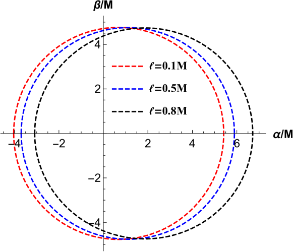
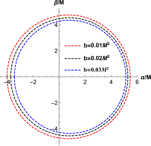
Figure 11: The left panel gives shapes of the shadow for various values of $\ell$ with $a=0.3M$, $b=0.01M^{2}$, and $\theta=\pi/2$. The right panel gives shapes of the shadow for various values of $b$ with $a=0.3M$ , $\ell=0.2M$, and $\theta=\pi/2$.

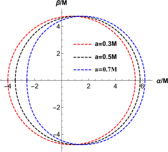
Figure 12: The shapes of the shadow for various values of $a$ with $b=0.01M^{2}$, $\ell=0.2M$, and $\theta=\pi/2$.

A careful look at the plots reveals that the geometrical size of the shadow decreases with an increase in the value of $b$. Furthermore, one can also observe that the left side of the shadow gets shifted towards the right if $\ell$ or $a$ increases.

Let us now introduce the parameters defined by Hioki and Maeda KH to analyze the deviation from the circularity $\left(\delta_{s}\right)$ and the size $\left(R_{s}\right)$ of the shadow cast by the black hole.

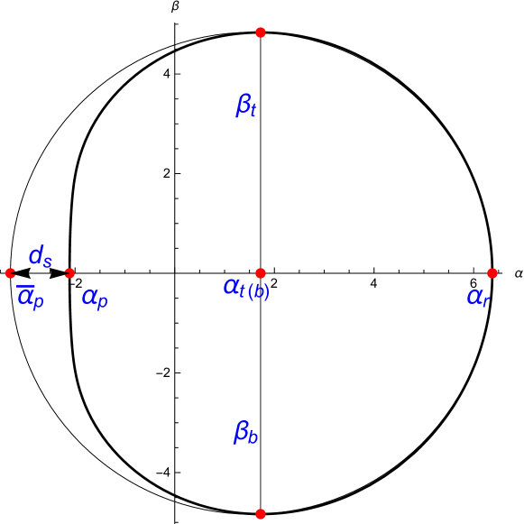
Figure 13: The black hole shadow and reference circle. $ds$ is the distance between the left points of the shadow and the reference circle.

To compute these parameters, we consider five reference points $\left(\alpha_{t},\beta_{t}\right),\left(\alpha_{b},\beta_{b}\right),\left(\alpha_{r},0\right)$ $\left(\alpha_{p},0\right)$ and $\left(\bar{\alpha}_{p},0\right)$. Out of these five points, the first four are describing the top, bottom, rightmost, and leftmost points of the shadow respectively, and the last one refers to the leftmost point of the reference circle in Fig. (13). Therefore, from the geometry we can write

$$R_{s}=\frac{\left(\alpha_{t}-\alpha_{r}\right)^{2}+\beta_{t}^{2}}{2\left|\alpha_{t}-\alpha_{r}\right|}$$

and

$$\delta_{s}=\frac{\left|\bar{\alpha}_{p}-\alpha_{p}\right|}{R_{s}}.$$

In the following Figs. (14, 15, 16, 17) we plot $R_{s}$ and $\delta_{s}$ for various cases to examine how $R_{s}$ and $\delta_{s}$ vary with parameters involved in this modified Simpson-Visser model of gravity.

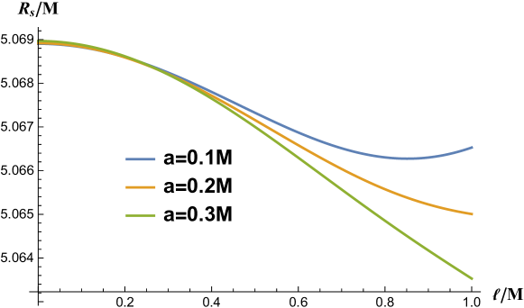
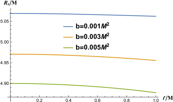
Figure 14: The left panel shows variation of $R_{s}$ with respect to $\ell$ for various values of $a$ with $b=.001M^{2}$ and $\theta=\pi/2$. The right panel shows the variation of $R_{s}$ with respect to $\ell$ for various values of $b$ with $a=0.4M$ and $\theta=\pi/2$.

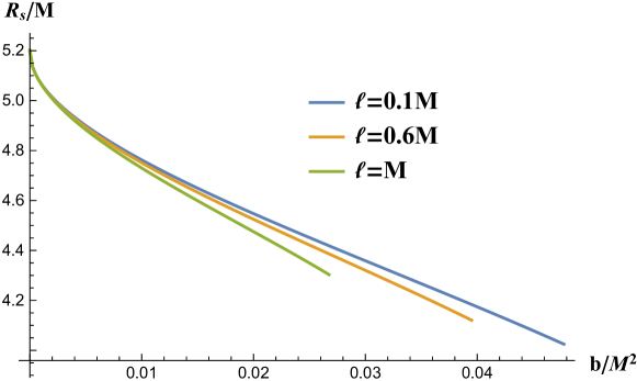
Figure 15: The left panel shows variation of $R_{s}$ with respect to $b$ for various values of $\ell$ with $a=0.1M$ and $\theta=\pi/2$.

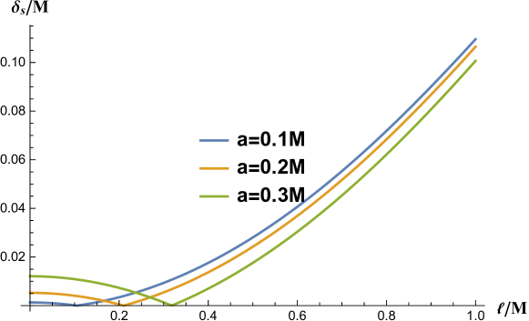
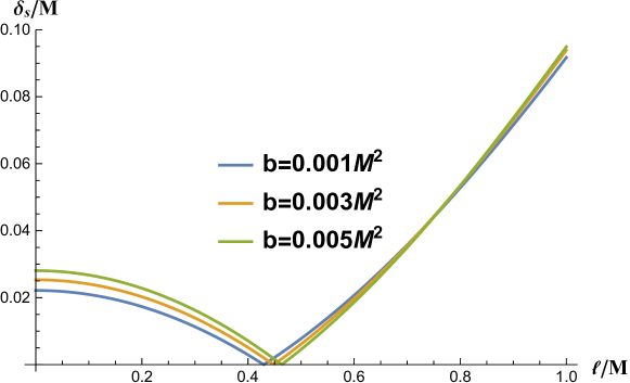
Figure 16: The left panel shows variation of $\delta_{s}$ for various values of $a$ with $b=.001M^{2}$, $\theta=\pi/2$, and the right panel shows the variation of $\delta_{s}$ for various values of $b$ with $a=0.4M$ and $\theta=\pi/2$.

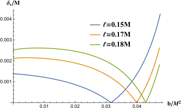
Figure 17: The left panel shows variation of $R_{s}$ for various values of $\ell$ with $a=0.1M$ and $\theta=\pi/2$.

From the above plots in Figs. (14, 15) we observe that $R_{s}$ decreases with an increase in $b$ for fixed values of $a$ and $\ell$. It is also found that $R_{s}$ decreases for an increase in the value of $a$, keeping $b$ and $\ell$ fixed or an increase in $\ell$ for fixed values of $a$ and $b$. Furthermore, it is found in Figs. (16, 17) that $\delta_{s}$ initially decreases and then increases with an increase in the value of either $\ell$ or $b$. For some specific combination of values of the parameters $a$, $b$, and $\ell$ we may get $\delta_{s}=0$. One such combination is $b=0.001$, $\ell=0.210082$, and $a=0.2M$. It signifies that for such a combination of parameters the shadow becomes a perfect circle.

VI Constraining from the observed data for $\mathrm{M}87^{*}$

In this section, an attempt is made towards constraining the parameters associated with this modified theory. We compare the geometry of the shadow obtained from the numerical computation for the Simpson-Visser black hole with the non-commutative setting with the geometry of the observed shadow for the $\mathrm{M}87^{*}$ black hole. We envisage the experimentally obtained astronomical data corresponding to deviation from circularity $\Delta\leq 0.10$ and angular diameter $\theta_{d}=42\pm 3\mu as$. The boundary of the shadow is described by the polar coordinates $(R(\phi),\phi)$ with the origin lays at the center of the shadow $(\alpha_{C},\beta_{C})$ where $\alpha_{C}=\frac{|\alpha_{max}+\alpha_{min}|}{2}$, and $\beta_{C}=0$. If a point $(\alpha,\beta)$ is considered over the boundary of the image which subtends an angle $\phi$ on the $\alpha$ axis at the geometric center ($\left(\alpha_{C},0\right)$) and the distance between the points $(\alpha,\beta)$ $\left(\alpha_{C},0\right)$ is marked by $R(\phi)$, then the average radius $R_{\text{avg}}$ of the image is given by CBK

$$R_{\text{avg}}^{2}\equiv\frac{1}{2\pi}\int_{0}^{2\pi}d\phi R^{2}(\phi),$$ (48)

where $R(\phi)\equiv\sqrt{\left(\alpha(\phi)-\alpha_{C}\right)^{2}+\beta(\phi)^{2}}$, and $\phi=tan^{-1}\frac{\beta(\phi)}{\alpha(\phi)-\alpha_{C}}$.

With this geometrical information, we have the definition of deviation from circularity $\Delta C$ TJDP :

$$\Delta C\equiv 2\sqrt{\frac{1}{2\pi}\int_{0}^{2\pi}d\phi\left(R(\phi)-R_{\text{avg }}\right)^{2}},$$ (49)

and the angular diameter of the shadow which is defined by

$$\theta_{d}=\frac{2}{d}\sqrt{\frac{A}{\pi}},$$ (50)

where $A=2\int_{r_{-}}^{r_{+}}\beta d\alpha$ is the area of the shadow. For $M87^{*}$ black hole, the distance of $M87^{*}$ from the Earth is $d=16.8Mpc$. Equations (48, 49,50 ) along with the available data for $M87^{*}$ enable us to accomplish a comparison of the theoretical predictions for modified Simpson-Visser black-hole shadows with the experimental findings provided by the EHT collaboration. In Figs. (18, 19), the deviation from circularity, $\Delta C$ is shown for the extended Simpson-Visser black holes for the two specified inclination angles $\theta=90^{o}$ and $\theta=17^{o}$ respectively.

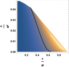
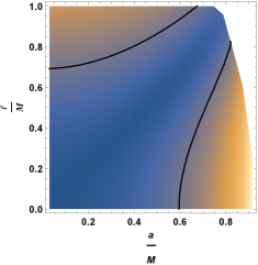
Figure 18: The left panel is for $\ell=0.1M$ and the right panel is for $b=0.001M^{2}$ where the inclination angle is $90^{o}$. The black solid lines correspond to $\Delta C=0.1$.

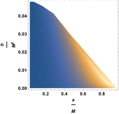
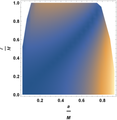
Figure 19: The left panel is for $\ell=0.1M$ and the right one is for $b=0.001M^{2}$ where the inclination angle is $17^{o}$.

In figs. (20, 21) the angular diameter $\theta_{d}$ is shown for non-commutative Simoson-Visser black holes for inclination angles $\theta=90^{o}$ and $\theta=17^{o}$ respectively.

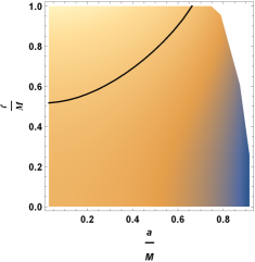
Figure 20: The left panel is for $\ell=0.1M$ and the right panel is for $b=0.001M^{2}$ where the inclination angle is $90^{o}$. The black solid lines correspond to $\theta_{d}=39\mu as$.

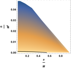
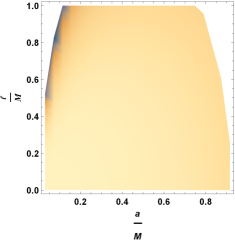
Figure 21: The left panel is for $\ell=0.1M$ and the right panel is for $b=0.001M^{2}$ where the inclination angle is $17^{o}$. The black solid lines correspond to $\theta_{d}=39\mu as$.

From Figs. (18, 19), it transpires that the constraint $\Delta C\leq 0.1$ is satisfied for finite parameter space when the inclination angle is $90^{o}$, but for $17^{o}$, the constrain is satisfied for the entire parameter space. Figs.(20, 21) reveal that for the inclination angles $\theta=90^{o}$ and $\theta=17^{o}$, the constraint $\theta_{d}=42\pm 3\mu$ is satisfied for a finite parameter space within the $1\sigma$ region. The asymmetry from the exact circular nature in the $M87^{*}$ shadow can also be determined in terms of the axial ratio $D_{X}$ which is the ratio of the major to the minor diameter of the shadow KA1 . The axial ratio $D_{X}$ is defined by BCS

$$D_{X}=\frac{\Delta Y}{\Delta X}=\frac{\beta_{t}-\beta_{b}}{\alpha_{r}-\alpha_{p}}.$$ (51)

We should have $D_{X}$ within the range $1<D_{X}\lesssim 4/3$ according to the EHT observations associated with $M87^{*}$ black hole KA1 . In fact, $D_{X}$ is defined to determine $\Delta C$ in a different manner. The measured axial ratio for $M87^{*}$ is $4:3$ which is in good agreement to $\Delta C\leq 0.1$ KA1 . In the Figs. below, axial ratio $D_{X}$ is shown for the non-commutative Simpson-Visser black hole for inclination angles $\theta=90^{o}$ and $\theta=17^{o}$ respectively.

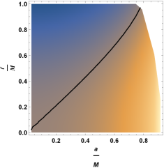
Figure 22: The left panel is for $\ell=0.1M$ and the right panel is for $b=0.001M^{2}$ where the inclination angle is $90^{o}$.

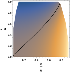
Figure 23: The left panel is for $\ell=0.1M$ and the right panel is for $b=0.001M^{2}$ where the inclination angle is $17^{o}$.

From the Figs. (22, 23), we observe that the condition $1<D_{X}\lesssim 4/3$ is satisfied for the finite parameter space of this non-commutative black hole. Thus, non-commutative Simpson-Visser black hole is remarkably consistent with EHT images of $M87^{*}$. Therefore, observational data for the $M87^{*}$ black hole shadow can not rule out the model designed for non-commutative Simpson-Visser black holes.

It would be instructive to calculate the bound of the parameter $\ell$ in a similar way we determined the bound of the Lorentz violating parameter in the paper OUR and of the non-commutative parameter $b$ in OUR1 . By modeling M$87^{*}$ black hole as Kerr black hole, the author of the paper RODRIGO obtained a lower limit of $a$ for the M$87^{*}$ black hole. Bringing this result under consideration in OUR1 we kept the interval of interest for $a$ as $[0.50M,0.99M]$, and used the experimental constraints $\Delta C\leq 0.10$ and $\theta_{d}=42\pm 3\mu as$. with these informations we observed that $b\in[0,0.000505973M^{2}]$ OUR1 . In a similar way, taking into account the bounds $a\in[0.50M,0.99M]$ and $b\in[0,0.000505973M^{2}]$ and the experimental constraints $\Delta C\leq 0.1$ and $\theta_{d}=39\pm 3\mu as$, we get a bound on the parameter $\ell$. We find that the parameter $\ell\in[0.827158M,0.85739801M]$. It is intriguing to have upper and lower bounds of $\ell$ which are found to be $0.827158M$ and $0.85739801M$ respectively. To the best of our knowledge, the bound of the parameter $\ell$ from the shadow of the astronomical black hole has not yet been reported so far.

VII Summary and Conclusion

In this paper, we have considered the black hole associated with the Simpson-Visser spacetime background augmented with the quantum correction due to the non-commutative aspect of spacetime. Although Lorentz violation is inherent in the non-commutative framework, the way this non-commutative correction is employed here the Lorentz symmetry remains undisturbed. Considering the quantum corrections gained due to the non-commutativity of spacetime, we study two important optical phenomena near this extended Simpson-Visser background: superradiant scattering and shadow cast. We begin our study with a description of the geometrical aspects regarding the horizon and ergosphere of this modified metric. We have thoroughly studied the cases when a black hole exists and when it will represent a naked singularity for this type of improved background. Graphically these are presented in Fig. (2) and we have sketched the ecospheres for different values of the parameters associated with this modified spacetime background in Fig. (3).

After giving the outline of the geometry of the modified spacetime, we move on to study the superradiance phenomena corresponding to the black hole associated with this modified spacetime metric. We observe that parameters $\ell$ and $b$ involved in the metric have a pivotal role in the superradiance scattering along with its dependence on the parameter $a$ linked with the spin of the black hole. We observe that with the increase in the value of $a$ the superradiance process intensifies. Also, the superradiance process enhances with the increase in the value of $\ell$ and the reverse is the case when the value of the parameters $a$ and $\ell$ decreases. We strikingly observe that with the increase in the value of the parameter $b$ the superradiance process gets diminished. The parameter $b$ is associated with the non-commutative aspect of spacetime and it is considered a quantum correction like the Lorentz violation parameter recently studied in OUR1 . In the non-commutative Simpson-Visser black hole, we notice the diminishing effect of quantum correction superradiance phenomena. Note that the effect of quantum correction in the superradiance associated with the violation of Lorentz symmetry that set foot in the picture through the bumblebee field was also of diminishing nature OUR1

Through numerical simulation, we develop the shadow of this modified black hole from the theoretical imputes associated with the shadow. With the apprehension that the shadow of the $M87^{*}$ is equivalent to the shadow of this quantum corrected Simpson-Visser black hole, we make an attempt to put constraint on the value of the parameter $\ell$ involved in this modified spacetime. We notice that the experimental constraint $\Delta C\leq 0.1$ is satisfied for finite parameter space when the inclination angle is $90^{o}$, but for the inclination angle $17^{o}$, the said experimental constrain is satisfied for the entire parameter space. However, the constraint $\theta_{d}=42\pm 3\mu$ is found to satisfy a finite parameter space within $1\sigma$ region for both the inclination angles $\theta=90^{o}$ and $\theta=17^{o}$. Furthermore, we observe that the measured axial ratio $4:3$ for $M87^{*}$ black hole is in good agreement with $\Delta C\leq 0.1$ for this setup.

It is intriguing if the bounds of the parameter $\ell$ can be determined from the experimental observation of astronomical black hole shadow. We have been able to estimate both the upper and lower bounds of $\ell$ from our analysis. The upper bound of $\ell$ is found to be $0.827158M$ and $0.85739801M$ is found as the lower of $\ell$. To the best of our knowledge, the estimation of the bond of the parameter $\ell$ from the astronomical findings has not yet been reported so far. In OUR1 , we gave an estimate of the lower and upper bounds of $b$. Here also, both the upper and lower bounds of $\ell$ have been possible to determine from the findings of the astronomical black hole $M87^{*}$. It would be attention-grabbing if it has been possible to estimate these bounds from the observation of $SgrA^{*}$ and to what extent it agrees with the present one.

References

- (1) Y. B. Zel’dovich Pis’ma Zh. Eksp. Teor. Fiz. 14 (1971) 270 [JETP Lett. 14, 180 (1971)].
- (2) Y. B. Zel’dovich Zh. Eksp. Teor. Fiz 62 (1972) 2076 [Sov.Phys. JETP 35, 1085 (1972)].
- (3) A. A. Starobinsky, Zh. Eksp. Teor. Fiz. 64, 48 (1973) [Sov.Phys. JETP 37, 28 ( 1973)]
- (4) A. A. Starobinsky and S. M. Churilov:Zh. Eksp. Teor. Fiz. 65, 3 (1973) [Sov. Phys. JETP 38, 1 (1973)].
- (5) W.H. Press, S.A. Teukolsky,.: Nature 238, 211-212 (1972)
- (6) S. A. Teukolsky, W. H. Press: Astrophys. J. 193 443 (1974)
- (7) R. Brito, V. Cardoso, P. Pani: Lecture Notes in Physics (2nd edition) 971 (2020)
- (8) S. Hawking, Commun.Math.Phys. 43 (1975) 199
- (9) A. Arvanitaki, S. Dimopoulos, S. Dubovsky, N. Kaloper, and J. March-Russell, Phys.Rev. D81(2010) 123530,
- (10) A. Arvanitaki, S. Dubovsky, Phys.Rev. D83 (2011) 044026,
- (11) P. Pani, V. Cardoso, L. Gualtieri, E. Berti, A. Ishibashi, Phys.Rev.Lett. 109 (2012) 131102,
- (12) R. Brito, V. Cardoso, P. Pani, Phys. Rev. D88 (2013) 023514
- (13) C. A. R. Herdeiro and E. Radu, Phys.Rev.Lett. 112 (2014) 221101,
- (14) V. Cardoso and O. J. Dias, Phys.Rev. D70 (2004) 084011,
- (15) O. J. Dias, P. Figueras, S. Minwalla, P. Mitra, R. Monteiro, et al. JHEP 1208(2012) 117
- (16) O. J. Dias, G. T. Horowitz, and J. E. Santos, JHEP 1107 (2011) 115,
- (17) M. Shibata and H. Yoshino, Phys. Rev. D81 (2010) 104035,
- (18) J. L. Synge: MNRAS 131 463 1966.
- (19) J. P. Luminet: Astronmy and Astrophysics, 75, 228 (1979).
- (20) S. Chandrasekhar, The Mathematical Theory of Black Holes, Oxford University Press, New York, (1992)
- (21) K. Hioki and K. I. Maeda: Phys. Rev. D80, 024042 (2009).
- (22) T. Johannsen, D. Psaltis: Astrophys. J. 718, 446 (2010).
- (23) K. Akiyama et al.: Astrophys. J. 875, L1 (2019).
- (24) K. Akiyama et al.: Astrophys. J. 875, L2 (2019).
- (25) K. Akiyama et al.: Astrophys. J. 875, L3 (2019).
- (26) K. Akiyama et al.: Astrophys. J. 875, L4 (2019).
- (27) K. Akiyama et al.: Astrophys. J. 875, L5 (2019).
- (28) K. Akiyama et al.: Astrophys. J. 875, L6 (2019).
- (29) H. Davoudiasl, P. B. Denton: Phys. Rev. Lett. 123, 021102 (2019)
- (30) Y. Meng, X. M. Kuang, Zi-Yu Tang: arXiv:2204.00897
- (31) M. Khodadi, G. Lambiase, D. F. Mota: JCAP 09 028 (2021)
- (32) M. Khodadi, E. N. Saridakis: Phys.Dark Univ. 32 100835 (2021)
- (33) M. Khodadi, A. Allahyari, S. Vagnozzi, David F. Mota: JCAP 2009 026 (2020)
- (34) T. Kawashima, M. Kino, K. Akiyama Astro-phys. J. 878 27 (2019)
- (35) R. J. Szabo: Phys. Rept. 378 207 (2003)
- (36) S. M. Carroll, J. A. Harvey, V. A. Kostelecky, C. D. Lane, T. Okamoto: Phys. Rev. Lett. 87, 141601 (2001)
- (37) Jian Jing, Ling-Bao Kong, Qing Wang, Shi-Hai Dong: Phys.Lett. B808 135660 (2020)
- (38) S. Bhattacharyya, S. Gangopadhyay, A. Saha: Class.Quant.Grav. 36 055006 (2019)
- (39) R. Fresneda, D.M. Gitman, A. E. Shabad: Phys.Rev. D91 085005 (2015)
- (40) C. B Luo, F. Y. Hou, Z. F Cui, X. J. Liu, H. S. Zong: Phys.Rev. D91 036009 (2015)
- (41) P. Nicolini: Int. J. Mod. Phys. A 24, 1229 (2009)
- (42) P. Aschieri, C. Blohmann, M. Dimitrijevic, F. Meyer, P. Schupp, J. Wess: Class. Quant. Grav. 22, 3511 (2005)
- (43) P. Aschieri, M. Dimitrijevic, F. Meyer, J. Wess: Class. Quant. Grav. 23, 1883 (2006)
- (44) S. Meljanac, A. Samsarov, M. Stojic, K. S. Gupta: Eur. Phys. J. C 53, 295 (2008)
- (45) E. Harikumar, T. Juric and S. Meljanac: Phys. Rev. D 86, 045002 (2012)
- (46) D. Mattingly: Living Rev. Rel. 8, 5 (2005)
- (47) A. Smailagic, E. Spallucci, J. Phys. A 36 (2003) L467
- (48) A. Smailagic, E. Spallucci, J. Phys. A 36 (2003) L517
- (49) A. Smailagic, E. Spallucci J.Phys. A37 1 (2004); Erratum-ibid. A37 7169 (2004)
- (50) P. Nicolini, A. Smailagic, E. Spallucci, Phys. Lett. B 632 547 (2006)
- (51) K. Nozari and S. H. Mehdipour: Class. Quant. Grav. 25, 175015 (2008)
- (52) W. Kim, E. J. Son, M. Yoon: JHEP 0804, 042 (2008)
- (53) K. Nozari, S. H. Mehdipour: JHEP 0903, 061 (2009)
- (54) R. Banerjee, B. R. Majhi and S. Samanta: Phys. Rev. D77, 124035 (2008)
- (55) S. H. Mehdipour: Commun. Theor. Phys. 52, 865 (2009)
- (56) S. H. Mehdipour: Phys. Rev. D 81, 124049 (2010)
- (57) Y. G. Miao, Z. Xue and S. J. Zhang: Gen. Rel. Grav. 44, 555 (2012)
- (58) K. Nozari and S. Islamzadeh: Astrophys. Space Sci. 347, 299
- (59) A. Ovgun and K. Jusufi: Eur. Phys. J. Plus 131 177 (2016)
- (60) K. S. Gupta, T. Juric, A. Samsarov: JHEP 1706, 107 (2017)
- (61) G. D. Barbosa, N. Pinto-Neto: Phys.Rev. D70 103512 (2004)
- (62) M. Marcolli E. Pierpaoli : arXiv:0908.3683
- (63) M. Marcolli, E. Pierpaoli, K. Teh: Commun. Math. Phys. 309 341 (2012)
- (64) M. Khodadi, K. Nozari, F. Hajkarim: Eur. Phys. J. C 78 716 (2018)
- (65) A. Touati, S. Zaim: arXiv:2204.01901
- (66) J. Liang and B. Liu: Eur. Phys. Lett. 100, 30001 (2012)
- (67) K. Bakke H. Belich: Eur. Phys. J. Plus 129: 147 (2014).
- (68) V. A. Kostelecky, C. D. Lane: Journal of Mathematical Physics 40, 6245 (1999).
- (69) T. J. Yoder and G. S. Adkins: Phys. Rev. D 86, 116005 (2012).
- (70) R. Lehnert: Phys. Rev. D 68, 085003 (2003).
- (71) O. G. Kharlanov, V. Ch. Zhukovsky: J. Math. Phys. 48, 092302 (2007).
- (72) V. A. Kostelecky and M. Mewes: Phys. Rev. Lett. 87, 251304 (2001).
- (73) V. A. Kostelecky and M. Mewes: Phys. Rev. D 66, 056005 (2002).
- (74) V. A. Kostelecky and M. Mewes: Phys. Rev. Lett. 97, 140401 (2006).
- (75) V. A. Kostelecky and M. Mewes: Phys. Rev. Lett. 87, 251304 (2001).
- (76) S. Carroll, G.B. Field, and R. Jackiw: Phys. Rev. D 41, 1231 (1990).
- (77) C. Adam and F. R. Klinkhamer: Nucl. Phys. B 607, 247 (2001).
- (78) W. F. Chen and G. Kunstatter: Phys. Rev. D 62, 105029 (2000).
- (79) C. D. Carone, M. Sher, M. Vanderhaeghen: Phys. Rev. D74, 077901 (2006).
- (80) F.R. Klinkhamer and M. Schreck: Nucl. Phys. B848, 90 (2011).
- (81) M. Schreck: Phys. Rev. D86, 065038 (2012).
- (82) M. A. Hohensee, R. Lehnert, D. F. Phillips, R. L. Walsworth: Phys. Rev. D80, 036010 (2009).
- (83) B. Altschul and V. A. Kostelecky: Phys. Lett. B628, 106.
- (84) R. Bluhm, N. L. Gagne, R. Potting, A. Vrublevskis: Phys. Rev. D 77, 125007 (2008).
- (85) R. Bluhm, V. Alan Kostelecky: Phys. Rev. D71, 065008 (2005).
- (86) R. V. Maluf, V. Santos, W. T. Cruz, C. A. S. Almeida: Phys. Rev. D88, 025005 (2013).
- (87) R.V. Maluf, C.A.S. Almeida, R. Casana, M.M. Ferreira, Jr.: Phys. Rev. D 90 025007 (2014)
- (88) Q. G. Bailey and V. A. Kostelecky: Phys. Rev. D74, 045001 (2006).
- (89) V. A. Kostelecky, S. Samuel: Phys. Rev. D39 683 (1989).
- (90) V. A. Kostelecky, S. Samuel: Phys. Rev. Lett. 63, 224 (1989).
- (91) V. A. Kostelecky, S. Samuel: Phys. Rev. D 40, 1886 (1989).
- (92) D. Colladay and V. A. Kostelecky: Phys. Rev. D 55, 6760 (1997)
- (93) D. Colladay, V.A. Kostelecky: Phys. Rev. D 55, 6760 (1997); Phys. Rev. D 58, 116002 (1998)
- (94) V. A. Kostelecky: Phys. Rev. D69, 105009 (2004)
- (95) D. Colladay, V.A. Kostelecky: Phys. Rev. D 55, 6760 (1997).
- (96) D. Colladay, V.A. Kostelecky: Phys. Rev. D 58, 116002 (1998)
- (97) C. Ding, C. Lui, R. Casana: A. Cavalcante: Eur. Phys. J. C80 178 2020.
- (98) R. Casana and A. Cavalcante: Phys. Rev. D 97, 104001 (2018).
- (99) S. K. Jha, A. Rahaman: Euor. Phys. J. C
- (100) J.A. Wheeler, Relativity, Groups, and Topology, edited by C. DeWitt and B. DeWitt (Gordon and Breach, New York, 1964).
- (101) A.D. Sakharov, Sov. Phys. JETP, 22, 241 (1966).
- (102) E.B. Gliner, Sov. Phys. JETP, 22, 378 (1966).
- (103) J. Bardeen, in Proceedings of GR5 (Tiflis, U.S.S.R., 1968)
- (104) A. Simpson and M. Visser, JCAP 02, 042 (2019)
- (105) A. Simpson, P. Martin-Moruno and M. Visser, Class. Quant. Grav. 36, 145007 (2019)
- (106) F. S. N. Lobo, M. E. Rodrigues, M. V. d. S. Silva, A. Simpson, M. Visser: Phys. Rev. D 103, 084052 (2021)
- (107) J. Mazza, E. Franzin and S. Liberati, JCAP 04, 082 (2021)
- (108) R. Carballo-Rubio, F. Di Filippo, S. Liberati, M. Visser, Phys. Rev. D 101 084047(2020)
- (109) P. Nicolini, Int. J. Mod. Phys. A 24 (2009) 1229
- (110) R.J. Szabo, Class. Quantum Gravity 23 (2006) R199
- (111) M. A. Anacleto, F. A. Brito, J. A. V. Campos, E. Passos: Phys. Lett. B803, 135334 (2020)
- (112) R. Penrose: Riv. Nuovo Cim. 1, 252 (1969).
- (113) D. N. Page: Phys. Rev. D13 198 (1976)
- (114) Ran Li: Phys. Lett. B714 337 (2012)
- (115) M. Khodadi: Phys.Rev. D103, 064051 (2021)
- (116) F. Atamurotov, B. Ahmedov, A. Abdujabbarov: Phys. Rev. D92, 084005 (2015).
- (117) V. Perlick, O. Y. Tsupko: Phys. Rev. D 95, 104003 (2017).
- (118) Shao-Wen Wei, Yu-Xiao Liu: JCAP 11, 063 (2013).
- (119) G. Z. Babar, A. Z. Babar, F. Atamurotov: Euro. Phys. Jour. C80, 761 (2020).
- (120) S. Dastan, R. Saffari, S. Soroushfar: arXiv:1610.09477
- (121) R. Casana, A. Cavalcante, F. P. Poulis, E. B. Santos: Phys. Rev. D 97, 104001 (2018)
- (122) A. H. Klotz, Gen. Gel. Grav. 14, 727 (1982)
- (123) S. K. Jh, H. Barman, A. Rahaman: JCAP 2104 036 (2021)
- (124) B. Mashhoon: Phys. Rev. D7, 2807 (1973)
- (125) A. Abdujabbarov, M. Amir, B. Ahmedov, S. G. Ghosh: Phys. Rev. D93, 104004 (2016)
- (126) A. Rogers: MNRAS, 451 17 2015
- (127) C. Bambi, K. Freese, S. Vagnozzi, L. Visinelli: Phys.Rev.D100 044057 (2019).
- (128) S. Kanzi, I. Sakalli: Eur. Phys. J. C 82 93 2022
- (129) S. Hod, Phys. Lett. B 708 320 (2012)
- (130) V. B. Bezerra, H. S. Vieira, A. A. Costa: Class.Quantum Grav. 31 045003 (2014)
- (131) G. V. Kraniotis: Class.Quant.Grav. 33 225011 (2016)
- (132) I. Banerjee, S. Chakraborty, S. Sengupta: Phys. Rev. D101, 041301 (2020).
- (133) S. K. Jha, S. Aziz, A. Rahaman: Eur. Phys. J. C 82 106 2022
- (134) R. Nemmen: Astrophys J. Letts L26 880 (2019)
- (135) S. K. Jha, A. Rahaman: Eur. Phys. J. C 82 728 (2022)