Analysis and Estimation of Consumer Expenditure assuming uniform prices across FSUs: A step towards cost effectiveness

Abstract

Analysis and estimation of consumer expenditure and budget shares are important for understanding quantitatively the expenditure based behaviour of the people of a country or region. The costs attached with performing consumer expenditure and budget shares survey are significant. These surveys are quite time consuming and even a slight increase in sample size could lead to a significant increase in the cost of the survey under the current structure. This high cost for the survey also reduces its flexibility. Hence it is of paramount importance to be able to provide a statistically sound and relatively cheaper facilitation method of survey to be able to understand the consumption expenditure distribution of a country or a region without much loss of inferential power. In the context of the Indian National Sample Survey, in this paper we perform analysis and estimation of consumer expenditure assuming uniform prices across First Stage Units (FSUs) of a sampling design, and check its feasibility in estimating the consumer expenditure distribution of the country. We also compare it with the existing methodology and infer that there is no significant loss of information in the estimated consumer expenditure distribution and other inferences like the Lorenz curve and the Gini Index, when uniform distribution of prices within any FSU is assumed.

Keywords: Consumer Expenditure, FSU (First Stage Unit), cost effective survey, AIDS, elasticity, Lorenz curve

1 Introduction

Analysis and estimation of consumer expenditure and budget shares are an important process which helps us understand quantitatively the expenditure based behaviour of the people of a country or region. Analysis of consumption expenditure is important for understanding short term as well as long term economic phenomena because consumption expenditure to a huge degree can demonstrate fluctuations in various important economic factors which in turn helps us perceive it as an expression of economic stability and health. Even a small decrease in consumption expenditure can damage the economy and hence it is quite important to be able to understand and precisely quantify as well as analyse the consumption expenditure distribution of a country or a region of interest. Krishnaswamy (2012) provide excellent examples of the utility of expenditure surveys. The paper comments on the various insights which can be drawn from the consumer expenditure surveys, such as the growth of GDP and other relevant economic factors.

Sen (2000), Ghosh et al. (2011) and Sen (2001) are important papers which touch upon the subjects of distribution of the consumer expenditure of the people of India. These papers emphasize the need of statistical analysis of consumer expenditure behaviour and study the various facets of the consumer expenditure distribution and their implications towards the economy and the society in general. These papers also touch upon the methodology corresponding to the collection of data through the surveys conducted by the Indian National Sample Survey Organization (NSSO) and also gives us an idea about the shortcomings and the cost of such surveys. Sen (2000) also mentions the costs attached while performing consumer expenditure and budget shares survey and its implications towards statistical reliability, because with the current setup of collecting a large amount of data from every household, achieving statistically sound survey data is often quite time consuming and an increase in sample size would lead to a huge increase in the cost of the survey under the current design. Hence it is of paramount importance to be able to provide a statistically sound and relatively cheaper method for facilitation of survey, to be able to understand the consumption expenditure distribution of a country or a region without much loss of inferential strength. Seshadri (2019) states that in 2017, the CES report was withheld citing bad data quality. The Ministry said “Concerns were also raised about the ability/sensitivity of the survey instrument to capture consumption of social services by households especially on health and education. The matter was thus referred to a committee of experts which noted the discrepancies and came out with several recommendations including a refinement in the survey methodology.” Hence the need of a robust and cheap method of survey with a sound statistical basis is vital.

Understanding and modelling of consumer expenditure as well as the corresponding budget share has been an important part of the economic literature. Many models have been proposed to analyse and understand the budget share corresponding to various commodities for a given family or households. Deaton and Muellbauer (1980) provides an excellent review of the various tools which have been used throughout the years for consumer expenditure and budget share estimation and analysis. The various models range from simple classical models such as the linear expenditure system or the Rotterdam system to more complex models such as the Almost Ideal Demand System (AIDS model). Applications of the AIDS model is quite popular for studying consumption behaviour and consumption modelling and has been widely used as in Syriopoulos and Thea Sinclair (1993), Fan et al. (1995), Yang and Koo (1994) and Ahmed and Shams (1994) which presents many interesting applications of the model and highlights many of its utilities.

We have also introduced measurement error correction in our model structure under a cross validation setup to be able to generalise our observations by incorporating errors in measurement in both the prices observed of the various items considered in the surveys and total expenditure, using tools described in Nab et al. (2021b) and Nab and Groenwold (2021). Berger et al. (2000), Klepper and Leamer (1984) and Hyslop and Imbens (2001) provide the conceptual framework and also outlines the necessity for inclusion of classical error measurement and its analysis with respect to our model and creation of the corresponding statistical framework. Griliches and Hausman (1986) also inspires a lot of the analysis performed here towards creation of a generalised model with more flexibility and interpretability.

In this paper we perform analysis and estimation of consumer expenditure assuming uniform prices across FSU’s. We can easily understand that if we assume uniform prices across FSU’s then the amount of data that would be required in the survey would be much less than in the case of every household in the FSU being asked about the prices. Hence we try to understand the statistical reliability of replacing all the individual values of prices in a given FSU by one of the prices from the set of households, considering it as a representative of the prices for the entire FSU. In this paper a modified version of the AIDS model, considering measurement errors in data collected corresponding to prices as well as consumption expenditure, has been used to understand the dissimilarities/similarities in the obtained budget shares and total expenditures in both the usual approach of complete data collection and the approach with assuming uniform prices across FSUs. A review of the relevant literature is made in the next section. The description of data, methodology and results obtained under alternative assumptions are discussed over several subsections of section 3. In particular, we analyse the robustness of our results in the presence of measurement error in a very general setting.

Apart from the budget share, two other very important metrics in the context of the CEs are measurement of inequality and demand elasticity. The Lorenz curve and the Gini Index are two most well known measures of inequality. Section 4 looks at the related issue of the estimation of the Lorenz curve and the Gini Index in the usual as well as our proposed approach. Similar analysis for demand elasticity is carried out in Section 5. Finally section 6 concludes the paper.

2 Literature Review

Consumer Expenditure models (CEMs) are widely studied due to the interpretation it provides to the household expenditure as a function of various budget shares and prices of commodities. Various economic models for consumer analysis have been proposed and implemented over the years. One of the first empirical model was the Working-Leser model. The original form of the Working-Leser model was discussed by Working (1943) and Leser (1963), with recent implementation in Karunakaran and Ahmad (1996), Brosig (2000), Chern et al. (2002) and Yeong-Sheng (2008). Intriligator et al. (1996) and Deaton and Muellbauer (1980) also discuss these functional forms as well as describe modifications and implementations on real life data. Amemiya (1985) and Maddala (1983) study the Tobit and Heckman’s two-step estimator Heckman et al. (2003), which is another important estimator which improves on the Working-Leser model structure. McDonald and Moffitt (1980) also deals with this model and improves upon the understanding of the model structure.

Deaton and Muellbauer (1980) created an efficient and flexible demand system AIDS, which stands for ’Almost Ideal Demand System’. It is not just extremely popular but also extremely versatile. The notion of a flexible demand system comes in handy when evaluating a demand system with a lot of desired characteristics. The AIDS model, as Moschini (1998) and Henningsen (2017) point out, meets the aggregation limitation, and provides facility to test and impose the homogeneity and symmetry with simple parametric requirements. Furthermore, the non-linear Engel curves of the AIDS model suggest that when income rises, the percentage of income devoted to a given commodity decreases, as does the income elasticity of that product when it is less than one. It also satisfies the axioms of choice, is an arbitrary first-order approximation to any demand system. The functional form of AIDS is still widely used in recent publications (see, e.g. Brännlund et al. (2007); Chambwera and Folmer (2007); Farrell et al. (2007); and also Ahmed and Shams (1994) among many others)

Henningsen (2017) is an important contribution towards implementation of the AIDS models as it itself states -”The aim of this paper is to describe the tools for demand analysis with the AIDS that are available in the R (R Development Core Team 2008) package micEconAids (version 0.5).” Henningsen (2017) implements both the AIDS as well as the LA-AIDS models in R while highlighting modifications. This paper uses this package extensively for its usefulness and efficient functionalities.

Measurement error was also included in this study to be able to generalise the model structure and widen the scope of the analysis. Fuller (2009) is an excellent primer in the field of error measurement analysis. Griliches and Hausman (1986) provides the R framework towards incorporating measurement errors in the consumer expenditure model structure. Nab and Groenwold (2021) is one of the most recent works in this domain. Some important works in this domain are Angrist and Keueger (1991), Aigner (1973), Card (1996), Ashenfelter and Krueger (1994) and Berger et al. (2000). Some other notable publications include on various applications of measurement error based methodolgies are Bound et al. (1994), Kane et al. (1999). Klepper and Leamer (1984) and Hyslop and Imbens (2001) are some important works in this field and provide excellent insights toward applications of measurement error analysis.

Wahba and Wendelberger (1980) provides motivation towards Variational objective analysis using splines and cross validation. Pischke, Steve (2007) is an excellent source, and provides a comprehensive primer towards understanding Measurement errors. We used the package Nab et al. (2021a) for the utilisation of various measurement error based methodologies into our model structure.

As defined by the U.S. Bureau of Labor Statistics Bureau of Labor Statistics (2018), ”A consumer expenditure survey is a specialized study in which the emphasis is on data related to family expenditures for goods and services used in day-to-day living. In addition to data on family expenditures, the Consumer Expenditure Survey (CES) collects information on the amount and sources of family income, changes in assets and liabilities, and demographic and economic characteristics of family members”. Bureau of Labor Statistics (2018) also states the importance of CES by stating ”Data also are used by economic policymakers interested in the effects of policy changes on levels of living among diverse socioeconomic groups, and econometricians find the data useful in constructing economic models.”

The utility of CEMs in understanding economic progress as well as growth quantitatively is unquestionable. Many papers, icluding recent ones, have analysed and inferred upon the state of various parameters which influence the economy, using CEMs as a primary tool in one form or the other, such as Castro et al. (2012), Sundaram-Stukel (2021), Meng et al. (2021), Dobrowolska Perry and Brown (2021), Sakai (2021), Kovács (2021), Cachola and Pacca , Dong et al. (2021) and many others.

Chandra (2021), Sen (2000), Ghosh et al. (2011), Sen (2001) highlight applications and usages of CEs in the Indian scenario, that is towards understanding the growth of the economy along with various other factors which directly affect our economy. It also shows us the changes in the economic structure across various classes of the society over a period of time, and implementations of CEMs helps us quantify the changes which occur in not just in terms of the expediture of the household, but also how the household chooses to use its income on consumption based expenditures, which in turn helps us to gain a deeper insight into the state of the Indian Economy.

3 The Demand System

3.1 Data

The data was collected from NSS (2016)-” Household Consumer Expenditure: NSS 68th Round, Schedule 1.0, July 2011 - June 2012 (type 1 ).” As NSS (2016) states-”The programme of quinquennial surveys on consumer expenditure and employment & unemployment, adopted by the National Sample Survey Organisation (NSSO) since 1972-73, provides a time series of household consumer expenditure data. Consumer expenditure surveys conducted in NSS rounds besides the ’quinquennial rounds’ - starting from the 42nd round (July 1986 - June 1987) - also provide data on the subject for the period between successive quinquennial rounds, using a much smaller sample. The sixth instance of the quinquennial series was held during the 55th round (July 1999-June 2000). The seventh was conducted in the 61st round during July 2004 - June 2005 and 66th round of NSS (2009-10) which was the eighth quinquennial survey in the series on ’household consumer expenditure’ and ’employment and unemployment’.”

The data is composed of many blocks, which include

• Block 1 : Identification of sample household.

• Block 2 : Particulars of field operations.

• Block 3 : Household characteristics.

• Block 4 : Demographic and other particulars of household members.

• Block 5.1 : Consumption of cereals, pulses, milk and milk products, sugar and salt.

• Block 5.2 : Consumption of edible oil, egg, fish and meat, vegetables, fruits, spices, beverages and processed food and pan, tobacco and intoxicants.

• Block 6 : Consumption of energy (fuel, light & household appliances).

• Block 7 : Consumption of clothing, bedding, etc.

• Block 8 : Consumption of footwear.

• Block 9 : Expenditure on education and medical (institutional) goods and services.

• Block 10 : Expenditure on miscellaneous goods and services including medical (non-institutional), rents and taxes.

• Block 11 : Expenditure for purchase and construction (including repair and maintenance) of durable goods for domestic use.

and so on. We basically focus on block 5 (5.1 & 5.2) in this study. There are 23 items that are considered in our analysis (see Table 1). There were two data components for each item, one for urban households and one for rural households. The data also consist of The household IDs (denoted by HHID), the state from which the family hails (denoted by STATE), the net quantity consumed by the household (denoted by NHQ), the net household value (denoted by NHV), the monthly per capita expenditure (denoted by MPCE), and the multiplier (denoted by MULT). We combine these data into a single data structure that contains all of the households’ ids, states, sizes, and shares of various items used by the household, as well as their prices.

item name	item number
Rice-PDS	i101
Rice-other sources	i102
Wheat/atta - other sources	i108
suji, rawa	i111
jowar, products	i115
arhar (tur)	i140
moong	i143
masur	i144
urd	i145
besan	i151
milk : liquid	i160
ghee	i164
salt	i170
sugar - other sources	i172
mustard oil	i181
refined oil [sunflower,soyabean,saffola, etc]	i184
goat meat /mutton	i192
chicken	i195
potato	i200
onion	i201
tomato	i202
banana	i220
tea : cups	i271

Table 1: Items and their corresponding identification numbers

3.2 Fitting the model

The objectives of this paper are as follows:

1. Fitting AIDS model to our data and estimating expected shares from this model.

   $$w_{il}=\alpha_{i}+\sum_{j}\gamma_{ij}*log(p_{j})+\beta_{i}*log(x_{l}/P)+\epsilon_{il}$$ (3.1)

   for the $l^{th}$ household, under the restriction $\sum_{i}\alpha_{i}=1$, $\sum_{i}\beta_{i}=0$, $\sum_{i}\gamma_{ij}=0$, $\sum_{j}\gamma_{ij}=0$ and $\gamma_{ij}=\gamma_{ji}$ for all i and j.

2. Creating an alternate data set from the original one by making the price of an item constant in each FSU and checking the distributional similarity of shares with the one estimated above.

3. Checking the same distributional similarity as explained in 2, taking into account state effects. Hence this provides a generalisation to the model setup already used for structuring the consumer expenditure data.

4. Checking the same distributional similarity as explained in 2, taking the total expenditure and prices as random effects. This provides a further improvement to our model setup, and helps us further obtain a generalised data structure.

We use R package ”micEconAids” to fit the above model. One can refer to papers such as Henningsen (2011) and Henningsen (2017) for better understanding of the package and its specifications.

3.3 Distributional similarity of shares under the assumption of equality of prices in each FSU

Households with same HHIDs except the last 2 digits falls under the same FSU. First we fit our AIDS model to the original dataset. Now micEconAids (Henningsen (2017)) package drops a row of the data matrix even if one element of it is NA. We have chosen a pool of 6 items with the least amount of NA entries in them among all the 23 items (2.4%, 5.3%, 9.7%, 9.9%, 12.8% and 14% of the entries corresponding to these items are NA respectively) using which we can estimate their shares most accurately by this package. The items turned out to be i202, i160, i108, i143, i220 and i200. We find their expected shares $(w_{i}^{1})$. Next we create a new dataset where all the item prices in each FSU is constant. We refit our model for this new dataset using only the above mentioned items and evaluate the expected shares$(w_{i}^{2})$. We check if $w_{i}^{1}$ has the same distribution as $w_{i}^{2}$.

We do a 2-sample both sided Kolmogorov-Smirnov (KS) test on the individual components of $w_{i}^{\prime}s$. There are 6 consumption items. For i160, i143 and i200 the hypothesis was accepted and in all other case it was rejected at 5 % significance level. The results obtained for the KS test are shown in table 2 (columns 3 & 4).

		w.o. state effect		with state effect
item	D	p-value	Accept/Reject	p-value	Accept/Reject
i108	0.043197	$1.099\times 10^{-7}$	Reject	0.4944	Accept
i143	0.012725	0.4628	Accept	0.3086	Accept
i160	0.012167	0.5221	Accept	0.7811	Accept
i200	0.012948	0.4405	Accept	0.4229	Accept
i202	0.028575	0.001331	Reject	0.0007453	Reject
i220	0.05101	$1.05\times 10^{-7}$	Reject	0.4821	Accept

Table 2: K-S test with and without state effect

Next we did the same hypothesis testing on the entire share vectors rather than component wise by Cramer-test for multivariate two-sample problem. It was also rejected and so we can claim that making the prices same in all the houses of the FSU do not keep the distribution of expected share the same.

3.4 Inclusion of state effects

Inclusion of the spatial properties of consumer expenditure is an important part of the process of generalising the model for households in the data set. The main reason for the inclusion of spatial properties into the model is the fact that the consumer expenditure for various items vary from one region to another owing to people from different regions having different preferences with regards to their consumption and also due to the different practices corresponding to food and other essentials in different parts of the country. To imbibe the spatial structure into the model we consider the state effects as a factor in our model which helps us to differentiate between the consumption patterns for different states. We follow the philosophy described earlier pertaining to the use of non parametric tests for the equality of the share distribution under the generalized model structure as follows

$$w_{il}=\alpha_{i}+\sum_{j}\gamma_{ij}*log(p_{j})+\beta_{i}*log(x_{l}/P)+\S_{kl}+\epsilon^{\prime}_{ikl}$$ (3.2)

where $\S_{kl}$ is the effect of the state corresponding to the k^th state, and l^th household. To find the coefficients $\S_{k}$, we partially regress the error terms $\epsilon_{ik}$ (the residuals in eq. (3.1) with an extra index for state) w.r.t. the state effects as a factor, and we substitute the coefficients obtained from the partial regression on $\epsilon_{ik}$, $\epsilon_{ikl}=\S_{kl}+\epsilon^{\prime}_{ikl}$ in eq.(3.1), to obtain the AIDS model with state effect giving us new predicted shares $w_{i}^{\prime}$. We utilise this method to assure the fact that the restrictions are upheld in the given scenario.

The results obtained for the KS test for the same setup as before, that is using items i202, i160, i108, i143, i220 and i200, are shown in table 2 (columns 5 & 6). We now obtain extremely motivating results as 5 out of 6 items are accepted as having the same budget share distribution according to the two-sided tests

It is understood that State heterogeneity contributed a lot towards the rejection of the budget share distributional equality hypothesis in the earlier analysis.

3.5 Measurement Error only in Total Expenditure:

Consumption and expenditure data is often subject to measurement error, as already discussed in section 2. To study the effect of this feature on the conclusion of our analysis, in this section we first include measurement error in the total expenditure variable only. Suppose $x_{i}^{*}$ is the original expenditure of the i-th household but the reported expenditure is $x_{i}$. In terms of a linear model we express it as

$$log(\frac{x_{i}^{*}}{P})=\theta_{0}+\theta_{1}log(\frac{x_{i}}{P})+\epsilon_{i}$$ (3.3)

where $\Theta=(\theta_{0},\theta_{1})$ and i refers to the household. We now incorporate this model in our original AIDS model and calculate the parameters for that $\Theta$ vector which has the least error.

3.5.1 Estimation of parameters

Suppose our original model is

$$y|(X,Z)=\beta_{0}+\beta_{X}X+\beta_{Z}Z+\epsilon$$ (3.4)

But we have data on responses $Y$ and error-prone predictors $\tilde{X}$ where $\tilde{X}=\theta_{0}+\theta_{1}X+U$ where $U$ is the measurement error matrix. Assume $E(U)=0$ and $Cov(U,X)=0.$ We assume non-differential covariate measurement error. The measurement error is called ‘classical’ or ‘random’ if $\theta_{0}=0$ and $\theta_{1}=1$. In this paper, we use the term random measurement error to refer to this type of measurement error. Now let

$$y|(\tilde{X},Z)=\tilde{\beta_{0}}+\tilde{\beta_{X}}\tilde{X}+\tilde{\beta_{Z}}Z+\tilde{\epsilon}$$ (3.5)

The least square estimators of (3.5), $\hat{\tilde{\beta}}=(\hat{\tilde{\beta}}_{X},\hat{\tilde{\beta}}_{0},\hat{\tilde{\beta}}_{Z})$ are biased for $\beta$ but are consistent and unbiased estimators for $\beta\Lambda$ where $\Lambda$ is the calibration model matrix (see Buonaccorsi (2010), Nab et al. (2021a)).

Nab et al. (2021a) derives the form for the calibration model matrix as below.

$$\Lambda=\begin{bmatrix}\lambda_{\tilde{X}}&\lambda_{0}&\lambda_{Z}\\ 0&\lx@intercol\hfil I\hfil\lx@intercol\end{bmatrix}$$

where $I$ is a $(k+1)*(k+1)$ identity matrix, 0 is a $(1+k)*1$ null matrix and $\lambda_{Z}$ is a $1*k$ matrix where $X$ is a k length vector and $Z$ is a $k$ length vector. It follows that $\hat{\tilde{\beta}}\Lambda^{-1}$ are consistent and unbiased estimators for $\beta.$ This understanding helps us to derive the $\Lambda$ matrix in terms of $\theta_{0}$ and $\theta_{1}$ as follows.

From (3.1) we have

$$\begin{split}E(w_{il})=\tilde{\alpha_{i}}+\sum_{j}\tilde{\gamma_{ij}}*log(p_{j})+E(\tilde{\beta_{i}}*log(\tilde{x_{l}}/P))\\ =\tilde{\alpha_{i}}+\sum_{j}\tilde{\gamma_{ij}}*log(p_{j})+\tilde{\beta_{i}}*(\theta_{0}+\theta_{1}log(\frac{x_{i}}{P}))\\ ={\alpha_{i}}+\sum_{j}\gamma_{ij}*log(p_{j})+{\beta_{i}}*log({x_{l}}/P)\end{split}$$ (3.6)

From here we can claim that $\tilde{\alpha_{i}}+\theta_{0}\tilde{\beta_{i}}=\alpha_{i},\tilde{\gamma_{ij}}=\gamma_{ij}$ and $\tilde{\beta_{i}}\theta_{1}=\beta_{1}$
Accordingly the calibration model matrix becomes $\Lambda=\begin{bmatrix}\frac{1}{\theta_{1}}&-\frac{\theta_{0}}{\theta_{1}}&0\\ 0&\lx@intercol\hfil I\hfil\lx@intercol\end{bmatrix}$

An important special case of the calibration model matrix is where we have only one response and one error prone predictor. In those situations we have $\tilde{\beta_{X}}=\lambda_{\tilde{X}}\beta_{X}$. Then $\lambda_{\tilde{X}}$ is called the attenuation factor or regression dilution factor. To be able to expand this idea and for deriving the optimal values for $\theta_{0}$ as well as $\theta_{1}$, we apply a cross-validation based approach. Cross-validation is one of the most widely used data resampling methods to estimate the true prediction error of models and to tune model parameters. Stone (1978) and Refaeilzadeh et al. (2009) are some excellent reviews of various cross-validation techniques and approaches.

We utilise 10 fold cross-validation for deriving the optimum values for $\theta_{0}$ and $\theta_{1}$. We divide the data into 10 equal parts. From $\frac{9}{10}$th of the data we estimate the values of parameters $(\beta_{0},\beta_{X},\beta_{Z})$ and then on the remaining $\frac{1}{10}$th of data we apply the trained model, obtain the estimated shares in each household and then we compute the Cross validation (CV) error as a measure of error or divergence between the estimated and the true shares. This Cross validation (CV) error is very useful for deriving or quantifying a loss function which will help us derive the values for $\theta_{0}$ as well as $\theta_{1}$ which provide us the best model parameters. The loss functions that we will be using in this context are $L_{1}$ and $L_{2}$, to implement alternative sensitivity to outliers.

3.5.2 Results

Interestingly, we find that the value of $\theta_{0}$ didn’t affect the CV error much so only the change of CV error w.r.t. the value of $\theta_{1}$ is reported here while keeping $\theta_{0}$ at 0. The set of items with minimum number of NA entries among them are i170, i200, i201 and i271. Results were obtained for these items, as shown in table 3. Best results were obtained for $\theta_{1}=1.02$ which is quite close to $1$ and since $\theta_{0}=0,$ so we can conclude that the measurement error in total expenditure is quite close to the scenario of ”classical measurement error”(3.5.1) i.e., measurement error only arises from random noise and not from any biased nature in observed total expenditures. So, the inclusion of measurement error for correcting the bias in the reported total expenditure hardly shows any improvement in the analysis.

$\theta_{1}$	CV error (L1)	CV error (L2)
0.5	873.8071	587.8226
0.6	765.0441	490.4459
0.7	582.5900	354.2595
0.8	507.0505	305.7418
0.9	4 25.4642	249.4999
0.92	396.9889	222.655
0.94	388.7303	211.9089
0.96	390.3062	207.9725
0.98	385.0477	202.5024
1	382.3179	180.2719
1.02	381.3437	178.9530
1.04	382.5989	181.904
1.06	383.2434	186.2684
1.08	383.8451	186.6432
1.1	386.8990	196.8482
1.2	389.7244	198.0584
1.3	425.8812	227.3775
1.4	460.3024	265.6682
1.5	574.4676	352.5212

Table 3: CV for measurement error analysed only for total expenditure

3.6 Measurement Error in both Prices and Expenditure:

In this section, we include measurement error in total expenditure as well as prices. In terms of a linear model we express it as

$$\begin{split}log(\frac{x_{i}^{*}}{P})=\theta_{0}+\theta_{1}log(\frac{x_{i}}{P})+\epsilon_{i}\\ log(p_{ik}^{*})=\theta_{2}+\theta_{3}log(p_{ik})+\eta_{ik}\end{split}$$ (3.7)

where $\Theta=(\theta_{0},\theta_{1},\theta_{2},\theta_{3})$, i and k refers to the household and item respectively. We next incorporate this model in our original AIDS model and obtain the parameters for that $\Theta$ vector which has the least error.

3.6.1 Estimation of parameters:

Similar to the previous section, From (3.1) we have

$$\begin{split}E(w_{il})=\tilde{\alpha_{i}}+\sum_{j}E(\tilde{\gamma_{ij}}*log(\tilde{p_{j}}))+E(\tilde{\beta_{i}}*log(\tilde{x_{l}}/P))\\ =\tilde{\alpha_{i}}+\sum_{j}\tilde{\gamma_{ij}}*(\theta_{2}+\theta_{3}log(p_{ik}))+\tilde{\beta_{i}}*(\theta_{0}+\theta_{1}log(\frac{x_{i}}{P}))\\ ={\alpha_{i}}+\sum_{j}\gamma_{ij}*log(p_{j})+{\beta_{i}}*log({x_{l}}/P)\end{split}$$ (3.8)

Hence we claim that $\tilde{\alpha_{i}}=\alpha_{i}-\frac{\theta_{0}}{\theta_{1}}\beta_{i}-\frac{\theta_{2}}{\theta_{3}}\sum_{j}\gamma_{ij},\tilde{\gamma_{ij}}=\frac{\gamma_{ij}}{\theta_{3}}$ and $\tilde{\beta_{i}}\theta_{1}=\beta_{1}.$
Accordingly the calibration model matrix becomes

$$\Lambda=\begin{bmatrix}1&0&0\\ -\frac{\theta_{0}}{\theta_{1}}&\frac{1}{\theta_{1}}&0\\ -\frac{\theta_{2}}{\theta_{3}}1&0&\frac{1}{\theta_{3}}I_{k}\end{bmatrix}$$

Now again following the Cross-Validation technique as explained before, we calculate the CV error as shown in tables 4A, 4B, 5A and 5B. Since in previous section we had obtained the result that effect of measurement error on total expenditure is negligible, we fixed $\theta_{1}=1$.

$\theta_{1}$	$\theta_{2}$	$\theta_{3}$	CV Error
1	0.045	0.975	390.7835
1	0.03	0.975	388.8978
1	0.015	0.975	386.4447
1	0	0.975	387.6745
1	-0.015	0.975	387.7026
1	-0.03	0.975	387.9214
1	-0.045	0.975	388.3474
1	0.045	0.9825	384.017
1	0.03	0.9825	383.0928
1	0.015	0.9825	385.5355
1	0	0.9825	392.1737
1	-0.015	0.9825	385.2428
1	-0.03	0.9825	386.7386
1	-0.045	0.9825	384.7865
1	0.045	1	382.3325
1	0.03	1	383.0103
1	0.015	1	383.008
1	0	1	384.6481

$\theta_{1}$	$\theta_{2}$	$\theta_{3}$	CV Error
1	-0.015	1	386.7948
1	-0.03	1	385.7552
1	-0.045	1	385.1635
1	0.045	1.0125	385.2014
1	0.03	1.0125	382.8658
1	0.015	1.0125	383.7602
1	0	1.0125	383.4262
1	-0.015	1.0125	383.9514
1	-0.03	1.0125	391.0214
1	-0.045	1.0125	382.3354
1	0.045	1.025	383.0567
1	0.03	1.025	383.3367
1	0.015	1.025	389.2024
1	0	1.025	383.2446
1	-0.015	1.025	384.9549
1	-0.03	1.025	382.2439
1	-0.045	1.025	386.6325

Table 4A: CV L1 error (item set: i170, i200, i201, i271)

$\theta_{1}$	$\theta_{2}$	$\theta_{3}$	CV Error
1	0.045	0.975	208.0036
1	0.03	0.975	205.6403
1	0.015	0.975	197.3612
1	0	0.975	202.2346
1	-0.015	0.975	200.6905
1	-0.03	0.975	197.7356
1	-0.045	0.975	197.1083
1	0.045	0.9825	196.8689
1	0.03	0.9825	193.3416
1	0.015	0.9825	196.6589
1	0	0.9825	210.8979
1	-0.015	0.9825	197.0869
1	-0.03	0.9825	195.9922
1	-0.045	0.9825	191.1388
1	0.045	1	191.6064
1	0.03	1	198.1114
1	0.015	1	195.4679
1	0	1	195.9239

$\theta_{1}$	$\theta_{2}$	$\theta_{3}$	CV Error
1	-0.015	1	201.5761
1	-0.03	1	193.2997
1	-0.045	1	196.1762
1	0.045	1.0125	194.0597
1	0.03	1.0125	196.2375
1	0.015	1.0125	197.0733
1	0	1.0125	195.814
1	-0.015	1.0125	200.0738
1	-0.03	1.0125	206.5555
1	-0.045	1.0125	195.1094
1	0.045	1.025	202.3582
1	0.03	1.025	191.3562
1	0.015	1.025	204.5542
1	0	1.025	189.7399
1	-0.015	1.025	203.9044
1	-0.03	1.025	191.532
1	-0.045	1.025	192.4589

Table 4B: CV L2 error (item set: i170, i200, i201, i271)

$\theta_{1}$	$\theta_{2}$	$\theta_{3}$	CV Error
1	0.045	0.975	447.7423
1	0.03	0.975	447.2207
1	0.015	0.975	448.0865
1	0	0.975	448.9228
1	-0.015	0.975	448.5695
1	-0.03	0.975	448.2828
1	-0.045	0.975	450.6857
1	0.045	0.9825	448.4203
1	0.03	0.9825	448.0289
1	0.015	0.9825	449.3513
1	0	0.9825	451.4599
1	-0.015	0.9825	445.6711
1	-0.03	0.9825	447.1259
1	-0.045	0.9825	447.2945
1	0.045	1	449.3804
1	0.03	1	446.9709
1	0.015	1	449.6299
1	0	1	451.5521

$\theta_{1}$	$\theta_{2}$	$\theta_{3}$	CV Error
1	-0.015	1	453.9945
1	-0.03	1	449.6805
1	-0.045	1	449.9743
1	0.045	1.0125	448.3564
1	0.03	1.0125	451.621
1	0.015	1.0125	448.5162
1	0	1.0125	446.6302
1	-0.015	1.0125	448.9254
1	-0.03	1.0125	447.3122
1	-0.045	1.0125	448.591
1	0.045	1.025	450.3971
1	0.03	1.025	448.0999
1	0.015	1.025	449.292
1	0	1.025	447.8478
1	-0.015	1.025	449.8871
1	-0.03	1.025	454.3573
1	-0.045	1.025	449.0327
1	0.45	0.9	448.2508

Table 5A: CV L1 error (item set: i102, i160, i172, i202)

$\theta_{1}$	$\theta_{2}$	$\theta_{3}$	CV Error
1	0.045	0.975	217.7359
1	0.03	0.975	217.7724
1	0.015	0.975	217.9794
1	0	0.975	219.3387
1	-0.015	0.975	218.8253
1	-0.03	0.975	218.4537
1	-0.045	0.975	220.2183
1	0.045	0.9825	218.5969
1	0.03	0.9825	219.3161
1	0.015	0.9825	219.0224
1	0	0.9825	221.2403
1	-0.015	0.9825	216.2027
1	-0.03	0.9825	218.1926
1	-0.045	0.9825	218.7398
1	0.045	1	218.9043
1	0.03	1	217.226
1	0.015	1	220.9737
1	0	1	220.3873

$\theta_{1}$	$\theta_{2}$	$\theta_{3}$	CV Error
1	-0.015	1	223.7322
1	-0.03	1	220.5439
1	-0.045	1	220.3708
1	0.045	1.0125	218.5088
1	0.03	1.0125	221.2157
1	0.015	1.0125	218.746
1	0	1.0125	217.2536
1	-0.015	1.0125	218.6351
1	-0.03	1.0125	216.8291
1	-0.045	1.0125	217.5458
1	0.045	1.025	219.5415
1	0.03	1.025	218.1658
1	0.015	1.025	218.3068
1	0	1.025	218.306
1	-0.015	1.025	220.0956
1	-0.03	1.025	223.4123
1	-0.045	1.025	218.7576
1	0.45	0.9	218.8855

Table 5B: CV L2 error (item set: i102, i160, i172, i202)

For the first set of items (which had the least number of NAs among them) (i170, i200, i201, i271) the CV L1 error and CV L2 error is minimized at $\theta=(\theta_{1},\theta_{2},\theta_{3})=(1,-0.03,1.025)$ & $(1,-0.045,0.9825)$ respectively but these points are quite close to $\theta=(1,0,1)$. We conclude from here that if we take ideal case scenario, i.e., $\theta=(1,0,1)$, it works quite well and hence there is not much significant improvement in the model considering measurement error.

Similarly, for the second set of items (i102, i160, i172, i202) (having second least number of NAs among them) both the CV L1 error and CV L2 error are minimized at $\theta=(\theta_{1},\theta_{2},\theta_{3})=(1,-0.015,0.9825)$ which is again quite close to $\theta=(1,0,1)$. Again for this set, ignoring the measurement error won’t have any significant effect on the conclusions.

Thus, overall, measurement error does not play any significant role in distorting the conclusions of our model and methodology.

4 Analysis of Inequality: Lorenz Curve and Gini Index

In the analysis above, we studied whether the alternate dataset, as explained in section 3.2, is similar to the original dataset in terms of budget share distribution. In this section we take the analysis one step further to check whether CE inequality metrics are influenced by our alternative methodology or not. We will examine this using the Lorenz Curve and the Gini Index.

We first fix an item $i.$ Corresponding to item $i$ we have information about it’s price $p_{i_{j}}$ in the $j^{th}$ household. We also know exact value of amount of the item $i$ bought in the $j^{th}$ household, $q_{i_{j}}=\frac{w_{i_{j}}Q_{j}}{p_{i_{j}}}$ where $w_{i_{j}}$ and $Q_{j}$ are respectively the share of item $i$ and total expenditure in the $j^{th}$ household. Now we draw the Lorenz curve for expenditure for item i using this original dataset.
Next we do the same but for $\tilde{p_{i_{j}}}$, the constant price for $j^{th}$ household corresponding to the FSU it belongs to. $q_{i_{j}}$ remains same here as well. We draw the Lorenz curve for the expenditure using the alternate dataset and then we compare it with previous curve. This is done for all the items that we had worked with (items $170,200,201,271,102,160,172,202$). We also compute the Gini index for these two alternatives for comparison.

The Lorenz curves for item no. 102, 170, 172, 200 are in figures 1 - 8. The right panel is for the original dataset and the left ones for alternate. As we can see, the Lorenz curves for the alternate and the original data are very close to each other, implying that our simplification do not result in any distortion.

Figure 1: i102 alternate data

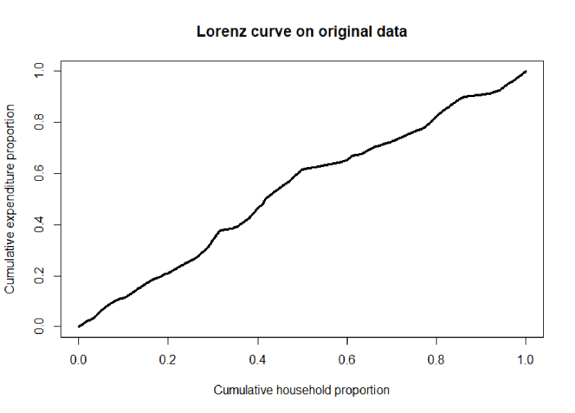
Figure 2: i102 original data

Figure 3: i170 alternate data

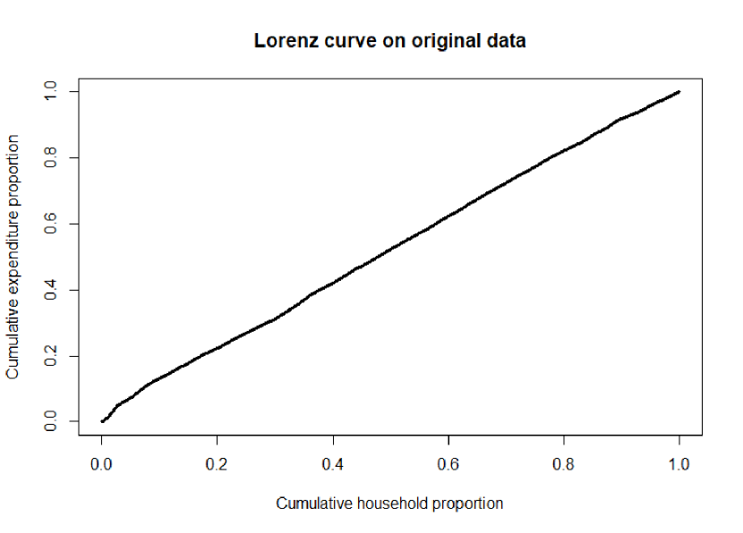
Figure 4: i170 original data

Figure 5: i172 alternate data

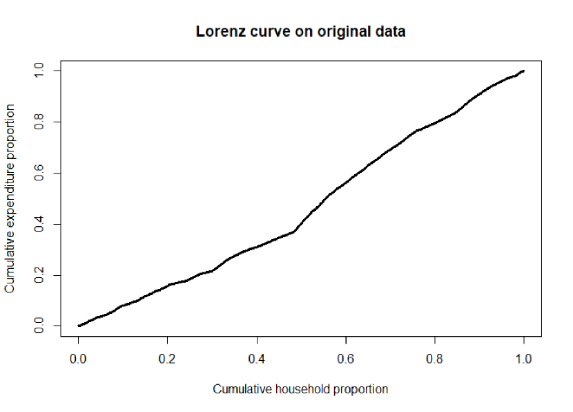
Figure 6: i172 original data

Figure 7: i200 alternate data

Figure 8: i200 original data

The Gini index for the 2 datasets is as follows (Data 1 is original, Data 2 is alternate):

item no.	Data 1	Data 2	$|\Phi(T_{1})-\Phi(T_{2})|$
102	0.447	0.452	0.05
170	0.290	0.298	0
172	0.370	0.370	0.001
200	0.407	0.418	0
201	0.358	0.366	0
202	0.383	0.394	0
271	0.390	0.408	0
160	0.411	0.409	0.003

Table 6: Gini index comparison

We make a comparison about the $significance$ of gini index difference among the 8 items. As discussed in Martínez-Camblor and Corral (2009), if $U=\{u_{1},u_{2},...,u_{n}\}$ is a random sample from a $U(0,1)$ distribution, then

$$\sqrt{n}\frac{\hat{G_{n}}-1/3}{\sqrt{8/135}}\xrightarrow[]{d}N(0,1)$$

where $\hat{G_{n}}$ is sample Gini index.
Since the data of expenditure for a item in a particular household does not necessarily follow uniform distribution, we can not apply the above result directly. We rather calculate the empirical distribution $\hat{F_{k}}$ of the expenditure of each household for item $i$ ($k$ stands for the data used). Next we define $u_{j}=\hat{F_{k}}(x_{j})$ where $x_{j}$ is the expenditure of $j^{th}$ household on item $i$ ($u_{j}\sim U(0,1)$). Now we calculate the test statistic $T_{k}=\sqrt{n}\frac{\hat{G}_{nk}-1/3}{\sqrt{8/135}}$ for both the data sets and check the value of $|\Phi(T_{1})-\Phi(T_{2})|$, where $\Phi$ is the CDF of the standard Normal distribution. If this difference is more that $0.05$, we conclude that the Gini index due to item $i$ are not statistically same for both the datas. For all our items the difference turns out to be insignificant, again proving that Data 1 and Data 2 are statistically similar to each other w.r.t. inequality in the expenditure distribution.

5 Effect on Demand Elasticity

We conclude our analysis with a comparison of demand and price elasticities (both Marshallian and Hicksian) under the AIDS model between the original and the alternate dataset.

Item number	modified dataset	original dataset	absolute difference ($10^{-3}$)
i102	1.3095478	1.3036325	5.9153
i170	0.441356	0.4351241	6.2319
i172	0.3912798	0.4053625	14.0827
i200	0.3165078	0.3040078	12.5
i202	0.2207938	0.2085229	12.2709
i271	0.2225349	0.2231390	0.6041
i160	0.3229050	0.3173401	5.5649
i220	1.0817749	1.0806154	1.1595

Table 7: Demand elasticities of 8 Items

Marshallian p_102 p_170 p_172 p_200 q_i102 -1.761 0.013 0.391 0.054 q_i170 0.898 -0.553 -0.657 -0.117 q_i172 1.593 -0.070 -1.825 -0.103 q_i200 1.481 -0.071 -0.585 -1.129 p_202 p_271 p_160 p_220 q_i202 -0.523 -0.141 -0.168 0.629 q_i271 -0.132 -0.581 -0.098 0.588 q_i160 -0.106 -0.067 -0.744 0.600 q_i220 -0.004 -0.006 -0.004 -1.066

Hicksian p_102 p_170 p_172 p_200 q_i102 -0.893 0.050 0.732 0.112 q_i170 1.182 -0.541 -0.543 -0.100 q_i172 1.863 -0.058 -1.720 -0.085 q_i200 1.683 -0.062 -0.506 -1.115 p_202 p_271 p_160 p_220 q_i202 -0.522 -0.135 -0.159 0.817 q_i271 -0.126 -0.575 -0.089 0.790 q_i160 -0.010 -0.058 -0.730 0.886 q_i220 0.024 0.025 -0.043 -0.095

Table 8A: Original Dataset

Marshallian p_102 p_170 p_172 p_200 q_i102 -1.758 0.014 0.382 0.052 q_i170 0.906 -0.467 -0.749 -0.132 q_i172 1.580 -0.079 -1.777 -0.115 q_i200 1.435 -0.079 -0.654 -1.018 p_202 p_271 p_160 p_220 q_i202 -0.395 -0.180 -0.209 0.563 q_i271 -0.165 -0.460 -0.129 0.531 q_i160 -0.129 -0.088 -0.522 0.416 q_i220 -0.006 -0.007 -0.013 -1.054

Hicksian p_102 p_170 p_172 p_200 q_i102 -0.887 0.051 0.725 0.111 q_i170 1.200 -0.455 -0.633 -0.111 q_i172 1.840 -0.068 -1.674 -0.098 q_i200 1.646 -0.070 -0.571 -1.003 p_202 p_271 p_160 p_220 q_i202 -0.389 -0.173 -0.200 0.761 q_i271 -0.159 -0.454 -0.119 0.731 q_i160 -0.120 -0.079 -0.508 0.710 q_i220 0.023 0.024 -0.035 -0.081

Table 8B: Modified dataset

As we can clearly see, the expenditure elasticities are very similar for both the data sets ($0.014$ being the maximum difference). Most of the price elasticities are also close to each other and all are of the same sign. Blue marked ones are the Marshallian price elasticities which have an absolute difference larger than $0.1$ between the two datasets and Red marked ones are the Hicksian price elasticities which have an absolute difference larger than $0.1$ between the two datasets with the maximum being 0.222. But the average difference is of a much lower order (around $0.04$). So we can conclude that our modified alternate dataset is a reasonable simplification, without any significant loss of information, of the original dataset.

6 Conclusion

Consumer Expenditure surveys are of paramount importance for macro planning for a country. Huge amount of money is spent on this every year. It would be an important contribution if a modification to existing sampling design leads to a reduction in cost with no appreciable loss of precision. This paper showed that utilising the model structure corresponding to uniform prices within FSUs does not lead to a significant loss in information for quantifying the consumer expenditure distribution as well as the associated shares as compared to the previous methodology of complete information, which in turn motivates us towards using the uniform prices setup during surveys to help in cost reduction and optimisation. We used a modified version of the AIDS (Almost Ideal Demand System) structure for quantifying the relationships between quantities of goods, total expenditure and prices under the influence of state effects and measurement errors. We have employed a Cross-Validation based technique to incorporate the optimum measurement error model for prices and total expenditure during the survey, and thus provide a generalised model structure. Due to data issues we have only been able to do the analysis for a few items. But the results were uniformly encouraging, showing no loss of information - except for one item - and no significant measurement error issues. Thus, this work paves a way towards introducing a robust and cost efficient survey methodology for Consumer Expenditure.

Our work may be extended in several directions in future. Using other general demand systems may indicate robustness of results w.r.t. model specification. Applications in the direction of measuring Poverty or Human Development may also be important in terms of policy implications. We hope that such generalisations and applications will enrich our knowledge further in this direction in the near future.

Funding source: This research did not receive any specific grant from funding agencies in the public, commercial, or not-for-profit sectors.

Declarations of interest: The authors declare no conflict of interest.

References

- NSS (2016) (2016, Sep). India - household consumer expenditure: Nss 68th round, schedule 1.0, july 2011 - june 2012 (type 1).
- Ahmed and Shams (1994) Ahmed, A. U. and Y. Shams (1994). Demand elasticities in rural bangladesh: an application of the aids model. The Bangladesh Development Studies, 1–25.
- Aigner (1973) Aigner, D. J. (1973). Regression with a binary independent variable subject to errors of observation. Journal of Econometrics 1(1), 49–59.
- Amemiya (1985) Amemiya, Y. (1985). Instrumental variable estimator for the nonlinear errors-in-variables model. Journal of Econometrics 28(3), 273–289.
- Angrist and Keueger (1991) Angrist, J. D. and A. B. Keueger (1991). Does compulsory school attendance affect schooling and earnings? The Quarterly Journal of Economics 106(4), 979–1014.
- Ashenfelter and Krueger (1994) Ashenfelter, O. and A. Krueger (1994). Estimates of the economic return to schooling from a new sample of twins. The American economic review, 1157–1173.
- Berger et al. (2000) Berger, M., D. Black, and F. Scott (2000). Bounding parameter estimates with non-classical measurement error. Journal of the American Statistical Association 95(451), 739–48.
- Bound et al. (1994) Bound, J., C. Brown, G. J. Duncan, and W. L. Rodgers (1994). Evidence on the validity of cross-sectional and longitudinal labor market data. Journal of Labor Economics 12(3), 345–368.
- Brännlund et al. (2007) Brännlund, R., T. Ghalwash, and J. Nordström (2007). Increased energy efficiency and the rebound effect: effects on consumption and emissions. Energy economics 29(1), 1–17.
- Brosig (2000) Brosig, S. (2000). A model of household type specific food demand behaviour in hungary. Technical report, Discussion paper.
- Buonaccorsi (2010) Buonaccorsi, J. P. (2010). Measurement error: Models, methods, and applications. CRC Press.
- Bureau of Labor Statistics (2018) Bureau of Labor Statistics (2018). consumer expenditures and income - bureau of labor. https://www.bls.gov/opub/hom/cex/pdf/cex.pdf.
- (13) Cachola, C. d. S. and S. A. Pacca. The carbon footprint of brazilian households through the consumer expenditure survey (pof).
- Card (1996) Card, D. (1996). The effect of unions on the structure of wages: A longitudinal analysis. Econometrica: Journal of the Econometric Society, 957–979.
- Castro et al. (2012) Castro, M., C. R. Bhat, R. M. Pendyala, and S. R. Jara-Díaz (2012). Accommodating multiple constraints in the multiple discrete–continuous extreme value (mdcev) choice model. Transportation Research Part B: Methodological 46(6), 729–743.
- Chambwera and Folmer (2007) Chambwera, M. and H. Folmer (2007). Fuel switching in harare: An almost ideal demand system approach. Energy policy 35(4), 2538–2548.
- Chandra (2021) Chandra, H. (2021). District-level estimates of poverty incidence for the state of west bengal in india: application of small area estimation technique combining nsso survey and census data. Journal of Quantitative Economics 19(2), 375–391.
- Chern et al. (2002) Chern, W. S., K. Ishibashi, K. Taniguchi, and Y. Tokoyama (2002). Analysis of food consumption behavior by japanese households.