Pressure-robust enriched Galerkin methods for the Stokes equations

Abstract

In this paper, we present a pressure-robust enriched Galerkin (EG) scheme for solving the Stokes equations, which is an enhanced version of the EG scheme for the Stokes problem proposed in [S.-Y. Yi, X. Hu, S. Lee, J. H. Adler, An enriched Galerkin method for the Stokes equations, Computers and Mathematics with Applications 120 (2022) 115–131]. The pressure-robustness is achieved by employing a velocity reconstruction operator on the load vector on the right-hand side of the discrete system. An a priori error analysis proves that the velocity error is independent of the pressure and viscosity. We also propose and analyze a perturbed version of our pressure-robust EG method that allows for the elimination of the degrees of freedom corresponding to the discontinuous component of the velocity vector via static condensation. The resulting method can be viewed as a stabilized $H^{1}$-conforming $\mathbb{P}_{1}$-$\mathbb{P}_{0}$ method. Further, we consider efficient block preconditioners whose performances are independent of the viscosity. The theoretical results are confirmed through various numerical experiments in two and three dimensions. Keywords: enriched Galerkin; finite element methods; Stokes equations; pressure-robust; static condensation; stabilization.

1 Introduction

We consider the Stokes equations for modeling incompressible viscous flow in an open and bounded domain $\Omega\subset\mathbb{R}^{d}$, $d=2,3$, with simply connected Lipschitz boundary $\partial\Omega$: Find the fluid velocity ${\bf u}:\Omega\rightarrow\mathbb{R}^{d}$ and the pressure $p:\Omega\rightarrow\mathbb{R}$ such that

$$-\nu\Delta{\bf u}+\nabla p ={\bf f} \quad\text{in }\Omega,$$ (1.1a)

$$\nabla\cdot{\bf u} =0 \quad\text{in }\Omega,$$ (1.1b)

$${\bf u} =0 \quad\text{on }\partial\Omega,$$ (1.1c)

where $\nu>0$ is the fluid viscosity, and ${\bf f}$ is a given body force.

Various finite element methods (FEMs) have been applied to solve the Stokes problem based on the velocity-pressure formulation (1.1), including conforming and non-conforming mixed FEMs [39, 5, 13, 38], discontinuous Galerkin (DG) methods [20, 17], weak Galerkin methods [30, 29], and enriched Galerkin methods [8, 42]. It is well-known that the finite-dimensional solution spaces must satisfy the inf-sup stability condition [22, 4, 6] for the well-posedness of the discrete problem regardless of what numerical method is used. Therefore, there has been extensive research to construct inf-sup stable pairs for the Stokes equations in the last several decades. Some classical $H^{1}$-conforming stable pairs include Taylor-Hood, Bernardi-Raugel, and MINI elements [16].

Though the inf-sup condition is crucial for the well-posedness of the discrete problem, it does not always guarantee an accurate solution. Indeed, many inf-sup stable pairs are unable to produce an accurate velocity solution when the viscosity is very small. More precisely, such pairs produce the velocity solution whose error bound depends on the pressure error and is inversely proportional to the viscosity, $\nu$. Hence, it is important to develop numerical schemes whose velocity error bounds are independent of pressure and viscosity, which we call pressure-robust schemes.

There have been three major directions to develop pressure-robust schemes. The first direction is based on employing a divergence-free velocity space since, then, one can separate the velocity error from the pressure error. Recall, however, that the velocity space of classical low-order inf-sup stable elements do not satisfy the divergence-free (incompressibility) condition strongly. One way to develop a divergence-free velocity space is to take the curl of an $H^{2}$-conforming finite element space [3, 14, 18], from which the pressure space is constructed by taking the divergence operator. Though this approach provides the desired pressure-robustness, it requires many degrees of freedom (DoFs). Another way, which has received much attention lately, is to employ an $H(\text{div})$-conforming velocity space [12, 41, 11, 18, 19, 10]. However, to take account of lack of regularity, the tangential continuity of the velocity vector across the inter-elements has to be imposed either strongly [18, 19] or weakly [12, 41, 11, 10]. The second direction is based on the grad-div stabilization [33, 21], which is derived by adding a modified incompressibility condition to the continuous momentum equation. This stabilization technique reduces the pressure effect in the velocity error estimate but not completely eliminates it. The third direction, which we consider in the present work, is based on employing a velocity reconstruction operator [24]. In this approach, one reconstructs ($H(\text{div})$-nonconforming) discrete velocity test functions by mapping them into an $H(\text{div})$-conforming space. These reconstructed velocity test functions are used in the load vector (corresponding to the body force ${\bf f}$) on the right-hand side of the discrete system while the original test functions are used in the stiffness matrix. This idea has been successfully explored in various numerical methods [25, 26, 15, 29, 31, 32, 40, 23].

Our main goal is to develop and analyze a pressure-robust finite element method requiring minimal number of degrees of freedom. To achieve this goal, we consider as the base method the enriched Galerkin (EG) method proposed for the Stokes equations with mixed boundary conditions [42]. This EG method employs the piecewise constant space for the pressure. As for the velocity space, it employs the linear Lagrange space, enriched by some discontinuous, piecewise linear, and mean-zero vector functions. This enrichment space requires only one DoF per element. Indeed, any function ${\bf v}$ in the velocity space has a unique decomposition of the form ${\bf v}={\bf v}^{C}+{\bf v}^{D}$, where ${\bf v}^{C}$ belongs to the linear Lagrange space and ${\bf v}^{D}$ belongs to the discontinuous linear enrichment space. To take account of the non-conformity of the velocity space, an interior penalty discontinuous Galerkin (IPDG) bilinear form is adopted. This method is one of the cheapest inf-sup stable methods with optimal convergence rates for the Stokes problem. However, like many other inf-sup stable methods, this EG method produces pressure- and viscosity-dependent velocity error. In order to derive a pressure-robust EG method, we propose to take the velocity reconstruction approach mentioned above. Specifically, the velocity test functions are mapped to the first-order Brezzi-Douglas-Marini space, whose resulting action is equivalent to preserving the continuous component ${\bf v}^{C}$ and mapping only the discontinuous component ${\bf v}^{D}$ to the lowest-order Raviart-Thomas space. This operator is applied to the velocity test functions on the right-hand side of the momentum equation, therefore the resulting stiffness matrix is the same as the one generated by the original EG method in [42]. By this simple modification in the method, we can achieve pressure-robustness without compromising the optimal convergence rates, which has been proved mathematically and demonstrated numerically.

Though the proposed pressure-robust EG method is already a very cheap and efficient method, we seek to reduce the computational costs even more by exploring a couple of strategies. First, we developed a perturbed pressure-robust EG method, where a sub-block in the stiffness matrix corresponding to the discontinuous component, ${\bf u}_{h}^{D}$, of the velocity solution ${\bf u}_{h}={\bf u}_{h}^{C}+{\bf u}_{h}^{D}$ is replaced by a diagonal matrix. This modification allows for the elimination of the DoFs corresponding to ${\bf u}_{h}^{D}$ from the discrete system via static condensation. The method corresponding to the condensed linear system can be viewed as a new stabilized $H^{1}$-conforming $\mathbb{P}_{1}$-$\mathbb{P}_{0}$ method (see [37] for a similar approach). For an alternative strategy, we designed fast linear solvers for the pressure-robust EG method and its two variants. Since the stiffness matrix remains unchanged, the fast linear solvers designed for the original EG method in [42] can be applied to the new pressure-robust EG method and its two variants with only slight modifications. The performance of these fast solvers was investigated through some numerical examples.

The remainder of this paper is organized as follows: Section 2 introduces some preliminaries and notations, which are useful in the later sections. In Section 3, we recall the standard EG method [42] and introduce our pressure-robust EG method. Then, well-posedness and error estimates are proved in Section 4, which reveal the pressure-robustness of our new EG scheme. In Section 5, a perturbed pressure-robust EG scheme is presented, and its numerical analysis is discussed. In Section 6, we verify our theoretical results and demonstrate the efficiency of the proposed EG methods through two-and three-dimensional numerical examples. We conclude our paper by summarizing the contributions of our new EG methods and discuss future research in Section 7.

2 Notation and Preliminaries

We first present some notations and preliminaries that will be useful for the rest of this paper. For any open domain $\mathcal{D}\in\mathbb{R}^{d}$, where $d=2,3$, we use the standard notation $H^{s}(\mathcal{D})$ for Sobolev spaces, where $s$ is a positive real number. The Sobolev norm and semi-norm associated with $H^{s}(\mathcal{D})$ are denoted by $\lVert\cdot\rVert_{s,\mathcal{D}}$ and $|\cdot|_{s,\mathcal{D}}$, respectively. In particular, when $s=0$, $H^{0}(\mathcal{D})$ coincides with $L^{2}(\mathcal{D})$ and its associated norm will be denoted by $\lVert\cdot\rVert_{0,\mathcal{D}}$. Also, $(\cdot,\cdot)_{\mathcal{D}}$ denotes the $L^{2}$-inner product on $\mathcal{D}$. If $\mathcal{D}=\Omega$, we drop $\mathcal{D}$ in the subscript. We extend these definitions and notations to vector- and tensor-valued Sobolev spaces in a straightforward manner. Additionally, $H^{1}_{0}(\Omega)$ and $L^{2}_{0}(\Omega)$ are defined by

$$H^{1}_{0}(\Omega)=\{z\in H^{1}(\Omega)\mid z=0\text{ on }\partial\Omega\},\quad L^{2}_{0}(\Omega)=\{z\in L^{2}(\Omega)\mid(z,1)=0\}.$$

We finally introduce a Hilbert space

$$H(\text{div},\Omega):=\{{\bf v}\in[L^{2}(\Omega)]^{d}:\text{div}\;{\bf v}\in L^{2}(\Omega)\}$$

with an associated norm

$$\lVert{\bf v}\rVert_{H(\text{div},\Omega)}^{2}:=\lVert{\bf v}\rVert_{0}^{2}+\lVert\text{div}\;{\bf v}\rVert_{0}^{2}.$$

To define our EG methods, we consider a shape-regular mesh $\mathcal{T}_{h}$ on $\Omega$, consisting of triangles in two dimensions and tetrahedra in three dimensions. Let $h_{K}$ be the diameter of $K\in\mathcal{T}_{h}$. Then, the characteristic mesh size $h$ is defined by $h={\max}_{K\in\mathcal{T}_{h}}{h_{K}}$. Denote by $\mathcal{E}_{h}^{o}$ the collection of all the interior edges/faces in $\mathcal{T}_{h}$ and by $\mathcal{E}_{h}^{b}$ the boundary edges/faces . Then, $\mathcal{E}_{h}=\mathcal{E}_{h}^{o}\cup\mathcal{E}_{h}^{b}$ is the collection of all edges/faces in the mesh $\mathcal{T}_{h}$. On each $K\in\mathcal{T}_{h}$, let ${\bf n}_{K}$ denote the unit outward normal vector on $\partial K$. Each interior edge/face $e\in\mathcal{E}_{h}^{o}$ is shared by two neighboring elements, that is, $e=\partial K^{+}\cap\partial K^{-}$ for some $K^{+},K^{-}\in\mathcal{T}_{h}$. We associate one unit normal vector ${\bf n}_{e}$ with $e\in\mathcal{E}_{h}^{o}$, which is assumed to be oriented from $K^{+}$ to $K^{-}$. If $e$ is a boundary edge/face, then ${\bf n}_{e}$ is the unit outward normal vector to $\partial\Omega$.

We now define broken Sobolev spaces on $\mathcal{T}_{h}$ and $\mathcal{E}_{h}$. The broken Sobolev space $H^{s}(\mathcal{T}_{h})$ on the mesh $\mathcal{T}_{h}$ is defined by

$$H^{s}(\mathcal{T}_{h})=\{v\in L^{2}(\Omega)\mid v|_{K}\in H^{s}(K)\ \forall K\in\mathcal{T}_{h}\},$$

which is equipped with a broken Sobolev norm

$$\lVert v\rVert_{s,\mathcal{T}_{h}}=\left(\sum_{K\in\mathcal{T}_{h}}\lVert v\rVert_{s,K}^{2}\right)^{\frac{1}{2}}.$$

Similarly, we define the space $L^{2}(\mathcal{E}_{h})$ on $\mathcal{E}_{h}$ and its associated norm

$$\lVert v\rVert_{0,\mathcal{E}_{h}}=\left(\sum_{e\in\mathcal{E}_{h}}\lVert v\rVert_{0,e}^{2}\right)^{\frac{1}{2}}.$$

Also, the $L^{2}$-inner product on $\mathcal{E}_{h}$ is denoted by $\langle\cdot,\cdot\rangle_{\mathcal{E}_{h}}$.

Finally, we define the average and jump operators, which will be needed to define the EG methods. For any $v\in H^{s}(\mathcal{T}_{h})$ with $s>1/2$, let $v^{\pm}$ be the trace of $v|_{K^{\pm}}$ on $e=\partial K^{+}\cap\partial K^{-}$. Then, the average and jump of $v$ along $e$, denoted by $\{\cdot\}$ and $[\cdot]$, are defined by

$$\{v\}=\frac{1}{2}(v^{+}+v^{-}),\quad[v]=v^{+}-v^{-}\quad\text{on }e\in\mathcal{E}_{h}^{o}.$$

On a boundary edge/face,

$$\{v\}=v,\quad[v]=v\quad\text{on }e\in\mathcal{E}_{h}^{b}.$$

These definitions can be naturally extended to vector- or tensor-valued functions.

3 Pressure-Robust Enriched Galerkin Method

In this section, we introduce our new pressure-robust EG method for the Stokes equations. First, we can derive the following weak formulation of the governing equations (1.1) in a standard way: Find $({\bf u},p)\in[H^{1}_{0}(\Omega)]^{d}\times L^{2}_{0}(\Omega)$ such that

$$\nu(\nabla{\bf u},\nabla{\bf v})-(\nabla\cdot{\bf v},p) =({\bf f},{\bf v}) \quad\forall{\bf v}\in[H^{1}_{0}(\Omega)]^{d},$$ (3.1a)

$$(\nabla\cdot{\bf u},q) =0 \quad\forall q\in L^{2}_{0}(\Omega).$$ (3.1b)

In this paper, we consider the homogeneous Dirichlet boundary condition for simplicity. However, in the case of a non-homogeneous Dirichlet boundary condition, this weak problem can be easily modified by changing the solution space for the velocity ${\bf u}$ to reflect the non-homogeneous boundary condition.

3.1 Standard EG method for the Stokes problem [42]

Our pressure-robust EG method is designed based upon the EG method originally proposed in [42], which we will refer to as the standard EG method for the Stokes equations. Therefore, in this section, we first present the standard EG method to lay a foundation for the presentation of the new pressure-robust method.

For any integer $k\geq 0$, $\mathbb{P}_{k}(\mathcal{D})$ denotes the set of polynomials defined on $\mathcal{D}\subset\mathbb{R}^{d}$ whose total degree is less than or equal to $k$. Let

$${\bf C}_{h}=\{{\bf v}\in[H^{1}_{0}(\Omega)]^{d}\mid{\bf v}|_{K}\in[\mathbb{P}_{1}(K)]^{d}\ \forall K\in\mathcal{T}_{h}\}$$

and

$${\bf D}_{h}=\{{\bf v}\in L^{2}(\Omega)\mid{\bf v}|_{K}=c({\bf x}-{\bf x}_{K}),c\in\mathbb{R}\ \forall K\in\mathcal{T}_{h}\},$$

where ${\bf x}_{K}$ is the centroid of the element $K\in\mathcal{T}_{h}$. Then, our EG finite element space for the velocity is defined by

$${\bf V}_{h}={\bf C}_{h}\oplus{\bf D}_{h}.$$

Therefore, any ${\bf v}\in{\bf V}_{h}$ has a unique decomposition ${\bf v}={\bf v}^{C}+{\bf v}^{D}$ such that ${\bf v}^{C}\in{\bf C}_{h}$ and ${\bf v}^{D}\in{\bf D}_{h}$. On the other hand, we employ the mean-zero, piecewise constant space for the pressure. That is, the pressure space is defined by

$${\bf Q}_{h}=\{q\in L^{2}_{0}(\Omega)\mid q\in\mathbb{P}_{0}(K)\ \forall K\in\mathcal{T}_{h}\}.$$

The standard EG scheme introduced in [42] reads as follows:

Algorithm 1 Standard EG (ST-EG) method

Find $({\bf u}_{h},p_{h})\in{\bf V}_{h}\times{\bf Q}_{h}$ such that

$${\bf a}({\bf u}_{h},{\bf v})-{\bf b}({\bf v},p_{h}) =({\bf f},{\bf v}) \quad\forall{\bf v}\in{\bf V}_{h},$$ (3.2a)

$${\bf b}({\bf u}_{h},q) =0 \quad\forall q\in{\bf Q}_{h},$$ (3.2b)

where

$${\bf a}({\bf v},{\bf w}) :=\nu\big{(}(\nabla{\bf v},\nabla{\bf w})_{\mathcal{T}_{h}}-\langle\{\nabla{\bf v}\}{\bf n}_{e},[{\bf w}]\rangle_{\mathcal{E}_{h}}$$

$$\qquad\qquad\qquad\qquad-\langle\{\nabla{\bf w}\}{\bf n}_{e},[{\bf v}]\rangle_{\mathcal{E}_{h}}+\rho\langle h_{e}^{-1}[{\bf w}],[{\bf v}]\rangle_{\mathcal{E}_{h}}\big{)},$$ (3.3a)

$${\bf b}({\bf w},q) :=(\nabla\cdot{\bf w},q)_{\mathcal{T}_{h}}-\langle[{\bf w}]\cdot{\bf n}_{e},\{q\}\rangle_{\mathcal{E}_{h}}.$$ (3.3b)

Here, $\rho>0$ is a penalty parameter and $h_{e}=|e|^{1/(d-1)}$, where $|e|$ is the length/area of the edge/face $e\in\mathcal{E}_{h}$.

3.2 Pressure-robust EG method

In order to define a pressure-robust EG scheme, we use a velocity reconstruction operator $\mathcal{R}:{\bf V}_{h}\to H(\text{div},\Omega)$ that maps any function ${\bf v}\in{\bf V}_{h}$ into the Brezzi-Douglas-Marini space of index $1$, denoted by BDM₁ [7]. Specifically, for any ${\bf v}\in{\bf V}_{h}$, $\mathcal{R}{\bf v}\in\text{BDM}_{1}$ is defined by

$$\int_{e}(\mathcal{R}{\bf v})\cdot{\bf n}_{e}p_{1}\ ds =\int_{e}\{{\bf v}\}\cdot{\bf n}_{e}p_{1}\ ds \quad\forall p_{1}\in\mathbb{P}_{1}(e),\ \forall e\in\mathcal{E}_{h}^{o},$$ (3.4a)

$$\int_{e}(\mathcal{R}{\bf v})\cdot{\bf n}_{e}p_{1}\ ds =0 \quad\forall p_{1}\in\mathbb{P}_{1}(e),\ \forall e\in\partial\Omega.$$ (3.4b)

Remark 3.1.

The above definition of $\mathcal{R}$ is useful in numerical analysis of the new method. In practice, however, we reconstruct only the discontinuous component of each vector based on the following observation: For any ${\bf v}={\bf v}^{C}+{\bf v}^{D}\in{\bf V}_{h}$, the operator $\mathcal{R}$ defined in (3.4) keeps the continuous component ${\bf v}^{C}$ the same while mapping ${\bf v}^{D}$ into the lowest-order Raviart-Thomas space [34], denoted by $\text{RT}_{0}$. Indeed, $\mathcal{R}{\bf v}^{D}\in\text{RT}_{0}$ satisfies

$$\int_{e}\mathcal{R}{\bf v}^{D}\cdot{\bf n}_{e}\ ds=\int_{e}\{{\bf v}^{D}\}\cdot{\bf n}_{e}\ ds\quad\forall e\in\mathcal{E}_{h}.$$ (3.5)

Using the definition of the operator $\mathcal{R}$, we can easily prove the following lemma.

Lemma 3.2.

The bilinear form ${\bf b}({\bf w},q)$ can be written using the velocity reconstruction operator $\mathcal{R}$ as follows:

$${\bf b}({\bf w},q)=(\nabla\cdot\mathcal{R}{\bf w},q)_{\mathcal{T}_{h}}.$$ (3.6)

We are now ready to define our pressure-robust EG method using the velocity reconstruction operator $\mathcal{R}$ as below.

Algorithm 2 Pressure-robust EG (PR-EG) method

Find $({\bf u}_{h},p_{h})\in{\bf V}_{h}\times{\bf Q}_{h}$ such that

$${\bf a}({\bf u}_{h},{\bf v})-{\bf b}({\bf v},p_{h}) =({\bf f},\mathcal{R}{\bf v}), \quad\forall{\bf v}\in{\bf V}_{h},$$ (3.7a)

$${\bf b}({\bf u}_{h},q) =0, \quad\forall q\in{\bf Q}_{h},$$ (3.7b)

where the bilinear forms ${\bf a}(\cdot,\cdot)$ and ${\bf b}(\cdot,\cdot)$ are the same as in (3.3).

As the bilinear forms ${\bf a}(\cdot,\cdot)$ and ${\bf b}(\cdot,\cdot)$ are the same as in (3.3), the PR-EG method in Algorithm 2 and the ST-EG method in Algorithm 1 have the same stiffness matrix. However, this seemingly simple modification on the right-hand side vector significantly enhances the performance of the ST-EG method, as will be shown in the error estimates and numerical experiments.

4 Well-Posedness and Error Estimates

We first establish the inf-sup condition [7] and prove a priori error estimates for the PR-EG method, Algorithm 2. To this end, we employ the following mesh-dependent norm in ${\bf V}_{h}$:

$$\lVert{\bf v}\rVert_{\mathcal{E}}=\left(\lVert\nabla{\bf v}\rVert_{0,\mathcal{T}_{h}}^{2}+\rho\lVert h_{e}^{-\frac{1}{2}}[{\bf v}]\rVert_{0,\mathcal{E}_{h}}^{2}\right)^{\frac{1}{2}}.$$

Also, the analysis relies on the interpolation operator $\Pi_{h}:[H^{1}(\Omega)]^{d}\to{\bf V}_{h}$, defined in [43, 42], and the local $L^{2}$-projection $\mathcal{P}_{0}:H^{1}(\Omega)\to{\bf Q}_{h}$. Here, we only state their useful properties and error estimates without proof.

Lemma 4.1.

There exists an interpolation operator $\Pi_{h}:[H^{1}(\Omega)]^{d}\to{\bf V}_{h}$ such that

$$(\nabla\cdot({\bf v}-\Pi_{h}{\bf v}),1)_{K}=0 \quad\forall K\in\mathcal{T}_{h},\ \forall{\bf v}\in[H^{1}(\Omega)]^{d},$$ (4.1a)

$$|{\bf v}-\Pi_{h}{\bf v}|_{j}\leq Ch^{m-j}|{\bf v}|_{m} \quad 0\leq j\leq m\leq 2,\ \forall{\bf v}\in[H^{2}(\Omega)]^{d},$$ (4.1b)

$$\lVert{\bf v}-\Pi_{h}{\bf v}\rVert_{\mathcal{E}}\leq Ch\lVert{\bf v}\rVert_{2} \quad 0\leq j\leq m\leq 2,\ \forall{\bf v}\in[H^{2}(\Omega)]^{d},$$ (4.1c)

$$\lVert\Pi_{h}{\bf v}\rVert_{\mathcal{E}}\leq C|{\bf v}|_{1} \quad\forall{\bf v}\in[H^{1}_{0}(\Omega)]^{d}.$$ (4.1d)

Also, the local $L^{2}$-projection $\mathcal{P}_{0}:H^{1}(\Omega)\to{\bf Q}_{h}$ satisfies

$$(w-\mathcal{P}_{0}w,1)=0 \quad\forall w\in H^{1}(\Omega),$$ (4.2a)

$$\lVert w-\mathcal{P}_{0}w\rVert_{0}\leq Ch\lVert w\rVert_{1} \quad\forall w\in H^{1}(\Omega).$$ (4.2b)

The inf-sup condition and the coercivity and continuity of the bilinear form ${\bf a}(\cdot,\cdot)$ can be proved following the same lines as the proofs of Lemma 4.5 in [42]. Therefore, we only state the results here.

Lemma 4.2.

Provided that $\rho$ is large enough, there exists a constant $\alpha>0$, independent of $h$, such that

$$\underset{\begin{subarray}{c}{\bf v}\in{\bf V}_{h}\\ {\bf v}\neq 0\end{subarray}}{sup}\frac{{\bf b}({\bf v},q)}{\lVert{\bf v}\rVert_{\mathcal{E}}}\geq\alpha\lVert q\rVert_{0}\quad\forall q\in{\bf Q}_{h}.$$ (4.3)

Lemma 4.3.

Provided that the penalty parameter $\rho$ is large enough, there exist positive constants $\kappa_{1}$ and $\kappa_{2}$, independent of $h$ and $\nu$, such that

$${\bf a}({\bf v},{\bf v}) \geq\kappa_{1}\nu\lVert{\bf v}\rVert_{\mathcal{E}}^{2} \quad\forall{\bf v}\in{\bf V}_{h},$$ (4.4)

$$|{\bf a}({\bf v},{\bf w})| \leq\kappa_{2}\nu\lVert{\bf v}\rVert_{\mathcal{E}}\lVert{\bf w}\rVert_{\mathcal{E}} \quad\forall{\bf v},{\bf w}\in{\bf V}_{h}.$$ (4.5)

We now have the following well-posedness result of the PR-EG method.

Theorem 4.4.

There exists a unique solution $({\bf u}_{h},p_{h})\in{\bf V}_{h}\times{\bf Q}_{h}$ to the PR-EG method, provided that the penalty term $\rho>0$ is large enough.

Proof.

Thanks to the finite-dimensionality of ${\bf V}_{h}$ and ${\bf Q}_{h}$, it suffices to show the uniqueness of the solution. Suppose there exist two solutions $({\bf u}_{h,1},p_{h,1})$ and $({\bf u}_{h,2},p_{h,2})$ to the PR-EG method, and let ${\bf w}_{h}={\bf u}_{h,1}-{\bf u}_{h,2}$ and $r_{h}=p_{h,1}-p_{h,2}$. Then, it is trivial to see that

$${\bf a}({\bf w}_{h},{\bf v})-{\bf b}({\bf v},r_{h}) =0 \quad\forall{\bf v}\in{\bf V}_{h},$$ (4.6a)

$${\bf b}({\bf w}_{h},q) =0 \quad\forall q\in{\bf Q}_{h}.$$ (4.6b)

Taking ${\bf v}={\bf w}_{h}$ and $q=r_{h}$ in the above system (4.6) and adding the two equations, we obtain

$${\bf a}({\bf w}_{h},{\bf w}_{h})=0.$$

Then, the coercivity of ${\bf a}(\cdot,\cdot)$ yields ${\bf w}_{h}=\bf{0}$. On the other hand, ${\bf w}_{h}=\bf{0}$ reduces (4.6a) to

$${\bf b}({\bf v},r_{h})=0\quad\forall{\bf v}\in{\bf V}_{h}.$$

Then, we get $r_{h}=0$ by using the inf-sup condition in (4.3). Hence, the proof is complete. ∎

In order to facilitate our error analysis, we consider an elliptic projection $\overline{{\bf u}}_{h}$ of the true solution ${\bf u}$ defined as follows:

$${\bf a}(\overline{{\bf u}}_{h},{\bf v})={\bf a}({\bf u},{\bf v})+\nu(\Delta{\bf u},{\bf v}-\mathcal{R}{\bf v})_{\mathcal{T}_{h}}\quad\forall{\bf v}\in{\bf V}_{h}.$$ (4.7)

Then, let us introduce the following notation:

$$\chi_{\bf u}={\bf u}-\overline{{\bf u}}_{h},\quad\xi_{\bf u}=\overline{{\bf u}}_{h}-{\bf u}_{h},\quad\chi_{p}=p-\mathcal{P}_{0}p,\quad\xi_{p}=\mathcal{P}_{0}p-p_{h}.$$ (4.8)

Using the above notation, we have

$${\bf u}-{\bf u}_{h}=\chi_{\bf u}+\xi_{\bf u},\quad p-p_{h}=\chi_{p}+\xi_{p}.$$

As we already have an error estimate for $\chi_{p}$ in (4.2b), we only need to establish error estimates for $\chi_{\bf u}$, $\xi_{\bf u}$, and $\xi_{p}$. Let us first prove the following lemma, which will be used for an estimate for $\chi_{\bf u}$.

Lemma 4.5.

For any ${\bf v}\in{\bf V}_{h}$, we have

$$\lVert\mathcal{R}{\bf v}-{\bf v}\rVert_{0}\leq Ch\lVert{\bf v}\rVert_{\mathcal{E}}.$$ (4.9)

Proof.

For any $\phi_{K}\in\text{RT}_{0}(K)$, using the standard scaling argument [35, p. 554], we have

$$\lVert\bm{\phi}_{K}\rVert_{0,K}\leq C\sum_{e\in\partial K}h_{e}^{\frac{1}{2}}\lVert\bm{\phi}_{K}\cdot{\bf n}_{K}\rVert_{0,e}$$ (4.10)

for some constant $C>0$ independent of $h$. Apply (4.10) to $\bm{\phi}_{K}=(\mathcal{R}{\bf v}^{D}-{\bf v}^{D})|_{K}\in\text{RT}_{0}(K)$ and note that

$$\{{\bf v}^{D}\}-{\bf v}^{D}=\pm\frac{1}{2}[{\bf v}^{D}].$$

Then,

$$\lVert\mathcal{R}{\bf v}-{\bf v}\rVert_{0}^{2} =\lVert\mathcal{R}{\bf v}^{D}-{\bf v}^{D}\rVert_{0,\mathcal{T}_{h}}^{2}\leq C\lVert h_{e}^{\frac{1}{2}}[{\bf v}^{D}]\cdot{\bf n}_{e}\rVert_{0,\mathcal{E}_{h}}^{2}\leq Ch^{2}\lVert h_{e}^{-\frac{1}{2}}[{\bf v}^{D}]\rVert_{0,\mathcal{E}_{h}}^{2}$$

$$=Ch^{2}\lVert h_{e}^{-\frac{1}{2}}[{\bf v}]\rVert_{0,\mathcal{E}_{h}}^{2}\leq Ch^{2}\lVert{\bf v}\rVert_{\mathcal{E}}^{2}.$$

∎

Lemma 4.6.

Let $\overline{{\bf u}}_{h}$ be the solution of the elliptic problem (4.7). Assuming the true velocity solution ${\bf u}$ belongs to $[H^{2}(\Omega)]^{d}$, the following error estimate holds true:

$$\lVert{\bf u}-\overline{{\bf u}}_{h}\rVert_{\mathcal{E}}\leq Ch\lVert{\bf u}\rVert_{2}.$$ (4.11)

Proof.

We already have $\lVert{\bf u}-\Pi_{h}{\bf u}\rVert_{\mathcal{E}}\leq Ch\lVert{\bf u}\rVert_{2}$ from (4.1c). To bound the error $\xi_{\overline{{\bf u}}_{h}}:=\overline{{\bf u}}_{h}-\Pi_{h}{\bf u}$, subtract ${\bf a}(\Pi_{h}{\bf u},{\bf v})$ from both sides of (4.7) and take ${\bf v}=\xi_{\overline{{\bf u}}_{h}}$ to obtain

$${\bf a}(\xi_{\overline{{\bf u}}_{h}},\xi_{\overline{{\bf u}}_{h}})={\bf a}({\bf u}-\Pi_{h}{\bf u},\xi_{\overline{{\bf u}}_{h}})+\nu(\Delta{\bf u},\xi_{\overline{{\bf u}}_{h}}-\mathcal{R}\xi_{\overline{{\bf u}}_{h}})_{\mathcal{T}_{h}}.\\$$

Then, we bound the left-hand side by using the coercivity of ${\bf a}(\cdot,\cdot)$ and the right-hand side by the continuity of ${\bf a}(\cdot,\cdot)$, along with the Cauchy-Schwarz inequality and (4.9). Then, we get

$$\kappa_{1}\nu\lVert\xi_{\overline{{\bf u}}_{h}}\rVert_{\mathcal{E}}^{2}\leq\kappa_{2}\nu\lVert{\bf u}-\Pi_{h}{\bf u}\rVert_{\mathcal{E}}\lVert\xi_{\overline{{\bf u}}_{h}}\rVert_{\mathcal{E}}+\nu\lVert{\bf u}\rVert_{2}\lVert\xi_{\overline{{\bf u}}_{h}}-\mathcal{R}\xi_{\overline{{\bf u}}_{h}}\rVert_{0}\leq Ch\nu\lVert{\bf u}\rVert_{2}\lVert\xi_{\overline{{\bf u}}_{h}}\rVert_{\mathcal{E}}.$$

Therefore, (4.11) follows from the triangle inequality combined with (4.1c). ∎

Now, we consider the following lemmas to derive auxiliary error equations.

Lemma 4.7.

For all ${\bf v}\in{\bf V}_{h}$, we have

$$(\nabla p,\mathcal{R}{\bf v})_{\mathcal{T}_{h}}=-{\bf b}({\bf v},\mathcal{P}_{0}p).$$ (4.12)

Proof.

Recall that $\mathcal{R}{\bf v}\cdot{\bf n}_{K}$ is continuous across the interior edges (faces) and zero on the boundary edges (faces), and $\nabla\cdot\mathcal{R}{\bf v}\in\mathbb{P}_{0}(K)$ on each $K\in\mathcal{T}_{h}$. Therefore, using integration by parts, the regularity of the pressure $p$, and (3.6), we obtain

$$(\nabla p,\mathcal{R}{\bf v})_{\mathcal{T}_{h}} =\sum_{K\in\mathcal{T}_{h}}\langle p,\mathcal{R}{\bf v}\cdot{\bf n}_{K}\rangle_{\partial K}-(p,\nabla\cdot\mathcal{R}{\bf v})_{\mathcal{T}_{h}}$$

$$=-(\mathcal{P}_{0}p,\nabla\cdot\mathcal{R}{\bf v})_{\mathcal{T}_{h}}=-{\bf b}({\bf v},\mathcal{P}_{0}p).$$

∎

Lemma 4.8.

The auxiliary errors $\xi_{\bf u}$ and $\xi_{p}$ satisfy the following equations:

$${\bf a}(\xi_{\bf u},{\bf v})-{\bf b}({\bf v},\xi_{p}) =0 \quad\forall{\bf v}\in{\bf V}_{h},$$ (4.13a)

$${\bf b}(\xi_{\bf u},q) =-{\bf b}(\chi_{\bf u},q) \quad\forall q\in{\bf Q}_{h}.$$ (4.13b)

Proof.

To derive (4.13a), take the $L^{2}$-inner product of (1.1a) with $\mathcal{R}{\bf v}$ for ${\bf v}\in{\bf V}_{h}$ to get

$$-\nu(\Delta{\bf u},{\bf v})_{\mathcal{T}_{h}}+(\nabla p,\mathcal{R}{\bf v})_{\mathcal{T}_{h}}=({\bf f},\mathcal{R}{\bf v})_{\mathcal{T}_{h}}-\nu(\Delta{\bf u},{\bf v}-\mathcal{R}{\bf v})_{\mathcal{T}_{h}}.$$ (4.14)

Note that standard integration by parts and the regularity of ${\bf u}$ yield the following identity:

$$-\nu(\Delta{\bf u},{\bf v})_{\mathcal{T}_{h}}={\bf a}({\bf u},{\bf v})\quad\forall{\bf v}\in{\bf V}_{h}.$$

Further, using (4.12) for the second term on the left side of (4.14), we obtain

$${\bf a}({\bf u},{\bf v})-{\bf b}({\bf v},\mathcal{P}_{0}p)=({\bf f},\mathcal{R}{\bf v})_{\mathcal{T}_{h}}-\nu(\Delta{\bf u},{\bf v}-\mathcal{R}{\bf v})_{\mathcal{T}_{h}}.$$

Then, subtract (3.7a) from the above equation and use the definition of the elliptic projection $\overline{{\bf u}}_{h}$ in (4.7) to obtain the first error equation (4.13a). Next, to prove the second error equation (4.13b), first note

$$(\nabla\cdot{\bf u},q)_{\mathcal{T}_{h}}={\bf b}({\bf u},q)\quad\forall q\in{\bf Q}_{h}.$$

The rest of the proof is straightforward. ∎

Lemma 4.9.

We have the following error bound:

$$\lVert\xi_{p}\rVert_{0}\leq C\nu\lVert\xi_{\bf u}\rVert_{\mathcal{E}}.$$ (4.15a)

Proof.

We obtain the desired bound by using (4.3), (4.13a), and (4.5) as follows:

$$\lVert\xi_{p}\rVert_{0}\leq\frac{1}{\alpha}\underset{\begin{subarray}{c}{\bf v}\in{\bf V}_{h}\\ {\bf v}\neq 0\end{subarray}}{sup}\frac{{\bf b}({\bf v},\xi_{p})}{\lVert{\bf v}\rVert_{\mathcal{E}}}=\frac{1}{\alpha}\underset{\begin{subarray}{c}{\bf v}\in{\bf V}_{h}\\ {\bf v}\neq 0\end{subarray}}{sup}\frac{{\bf a}(\xi_{\bf u},{\bf v})}{\lVert{\bf v}\rVert_{\mathcal{E}}}\leq C\nu\lVert\xi_{\bf u}\rVert_{\mathcal{E}}.$$

∎

The last two lemmas lead us to the following auxiliary error estimates.

Lemma 4.10.

We have the following error estimates for $\xi_{\bf u}$ and $\xi_{p}$:

$$\lVert\xi_{\bf u}\rVert_{\mathcal{E}} \leq Ch\lVert{\bf u}\rVert_{2},$$ (4.16a)

$$\lVert\xi_{p}\rVert_{0} \leq C\nu h\lVert{\bf u}\rVert_{2}.$$ (4.16b)

Proof.

Taking ${\bf v}=\xi_{\bf u}$ and $q=\xi_{p}$ in (4.13a) and (4.13b), respectively, and adding the two resulting equations, we get

$${\bf a}(\xi_{\bf u},\xi_{\bf u})=-{\bf b}(\chi_{\bf u},\xi_{p}).$$

Then, we bound the left-hand side from below using the coercivity of ${\bf a}(\cdot,\cdot)$ and the right-hand side by using (4.1a), the trace inequality, (4.1b), and (4.15a):

$$\kappa_{1}\nu\lVert\xi_{\bf u}\rVert_{\mathcal{E}}^{2} \leq{\bf a}(\xi_{\bf u},\xi_{\bf u})=-{\bf b}(\chi_{\bf u},\xi_{p})$$

$$=-\langle[\chi_{\bf u}]\cdot{\bf n}_{e},\{\xi_{p}\}\rangle_{\mathcal{E}_{h}}\leq C\frac{1}{h}\lVert\chi_{\bf u}\rVert_{0}\lVert\xi_{p}\rVert_{0}\leq C\nu h\lVert{\bf u}\rVert_{2}\lVert\xi_{\bf u}\rVert_{\mathcal{E}},$$

from which (4.16a) follows. On the other hand, the error bound (4.16b) is an immediate consequence of (4.15a) and (4.16a). ∎

We now state the main theorem of this section.

Theorem 4.11.

Assuming the true solution, $({\bf u},p)$, of the Stokes problem (1.1) belongs to $[H^{2}(\Omega)]^{d}\times(L^{2}_{0}(\Omega)\cap H^{1}(\Omega))$, the solution $({\bf u}_{h},p_{h})$ to our PR-EG method satisfies the following error estimates:

$$\lVert{\bf u}-{\bf u}_{h}\rVert_{\mathcal{E}} \leq Ch\lVert{\bf u}\rVert_{2},$$

$$\lVert p-p_{h}\rVert_{0} \leq Ch(\nu\lVert{\bf u}\rVert_{2}+\lVert p\rVert_{1}),$$

provided that the penalty parameter $\rho$ is large enough.

5 Perturbed Pressure-Robust EG Method

In this section, we consider a perturbed version of the PR-EG method, Algorithm 2, where a perturbation is introduced in the bilinear form ${\bf a}:{\bf V}_{h}\times{\bf V}_{h}\mapsto\mathbb{R}$. The perturbed bilinear form is denoted by ${\bf a}^{D}(\cdot,\cdot)$ and assumed to satisfy the following coercivity and continuity conditions:

$${\bf a}^{D}({\bf v},{\bf v}) \geq\kappa^{D}_{1}\nu\lVert{\bf v}\rVert_{\mathcal{E}}^{2} \quad\forall{\bf v}\in{\bf V}_{h},$$ (5.1)

$$|{\bf a}^{D}({\bf v},{\bf w})| \leq\kappa^{D}_{2}\nu\lVert{\bf v}\rVert_{\mathcal{E}}\lVert{\bf w}\rVert_{\mathcal{E}} \quad\forall{\bf v},{\bf w}\in{\bf V}_{h},$$ (5.2)

where $\kappa_{1}^{D}$ and $\kappa_{2}^{D}$ are positive constants, independent of $h$ and $\nu$. Additionally, we make the following assumption on the bilinear form ${\bf a}^{D}(\cdot,\cdot)$:

$${\bf a}^{D}({\bf v}^{C},{\bf w})={\bf a}({\bf v}^{C},{\bf w})\quad\forall\,{\bf v}^{C}\in{\bf C}_{h},\ \forall{\bf w}\in{\bf V}_{h}.$$ (A1)

This assumption provides a consistency property of ${\bf a}^{D}(\cdot,\cdot)$ and is useful to maintain the optimal convergence rate of the perturbed pressure-robust EG scheme.

Using a perturbed bilinear form ${\bf a}^{D}(\cdot,\cdot)$, a perturbed version of the PR-EG method is defined as follows:

Algorithm 3 Perturbed pressure-robust EG (PPR-EG) method

Find $({\bf u}_{h},p_{h})\in{\bf V}_{h}\times{\bf Q}_{h}$ such that

$${\bf a}^{D}({\bf u}_{h},{\bf v})-{\bf b}({\bf v},p_{h}) =({\bf f},\mathcal{R}{\bf v}), \quad\forall{\bf v}\in{\bf V}_{h},$$ (5.3a)

$${\bf b}({\bf u}_{h},q) =0, \quad\forall q\in{\bf Q}_{h}.$$ (5.3b)

Here, a specific choice of ${\bf a}^{D}(\cdot,\cdot)$ will be presented later in (5.6).

In what follows, we establish the well-posedness and optimal-order error estimates of the PPR-EG method with a general choice of ${\bf a}^{D}(\cdot,\cdot)$ satisfying the coercivity (5.1), continuity (5.2), and Assumption (A1). Then, at the end of this section, we introduce one specific choice of ${\bf a}^{D}(\cdot,\cdot)$ that allows for the elimination of the degrees of freedom corresponding to the DG component of the velocity vector ${\bf u}_{h}$, i.e., ${\bf u}_{h}^{D}\in{\bf D}_{h}$, via static condensation.

5.1 Well-posedness and error estimates

Based on the coercivity (5.1) and continuity (5.2) of the perturbed bilinear form ${\bf a}^{D}(\cdot,\cdot)$, together with the inf-sup condition (4.3), we have the following well-posedness result of the PPR-EG method, Algorithm 3.

Theorem 5.1.

There exists a unique solution $({\bf u}_{h},p_{h})\in{\bf V}_{h}\times{\bf Q}_{h}$ to the PPR-EG method, provided that the penalty term $\rho>0$ is large enough.

An a priori error analysis for the PPR-EG method can be done in a similar fashion to that of the PR-EG method, Algorithm 2. For the sake of brevity, we will only indicate the necessary changes in the previous analysis. First, we define the following elliptic projection $\overline{{\bf u}}_{h}$ of the true solution ${\bf u}$ using ${\bf a}^{D}(\cdot,\cdot)$:

$${\bf a}^{D}(\overline{{\bf u}}_{h},{\bf v})={\bf a}({\bf u},{\bf v})+\nu(\Delta{\bf u},{\bf v}-\mathcal{R}{\bf v})_{\mathcal{T}_{h}}\quad\forall{\bf v}\in{\bf V}_{h}.$$ (5.4)

Lemma 5.2.

Let $\overline{{\bf u}}_{h}$ be the solution of the elliptic problem (5.4). If Assumption (A1) holds and ${\bf u}\in[H^{2}(\Omega)]^{d}$, then the following error estimate holds true:

$$\lVert{\bf u}-\overline{{\bf u}}_{h}\rVert_{\mathcal{E}}\leq Ch\lVert{\bf u}\rVert_{2}.$$ (5.5)

Proof.

Let $\Pi^{C}:[H^{1}(\Omega)]^{d}\mapsto{\bf C}_{h}$ be the usual linear Lagrange interpolation operator. Then, we have $\lVert{\bf u}-\Pi^{C}{\bf u}\rVert_{\mathcal{E}}=|{\bf u}-\Pi^{C}{\bf u}|_{1}\leq Ch\lVert{\bf u}\rVert_{2}.$ Let $\xi_{\overline{{\bf u}}_{h}}:=\overline{{\bf u}}_{h}-\Pi^{C}{\bf u}$. Then, subtracting ${\bf a}^{D}(\Pi^{C}{\bf u},{\bf v})$ from both sides of (5.4), taking ${\bf v}=\xi_{\overline{{\bf u}}_{h}}$, and using the fact that ${\bf a}^{D}(\Pi^{C}{\bf u},{\bf v})={\bf a}(\Pi^{C}{\bf u},{\bf v})$ by Assumption (A1), we obtain

$${\bf a}^{D}(\xi_{\overline{{\bf u}}_{h}},\xi_{\overline{{\bf u}}_{h}})={\bf a}({\bf u}-\Pi^{C}{\bf u},\xi_{\overline{{\bf u}}_{h}})+\nu(\Delta{\bf u},\xi_{\overline{{\bf u}}_{h}}-\mathcal{R}\xi_{\overline{{\bf u}}_{h}})_{\mathcal{T}_{h}}.$$

Then, using the coercivity of ${\bf a}^{D}(\cdot,\cdot)$ and the continuity of ${\bf a}(\cdot,\cdot)$, along with the Cauchy-Schwarz inequality and (4.9), we get

$$\kappa^{D}_{1}\nu\lVert\xi_{\overline{{\bf u}}_{h}}\rVert_{\mathcal{E}}^{2}\leq\kappa_{2}\nu\lVert{\bf u}-\Pi^{C}{\bf u}\rVert_{\mathcal{E}}\lVert\xi_{\overline{{\bf u}}_{h}}\rVert_{\mathcal{E}}+\nu\lVert{\bf u}\rVert_{2}\lVert\xi_{\overline{{\bf u}}_{h}}-\mathcal{R}\xi_{\overline{{\bf u}}_{h}}\rVert_{0}\leq Ch\nu\lVert{\bf u}\rVert_{2}\lVert\xi_{\overline{{\bf u}}_{h}}\rVert_{\mathcal{E}}.$$

Therefore, (5.5) follows from the triangle inequality $\lVert{\bf u}-\overline{{\bf u}}_{h}\rVert_{\mathcal{E}}\leq\lVert{\bf u}-\Pi^{C}{\bf u}\rVert_{\mathcal{E}}+\lVert\xi_{\overline{{\bf u}}_{h}}\rVert_{\mathcal{E}}$. ∎

The rest of the error analysis follows the same lines as in Section 4, hence the details are omitted here. We state the optimal error estimates for the PPR-EG method in the following theorem:

Theorem 5.3.

Assume that the solution $({\bf u},p)\in[H^{2}(\Omega)]^{d}\times{(L^{2}_{0}(\Omega)\cap H^{1}(\Omega))}$ and that the perturbed bilinear form ${\bf a}^{D}$ satisfies (5.1), (5.2), and (A1). Then, the solution $({\bf u}_{h},p_{h})$ to the PPR-EG method satisfies the following error estimates provided that the penalty parameter $\rho$ is large enough.

$$\lVert{\bf u}-{\bf u}_{h}\rVert_{\mathcal{E}} \leq Ch\lVert{\bf u}\rVert_{2},$$

$$\lVert p-p_{h}\rVert_{0} \leq Ch(\nu\lVert{\bf u}\rVert_{2}+\lVert p\rVert_{1}).$$

5.2 Perturbed bilinear form ${\bf a}^{D}$

In this section, we introduce one particular choice of the perturbed bilinear form ${\bf a}^{D}(\cdot,\cdot)$, which allows for the elimination of the DG component of the velocity vector via static condensation.

For any ${\bf v}\in{\bf V}_{h}$, we have a unique decomposition ${\bf v}={\bf v}^{C}+{\bf v}^{D}$, where ${\bf v}^{C}\in{\bf C}_{h}$ and ${\bf v}^{D}\in{\bf D}_{h}$. Therefore, we have, for ${\bf v},\ {\bf w}\in{\bf V}_{h}$,

$${\bf a}({\bf v},{\bf w})={\bf a}({\bf v}^{C},{\bf w}^{C})+{\bf a}({\bf v}^{C},{\bf w}^{D})+{\bf a}({\bf v}^{D},{\bf w}^{C})+{\bf a}({\bf v}^{D},{\bf w}^{D}).$$

Denote the basis of ${\bf D}_{h}$ by $\{\bm{\Phi}_{K}\}_{K\in\mathcal{T}_{h}}$ and write ${\bf v}^{D}=\sum_{K\in\mathcal{T}_{h}}v_{K}\bm{\Phi}_{K}$ and ${\bf w}^{D}=\sum_{K\in\mathcal{T}_{h}}w_{K}\bm{\Phi}_{K}$. Then,

$${\bf a}({\bf v}^{D},{\bf w}^{D})=\sum_{K,\ K^{\prime}\in\mathcal{T}_{h}}v_{K}w_{K^{\prime}}{\bf a}(\bm{\Phi}_{K},\bm{\Phi}_{K^{\prime}}).$$

Define a bilinear form ${\bf d}:{\bf D}_{h}\times{\bf D}_{h}\mapsto\mathbb{R}$ by

$${\bf d}({\bf v}^{D},{\bf w}^{D}):=\sum_{K\in\mathcal{T}_{h}}v_{K}w_{K}{\bf a}(\bm{\Phi}_{K},\bm{\Phi}_{K}).$$

We define a perturbed bilinear form ${\bf a}^{D}(\cdot,\cdot)$ of ${\bf a}(\cdot,\cdot)$ by replacing ${\bf a}({\bf v}^{D},{\bf w}^{D})$ with ${\bf d}({\bf v}^{D},{\bf w}^{D})$. That is, for ${\bf v},\ {\bf w}\in{\bf V}_{h}$,

$${\bf a}^{D}({\bf v},{\bf w}):={\bf a}({\bf v}^{C},{\bf w}^{C})+{\bf a}({\bf v}^{C},{\bf w}^{D})+{\bf a}({\bf v}^{D},{\bf w}^{C})+{\bf d}({\bf v}^{D},{\bf w}^{D}).$$ (5.6)

Note that, for any ${\bf v}^{C}\in{\bf C}_{h}$,

$${\bf a}^{D}({\bf v}^{C},{\bf w})={\bf a}({\bf v}^{C},{\bf w}^{C})+{\bf a}({\bf v}^{C},{\bf w}^{D})={\bf a}({\bf v}^{C},{\bf w}),\quad\forall\,{\bf w}\in{\bf V}_{h},$$

which verifies that the bilinear form ${\bf a}^{D}(\cdot,\cdot)$ defined in (5.6) satisfies Assumption (A1).

Next, we want to prove the coercivity and continuity of ${\bf a}^{D}(\cdot,\cdot)$ on ${\bf D}_{h}$ with respect to $\lVert\cdot\rVert_{\mathcal{E}}$. This will be done in several steps. We first introduce a bilinear form ${{\bf a}_{\mathcal{E}}}$ corresponding to the mesh-dependent norm $\lVert\cdot\rVert_{\mathcal{E}}$:

$${{\bf a}_{\mathcal{E}}}({\bf v},{\bf w}):=\nu\left((\nabla{\bf v},\nabla{\bf w})_{\mathcal{T}_{h}}+\rho\langle h_{e}^{-1}{[\![}{\bf w}{]\!]},{[\![}{\bf v}{]\!]}\rangle_{\mathcal{E}_{h}}\right),$$

from which we immediately see that

$$\nu\lVert{\bf v}\rVert_{\mathcal{E}}^{2}={{\bf a}_{\mathcal{E}}}({\bf v},{\bf v}).$$

Also, for ${\bf v}^{D},\ {\bf w}^{D}\in{\bf D}_{h}$, we have

$${{\bf a}_{\mathcal{E}}}({\bf v}^{D},{\bf w}^{D})=\sum_{K,\ K^{\prime}\in\mathcal{T}_{h}}u_{K}v_{K^{\prime}}{{\bf a}_{\mathcal{E}}}(\bm{\Phi}_{K},\bm{\Phi}_{K^{\prime}}).$$

Then, we define another bilinear form ${{\bf d}_{\mathcal{E}}}:{\bf D}_{h}\times{\bf D}_{h}\mapsto\mathbb{R}$ as follows:

$${{\bf d}_{\mathcal{E}}}({\bf v}^{D},{\bf w}^{D}):=\sum_{K\in\mathcal{T}_{h}}u_{K}v_{K}{{\bf a}_{\mathcal{E}}}(\bm{\Phi}_{K},\bm{\Phi}_{K}).$$

Note, from the definitions, that both bilinear forms ${{\bf a}_{\mathcal{E}}}$ and ${{\bf d}_{\mathcal{E}}}$ are symmetric and positive definite (SPD). Also, thanks to the coercivity and continuity of the bilinear form ${\bf a}(\cdot,\cdot)$ on ${\bf V}_{h}$ with respect to $\lVert\cdot\rVert_{\mathcal{E}}$ proved in Lemma 4.3, we have the following spectral equivalence results:

$$\kappa_{1}{{\bf a}_{\mathcal{E}}}({\bf v}^{D},{\bf v}^{D})\leq{\bf a}({\bf v}^{D},{\bf v}^{D})\leq\kappa_{2}{{\bf a}_{\mathcal{E}}}({\bf v}^{D},{\bf v}^{D}),$$ (5.7)

$$\kappa_{1}{{\bf d}_{\mathcal{E}}}({\bf v}^{D},{\bf v}^{D})\leq{\bf d}({\bf v}^{D},{\bf v}^{D})\leq\kappa_{2}{{\bf d}_{\mathcal{E}}}({\bf v}^{D},{\bf v}^{D}).$$ (5.8)

Therefore, if ${{\bf a}_{\mathcal{E}}}({\bf v}^{D},{\bf v}^{D})$ and ${{\bf d}_{\mathcal{E}}}({\bf v}^{D},{\bf v}^{D})$ are spectrally equivalent, the spectral equivalence of ${\bf a}({\bf v}^{D},{\bf v}^{D})$ and ${\bf d}({\bf v}^{D},{\bf v}^{D})$ follows directly. In fact, the spectral equivalence between ${{\bf a}_{\mathcal{E}}}({\bf v}^{D},{\bf v}^{D})$ and ${{\bf d}_{\mathcal{E}}}({\bf v}^{D},{\bf v}^{D})$ has been shown in [43].

Lemma 5.4.

[43] There exist positive constants $C_{1}$ and $C_{2}$, depending only on the dimension $d$, the shape regularity of the mesh, and the penalty parameter $\rho$, such that

$$C_{1}{{\bf d}_{\mathcal{E}}}({\bf v}^{D},{\bf v}^{D})\leq{{\bf a}_{\mathcal{E}}}({\bf v}^{D},{\bf v}^{D})\leq C_{2}{{\bf d}_{\mathcal{E}}}({\bf v}^{D},{\bf v}^{D})\quad\forall{\bf v}^{D}\in{\bf D}_{h}.$$ (5.9)

Proof.

The spectral equivalence follows from [43, Equations (5.23), (5.24), and Lemma 5.6] and the fact that ${\bf v}^{D}\in{\bf D}_{h}\subset{\bf V}_{h}$. ∎

Therefore, we can conclude that ${\bf a}({\bf v}^{D},{\bf v}^{D})$ and ${\bf d}({\bf v}^{D},{\bf v}^{D})$ are spectral equivalent as stated in the following lemma.

Lemma 5.5.

There exist positive constants $C_{1}$ and $C_{2}$ such that

$$C_{1}{\bf d}({\bf v}^{D},{\bf v}^{D})\leq{\bf a}({\bf v}^{D},{\bf v}^{D})\leq C_{2}{\bf d}({\bf v}^{D},{\bf v}^{D})\quad\forall{\bf v}^{D}\in{\bf D}_{h}.$$ (5.10)

Here, $C_{1}$ and $C_{2}$ depend only on the dimension $d$, the shape regularity of the mesh, the penalty parameter $\rho$, and $\kappa_{1}$ and $\kappa_{2}$.

Proof.

The desired result is an immediate consequence of  (5.7), (5.8), and (5.9). ∎

We are now ready to show that the perturbed bilinear form ${\bf a}^{D}(\cdot,\cdot)$ defined in (5.6) satisfies the desired coercivity and continuity conditions.

Lemma 5.6.

The bilinear form ${\bf a}^{D}(\cdot,\cdot)$ defined in (5.6) satisfies the coercivity condition (5.1) and the continuity condition (5.2) with some positive constants $\kappa_{1}^{D}$ and $\kappa_{2}^{D}$. Here, the constants $\kappa_{1}^{D}$ and $\kappa_{2}^{D}$ depend only on the dimension $d$, the shape regularity of the mesh, the penalty parameter $\rho$, and the constants $\kappa_{1}$ and $\kappa_{2}$.

Proof.

As we deal with SPD bilinear forms here, the conclusion follows directly from the definitions of ${\bf a}(\cdot,\cdot)$ and ${\bf a}^{D}(\cdot,\cdot)$, the spectral equivalence result (5.10) on the enrichment space ${\bf D}_{h}$, and several applications of triangular and Cauchy-Schwarz inequalities. ∎

So far, we have verified the coercivity and continuity conditions,  (5.1) and  (5.2), and Assumption (A1) for the perturbed bilinear form ${\bf a}^{D}(\cdot,\cdot)$ defined in (5.6). Therefore, the resulting PPR-EG method in Algorithm 3 is well-posed and converges at the optimal rate as proved in Theorem 5.3.

5.3 Elimination of the DG component of the velocity

The PR-EG method in Algorithm 2 results in a linear system in the following matrix form:

$$\begin{pmatrix}\sf{A}_{DD}&\sf{A}_{DC}&\sf{G}_{D}\\ \sf{A}_{CD}&\sf{A}_{CC}&\sf{G}_{C}\\ \sf{G}^{\top}_{D}&\sf{G}^{\top}_{C}&\sf{0}\end{pmatrix}\begin{pmatrix}\sf{U}^{D}\\ \sf{U}^{C}\\ \sf{P}\end{pmatrix}=\begin{pmatrix}\sf{f}_{D}\\ \sf{f}_{C}\\ \sf{0}\end{pmatrix},$$ (5.11)

where ${\bf a}({\bf v}^{D},{\bf w}^{D})\mapsto\sf{A}_{DD}$, ${\bf a}({\bf v}^{D},{\bf w}^{C})\mapsto\sf{A}_{DC}$, ${\bf a}({\bf v}^{C},{\bf w}^{D})\mapsto\sf{A}_{CD}$, ${\bf a}({\bf v}^{C},{\bf w}^{C})\mapsto\sf{A}_{CC}$, ${\bf b}({\bf v}^{D},p)\mapsto\sf{G}_{D}$, ${\bf b}({\bf v}^{C},p)\mapsto\sf{G}_{C}$, $({\bf f},\mathcal{R}{\bf v}^{D})\mapsto\sf{f}_{D}$, and $({\bf f},{\bf v}^{C})\mapsto\sf{f}_{C}$.

The coefficient matrix in (5.11) will be denoted by $\mathcal{A}$. On the other hand, the PPR-EG method, Algorithm 3, basically replaces $\sf{A}_{DD}$ in (5.11) with a diagonal matrix $\sf{D}_{DD}:=\texttt{diag}(\sf{A}_{DD})$, which was resulted from ${\bf d}({\bf v}^{D},{\bf w}^{D})$. Therefore, its stiffness matrix is as follows:

$$\mathcal{A}^{D}:=\begin{pmatrix}\sf{D}_{DD}&\sf{A}_{DC}&\sf{G}_{D}\\ \sf{A}_{CD}&\sf{A}_{CC}&\sf{G}_{C}\\ \sf{G}^{\top}_{D}&\sf{G}^{\top}_{C}&\sf{0}\end{pmatrix}.$$

Indeed, the diagonal block $\sf{D}_{DD}$ allows us to eliminate the DoFs corresponding to the DG component of the velocity vector. Specifically, we can obtain the following two-by-two block form via static condensation:

$$\mathcal{A}^{E}:=\begin{pmatrix}\sf{A}_{CC}-\sf{A}_{CD}\sf{D}_{DD}^{-1}\sf{A}_{DC}&\sf{G}_{C}-\sf{A}_{CD}\sf{D}_{DD}^{-1}\sf{G}_{D}\\ \sf{G}^{\top}_{C}-\sf{G}^{\top}_{D}\sf{D}_{DD}^{-1}\sf{A}_{DC}&-\sf{G}^{\top}_{D}\sf{D}_{DD}^{-1}\sf{G}_{D}\end{pmatrix}:=\begin{pmatrix}\sf{A}^{E}_{u}&\sf{G}^{E}\\ (\sf{G}^{E})^{\top}&-\sf{A}^{E}_{p}\end{pmatrix}.$$

The method corresponding to this condensed linear system is well-posed as it is obtained from the well-posed PPR-EG method via state condensation (see [2, Theorem 3.2] for a similar proof). Moreover, this method has the same DoFs as the $H^{1}$-conforming $\mathbb{P}_{1}$-$\mathbb{P}_{0}$ method for the Stokes equations. Therefore, this method can be viewed as a stabilized $\mathbb{P}_{1}$-$\mathbb{P}_{0}$ scheme for the Stokes equations, where a stabilization term appears in every sub-block. Similar stabilization techniques have been studied in [36, 37]. We emphasize that this new stabilized $\mathbb{P}_{1}$-$\mathbb{P}_{0}$ scheme is not only stable but also pressure-robust. Then, the algorithm to find $\sf{U}=(\sf{U}^{D},\sf{U}^{C})^{\top}$ and $\sf{P}$ is summarized in Algorithm 4.

Algorithm 4 Condensed pressure-robust EG (CPR-EG) method

1:Compute $\mathsf{f}^{E}=(\sf{f}_{C}-\sf{A}_{CD}\sf{D}_{DD}^{-1}\sf{f}_{D},-\sf{G}_{D}^{\top}\sf{D}_{DD}^{-1}\sf{f}_{D})$

2:Solve $\mathcal{A}^{E}\mathsf{x}^{E}=\mathsf{f}^{E}$ for $\mathsf{x}^{E}$

3:Set $(\sf{U}^{C},\sf{P})=\mathsf{x}^{E}$

4:Compute $\sf{U}^{D}=\sf{D}_{DD}^{-1}(\sf{f}_{D}-\sf{A}_{DC}\sf{U}^{C}-\sf{G}_{D}\sf{P})$

5.4 Block preconditioners

In this subsection, we discuss block preconditioners for solving the linear systems resulted from the three pressure-robust EG algorithms, i.e., the PR-EG, PPR-EG, and CPR-EG methods. We mainly follow the general framework developed in [27, 28, 1, 2] to design robust block preconditioners. The main idea is based on the well-posedness of the proposed EG discretizations.

As mentioned in Section 3, the ST-EG method in Algorithm 1 and the PR-EG method in Algorithm 2 have the same stiffness matrices but different right-hand-side vectors. Therefore, the block preconditioners developed for the ST-EG method in [42] can be directly applied for the PR-EG method. For the sake of completeness, we recall those preconditioners here as follows.

$$\mathcal{B}_{D}=\begin{pmatrix}\sf{A}_{u}&\sf{0}\\ \sf{0}&\nu^{-1}\sf{M}_{p}\end{pmatrix}^{-1},\quad\mathcal{B}_{L}=\begin{pmatrix}\sf{A}_{u}&\sf{0}\\ \sf{G}^{\top}&\nu^{-1}\sf{M}_{p}\end{pmatrix}^{-1},\quad\mathcal{B}_{U}=\begin{pmatrix}\sf{A}_{u}&\sf{G}\\ \sf{0}&\nu^{-1}\sf{M}_{p}\end{pmatrix}^{-1},$$

where

$$\sf{A}_{u}=\begin{pmatrix}\sf{A}_{DD}&\sf{A}_{DC}\\ \sf{A}_{CD}&\sf{A}_{CC}\\ \end{pmatrix},\quad\sf{G}=\begin{pmatrix}\sf{G}_{D}\\ \sf{G}_{C}\\ \end{pmatrix},$$

and $\sf{M}_{p}$ is the mass matrix, i.e., $(p_{h},q_{h})\mapsto\sf{M}_{p}$. We want to point out that, in [42], the block corresponding to the velocity part is based on the mesh-dependent norm on ${\bf V}_{h}$. Here, we directly use the blocks from the stiffness matrix $\mathcal{A}$. Lemma 4.3 makes sure that this still leads to effective preconditioners. As suggested [42], while the inverse of $\sf{M}_{p}$ is trivial since it is diagonal, inverting the diagonal block $\sf{A}_{u}$ could be expensive and sometimes infeasible. Therefore, we approximately invert this diagonal block and define the following inexact counterparts

$$\mathcal{M}_{D}=\begin{pmatrix}\sf{H}_{u}&\sf{0}\\ \sf{0}&\nu\sf{M}^{-1}_{p}\end{pmatrix},\quad\mathcal{M}_{L}=\begin{pmatrix}\sf{H}_{u}^{-1}&\sf{0}\\ \sf{G}^{\top}&\nu^{-1}\sf{M}_{p}\end{pmatrix}^{-1},\quad\mathcal{M}_{U}=\begin{pmatrix}\sf{H}_{u}^{-1}&\sf{G}\\ \sf{0}&\nu^{-1}\sf{M}_{p}\end{pmatrix}^{-1},$$

where $\sf{H}_{u}$ is spectrally equivalent to $\sf{A}_{u}^{-1}$.

Next, we consider the PPR-EG method, Algorithm 3. Since it is well-posed, as shown in Theorem 5.1, we can similarly develop the corresponding block preconditioners as follows:

$$\mathcal{B}^{D}_{D}=\begin{pmatrix}\sf{A}^{D}_{u}&\sf{0}\\ \sf{0}&\nu^{-1}\sf{M}_{p}\end{pmatrix}^{-1},\quad\mathcal{B}^{D}_{L}=\begin{pmatrix}\sf{A}^{D}_{u}&\sf{0}\\[5.0pt] \sf{G}^{\top}&\nu^{-1}\sf{M}_{p}\end{pmatrix}^{-1},\quad\mathcal{B}^{D}_{U}=\begin{pmatrix}\sf{A}^{D}_{u}&\sf{G}\\ \sf{0}&\nu^{-1}\sf{M}_{p}\end{pmatrix}^{-1},$$

where

$$\sf{A}^{D}_{u}=\begin{pmatrix}\sf{D}_{DD}&\sf{A}_{DC}\\ \sf{A}_{CD}&\sf{A}_{CC}\\ \end{pmatrix},$$

and their inexact versions providing more practical values:

$$\mathcal{M}^{D}_{D}=\begin{pmatrix}\sf{H}^{D}_{u}&\sf{0}\\ \sf{0}&\nu\sf{M}^{-1}_{p}\end{pmatrix},\hskip 0.5pt\mathcal{M}^{D}_{L}=\begin{pmatrix}(\sf{H}^{D}_{u})^{-1}&\sf{0}\\ \sf{G}^{\top}&{{\nu}^{-1}}\sf{M}_{p}\end{pmatrix}^{-1},\hskip 0.5pt\mathcal{M}^{D}_{U}=\begin{pmatrix}(\sf{H}^{D}_{u})^{-1}&\sf{G}\\ \sf{0}&{{\nu}^{-1}}\sf{M}_{p}\end{pmatrix}^{-1},$$

where $\sf{H}^{D}_{u}$ is spectrally equivalent to $(\sf{A}^{D}_{u})^{-1}$.

Finally, we consider the CPR-EG method, Algorithm 4. The following block preconditioners are constructed based on the well-posedness of the CPR-EG method:

$$\mathcal{B}^{E}_{D}=\begin{pmatrix}\sf{A}^{E}_{u}&\sf{0}\\ \sf{0}&\sf{S}_{p}^{E}\end{pmatrix}^{-1},\quad\mathcal{B}^{E}_{L}=\begin{pmatrix}\sf{A}^{E}_{u}&\sf{0}\\ (\sf{G}^{E})^{\top}&\sf{S}^{E}_{p}\end{pmatrix}^{-1},\quad\mathcal{B}^{E}_{U}=\begin{pmatrix}\sf{A}^{E}_{u}&\sf{G}^{E}\\ \sf{0}&\sf{S}^{E}_{p}\end{pmatrix}^{-1},$$

where $\sf{S}_{p}^{E}:=\nu^{-1}\sf{M}_{p}+\sf{A}^{E}_{p}=\nu^{-1}\sf{M}_{p}+\sf{G}^{\top}_{D}\sf{D}_{DD}^{-1}\sf{G}_{D}$. In this case, the second diagonal block, $\sf{S}_{p}^{E}$, is not a diagonal matrix anymore. Therefore, in the inexact version block preconditioners, we need to replace $(\sf{S}^{E}_{p})^{-1}$ by its spectrally equivalent approximation $\sf{H}^{E}_{p}$. This leads to the following inexact block preconditioners:

$$\mathcal{M}^{E}_{D}=\begin{pmatrix}\sf{H}^{E}_{u}&\sf{0}\\ \sf{0}&\sf{H}^{E}_{p}\end{pmatrix},\ \mathcal{M}^{D}_{L}=\begin{pmatrix}(\sf{H}^{E}_{u})^{-1}&\sf{0}\\ (\sf{G}^{E})^{\top}&(\sf{H}^{E}_{p})^{-1}\end{pmatrix}^{-1},\ \mathcal{M}^{E}_{U}=\begin{pmatrix}(\sf{H}^{D}_{u})^{-1}&\sf{G}^{E}\\ \sf{0}&(\sf{H}^{E}_{p})^{-1}\end{pmatrix}^{-1},$$

where $\sf{H}^{E}_{u}$ and $\sf{H}^{E}_{p}$ are spectrally equivalent to $(\sf{A}^{E}_{u})^{-1}$ and $(\sf{A}^{E}_{p})$, respectively.

Before closing this section, we want to point out that, following the general framework in [27, 28], we can show that the block diagonal preconditioners are parameter-robust and can be applied to the minimal residual methods. On the other hand, following the framework presented in [27, 1, 2], we can also show that block triangular preconditioners are field-of-value equivalent preconditioners and can be applied to the generalized minimal residual (GMRES) method. We omit the proof here, but we refer the readers to our previous work [1, 2, 42] for similar proofs.

6 Numerical Examples

In this section, we conduct numerical experiments to validate our theoretical conclusions presented in the previous sections. The numerical experiments are implemented by authors’ codes developed based on iFEM [9]. To distinguish the numerical solutions using the four different EG algorithms considered in the present work, we use the following notations:

• $({\bf u}_{h}^{\texttt{ST}},p_{h}^{\texttt{ST}})$: Solution by the ST-EG method in Algorithm 1.

• $({\bf u}_{h}^{\texttt{PR}},p_{h}^{\texttt{PR}})$: Solution by the PR-EG method in Algorithm 2.

• $({\bf u}_{h}^{\texttt{PPR}},p_{h}^{\texttt{PPR}})$: Solution by the PPR-EG method in Algorithm 3.

• $({\bf u}_{h}^{\texttt{CPR}},p_{h}^{\texttt{CPR}})$: Solution by the CPR-EG method in Algorithm 4.

The error estimates for the ST-EG method have been proved in [42]:

$$\|{\bf u}-{\bf u}_{h}^{\texttt{ST}}\|_{\mathcal{E}}\lesssim h\left(\|\mathbf{u}\|_{2}+\nu^{-1}\|p\|_{1}\right),$$ (6.1a)

$$\|\mathcal{P}_{0}p-p_{h}^{\texttt{ST}}\|_{0}\lesssim h\left(\nu\|\mathbf{u}\|_{2}+\|p\|_{1}\right),\quad\|p-p_{h}^{\texttt{ST}}\|_{0}\lesssim h\left(\nu\|\mathbf{u}\|_{2}+\|p\|_{1}\right).$$ (6.1b)

Also, recall the error estimates for the PR-EG method:

$$\|{\bf u}-{\bf u}_{h}^{\texttt{PR}}\|_{\mathcal{E}}\lesssim h\|\mathbf{u}\|_{2},$$ (6.2a)

$$\|\mathcal{P}_{0}p-p_{h}^{\texttt{PR}}\|_{0}\lesssim\nu h\|\mathbf{u}\|_{2},\quad\|p-p_{h}^{\texttt{PR}}\|_{0}\lesssim h\left(\nu\|\mathbf{u}\|_{2}+\|p\|_{1}\right).$$ (6.2b)

Note that $({\bf u}_{h}^{\texttt{PPR}},p_{h}^{\texttt{PPR}})$ and $({\bf u}_{h}^{\texttt{CPR}},p_{h}^{\texttt{CPR}})$ satisfy the same error estimates as in (6.2).

In two- and three-dimensional numerical examples, we show the optimal convergence rates and pressure-robustness of the pressure-robust EG methods (PR-EG, PPR-EG, and CPR-EG) via mesh refinement study and by considering a wide range of the viscosity value. To highlight the better performance of the pressure-robust EG methods than the ST-EG method, we compare the magnitudes and behaviors of the errors produced by them as well. We also demonstrate the improved computational efficiency of the CPR-EG method compared to the PR-EG method. Further, we present some results of the performance of the block preconditioners developed in Subsection 5.4 on three-dimensional benchmark problems to show its robustness and effectiveness.

6.1 A two-dimensional example

We consider an example problem in two dimensions. In this example, the penalty parameter was set to $\rho=10$.

6.1.1 Test 1: Vortex flow

Let the computational domain be $\Omega=(0,1)\times(0,1)$. The velocity field and pressure are chosen as

$${\bf u}=\left(\begin{array}[]{c}10x^{2}(x-1)^{2}y(y-1)(2y-1)\\ -10x(x-1)(2x-1)y^{2}(y-1)^{2}\end{array}\right),\quad p=10(2x-1)(2y-1).$$

Then the body force ${\bf f}$ and the Dirichlet boundary condition ${\bf u}=\mathbf{g}$ are obtained from (1.1) using the exact solutions.

Accuracy test. First, we perform a mesh refinement study for both the ST-EG and PR-EG methods by varying the mesh size $h$ while keeping $\nu=10^{-6}$. The results are summarized in Table 1, where we observe that the convergence rates for the velocity and pressure errors for both methods are of at least first-order. The velocity error for the ST-EG method seems to converge at the order of $1.5$, but the PR-EG method yields about five orders of magnitude smaller velocity errors than the standard method. On the other hand, the total pressure errors produced by the two methods are very similar in magnitude. Therefore, our numerical results support our theoretical error estimates in (6.1) and (6.2).

	ST-EG				PR-EG
$h$	$\lVert{\bf u}-{\bf u}_{h}^{\texttt{ST}}\rVert_{\mathcal{E}}$	Rate	$\|p-p_{h}^{\texttt{ST}}\|_{0}$	Rate	$\|{\bf u}-{\bf u}_{h}^{\texttt{PR}}\|_{\mathcal{E}}$	Rate	$\|p-p_{h}^{\texttt{PR}}\|_{0}$	Rate
$1/4$	1.959e+5	-	1.166e+0	-	2.200e-1	-	9.547e-1	-
$1/8$	7.140e+4	1.46	5.180e-1	1.17	1.060e-1	1.05	4.802e-1	0.99
$1/16$	2.468e+4	1.53	2.483e-1	1.06	4.920e-2	1.11	2.404e-1	1.00
$1/32$	8.552e+3	1.53	1.223e-1	1.02	2.372e-2	1.05	1.203e-1	1.00
$1/64$	2.987e+3	1.52	6.078e-2	1.01	1.166e-2	1.02	6.014e-2	1.00

Table 1: Test 6.1.1, Vortex flow: A mesh refinement study for the ST-EG and PR-EG methods with varying mesh size $h$ and a fixed viscosity $\nu=10^{-6}$.

Next, to visualize the quality difference in the solutions, we present the numerical solutions obtained by the two methods with $h=1/16$ and $\nu=10^{-6}$ in Figure 1. As expected, the two methods produce nearly the same pressure solutions. As for the velocity solutions, the PR-EG method well captures the vortex flow pattern, while the ST-EG method is unable to do so.

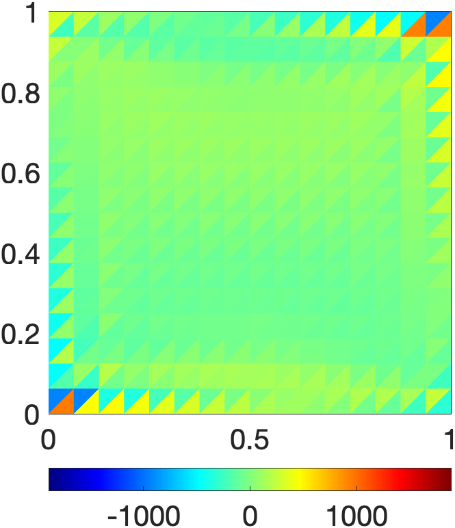
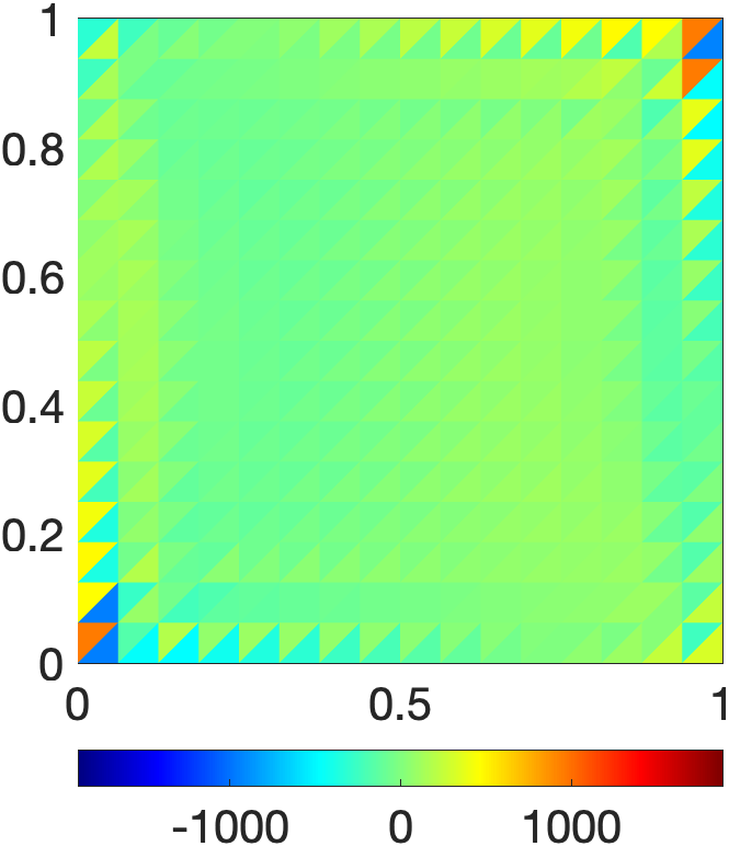
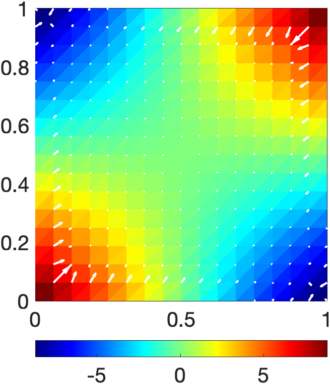
(a) ST-EG: $u_{1}$, $u_{2}$, and $p$ with the velocity vector fields, from left to right

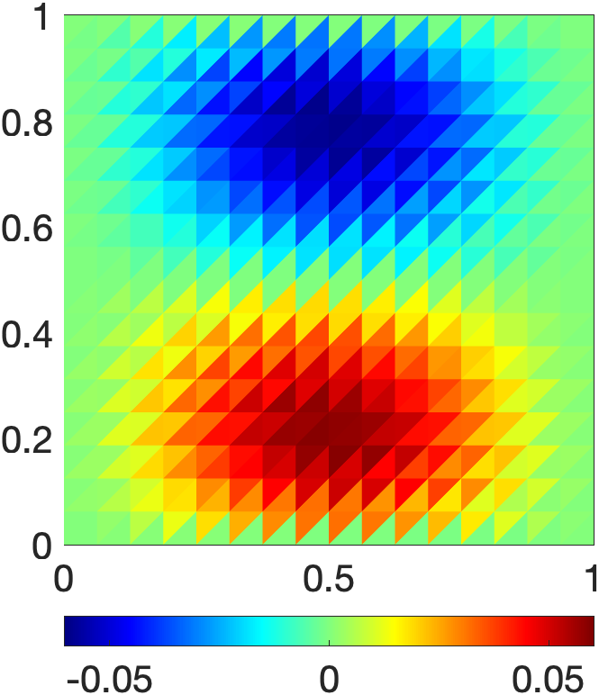
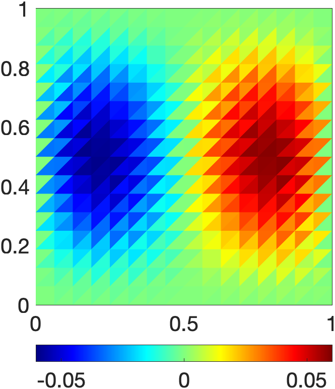
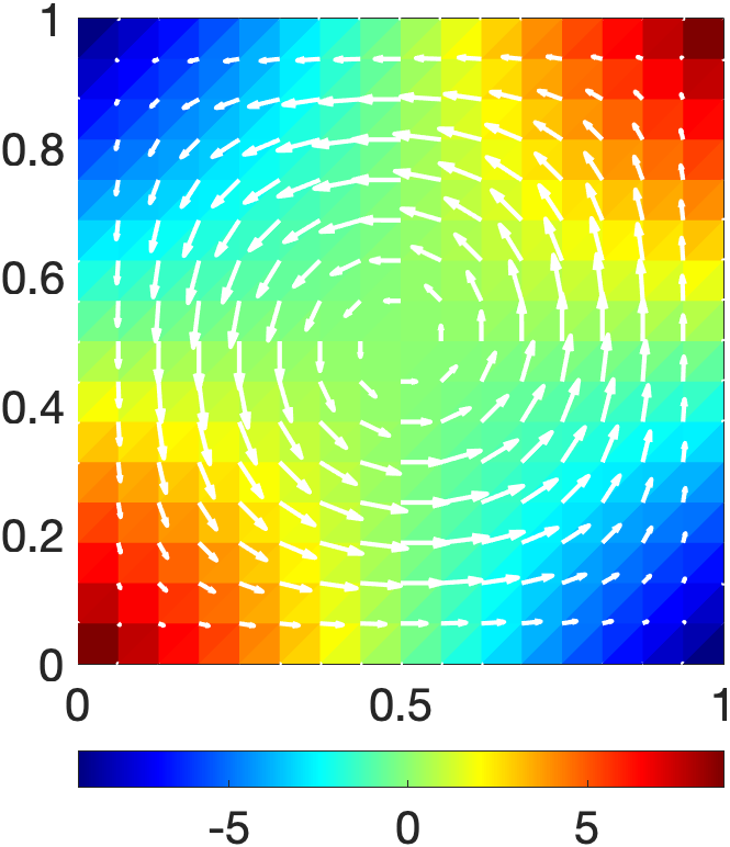
(b) PR-EG: $u_{1}$, $u_{2}$, and $p$ with the velocity vector fields, from left to right

Figure 1: Test 6.1.1, Vortex flow: Comparison of the numerical solutions with $h=1/16$ and $\nu=10^{-6}$.

Robustness test. This test is to verify the pressure-robustness of the PR-EG method. To confirm the error behaviors predicted by (6.1) and (6.2), we solved the example problem with varying $\nu$ values, from $10^{-2}$ to $10^{-6}$, while fixing the mesh size to $h=1/32$. Figure 2 shows the total velocity and auxiliary pressure errors, i.e., $\lVert{\bf u}-{\bf u}_{h}\rVert_{\mathcal{E}}$ and $\lVert\mathcal{P}_{0}p-p_{h}\rVert_{0}$. As expected, the ST-EG method produces the velocity errors inversely proportional to $\nu$ as the second term in the error bound (6.1a) becomes a dominant one as $\nu$ gets smaller. Meanwhile, the auxiliary pressure error remains nearly the same while $\nu$ varies. On the other hand, the PR-EG method produces nearly the same velocity errors regardless of the $\nu$ values. Moreover, the auxiliary pressure errors decrease in proportion to $\nu$. These numerical results are consistent with the error bounds (6.1) and (6.2).

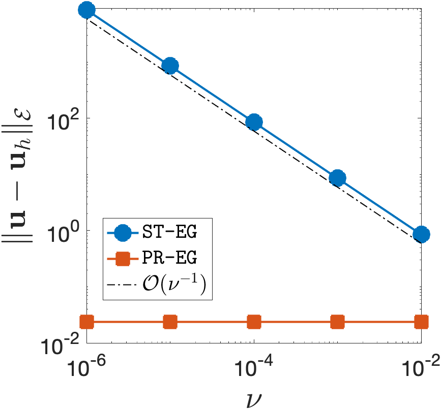
(a) Velocity error vs. viscosity

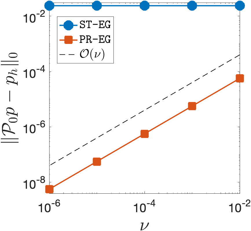
(b) Auxiliary pressure error vs. viscosity

Figure 2: Test 6.1.1, Vortex flow: Error profiles of the ST-EG and PR-EG methods with varying $\nu$ values and a fixed mesh size $h=1/32$.

Performance of the CPR-EG method. In this test, we shall validate the error estimates in Theorem 5.3 for the CPR-EG method and compare its performances with the PR-EG method. First, we consider the sparsity pattern of their stiffness matrices when generated on the same mesh of size $h=1/32$. Figure 3 compares the sparsity patterns of the stiffness matrices corresponding to PR-EG, PPR-EG, and CPR-EG methods. The PPR-EG method produces a matrix with less nonzero entries than the PR-EG method. It also shows the CPR-EG method yields a much smaller but denser stiffness matrix than the PR-EG method. More specifically, by eliminating the DG component of the velocity vector, we can achieve 33% reduction in the number of DoFs. To compare the accuracy of the two methods, we performed a numerical convergence study with varying $h$ values and a fixed viscosity $\nu=10^{-6}$, whose results are plotted in Figure 4. As observed in this figure, the errors produced by the CPR-EG method not only decrease at the optimal order of $\mathcal{O}(h)$, they are also nearly identical to those produced by the PR-EG method.

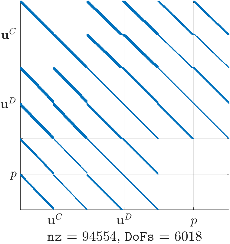
(a) PR-EG

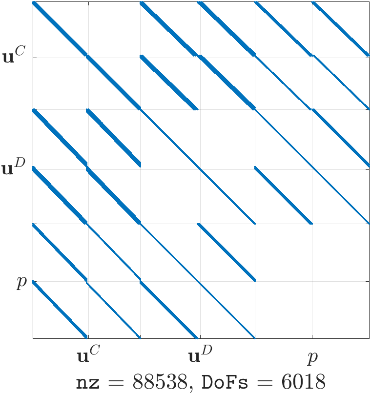
(b) PPR-EG

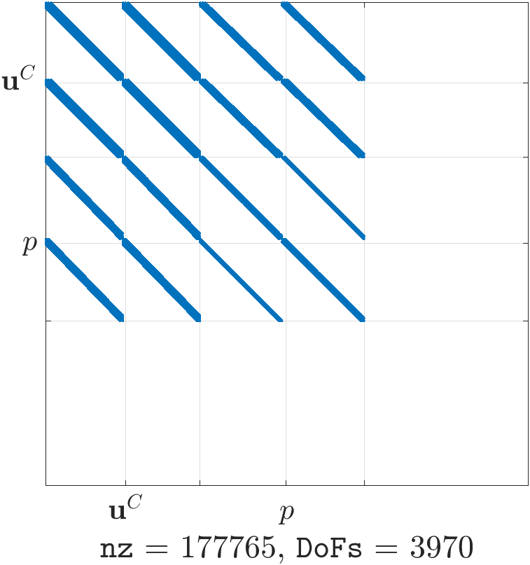
(c) CPR-EG

Figure 3: Test 6.1.1, Vortex flow: Comparison of the sparsity patterns of the stiffness matrices on a mesh with $h=1/32$. nz denotes the number of nonzeros.

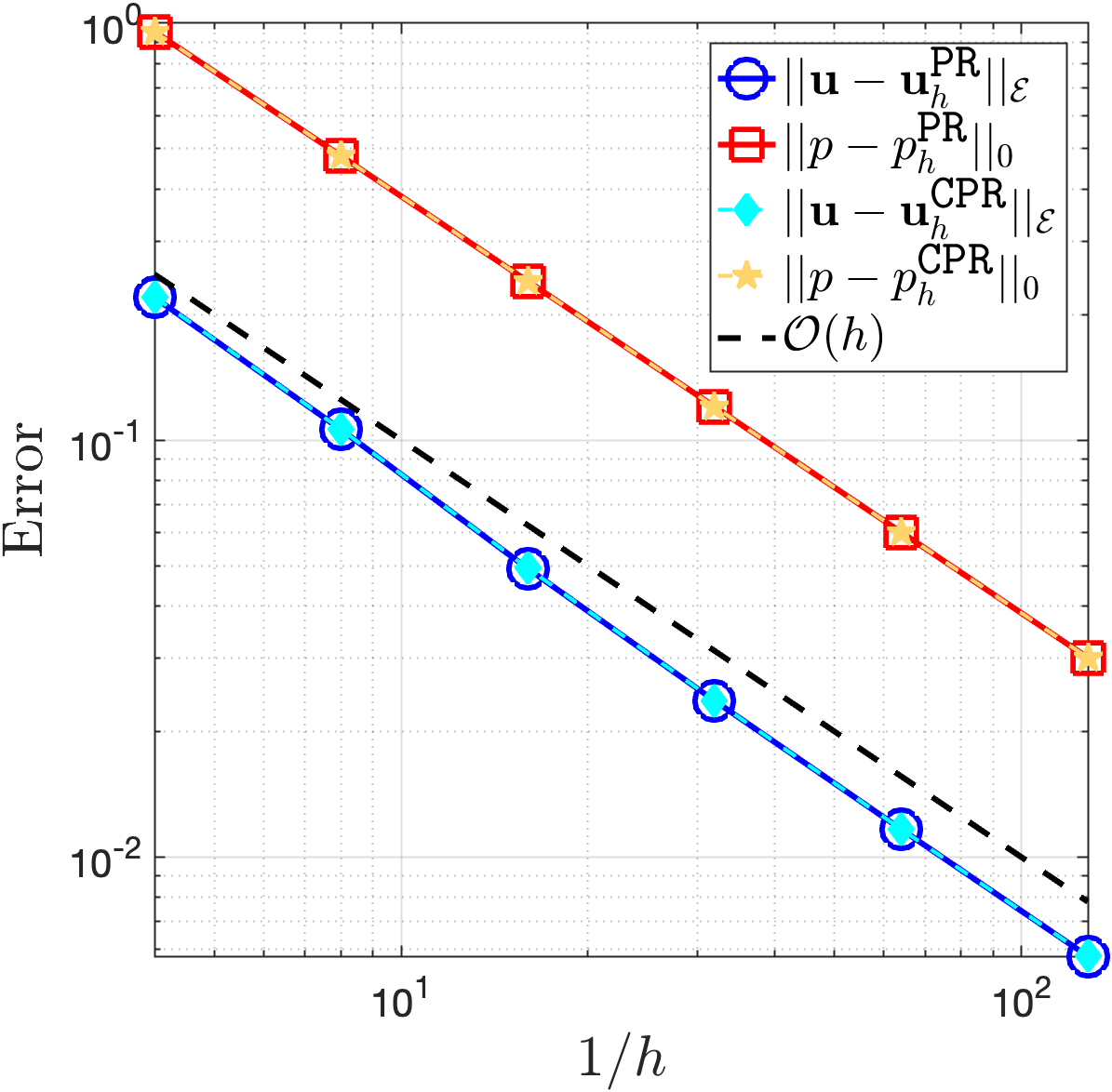
Figure 4: Test 6.1.1, Vortex flow: Comparison of the errors from the PR-EG and CPR-EG methods. The viscosity is fixed to $\nu=10^{-6}$.

6.2 Three dimensional examples

We now turn our attention to some numerical examples in three dimensions. In all three-dimensional tests, we used the penalty parameter $\rho=2$.

6.2.1 Test 2: 3D flow in a unit cube

In this example, we consider a 3D flow in a unit cube $\Omega=(0,1)^{3}$. The velocity field and pressure are chosen as

$${\bf u}=\left(\begin{array}[]{c}\sin(\pi x)\cos(\pi y)-\sin(\pi x)\cos(\pi z)\\ \sin(\pi y)\cos(\pi z)-\sin(\pi y)\cos(\pi x)\\ \sin(\pi z)\cos(\pi x)-\sin(\pi z)\cos(\pi y)\end{array}\right),\quad p=\sin(\pi x)\sin(\pi y)\sin(\pi z).$$

Accuracy test. With this example problem, we performed a mesh refinement study for the ST-EG and PR-EG methods with a fixed viscosity $\nu=10^{-6}$. The results, summarized in Table 2, show very similar convergence behaviors to those of the two-dimensional results. Though the velocity errors generated by the ST-EG method appear to decrease super-linearly, the magnitudes of the numerical velocity solutions are extremely larger than those of the exact solution and the solution of the PR-EG method. See the streamlines of the velocity solutions of the ST-EG and PR-EG methods in Figure 5.

	ST-EG				PR-EG
$h$	$\lVert{\bf u}-{\bf u}_{h}^{\texttt{ST}}\rVert_{\mathcal{E}}$	Rate	$\|p-p_{h}^{\texttt{ST}}\|_{0}$	Rate	$\|{\bf u}-{\bf u}_{h}^{\texttt{PR}}\|_{\mathcal{E}}$	Rate	$\|p-p_{h}^{\texttt{PR}}\|_{0}$	Rate
$1/4$	8.785e+3	-	1.058e-1	-	3.732e+0	-	9.581e-2	-
$1/8$	3.429e+3	1.36	5.144e-2	1.04	1.827e+0	1.03	4.879e-2	0.97
$1/16$	1.239e+3	1.47	2.514e-2	1.03	9.048e-1	1.01	2.451e-2	0.99
$1/32$	4.346e+2	1.51	1.241e-2	1.02	4.501e-1	1.01	1.227e-2	1.00
$1/64$	1.521e+2	1.51	6.171e-3	1.01	2.244e-1	1.00	6.135e-3	1.00

Table 2: Test 6.2.1, 3D flow in a unit cube: A mesh refinement study for the ST-EG and PR-EG methods on uniform meshes with varying $h$ and a fixed viscosity $\nu=10^{-6}$.

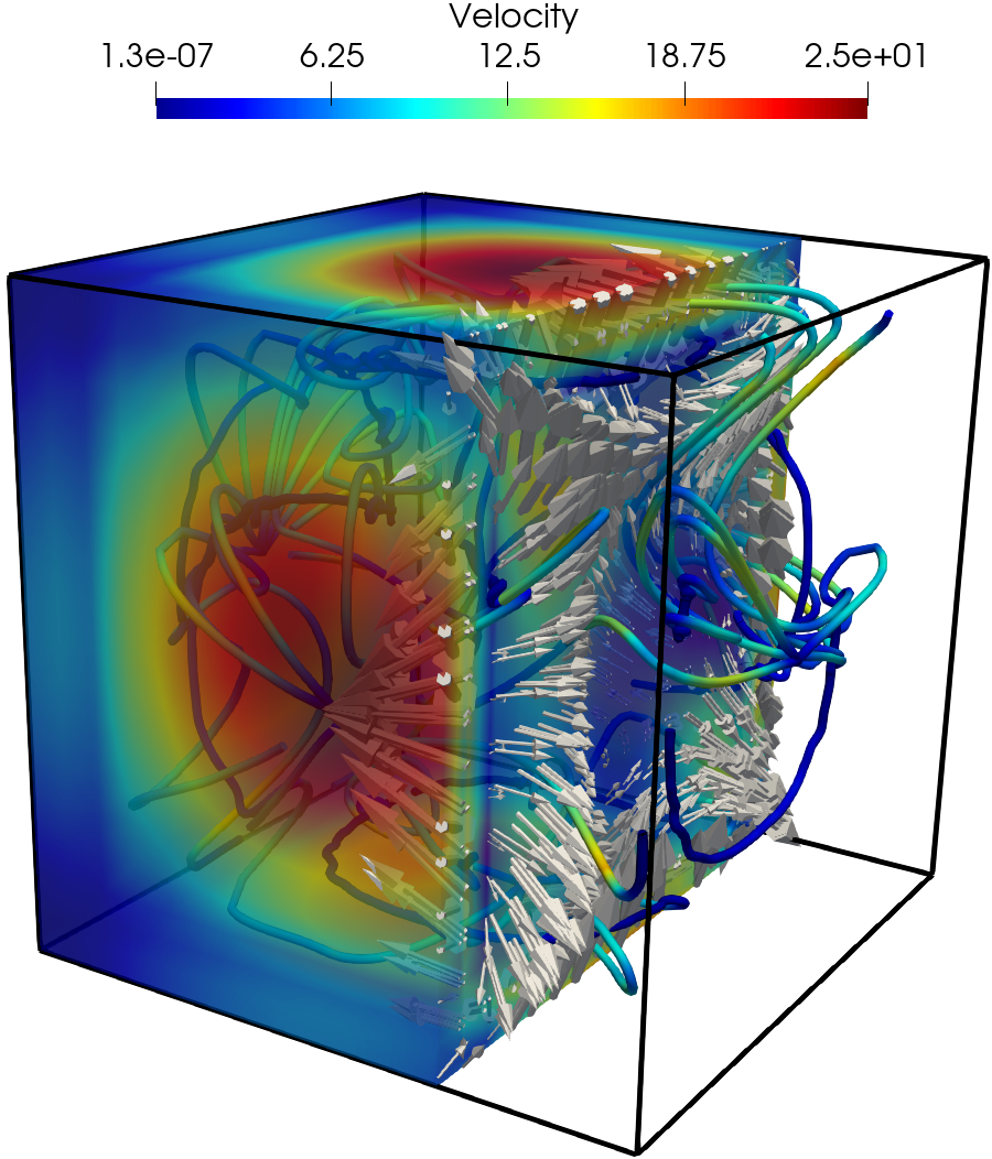
(a) ST-EG

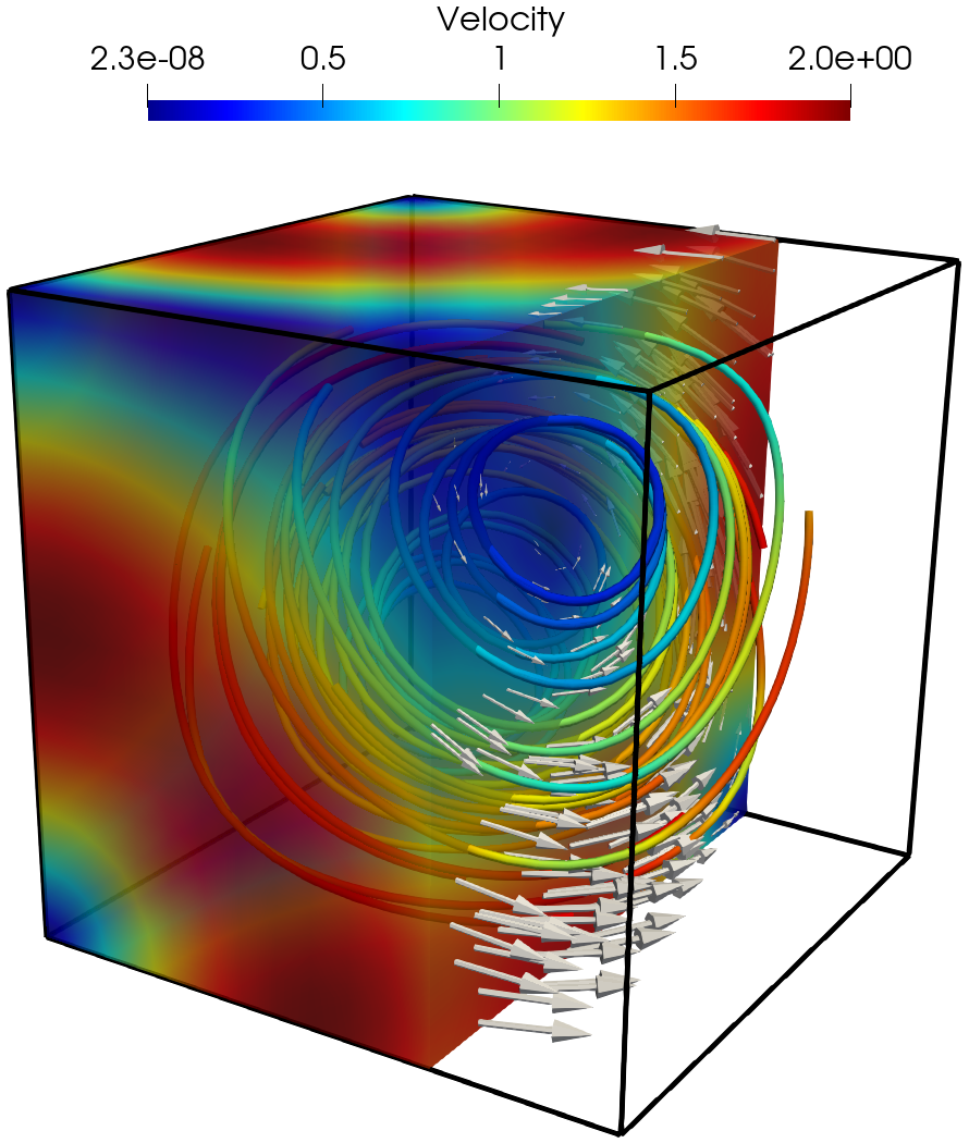
(b) PR-EG

Figure 5: Test 6.2.1, 3D flow in a unit cube: Streamlines of the numerical velocity when $h=1/16$ and $\nu=10^{-6}$.

Robustness test. We consider the pattern of the error behaviors obtained by the two EG methods when $\nu$ varies and the mesh size is fixed to $h=1/16$. The results of our tests are illustrated in Figure 6. As in the two-dimensional example, the velocity and (auxiliary) pressure errors for the PR-EG method follow the patterns predicted by the error estimates in (6.2). On the other hand, the velocity and auxiliary pressure errors for the ST-EG method behave like $\mathcal{O}(\nu^{-1})$ and $\mathcal{O}(1)$ only after $\nu$ becomes sufficiently small ($\nu\leq 10^{-3}$). The earlier deviation from these patterns when $\nu$ is relatively large ($10^{-3}\leq\nu\leq 10^{-2}$) is due to the smallness of $\lVert p\rVert_{1}$ compared to $\lVert{\bf u}\rVert_{2}$, unlike in Test 1.

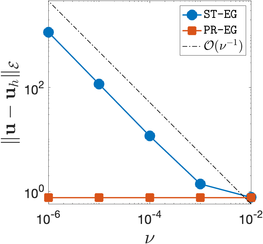
(a) Velocity error vs. viscosity

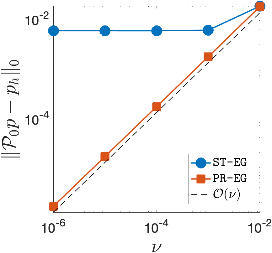
(b) Auxiliary pressure error vs. viscosity

Figure 6: Test 6.2.1, 3D flow in a unit cube: Error profiles of the ST-EG and PR-EG methods with varying $\nu$ and a fixed mesh size $h=1/16$.

Performance of the CPR-EG method. Next, we shall demonstrate the savings in the computational cost when we use the CPR-EG method. See Figure 7 for the sparsity patterns for the stiffness matrices generated by the PR-EG, PPR-EG, and CPR-EG methods on the same mesh with $h=1/16$. In this case, the PPR-EG method generates a stiffness matrix with fewer nonzero entries compared to the PR-EG method. On the other hand, the CPR-EG method requires approximately 38% fewer DoFs than the other two methods. However, its resulting stiffness matrix is denser than those resulting from the other two methods. Besides, we also compared the errors generated by the PR-EG and PPR-EG methods. They are nearly the same. But, the numerical data is not provided here for the sake of brevity.

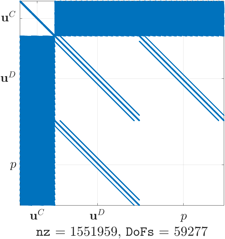
(a) PR-EG

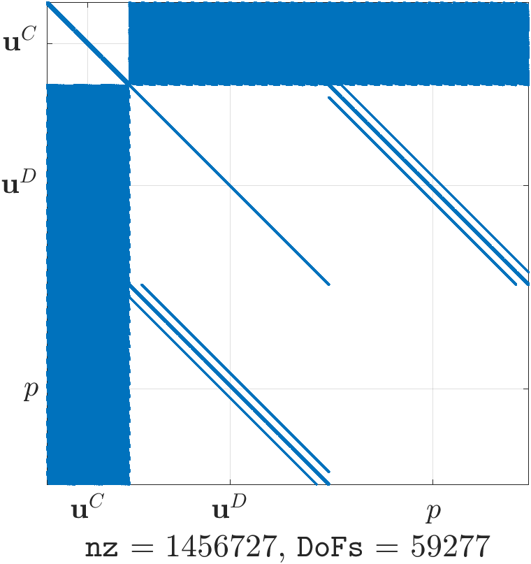
(b) PPR-EG

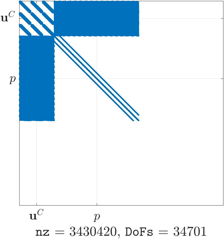
(c) CPR-EG

Figure 7: Test 6.2.1, 3D flow in a unit cube: Comparison of the sparsity patterns of the stiffness matrices on a mesh with $h=1/16$.

Performance of block preconditioners. We use the proposed block preconditioners to solve the corresponding linear systems and show their robustness with respect to the viscosity $\nu$. The required iteration numbers are reported in Table 3 for mesh size $h=1/4$ and penalty parameter $\rho=2$. The exact and inexact block preconditioners are applied to the preconditioned GMRES method. For the inexact block preconditioners, we use an algebraic multigrid (AMG) preconditioned GMRES method to approximately invert the diagonal block with tolerance $10^{-6}$. This inner block solver usually took $5$-$7$ iterations in all our experiments. Therefore, we only report the outer GMRES iteration numbers. The results in Table 3 show the robustness of our block preconditioners with respect to the viscosity $\nu$. This is further confirmed in Table 4, where the condition numbers of the preconditioned stiffness matrices are reported. In Table 4, we only show the results of the application of the block diagonal preconditioner since, in this case, the preconditioner is symmetric positive definite and the condition number is defined via the eigenvalues, i.e., $\kappa(\mathcal{B}_{D}\mathcal{A})=\frac{\max|\lambda(\mathcal{B}_{D}\mathcal{A})|}{\min|\lambda(\mathcal{B}_{D}\mathcal{A})|}$, $\kappa(\mathcal{B}^{D}_{D}\mathcal{A}^{D})=\frac{\max|\lambda(\mathcal{B}^{D}_{D}\mathcal{A}^{D})|}{\min|\lambda(\mathcal{B}^{D}_{D}\mathcal{A}^{D})|}$, and $\kappa(\mathcal{B}^{E}_{D}\mathcal{A}^{E})=\frac{\max|\lambda(\mathcal{B}^{E}_{D}\mathcal{A}^{E})|}{\min|\lambda(\mathcal{B}^{E}_{D}\mathcal{A}^{E})|}$. As we can see, the condition number remains the same as $\nu$ decreases, which demonstrates the robustness of the proposed block preconditioners. The small variation in the number of iterations is mainly due to the outer GMRES method since the matrices $\mathcal{A}$, $\mathcal{A}^{D}$, and $\mathcal{A}^{E}$ are ill-conditioned and may affect the orthogonalization procedure used in Krylov iterative methods. In addition, the numerical performance for the CPR-EG method is the best among all three pressure-robust methods for this test in terms of the number of iterations.

	Exact Solver
	PR-EG			PPR-EG			CPR-EG
$\nu$	$\mathcal{B}_{D}$	$\mathcal{B}_{L}$	$\mathcal{B}_{U}$	$\mathcal{B}^{D}_{D}$	$\mathcal{B}^{D}_{L}$	$\mathcal{B}^{D}_{U}$	$\mathcal{B}^{E}_{D}$	$\mathcal{B}^{E}_{L}$	$\mathcal{B}^{E}_{U}$
1	43	23	21	62	34	32	30	20	18
$10^{-2}$	61	33	33	87	49	49	45	27	28
$10^{-4}$	71	39	39	89	52	52	39	25	25
$10^{-6}$	72	40	40	91	55	55	36	25	25
	Inexact Solver
	PR-EG			PPR-EG			CPR-EG
$\nu$	$\mathcal{M}_{D}$	$\mathcal{M}_{L}$	$\mathcal{M}_{U}$	$\mathcal{M}^{D}_{D}$	$\mathcal{M}^{D}_{L}$	$\mathcal{M}^{D}_{U}$	$\mathcal{M}^{E}_{D}$	$\mathcal{M}^{E}_{L}$	$\mathcal{M}^{E}_{U}$
1	43	27	25	63	37	34	34	21	19
$10^{-2}$	61	36	35	93	56	56	53	30	31
$10^{-4}$	75	45	45	96	61	61	47	29	28
$10^{-6}$	83	47	47	111	64	64	40	28	27

Table 3: Test 6.2.1, 3D flow in a unit cube: Iteration counts for the block preconditioners when $\nu$ varies on mesh with $h=1/4$.

	PR-EG	PPR-EG	CPR-EG
$\nu$	$\kappa(\mathcal{B}_{D}\mathcal{A})$	$\kappa(\mathcal{B}^{D}_{D}\mathcal{A}^{D})$	$\kappa(\mathcal{B}^{E}_{D}\mathcal{A}^{E})$
1	41.267	99.563	62.445
$10^{-2}$	41.267	99.563	62.445
$10^{-4}$	41.267	99.563	62.445
$10^{-6}$	41.267	99.563	62.445

Table 4: Test 6.2.1, 3D flow in a unit cube: Condition number of the preconditioned stiffness matrices with the exact block preconditioners when $\nu$ varies on mesh with $h=1/4$.

6.2.2 Test 3: 3D vortex flow in L-shaped cylinder

Let us consider an L-shaped cylinder defined by $\Omega=(0,1)^{3}\setminus(0.5,1)\times(0.5,1)\times(0,1)$. In this domain, the exact velocity field and pressure are chosen as

$${\bf u}=\frac{1}{x^{2}+y^{2}+1}\left(\begin{array}[]{c}-y\\ x\\ 0\end{array}\right),\quad p=|2x-1|.$$

Note that the velocity is a rotational vector field whose center is $(x,y)=(0,0)$, and the pressure contains discontinuity in its derivatives along the vertical line $x=0.5$.

Accuracy and robustness test. We performed a mesh refinement study with $\nu=10^{-6}$ and also studied the error behaviors on a fixed mesh while $\nu$ varies for both the ST-EG and PR-EG methods. The error behaviors are very similar to those of the previous examples reported in, for example, Table 2 and Figure 6. Therefore, we omit the results here. However, we present the streamlines of the numerical velocity solutions in Figure 8. The side-by-side comparison of the velocity streamlines generated by the ST-EG and PR-EG methods clearly shows that the PR-EG method well captures the characteristic of the rotational vector field while the ST-EG method does not.

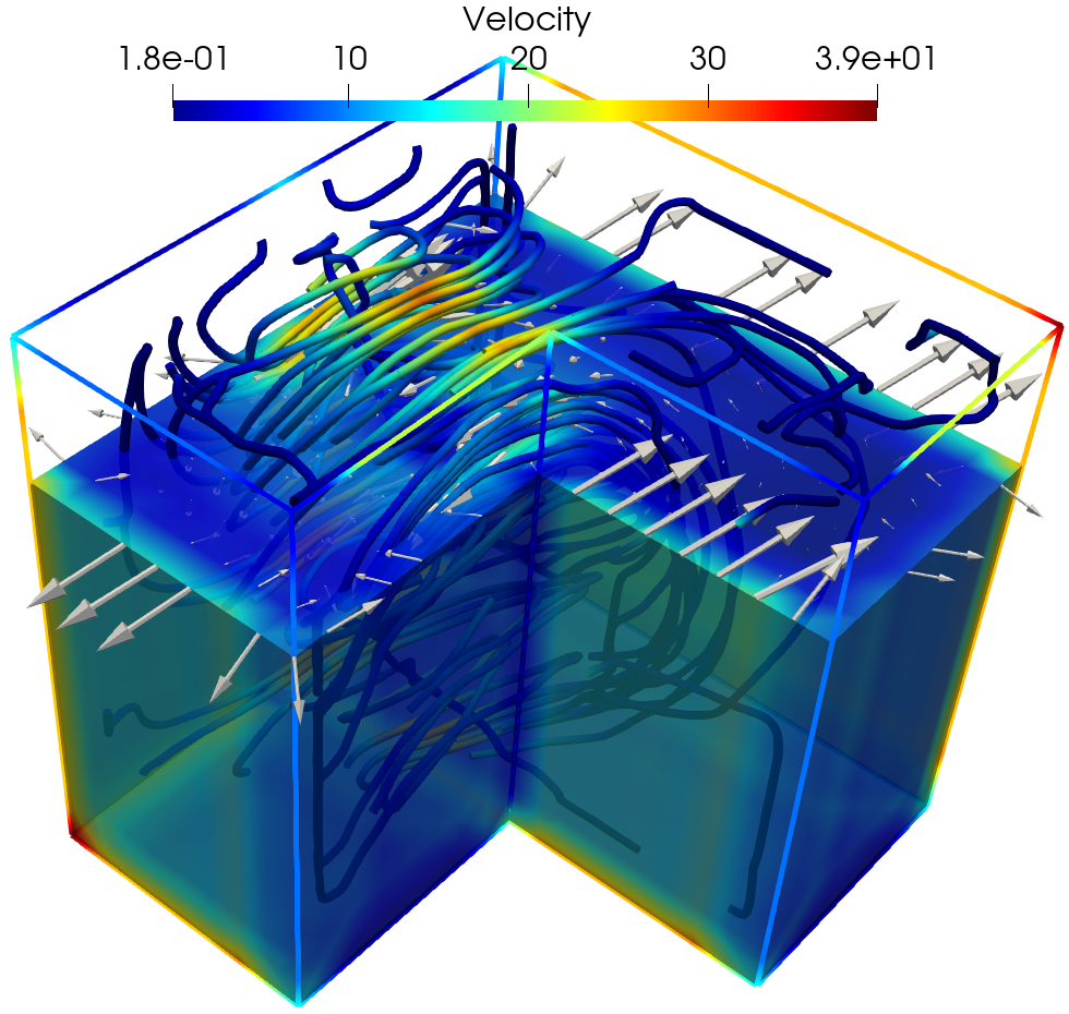
(a) ST-EG

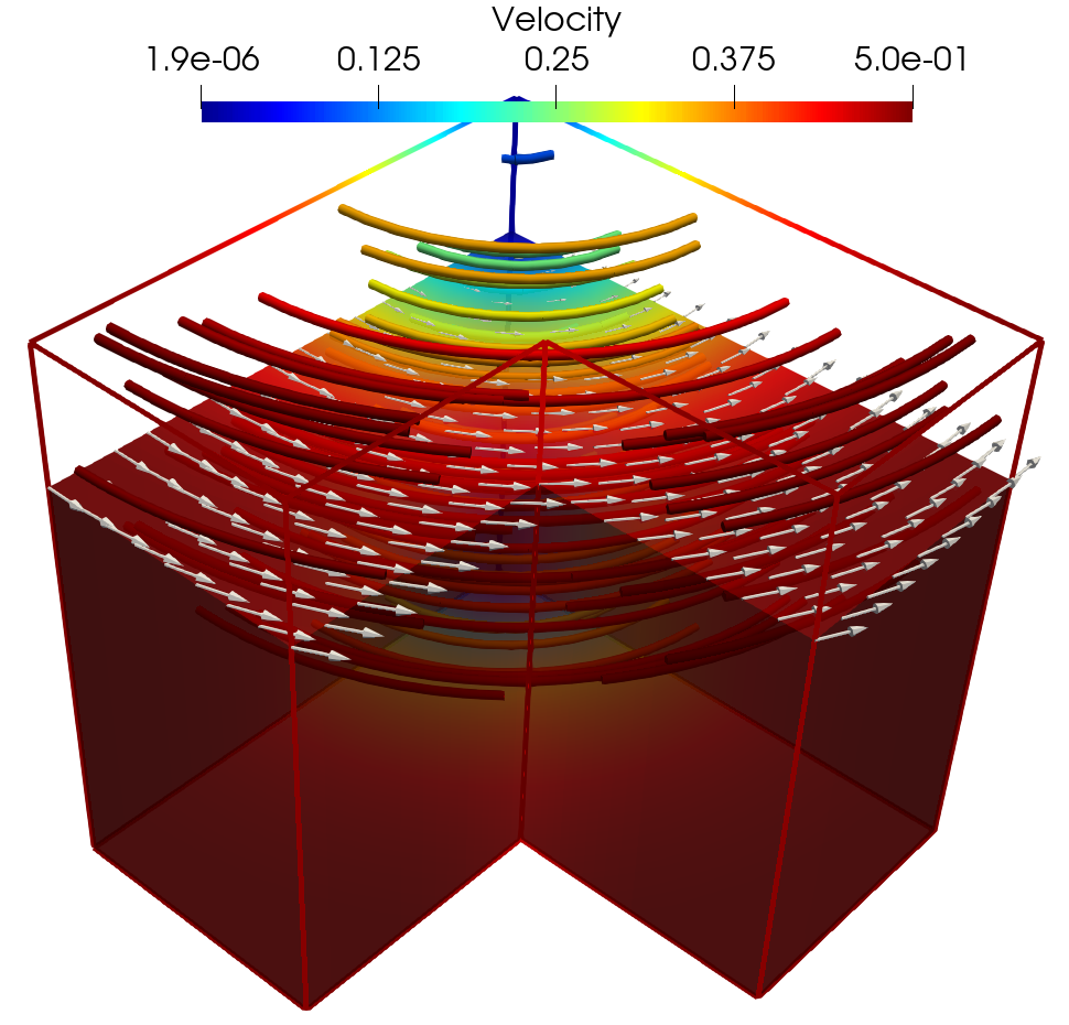
(b) PR-EG

Figure 8: Test 6.2.2, 3D Vortex flow in an L-shaped cylinder: Streamlines of the numerical velocity solutions with $h=1/16$ and $\nu=10^{-6}$.

Performance of block preconditioners. We again test the performance of the block preconditioners for this 3D L-shaped domain example. The block preconditioners were implemented in the same way as in Test 6.2.1. The inner GMRES method for solving the diagonal blocks usually took $6$-$9$ iterations in all cases, hence the results are omitted here, but the numbers of iterations of the outer GMRES method are shown in Table 5. When the block preconditioners are used for the PR-EG and PPR-EG methods, the numbers of iterations increase moderately as the viscosity $\nu$ decreases. This is mainly caused by the outer GMRES method since the condition numbers of the preconditioned stiffness matrices remain constant when $\nu$ decreases, as shown in Table 6. Interestingly, the CPR-EG method performs the best in terms of the number of iterations. However, its condition number is slightly larger than that of the PR-EG method, as shown in Table 6. Further studies are needed to better understand those observations to design parameter-robust preconditioners that can be applied in practice. But this is out of the scope of this work and will be part of our future research.

	Exact Solver
	PR-EG			PPR-EG			CPR-EG
$\nu$	$\mathcal{B}_{D}$	$\mathcal{B}_{L}$	$\mathcal{B}_{U}$	$\mathcal{B}^{D}_{D}$	$\mathcal{B}^{D}_{L}$	$\mathcal{B}^{D}_{U}$	$\mathcal{B}^{E}_{D}$	$\mathcal{B}^{E}_{L}$	$\mathcal{B}^{E}_{U}$
1	98	50	49	116	62	59	64	33	31
$10^{-2}$	161	85	85	207	113	113	102	56	56
$10^{-4}$	189	101	101	252	136	136	105	57	57
$10^{-6}$	217	120	120	–	161	161	105	57	57
	Inexact Solver
	PR-EG			PPR-EG			CPR-EG
$\nu$	$\mathcal{M}_{D}$	$\mathcal{M}_{L}$	$\mathcal{M}_{U}$	$\mathcal{M}^{D}_{D}$	$\mathcal{M}^{D}_{L}$	$\mathcal{M}^{D}_{U}$	$\mathcal{M}^{E}_{D}$	$\mathcal{M}^{E}_{L}$	$\mathcal{M}^{E}_{U}$
1	98	54	55	116	67	65	64	36	34
$10^{-2}$	161	92	92	207	121	121	102	61	61
$10^{-4}$	189	112	112	251	147	147	105	63	62
$10^{-6}$	211	127	127	279	170	168	105	63	62

Table 5: Test 6.2.2, 3D flow in L-shaped domain: Iteration counts for the block preconditioners when $\nu$ varies on mesh with $h=1/4$.

	PR-EG	PPR-EG	CPR-EG
$\nu$	$\kappa(\mathcal{B}_{D}\mathcal{A})$	$\kappa(\mathcal{B}^{D}_{D}\mathcal{A}^{D})$	$\kappa(\mathcal{B}^{E}_{D}\mathcal{A}^{E})$
1	130.450	267.947	164.076
$10^{-2}$	130.450	267.947	164.076
$10^{-4}$	130.450	267.947	164.076
$10^{-4}$	130.450	267.947	164.076

Table 6: Test 6.2.2, 3D flow in L-shaped domain: Condition number of the preconditioned stiffness matrices with the exact block preconditioners when $\nu$ varies on mesh with $h=1/4$.

7 Conclusions

In this paper, we proposed a pressure-robust EG scheme for solving the Stokes equations, describing the steady-state, incompressible viscous fluid flow. The new EG method is based on the recent work [42] on a stable EG scheme for the Stokes problem, where the velocity error depends on the pressure error and is inversely proportional to viscosity. In order to make the EG scheme in [42] a pressure-robust scheme, we employed a velocity reconstruction operator on the load vector on the right-hand side of the discrete system. Despite this simple modification, our error analysis shows that the velocity error of the new EG scheme is independent of viscosity and the pressure error, and the method maintains the optimal convergence rates for both the velocity and pressure. We also considered a perturbed version of our pressure-robust EG method. This perturbed method allows for the elimination of the DoFs corresponding to the DG component of the velocity vector via static condensation. The resulting condensed linear system can be viewed as an $H^{1}$-conforming $\mathbb{P}_{1}$-$\mathbb{P}_{0}$ scheme with stabilization terms. This stabilized $\mathbb{P}_{1}$-$\mathbb{P}_{0}$ scheme is inf-sup stable and pressure-robust as well. Furthermore, we proposed an efficient preconditioning technique whose performance is robust with respect to viscosity. Our two- and three-dimensional numerical experiments verified the theoretical results. In the future, this work will be extended to more complicated incompressible flow models, such as the Oseen and Navier-Stokes equations, where the pressure-robustness is important for simulations in various flow regimes.

Acknowlegements

The work of Son-Young Yi was supported by the U.S. National Science Foundation grant DMS-2208426.

References

• Adler et al. [2017] James H Adler, Francisco J Gaspar, Xiaozhe Hu, Carmen Rodrigo, and Ludmil T Zikatanov. Robust block preconditioners for Biot’s model. In International Conference on Domain Decomposition Methods, pages 3–16. Springer, 2017.
• Adler et al. [2020] James H Adler, Francisco José Gaspar, Xiaozhe Hu, Peter Ohm, Carmen Rodrigo, and Ludmil T Zikatanov. Robust preconditioners for a new stabilized discretization of the poroelastic equations. SIAM Journal on Scientific Computing, 42(3):B761–B791, 2020.
• Arnold and Qin [1992] Douglas N Arnold and Jinshui Qin. Quadratic velocity/linear pressure Stokes elements. Advances in Computer Methods for Partial Differential Equations, 7:28–34, 1992.
• Babuška [1973] Ivo Babuška. The finite element method with Lagrangian multipliers. Numerische Mathematik, 20(3):179–192, 1973.
• Bernardi and Raugel [1985] Christine Bernardi and Genevieve Raugel. Analysis of some finite elements for the Stokes problem. Mathematics of Computation, 44(169):71–79, 1985.
• Brezzi [1974] Franco Brezzi. On the existence, uniqueness and approximation of saddle-point problems arising from Lagrangian multipliers. Publications mathématiques et informatique de Rennes, (S4):1–26, 1974.
• Brezzi and Fortin [1991] Franco Brezzi and Michel Fortin. Mixed and Hybrid Finite Element Methods, volume 15 of Springer Series in Computational Mathematics. Springer-Verlag, New York, 1991. isbn:0-387-97582-9.
• Chaabane et al. [2018] Nabil Chaabane, Vivette Girault, Beatrice Riviere, and Travis Thompson. A stable enriched Galerkin element for the Stokes problem. Applied Numerical Mathematics, 132:1--21, 2018.
• Chen [2009] Long Chen. iFEM: An Integrated Finite Element Methods Package in MATLAB. Technical Report, University of California at Irvine, 2009.
• Chen and Wang [2019] Long Chen and Feng Wang. A divergence free weak virtual element method for the Stokes problem on polytopal meshes. Journal of Scientific Computing, 78(2):864--886, 2019.
• Chen et al. [2015] Long Chen, Ming Wang, and Lin Zhong. Convergence analysis of triangular MAC schemes for two dimensional Stokes equations. Journal of Scientific Computing, 63(3):716--744, 2015.
• Cockburn et al. [2007] Bernardo Cockburn, Guido Kanschat, and Dominik Schötzau. A note on discontinuous Galerkin divergence-free solutions of the Navier--Stokes equations. Journal of Scientific Computing, 31(1):61--73, 2007.
• Crouzeix and Raviart [1973] Michel Crouzeix and P-A Raviart. Conforming and nonconforming finite element methods for solving the stationary Stokes equations I. Revue française d’automatique informatique recherche opérationnelle. Mathématique, 7(R3):33--75, 1973.
• Falk and Neilan [2013] Richard S Falk and Michael Neilan. Stokes complexes and the construction of stable finite elements with pointwise mass conservation. SIAM Journal on Numerical Analysis, 51(2):1308--1326, 2013.
• Gauger et al. [2019] Nicolas R Gauger, Alexander Linke, and Philipp W Schroeder. On high-order pressure-robust space discretisations, their advantages for incompressible high Reynolds number generalised Beltrami flows and beyond. The SMAI Journal of Computational Mathematics, 5:89--129, 2019.
• Girault and Raviart [1986] Vivette Girault and Pierre-Arnaud Raviart. Finite Element Methods for Navier-Stokes Equations, volume 5 of Springer Series in Computational Mathematics. Springer-Verlag, Berlin, 1986. isbn:3-540-15796-4. Theory and algorithms.
• Girault et al. [2005] Vivette Girault, Béatrice Rivière, and Mary Wheeler. A discontinuous Galerkin method with nonoverlapping domain decomposition for the Stokes and Navier-Stokes problems. Mathematics of Computation, 74(249):53--84, 2005.
• Guzmán and Neilan [2014a] Johnny Guzmán and Michael Neilan. Conforming and divergence-free Stokes elements on general triangular meshes. Mathematics of Computation, 83(285):15--36, 2014a.
• Guzmán and Neilan [2014b] Johnny Guzmán and Michael Neilan. Conforming and divergence-free Stokes elements in three dimensions. IMA Journal of Numerical Analysis, 34(4):1489--1508, 2014b.
• Hansbo and Larson [2008] Peter Hansbo and Mats G Larson. Piecewise divergence-free discontinuous Galerkin methods for Stokes flow. Communications in Numerical Methods in Engineering, 24(5):355--366, 2008.
• Jenkins et al. [2014] Eleanor W Jenkins, Volker John, Alexander Linke, and Leo G Rebholz. On the parameter choice in grad-div stabilization for the Stokes equations. Advances in Computational Mathematics, 40(2):491--516, 2014.
• Ladyzhenskaya [1969] Olga Aleksandrovna Ladyzhenskaya. The Mathematical Theory of Viscous Incompressible Flow, volume 2. Gordon and Breach New York, 1969.
• Li and Zikatanov [2022] Yuwen Li and Ludmil T. Zikatanov. New stabilized ${P}_{1}\times{P}_{0}$ finite element methods for nearly inviscid and incompressible flows. Computer Methods in Applied Mechanics and Engineering, 393:114815, apr 2022.
• Linke [2012] Alexander Linke. A divergence-free velocity reconstruction for incompressible flows. Comptes Rendus Mathematique, 350(17-18):837--840, 2012.
• Linke [2014] Alexander Linke. On the role of the Helmholtz decomposition in mixed methods for incompressible flows and a new variational crime. Computer Methods in Applied Mechanics and Engineering, 268:782--800, 2014.
• Linke and Merdon [2016] Alexander Linke and Christian Merdon. Pressure-robustness and discrete Helmholtz projectors in mixed finite element methods for the incompressible Navier--Stokes equations. Computer Methods in Applied Mechanics and Engineering, 311:304--326, 2016.
• Loghin and Wathen [2004] Daniel Loghin and Andrew J Wathen. Analysis of preconditioners for saddle-point problems. SIAM Journal on Scientific Computing, 25(6):2029--2049, 2004.
• Mardal and Winther [2011] Kent-Andre Mardal and Ragnar Winther. Preconditioning discretizations of systems of partial differential equations. Numerical Linear Algebra with Applications, 18(1):1--40, 2011.
• Mu [2020] Lin Mu. Pressure robust weak Galerkin finite element methods for Stokes problems. SIAM Journal on Scientific Computing, 42(3):B608--B629, 2020.
• Mu et al. [2018] Lin Mu, Junping Wang, Xiu Ye, and Shangyou Zhang. A discrete divergence free weak Galerkin finite element method for the Stokes equations. Applied Numerical Mathematics, 125:172--182, 2018.
• Mu et al. [2021a] Lin Mu, Xiu Ye, and Shangyou Zhang. A stabilizer-free, pressure-robust, and superconvergence weak Galerkin finite element method for the Stokes equations on polytopal mesh. SIAM Journal on Scientific Computing, 43(4):A2614--A2637, 2021a.
• Mu et al. [2021b] Lin Mu, Xiu Ye, and Shangyou Zhang. Development of pressure-robust discontinuous Galerkin finite element methods for the Stokes problem. Journal of Scientific Computing, 89(1):1--25, 2021b.
• Olshanskii and Reusken [2004] Maxim Olshanskii and Arnold Reusken. Grad-div stablilization for Stokes equations. Mathematics of Computation, 73(248):1699--1718, 2004.
• Raviart and Thomas [2006] Pierre Arnaud Raviart and Jean Marie Thomas. A mixed finite element method for 2-nd order elliptic problems. In Mathematical Aspects of Finite Element Methods: Proceedings of the Conference Held in Rome, December 10--12, 1975, pages 292--315. Springer, 2006.
• Roberts and Thomas [1991] J. E. Roberts and J.-M. Thomas. Mixed and hybrid methods. In Handbook of Numerical Analysis, Vol. II, pages 523--639. North-Holland, Amsterdam, 1991.
• Rodrigo et al. [2016] Carmen Rodrigo, F J Gaspar, Xiaozhe Hu, and L T Zikatanov. Stability and monotonicity for some discretizations of the Biot’s consolidation model. Computer Methods in Applied Mechanics and Engineering, 298:183--204, 2016.
• Rodrigo et al. [2018] Carmen Rodrigo, Xiaozhe Hu, Peter Ohm, James H Adler, Francisco J Gaspar, and L T Zikatanov. New stabilized discretizations for poroelasticity and the Stokes’ equations. Computer Methods in Applied Mechanics and Engineering, 341:467--484, 2018.
• Scott and Vogelius [1985] L Ridgway Scott and Michael Vogelius. Conforming finite element methods for incompressible and nearly incompressible continua. Lectures in Applied Mathematics, 22(2), 1985.
• Taylor and Hood [1973] Cedric Taylor and Paul Hood. A numerical solution of the Navier-Stokes equations using the finite element technique. Computers & Fluids, 1(1):73--100, 1973.
• Wang et al. [2021] Gang Wang, Lin Mu, Ying Wang, and Yinnian He. A pressure-robust virtual element method for the Stokes problem. Computer Methods in Applied Mechanics and Engineering, 382:113879, 2021.
• Wang and Ye [2007] Junping Wang and Xiu Ye. New finite element methods in computational fluid dynamics by H(div) elements. SIAM Journal on Numerical Analysis, 45(3):1269--1286, 2007.
• Yi et al. [2022a] Son-Young Yi, Xiaozhe Hu, Sanghyun Lee, and James H. Adler. An enriched Galerkin method for the Stokes equations. Computers and Mathematics with Applications, 120:115--131, 2022a.
• Yi et al. [2022b] Son-Young Yi, Sanghyun Lee, and Ludmil Zikatanov. Locking-free enriched Galerkin method for linear elasticity. SIAM Journal on Numerical Analysis, 60(1):52--75, 2022b. ISSN 0036-1429.