Modelling structural zeros in compositional data via a zero-censored multivariate normal model
Michail Tsagris

Department of Economics, University of Crete, Rethymnon, Greece, mtsagris@uoc.gr

Abstract

We present a new model for analyzing compositional data with structural zeros. Inspired by Butler and Glasbey (2008) who suggested a model in the presence of zero values in the data we propose a model that treats the zero values in a different manner. Instead of projecting every zero value towards a vertex, we project them onto their corresponding edge and fit a zero-censored multivariate model.

Keywords: compositional data, $\alpha$-transformation, structural zeros, zero-censoring

1 Introduction

Structural (and rounded) zeros are sometimes met in compositional data. The term structural refers to values which are truly zeros, for instance the percentage of money a family spends on smoking or alcohol. Rounded zeros on the other hand are very small values in some components which were rounded to zero. In geology for example the instrument which measures the composition of the elements has a detection limit. Values below that limit are not detected. This has two possible explanations; either the element is completely absent or had a value smaller than the detection limit of the instrument.

Ever since 1982 (Aitchison, 1982), the most widely used approach for compositional data analysis is the log-ratio approach. The nature of the logs though gives rise to a mathematical problem, the log of zero is undefined. This problem was dealt with simple imputation techniques such as imputation by a small value (Aitchison, 2003), or with substitution of the zero by a fraction of the detection limit (Palarea Albaladejo et al., 2005), or via the EM algorithm (Palarea-Albaladejo et al., 2007). If the zeros present are indeed rounded down only because the detection limit of the instrument was not that low, then these approaches can be used. However, even in this case, the true value could be lower than estimated. (Scealy and Welsh, 2011a) showed an example of the problem when these approaches are adopted. The smaller the imputed value is, the higher the magnitude of the log-ratio transformed values are. If on the other hand the value is a true zero (not rounded), then any imputation technique is clearly not correct.

(Butler and Glasbey, 2008) proposed a latent Gaussian model for modelling zero values. They used a multivariate normal distribution in $\mathbb{R}^{d}$ to model the data. When a point was outside the simplex they projected it orthogonally onto the faces and vertices of the simplex. However this approach has the problem of sometimes assigning too much probability on the vertices and sometimes more than is necessary. Furthermore, the higher the dimensionality of the simplex, finding the correct regions to project the points lying outside the simplex becomes more difficult. Maximum likelihood estimation becomes more difficult also, but with the use of MCMC methods they managed to tackle the estimation problems. We propose a different model for handling zero values, which is inspired though from that model (Butler and Glasbey, 2008). Instead of using an orthogonal projection for the points lying outside the simplex we move them along the line connecting the points with the center of the simplex.

In this section we will discuss the issue of structural zeros, that is when the value observed is actually zero and is not due to a rounding error. We will suggest a new method for modelling structural zeros based on the multivariate normal distribution. It is a different projection than the one suggested by Butler and Glasbey (2008). Since the simplex has the form of a triangle (when $D=3$), it seems that the projection of the points lying outside the simplex should be projected onto the boundaries of the simplex following a similar idea to the folded model (Tsagris and Stewart, 2020).

2 The $\alpha$-transformation

2.1 The stay-in-the-simplex version of the $\alpha$-transformation

The power transformation defined by Aitchison (2003) we saw earlier in Section LABEL:add is

$$\mathbf{u}=\{u_{i}\}_{i=1,\ldots,D}=\left\{\frac{x_{i}^{\alpha}}{\sum_{j=1}^{D}x_{j}^{\alpha}}\right\}_{i=1,\ldots,D}.$$ (1)

We shall call (1) the stay-in-the-simplex version of the $\alpha$-transformation. Note that the map (1) is degenerate due to the constraints $\sum_{i=1}^{D}x_{i}=1$ and $\sum_{i=1}^{D}u_{i}=1$. In order to make (1) non-degenerate we consider the version of (1) as follows

$$u_{i}\left\{\left(x_{j}\right)_{j=1}^{d}\right\}=\frac{x_{i}^{\alpha}}{\sum_{j=1}^{d}x_{j}^{\alpha}+\left(1-\sum_{j=1}^{d}x_{j}\right)^{\alpha}}\ \ \ i=1,\ldots,d.$$ (2)

The (2) is presented to highlight that in fact we have $d=D-1$ and not $D$ variables. Thus, the Jacobian of (1) or (2) is not singular. The Jacobian of the stay-in-the-simplex version of the $\alpha$-transformation (1) is equal to (Tsagris and Stewart, 2020)

$$\left|{\bf J}\right|=\alpha^{d}\prod_{i=1}^{D}\frac{x_{i}^{\alpha-1}}{\sum_{j=1}^{D}x_{j}^{\alpha}}.$$ (3)

2.2 The $\alpha$-transformation

A centred and scaled version of (1) is defined as

$$B_{\alpha}\left({\bf x}\right)={\bf H}\frac{1}{\alpha}\left(D{\bf u}-{\bf 1}_{D}\right),$$ (4)

where ${\bf u}$ is defined in (1), ${\bf 1}_{D}$ is the $D$-dimensional vector of $1$s and ${\bf H}$ is the Helmert sub-matrix (Tsagris et al., 2011; Tsagris and Stewart, 2020). Note that (4) is simply a linear transformation of (1) and so any inference made on either of them should be the same. The Jacobian of the $\alpha$-transformation (4) is equal to (Tsagris and Stewart, 2020)

$$\left|{\bf J}_{\alpha}\right|=D^{d+\frac{1}{2}}\prod_{i=1}^{D}\frac{x_{i}^{\alpha-1}}{\sum_{j=1}^{D}x_{j}^{\alpha}}.$$

3 The zero-censored model

We will try to fit a multivariate normal distribution on the simplex which comprises of two components, one component for the data which lie inside the simplex and a second component for the points lying on the faces. A key (possibly restrictive for some datasets) feature of the model is that we assign zero probability on the vertices. At first, we will use the $\alpha$-transformation, with $\alpha=1$, in order to escape the unit sum constraint. So in effect we center the simplex and multiply it by $D$, the number of components and then multiply from the left with the Helmert sub-matrix to remove the unit sum constraint. Then similarly to Butler and Glasbey (2008) we can write the log-likelihood as

$$\ell=\sum_{i=1}^{n_{1}}\log{g\left({\bf y}_{i}\right)}+\sum_{i=1}^{n}\log{\left|J\right|}+\sum_{i=1}^{n_{2}}\log{\int_{k_{j}}^{\infty}f_{i}\left({\bf y}_{i}\right)dy_{j}},$$ (5)

where ${\bf y}={\bf B}_{1}\left({\bf x}\right)$ the $\alpha$-transformation with $\alpha=1$, with ${\bf x}\in\mathbb{S}^{d}$, $g\left(.\right)$ is the density of the multivariate normal for the data lying inside the simplex, $f_{i}\left(.\right)$ is the density of the $i$-th point lying outside the simplex given that it is in a line going through the origin. The $n_{1}$ is the number of points lying inside the interior of the simplex and $n_{2}$ denotes the number of points on the faces of the simplex. The line integral refers to the $i$-th observation lying on the face the simplex for which the integral is calculated along the $j$-th component, with $j\in[1,...,D]$, where $D$ is the number of components. Finally, $\left|J\right|$ is the Jacobian determinant of the $\alpha$-transformation with $\alpha=1$.

The rationale is similar to the Butler and Glasbey (2008) model. We assume there is a latent multivariate normal distribution but we have observed the compositional data only. Zero values of compositional data imply that the values of the latent distribution were outside the simplex. An advantage of this model over the one suggested by Butler and Glasbey (2008) is that the likelihood is tractable for any number of dimensions.

The limitation of our suggested model is that can handle compositional vectors with zero values in only one of their components. We will need to calculate the line integral of this component in the multivariate density from that point to infinity. Therefore, the log-likelihood consists of the density inside the interior of the simplex and the density on the faces, thus assigning zero probability on the vertices (and to the edges when $D>3$). We will express (5) in a more convenient way as

$$\ell = -\frac{n_{1}}{2}\log{\left|2\pi\boldsymbol{\Sigma}\right|}-\frac{1}{2}\sum_{i=1}^{n_{1}}\left({\bf y}_{i}-\boldsymbol{\mu}\right)^{T}\boldsymbol{\Sigma}^{-1}\left({\bf y}_{i}-\boldsymbol{\mu}\right)$$ (6)

$$+\sum_{i=1}^{n_{2}}\log{\int_{c_{1}}^{\infty}f_{i}\left({\bf z}\right)dz_{1}}+\left(nd+\frac{n}{2}\right)\log{D},$$

where $n=n_{1}+n_{2}$ is the full sample size. The vector inside the integral has changed from ${\bf y}_{i}$ to ${\bf z}_{i}$ with ${\bf z}={\bf By}$, where $c_{1}$ and ${\bf B}$ will be explained below in the Gram-Schmidt process. In order to calculate the line integral we will first perform a rotation towards one arbitrary direction. For convenience reasons we chose the first direction, the X-axis for instance in the two dimensions as seen in Figure 1. The rotation takes place by multiplying the vector with the zero component (after the $\alpha$-transformation) by an orthonormal matrix. The matrix is calculated via the Gram-Schmidt orthonormalization process (Strang, 1988).

3.1 Gram-Schmidt orthonormalization process

The process in mathematical terms is described as follows. Suppose we have a vector ${\bf v}$ in $R^{d}$ and we want to rotate it to the line defined by the unit vector ${\bf w}=\left(1,0,\ldots,0\right)^{T}$, with ${\bf w}$ in $R^{d}$. We have to find an orthonormal basis first using the Gram-Schmidt orthonormalization process. Let us denote the projection operation of a vector ${\bf v}$ onto ${\bf u}$ by

$$proj_{{\bf u}}\left({\bf v}\right)=\frac{\langle{\bf v},{\bf u}\rangle}{\langle{\bf u},{\bf u}\rangle}{\bf u}.$$

Then the following operations will take place

$$\begin{array}[]{ccccc}{\bf u}_{1}=&{\bf v}_{1}&&&\text{and}\ \ {\bf e}_{1}=\frac{{\bf u}_{1}}{\|{\bf u}_{1}\|},\\ {\bf u}_{2}=&{\bf v}_{2}&-proj_{{\bf u}_{1}}\left({\bf v}_{2}\right)&&\text{and}\ \ {\bf e}_{2}=\frac{{\bf u}_{2}}{\|{\bf u}_{2}\|},\\ {\bf u}_{3}=&{\bf v}_{3}&-proj_{{\bf u}_{1}}\left({\bf v}_{3}\right)&-proj_{{\bf u}_{2}}\left({\bf v}_{3}\right)&\text{and}\ \ {\bf e}_{3}=\frac{{\bf u}_{2}}{\|{\bf u}_{2}\|},\\ \vdots&&&&\vdots\\ {\bf u}_{d}=&{\bf v}_{d}&-\sum_{i=1}^{d-1}proj_{{\bf u}_{i}}\left({\bf v}_{d}\right)&&\text{and}\ \ {\bf e}_{d}=\frac{{\bf u}_{2}}{\|{\bf u}_{2}\|},\\ \end{array}$$

where $\langle\cdot\rangle$ denotes the inner product of two vectors. Denote the matrix of the orthonormalized vectors ${\bf e}$ by

$${\bf B}=\left[{\bf e}_{1},\ldots,{\bf e}_{d}\right].$$

Then all we have to do to get ${\bf c}$ is ${\bf c}={\bf Bw}$ and the first element of the vector $\bf c$ is the term $c_{1}$ we saw in (6).

Since the integral of (6) is with respect to the first variable of the multivariate normal we can use the conditional normal to write (6) in a more attractive form as

$$\ell = -\frac{n_{1}}{2}\log{\left|2\pi\boldsymbol{\Sigma}\right|}-\frac{1}{2}\sum_{i=1}^{n_{1}}\left({\bf y}_{i}-\boldsymbol{\mu}\right)^{T}\boldsymbol{\Sigma}^{-1}\left({\bf y}_{i}-\boldsymbol{\mu}\right)+\left(nd+\frac{n}{2}\right)\log{D}$$ (8)

$$+\sum_{i=1}^{n_{2}}\log{\left[f_{i}\left({\bf z}_{-1};\boldsymbol{\mu}_{iz^{*}},\boldsymbol{\Sigma}_{iz^{*}}\right)\int_{c_{1i}}^{\infty}f_{i}\left(z_{1i}|{\bf z}_{-1};\mu_{i,con},\sigma^{2}_{i,con}\right)dz_{1i}\right]},$$

where ${\bf z}_{-1}$ means all elements except from the first one. $f_{i}\left({\bf z}_{-1};\boldsymbol{\mu}_{z}^{*},\boldsymbol{\Sigma}_{z}^{*}\right)$ is the density of the multivariate normal with parameters $\left(\boldsymbol{\mu}_{z}^{*},\boldsymbol{\Sigma}_{z}^{*}\right)$ calculated at ${\bf z}_{-1}$ and $f_{i}\left(z_{1i}|{\bf z}_{-1};\mu_{i,con},\sigma^{2}_{i,con}\right)$ is the density of the conditional univariate normal with parameters $\left(\mu_{i,con},\sigma^{2}_{i,con}\right)$ calculated at $z_{1i}$. The conditional distribution of a multivariate normal is still a normal (Mardia et al., 1979) and the following relationships hold true

$$\left({\bf X}_{1},{\bf X}_{2}\right)\sim N_{d}\left(\left(\boldsymbol{\mu}_{1},\boldsymbol{\mu}_{2}\right)^{T},\boldsymbol{\Sigma}\right),\ \ \text{then}\ \ {\bf X}_{1}\big{|}{\bf X}_{2}\sim N_{d}\left(E\left({\bf X}_{1}\big{|}{\bf X}_{2}\right),V\left({\bf X}_{1}\big{|}{\bf X}_{2}\right)\right)$$

where

$$E\left({\bf X}_{1}\big{|}{\bf X}_{2}\right)=\boldsymbol{\mu}_{1}+\boldsymbol{\Sigma}_{12}\boldsymbol{\Sigma}_{22}^{-1}\left({\bf X}_{2}-\boldsymbol{\mu}_{2}\right)\ \ \text{and}\ \ V\left({\bf X}_{1}\big{|}{\bf X}_{2}\right)=\boldsymbol{\Sigma}_{11}-\boldsymbol{\Sigma}_{12}\boldsymbol{\Sigma}_{22}^{-1}\boldsymbol{\Sigma}_{21}$$

Hence, using these relationships we can calculate the parameters of the normal density appearing inside the integral of (8). Thus, we have the following relationships

$$\boldsymbol{\mu}_{iz}={\bf B}_{i}\boldsymbol{\mu}\ \ \text{and}\ \ {\bf\Sigma}_{iz}={\bf B}_{i}{\bf\Sigma B}_{i}^{T},$$

where the index $i$ is used to indicate the $i$-th observation and ${\bf B}_{i}$ means the rotation matrix (calculated from the Gram-Schmidt orthonormalization process) for the $i$-th observation. The rotation matrix rotates the vector ${\bf y}_{i}$ to the line defined by the unit vector ${\bf v}=\left(1,0,...,0\right)^{T}$. Now,

$$\boldsymbol{\mu}_{iz^{*}}=\boldsymbol{\mu}_{iz,-1}\ \ \text{and}\ \ {\bf\Sigma}_{iz^{*}}={\bf\Sigma}_{iz}[-1,-1]$$

and

$$\mu_{i,con} = \boldsymbol{\mu}_{iz,1}-\boldsymbol{\Sigma}_{iz}[1,]\boldsymbol{\Sigma}_{iz}[-1,-1]^{-1}\boldsymbol{\mu}_{iz,-1}$$

$$\text{and}\ \ \sigma^{2}_{i,con} = \boldsymbol{\Sigma}_{iz}[1,1]-\boldsymbol{\Sigma}_{iz}[1,]\boldsymbol{\Sigma}_{iz}[-1,-1]^{-1}\boldsymbol{\Sigma}_{iz}[1,]^{T},$$

where $\boldsymbol{\Sigma}[-1,-1]$ means the matrix $\boldsymbol{\Sigma}$ without the first element and $\boldsymbol{\Sigma}[1,]$ indicates the first row of the matrix $\boldsymbol{\Sigma}$.

The rationale is to multiply each vector by the rotation matrix ${\bf B}_{i}$ and rotate the data onto the first axis, thus the new vector is denoted by ${\bf c}_{i}=\left(c_{1i},0\ldots,0\right)$. Thus (8) can be written as

$$\ell = \frac{n_{1}}{2}\log{\left|2\pi\boldsymbol{\Sigma}\right|}-0.5\sum_{i=1}^{n_{1}}\left({\bf y}_{i}-\boldsymbol{\mu}\right)^{T}\boldsymbol{\Sigma}\left({\bf y}_{i}-\boldsymbol{\mu}\right)$$ (9)

$$+\sum_{i=1}^{n_{2}}\log{f_{i}\left({\bf 0};\boldsymbol{\mu}_{iz^{*}}\boldsymbol{\Sigma}_{iz^{*}}\right)}+\sum_{i=1}^{n_{2}}\log{\left[1-\Phi\left(\frac{c_{1i}-\mu_{i,con}}{\sigma_{i,con}}\right)\right]},$$

where $\Phi\left(.\right)$ is the cumulative distribution of a standard normal random variable. The final form of the log-likelihood (9) is the form maximized numerically. The index $i$ in each of the parameters (for the compositions which contained one zero value) indicates that each composition with one zero value had to be projected onto the face and thus its contribution to the parameters is different.

Figure 1 shows a graphical example of the rotation in $R^{2}$. The red line integral is calculated through a normal distribution whose parameters are rotated via the Gram-Schmidt orthonormalization process in the same way the black line was rotated to the red line. This is one example of a composition with a zero value in one of its components. In the sample, we have to sum all of these cases.

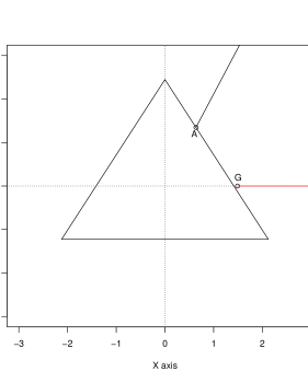
Figure 1: Ternary diagram showing the zero projection. We want to evaluate the line integral of the multivariate normal distribution from A to $\infty$ along the black line. For this reason we rotate the point onto the X-Axis and find the integral from G to $\infty$.

3.2 Example 1. Simulated data

Figure 2 shows a simulated example of the zero-censored model. Data of size $500$ were generated from the following multivariate normal

$$N_{2}\left(\begin{array}[]{cc}(0.625,&0.821)\end{array},\left(\begin{array}[]{cc}0.149&-0.200\\ -0.200&1.523\end{array}\right)\right).$$

When an observation fell outside the simplex it was ”pulled” to the boundary, moving along the line connecting the point with the center of the simple, via the technique described in Tsagris and Stewart (2020). There were $197$ such cases in the data. We applied the zero-censored model to the data by maximizing the log-likelihood (8). We estimated $194$ zeros ($194$ compositional vectors having one element with a zero value). We generated $500$ vectors from a multivariate normal and counted the number of vectors that fell outside the simplex. The estimated parameters of this normal distribution, used in this random vector generation, were

$$\hat{\boldsymbol{\mu}}=\left(0.656,0.788\right)\ \ \text{and}\ \ {\bf S}=\left(\begin{array}[]{cc}0.129&-0.132\\ -0.132&1.477\end{array}\right).$$

Figure 2 shows the ternary plot of the data along with the contours of the zero-censored model calculated from the estimated parameters.

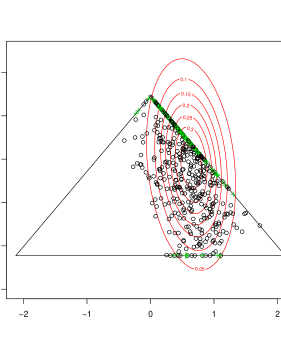
Figure 2: Ternary diagram where the green crosses indicate the points which lie on the boundaries of the simplex. The contour plots of the normal based on the estimated parameters are shown.

A key thing we have to mention about Figure 2 is that the contour lines look vertical but have in fact a negative slope. This is not seen because of the scaling of the ternary plot. The range of values of the x-axis is larger than the range of the simulated values in the first variable and thus the contour lines do not depict the negative slope they should.

3.3 Example 2. Time budget data

We will illustrate the performance of the zero-censored model using real data (Härdle and Hlávka, 2007). There are $28$ individuals and for each person information about the time allocation in $10$ activities is known. The individuals are identified according to gender, country where they live, professional activity, and matrimonial status. We are not interested in their categorization but in the amount of time each person spent on $10$ categories of activities over $100$ days (the total is $100\times 24=2400$ hours fixed for every row) in $1976$. The special feature of these data is that they contain some zero values. Some activities have zero allocation, for instance one woman did not spend even an hour on transportation linked to professional activity and four women did not spend any hour on occupation linked to children. This means that we have five compositions which have one zero in one component only.

The estimated parameters are

$$\hat{\boldsymbol{\mu}}=\left(1.075,-0.030,0.860,0.3830.367,0.222,-2.417,0.568,-0.465\right)\ \ \text{and}$$

$$\hat{\boldsymbol{\Sigma}}=\left[\begin{array}[]{ccccccccc}0.289&0.574&0.109&0.076&0.019&0.035&0.038&0.008&0.030\\ 0.574&1.240&0.200&0.119&0.020&0.063&0.069&-0.020&0.002\\ 0.109&0.200&0.050&0.035&0.013&0.020&0.019&0.015&0.019\\ 0.076&0.119&0.035&0.037&0.013&0.009&0.013&0.015&0.027\\ 0.019&0.020&0.013&0.013&0.008&0.007&0.008&0.010&0.014\\ 0.035&0.063&0.020&0.009&0.007&0.020&0.018&0.010&0.010\\ 0.038&0.069&0.019&0.013&0.008&0.018&0.021&0.005&0.019\\ 0.008&-0.020&0.015&0.015&0.010&0.010&0.005&0.029&0.003\\ 0.030&0.002&0.019&0.027&0.014&0.010&0.019&0.003&0.079\\ \end{array}\right].$$

3.4 Diagnostics for the zero-censored model

We have performed a similar goodness of fit diagnostic to the one Butler and Glasbey (2008) performed. We generated data from the fitted multivariate normal model and estimated the number of zeros in each component. For the first example with the simulated data we had $197$ out of $500$ vectors with one zero element, $171$, $6$ and $20$ zeros in the first, second and third component respectively. The corresponding percentages are $\left(0.342,0.012,0.040\right)$. We estimated the percentages of the zero values in each component to be $\left(0.347,0.008,0.040\right)$ respectively based on $10,000,000$ simulated observations. We repeated the same procedure for the real data in the second example and the results are presented in Table 1.

Table 1: Observed and estimated number of zeros for every component

Components	prof	tran	hous	kids	shop	pers	eat	slee	tele	leis
Observed
number of zeros	0	1	0	4	0	0	0	0	0	0
Estimated
number of zeros	0.593	0.547	2.106	2.151	0.002	0.000	0.000	0.000	0.137	0.000

From Table 1 we see that there is evidence to support the hypothesis that the fit of the model is not to be rejected. We could also use the $\chi^{2}$ test statistic as a discrepancy measure between the estimated and the observed frequencies and a $p$-value could be calculated via simulations or via the $\chi^{2}$ distribution.

4 Conclusions

We developed a parametric zero-censored model for compositional data with zero values. The use of another multivariate model, such as the multivariate skew normal distribution (Azzalini and Valle, 1996) could also be utilized but the difficulty with this distribution is that more parameters need to be estimated, thus making the estimation procedure more difficult. This of course does not exclude the possibility of using this model.

The zero-censored model attacks the problem of zeros from a different perspective than the one Butler and Glasbey (2008) suggested. The data are projected on to the faces of the simplex using a non-orthogonal $1:1$ projection in contrast to the orthogonal Butler and Glasbey (2008) proposed. The advantage over Butler and Glasbey’s approach is that it is not difficult to project the data onto the edges regardless of the dimension. Both models however share the same problem, that of estimating the parameters of the normal distribution which becomes harder as the dimension increases. Both the zero-censored model (9) and the Butler and Glasbey’s model avoid the use of the log-ratio methodology or imputation of the zero values. A limitation of the zero-censored model is that it only allows for one zero per compositional vector. For instance if we have $D=3$ or $D=10$ components, only one zero should be present in each vector.

A further question when modelling compositional data by using either the proposed zero-censored model or the Butler and Glasbey (2008) model, is how to include covariates. Scealy and Welsh (2011b) defined an alternative model based on the Kent distribution which offers the possibility for regression and handling zeros conveniently, at the cost of computational complexity.

References

- Aitchison (1982) Aitchison, J. (1982). The statistical analysis of compositional data. Journal of the Royal Statistical Society: Series B, 44(2):139–177.
- Aitchison (2003) Aitchison, J. (2003). The statistical analysis of compositional data. Reprinted by The Blackburn Press.
- Azzalini and Valle (1996) Azzalini, A. and Valle, A. (1996). The multivariate skew-normal distribution. Biometrika, 83(4):715.