Riesz-Quincunx-Unet Variational Auto-Encoder for Satellite Image Denoising

Abstract

Multiresolution deep learning approaches, such as the U-Net architecture, have achieved high performance in classifying and segmenting images. However, these approaches do not provide a latent image representation and cannot be used to decompose, denoise, and reconstruct image data. The U-Net and other convolutional neural network (CNNs) architectures commonly use pooling to enlarge the receptive field, which usually results in irreversible information loss. This study proposes to include a Riesz-Quincunx (RQ) wavelet transform, which combines 1) higher-order Riesz wavelet transform and 2) orthogonal Quincunx wavelets (which have both been used to reduce blur in medical images) inside the U-net architecture, to reduce noise in satellite images and their time-series. In the transformed feature space, we propose a variational approach to understand how random perturbations of the features affect the image to further reduce noise. Combining both approaches, we introduce a hybrid RQUNet-VAE scheme for image and time series decomposition used to reduce noise in satellite imagery. We present qualitative and quantitative experimental results that demonstrate that our proposed RQUNet-VAE was more effective at reducing noise in satellite imagery compared to other state-of-the-art methods. We also apply our scheme to several applications for multi-band satellite images, including: image denoising, image and time-series decomposition by diffusion and image segmentation.

Keywords: Quincunx wavelet, high order Riesz transform, image time series decomposition, variational auto-encoder, deep neural networks, Sentinel-2, Unet

I Introduction

The temporal frequency of medium resolution, optical satellite imagery, such as Landsat 8 and 9 and Sentinel2A& B, has increase significant in the past four years from one observation every 16 days with Landsat 8 to an observation every 2.9 days on average [16, 25]. Such time series of multi-spectral satellite data enables many novel applications such as global agriculture monitoring and land cover change at the appropriate resolution of land management impacts that has not been possible with low resolution (250-500m GSD) time-series such as MODIS [14, 28, 37]. Moreover, the harmonized Landsat Sentinel2 products open up new avenues for real-time monitoring of a wider variety of change phenomenon [5]. There is a wide variety of time series analysis methods for change detection, which focus primarily on the temporal domain while the spatial domain has been largely neglected (for review see [46]). The availability of hyper-temporal medium resolution imagery allows new application in the spatial domain, such as semantic segmentation with UNET [24] to track objects of change through time.

Change detection methods are hampered by significant noise in the time series that remains despite various processing efforts to reduce the noise [46]. This noise is firstly caused by clouds, and cloud shadows that result in data gaps even when they are correctly detected and serious change artifacts are caused when some clouds or their edges remain undetected [26]. Second, atmospheric variability, notably water vapor and aerosols that cause variability in top of atmosphere reflectance, despite best efforts at atmospheric correction [39, 45]. Third, BRDF variation due to variation in sun-sensor geometry and non-Lambertian reflectance properties of the target. Fourth, variations in spectral reflectance due to seasonal vegetation phenology, which become hard to model when clouds result in missing data that makes the time-series irregular and unpredictable. These issues are often addressed by multi-date composites or temporal interpolation to fill in clouds, shadows and other missing data. Despite efforts to reduce the impact of spatio-temporal noise in the satellite time series, it often limits the accuracy of timely land cover change detection over very large areas using either conventional time-series analysis [42], as well as the new generation of machine learning methods [46].

Various cutting-edge techniques have been developed for image decomposition that can be used to remove noise from conventional images or videos, for example, wavelet smoothing techniques [36, 8, 2] and regularization methods [27], but these methods require parameter selection that vary greatly between datasets and cannot optimally represent varying signals over space and time commonly found in earth observation images. On the other hand, a neural network (UNet) can automatically learn optimal local representation of signal and noise [24, 32], but incurs high computational cost and requires prohibitively large sets of domain-specific training data. The approach proposed in this paper combines the strengths of convolutional neural networks and conventional smoothing techniques. For this purpose we introduce a novel non-subsampled high order Riesz-Quincunx wavelet with variational auto-encoder UNet (RQUNet-VAE) as a hybrid combination of deterministic wavelet expansion (two-dimensional Riesz transformation [36], Quincunx wavelet) and a variational version of a convolutional neural network [22]. The proposed RQUNet-VAE approach uses framelet decomposition [43] to map an image into a sparse feature space and leverages UNet [24] to enable learning of the frames of the feature space. The rationale is that such a hybrid method should provide better feature representation and artifact reduction compared to conventional approaches. Therefore, while previous studies used UNet-VAE for image segmentation [15], we use it to mimic the properties of latent factor model in our RQUNet-VAE decomposition.

To implement this concept, we first introduce a non-subsampled version of high-order Riesz wavelet expansion [36, 34, 35] with Quincunx sampling [8]. Quincunx sampling is used to reduce redundancy of an expansion while high order Riesz transform is used to increase the directional property of wavelet expansion. The hybrid model reduces computational cost with deterministic bases as predefined parameters instead of letting all bases be learnable parameters.

Next, this Riesz-Quincunx wavelet is integrated into the skip-connections of the deep neural network UNet-VAE [13, 15, 7] for learning new bases from the training dataset. Our rationale of using wavelet expansion is that signals extracted from the UNet-VAE encoder, at the skip-connection level, contains both the main signal and details (as well as noise) of an input image which are separated into scaling and wavelet coefficients. Truncation of these coefficients eliminates small wavelet coefficients which contain noise and detailed texture. By decoding the remaining coefficients back into image space, we obtain a denoised version of the original image.

The theoretical framework of RQUNet-VAE is based on Hankel matrix algebra [20], framelet decomposition [43, 44] and proximal operators [21]. Framelet decomposition uses isotropic family-matrix convolution to combine all channels of a multi-band image in a convolutional operation with learnable frames. Furthermore, there is a connection between framelet decomposition and sampling with a finite rate of innovation [40] via Hankel matrix theory and annihilating filter. We prove that RQUNet-VAE also relates to latent factor model whose loss function is defined by Kullback-Leibler divergence [38].

Finally we demonstrate how to apply our proposed RQUNet-VAE to satellite image time series, that is, sequences of images of the same area. Reducing noise satellite image time series is challenging due to the severe background noise resulting from spectral variability caused by changing environmental conditions due to atmospheric and seasonal variability, remaining small clouds, as well as variable sun-sensor geometry [25, 45]. The level of noise is very different from that of conventional videos which contains slow motion changes between subsequent images that can be removed with time delay embedding, for example. In contrast, the satellite time series are constituted by discrete frames that are independently capture several days apart, causing large variability in reflectance properties of the background and objects.

To test the effectiveness of our proposed concept, the RQUNet-VAE was applied to image decomposition, image denoising and segmentation of satellite images and their time-series. Our experimental results show that our hybrid method provides better feature representation and artifact reduction than traditional approaches. The objectives of this paper are:

1. introduce RQUNet-VAE as a generalized wavelet expansion approach;

2. extend RQUnet-VAE to a diffusion process [23] and enable spectral decomposition [9];

3. apply it to image denoising and segmentation in noisy environment for multi-band satellite images and their time-series.

Organization of the paper is: Section II provides the RQUNet-VAE expansion, including mathematical properties and image or time-series decomposition; Section III gives numerical examples and comparisons of image denoising and segmentation in noisy environments for multi-band satellites images. Section IV gives the conclusions, Mathematical background, proofs, and additional experiments are are provided in our supplemental material (SM).

II Riesz-Quincunx-UNet variational auto-encoder (RQUNet-VAE )

II-A Notations and Definitions:

The following list provides an overview of notations used throughout this work.

• continuous coordinate in the spatial domain: $x=(x_{1}\,,x_{2})\in\mathbb{R}^{2}$,

• discrete coordinate in the spatial domain: $k=(k_{1}\,,k_{2})\,,m=(m_{1}\,,m_{2})\in\mathbb{Z}^{2}$,

• Fourier coordinate: $\omega=(\omega_{1}\,,\omega_{2})\in[-\pi\,,\pi]^{2}$,

• Complex number: $j=\sqrt{-1}$,

• Image domain: $\Omega=\{1\,,\ldots\,,n_{1}\}\times\{1\,,\ldots\,,n_{2}\}$, $\mathinner{\!\left\lvert\Omega\right\rvert}=n_{1}\times n_{2}$,

• Images and stacks of images:

  • a gray-scale image $\underline{f}=\begin{pmatrix}f_{1}&\ldots&f_{n_{2}}\end{pmatrix}\in\mathbb{R}^{\mathinner{\!\left\lvert\Omega\right\rvert}}\,,f_{i}\in\mathbb{R}^{n_{1}}$,

  • a multi-channel image $\underline{\underline{f}}=\left\{\underline{f_{1}}\,,\ldots\,,\underline{f_{P}}\right\}\in\mathbb{R}^{\mathinner{\!\left\lvert\Omega\right\rvert}\times P}\,,\underline{f_{i}}\in\mathbb{R}^{\mathinner{\!\left\lvert\Omega\right\rvert}}$,

  • a set of observed images $\textfrak{F}\mathrel{\mathop{\mathchar 58\relax}}=\underline{\underline{\underline{f}}}=\left\{\underline{\underline{f_{i}}}\right\}_{i=1}^{T}\in\mathbb{R}^{\mathinner{\!\left\lvert\Omega\right\rvert}\times P\times T}$,

• Distribution and Lebesgue density: $\underline{f}\stackrel{{\scriptstyle\text{i.i.d.}}}{{\sim}}\mathbb{P}\left(\underline{f}\right)\mathrel{\mathop{\mathchar 58\relax}}=\mathbb{P}\left(\text{d}\underline{f}\right)=\mathtt{p}\left(\underline{f}\right)\text{d}\underline{f}$,

• Continuous Fourier transform of a continuous function $a\in L_{2}(\mathbb{R}^{2})$ is:

  $$a(x) \stackrel{{\scriptstyle{\mathcal{F}}}}{{\longleftrightarrow}}\widehat{a}(\omega)=\int_{\mathbb{R}^{2}}a(x)e^{-j\langle x\,,\omega\rangle_{\ell_{2}}}\text{d}x\,,$$

  and its discrete version is computed via Poisson summation formulae:

  $$a[k] \mathrel{\mathop{\mathchar 58\relax}}=a(x)\mid_{x=k\in\mathbb{Z}^{2}}$$

  $$\stackrel{{\scriptstyle{\mathcal{F}}}}{{\longleftrightarrow}}\widehat{A}\left(e^{j\omega}\right) =\sum_{k\in\mathbb{Z}^{2}}a[k]e^{-j\langle k\,,\omega\rangle_{\ell_{2}}}=\sum_{k\in\mathbb{Z}^{2}}\widehat{a}(2\pi k+\omega)\,.$$

Additional definitions can be found in the supplemental material.

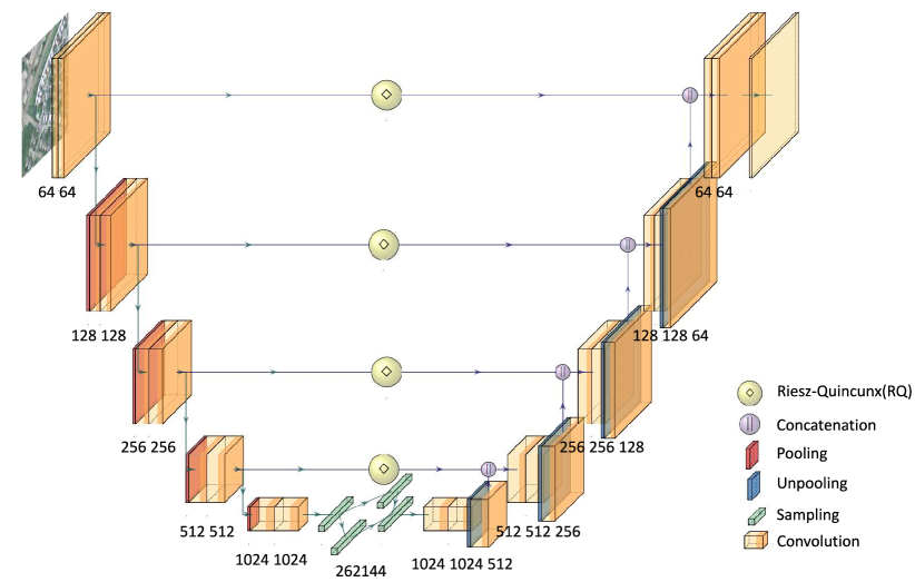
Figure 1: RQUNet-VAE architecture.

II-B RQUNet-VAE Architecture Overview

The network architecture of our proposed RQUNet-VAE is illustrated in Figure 1. The network utilizes a UNet [24] as our primary backbone architecture with the modified skip-connection signals, between the encoder and decoder paths, and bottom layer. The network introduces the Variational Autoencoder (VAE) in the bottom layer to learn the signal distribution in the latent space during training on large datasets. The VAE layer combined with the UNet backbone allows the model to learn and retain much of the input information, similar to generative models, to perform image reconstruction. The reconstructed image then can go through a convolution layer, or a classifier, to produce the final classification or segmentation output. The primary objective of our proposed network is to remove certain levels of noise in the input images in order to produce improved, quality reconstructed images using the Riesz-Quincunx (RQ) scheme in the skip-connections, before performing image classification. Since the RQ scheme is computational heavy, we only applied the RQ computation on a pre-trained network to produce predictions on input images.

II-C $N$-th order Riesz Quincunx non-subsampled wavelet

Before proposing our RQUNet-VAE expansion, we firstly introduce framelet decomposition [43] in the following proposition.

Proposition II.1.

Given an image $\underline{f}\in\mathbb{R}^{n_{1}\times n_{2}}$, all wavelet filter banks $\underline{\Phi}\,,\underline{\tilde{\Phi}}\in\mathbb{R}^{n_{2}d_{1}\times d_{2}}$ (see definitions of wavelet filter banks in Section 4 of the supplemental material) and local basis $\underline{\Xi}\,,\underline{\tilde{\Xi}}\in\mathbb{R}^{n_{1}\times d}$ (see Equation 5 in the supplemental material for details) satisfy the unity conditions

$$\underline{\tilde{\Xi}}\,\underline{\Xi}^{\text{T}} =\sum_{i=1}^{d}\tilde{\xi}_{i}\xi_{i}^{\text{T}}=\text{Id}_{n_{1}\times n_{1}}\,,~{}\underline{\Phi}\,\underline{\tilde{\Phi}}^{\text{T}}=\sum_{i=1}^{d_{2}}\tilde{\phi}_{i}\phi_{i}^{\text{T}}=\text{Id}_{n_{2}d_{1}\times n_{2}d_{1}}$$ (1)

then, a framelet decomposition is:

$$\underline{f} =\mathscr{H}^{\dagger}_{d_{1}\mid n_{2}}\left(\underline{\tilde{\Xi}}\underline{c_{f}}\tilde{\Phi}^{\text{T}}\right)$$

$$=\frac{1}{d_{1}}\sum_{s=1}^{d_{2}}\sum_{l=1}^{d}\sum_{i=1}^{n_{2}}\begin{pmatrix}\left\langle f_{k}\,,\mathfrak{C}_{\phi_{s}^{i}}\left(\xi_{l}\right)\right\rangle_{\ell_{2}}\mathfrak{C}_{\tilde{\phi}^{1}_{s}}\left(\tilde{\xi}_{l}\right)&\\ \cdot\ldots\cdot\\ \left\langle f_{k}\,,\mathfrak{C}_{\phi_{s}^{i}}\left(\xi_{l}\right)\right\rangle_{\ell_{2}}\mathfrak{C}_{\tilde{\phi}^{n_{2}}_{s}}\left(\tilde{\xi}_{l}\right)\end{pmatrix}$$

$$=\frac{1}{d_{1}}\sum_{s=1}^{d_{2}}\begin{pmatrix}\mathfrak{C}_{\tilde{\phi}^{1}_{s}}\left(\underline{\tilde{\Xi}}c_{f,s}\right)&\ldots&\mathfrak{C}_{\tilde{\phi}^{n_{2}}_{s}}\left(\underline{\tilde{\Xi}}c_{f,s}\right)\end{pmatrix}$$ (2)

where $\mathscr{H}^{\dagger}_{d_{1}\mid n_{2}}$ is the extended Hankel matrix of image f as described in the SM. Framelet coefficients are:

$$\underline{c_{f}} \mathrel{\mathop{\mathchar 58\relax}}=\begin{pmatrix}c_{f,1}&\ldots&c_{f,d_{2}}\end{pmatrix}=\underline{\Xi}^{\text{T}}\mathscr{H}_{d_{1}\mid n_{2}}\left(\underline{f}\right)\underline{\Phi}\,.$$ (3)

Proof.

For self-containment, we provide a proof of Proposition II.1 in Section 5.1. in the SM. ∎

Inspired by Proposition II.1, we introduce the proposed RQUNet-VAE expansion in the following.

Riesz-Quincunx wavelet expansion:

To have wavelet expansion, firstly we provide a definition of frame by isotropic polyharmonic Bspline and $N$-th order Riesz transform, see [36]. In particular, an isotropic polyharmonic B-splines basis is defined in the Fourier domain as: $x\in\mathbb{R}^{2}$,

$$\beta_{\gamma}(x)\stackrel{{\scriptstyle{\mathcal{F}}}}{{\longleftrightarrow}}\widehat{\beta}_{\gamma}(\omega)=\frac{\widehat{V}^{iso}(e^{j\omega})^{\frac{\gamma}{2}}}{\mathinner{\!\left\lVert\omega\right\rVert}^{\gamma}_{\ell_{2}}}$$ (4)

with a 2D localization operator:

$$\widehat{V}^{\text{iso}}(e^{j\omega})=\frac{10}{3}$$

$$-\frac{1}{3}\left[4\cos\omega_{1}+4\cos\omega_{2}+\cos(\omega_{1}+\omega_{2})+\cos(\omega_{1}-\omega_{2})\right]\,.$$

Its dual function is defined via an auto-correlation function: $k\in\mathbb{Z}^{2}$,

$$\tilde{\beta}_{\gamma}(x) \stackrel{{\scriptstyle{\mathcal{F}}}}{{\longleftrightarrow}}\widehat{\tilde{\beta}}_{\gamma}(\omega)=\frac{\widehat{\beta}_{\gamma}(\omega)}{\widehat{A}(e^{j\omega})}\,,~{}$$

$$a(k) \stackrel{{\scriptstyle{\mathcal{F}}}}{{\longleftrightarrow}}\widehat{A}(e^{j\omega})=\sum_{m\in\mathbb{Z}^{2}}\widehat{\beta}_{2\gamma}(2\pi m+\omega)\,.$$ (5)

An impulse response of the $L$-th order Riesz transform is:

$$\mathscr{R}^{l}\{\delta\}(x)~{}\stackrel{{\scriptstyle{\mathcal{F}}}}{{\longleftrightarrow}}~{}\widehat{\mathscr{R}^{l}}(\omega)=(-j)^{L}\sqrt{\frac{L!}{n!(L-l)!}}\frac{\omega_{1}^{l}\omega_{2}^{L-l}}{\left(\omega_{1}^{2}+\omega_{2}^{2}\right)^{\frac{L}{2}}}\,,$$

for $l=0\,,\ldots\,,L$ and where $\delta(\cdot)$ is the Dirac delta function. Secondly, wavelet expansion is defined as follows: Given a 2D dyadic sampling matrix $\underline{\text{D}}=\begin{pmatrix}1&1\\ 1&-1\end{pmatrix}$, we have $\widehat{\rho}_{0}=[0\,,0]^{\text{T}}\,,\widehat{\rho}_{1}=[1\,,0]^{\text{T}}$ and

$$\underline{\text{D}}^{i}=\begin{cases}2^{\frac{i}{2}}\text{Id}_{2}\,,&i\text{ is even}\\ 2^{\frac{i-1}{2}}\underline{\text{D}}\,,&i\text{ is odd}\end{cases}\,,~{}\mathinner{\!\left\lvert\text{det }\underline{\text{D}}^{i}\right\rvert}=2^{i}\,.$$

Non-subsampled scaling and wavelet spaces $\mathcal{V}_{i}^{\text{ns}}=\text{span}_{m\in\mathbb{Z}^{2}}\left\{\varphi_{i}\left(\cdot-m\right)\right\}$ and $\mathcal{W}_{il}^{\text{ns}}=\text{span}_{m\in\mathbb{Z}^{2}}\left\{\psi_{il}\left(\cdot-m\right)\right\}$ (for $i=0\,,\ldots\,,I\,;l=0\,,\ldots\,,L$) satisfy a multiscale decomposition $\mathcal{V}_{i-1}^{\text{ns}}=\mathcal{V}_{i}^{\text{ns}}\oplus\sum_{l=0}^{L}\mathcal{W}_{il}^{\text{ns}}\,,i=1\,,\ldots\,,I$ where primal/dual scaling and wavelet functions are:

$$\varphi_{i}(x) =2^{-\frac{i}{2}}\beta_{\gamma}\left(\underline{\text{D}}^{-i}x\right)\,,~{}\tilde{\varphi}_{i}(x)=2^{-\frac{i}{2}}\tilde{\beta}_{\gamma}\left(\underline{\text{D}}^{-i}x\right)\,,$$

$$\psi_{il}(x) =2^{-\frac{i}{2}}\mathscr{R}^{l}\{\psi\}\left(\underline{\text{D}}^{-i}x\right)\,,~{}\tilde{\psi}_{il}(x)=2^{-\frac{i}{2}}\mathscr{R}^{l}\{\tilde{\psi}\}\left(\underline{\text{D}}^{-i}x\right)\,.$$

Their Fourier transforms are

$$\widehat{\varphi}_{i}(\omega) =2^{\frac{i}{2}}\widehat{\beta_{\gamma}}\left(\underline{\text{D}}^{i\text{T}}\omega\right)\,,~{}\widehat{\tilde{\varphi}}_{i}(\omega)=2^{\frac{i}{2}}\widehat{\tilde{\beta}_{\gamma}}\left(\underline{\text{D}}^{i\text{T}}\omega\right)\,,$$

$$\widehat{\psi_{il}}(\omega) =2^{\frac{i}{2}}\widehat{\mathscr{R}^{l}}\left(\underline{\text{D}}^{i\text{T}}\omega\right)\widehat{\psi}\left(\underline{\text{D}}^{i\text{T}}\omega\right)\,,~{}$$

$$\widehat{\tilde{\psi}_{il}}(\omega) =2^{\frac{i}{2}}\widehat{\mathscr{R}^{l}}\left(\underline{\text{D}}^{i\text{T}}\omega\right)\widehat{\tilde{\psi}}\left(\underline{\text{D}}^{i\text{T}}\omega\right)\,.$$

Due to a discrete Fourier transform of continuous functions, by Poisson summation we have the following proposition:

Proposition II.2.

The scaling and wavelet functions satisfy the unity condition in the Fourier domain:

$$\widehat{\tilde{\varphi}}^{*}_{I}(\omega)\widehat{\varphi}_{I}(\omega)+\sum_{i=0}^{I}\sum_{l=0}^{L}\widehat{\tilde{\psi}}^{*}_{il}(\omega)\widehat{\psi}_{il}(\omega)+\widehat{e}(\omega)=1$$ (6)

up to a discretization error:

$$\widehat{e}(\omega)=\widehat{\tilde{\varphi}}^{*}_{I}(\omega)\sum_{k\in\mathbb{Z}^{2}\backslash\{0\}}\widehat{\varphi}_{I}\left(2\pi k+\omega\right)$$

$$+\sum_{m\in\mathbb{Z}^{2}\backslash\{0\}}\widehat{\tilde{\varphi}}^{*}_{I}\left(2\pi m+\omega\right)\left(\widehat{\varphi}_{I}(\omega)+\sum_{k\in\mathbb{Z}^{2}\backslash\{0\}}\widehat{\varphi}_{I}\left(2\pi k+\omega\right)\right)$$

$$+\sum_{i=0}^{I}\sum_{l=0}^{L}\Bigg{[}\widehat{\tilde{\psi}}^{*}_{il}(\omega)\sum_{k\in\mathbb{Z}^{2}\backslash\{0\}}\widehat{\psi}_{il}\left(2\pi k+\omega\right)$$

$$+\sum_{m\in\mathbb{Z}^{2}\backslash\{0\}}\widehat{\tilde{\psi}}^{*}_{il}\left(2\pi m+\omega\right)\left(\widehat{\psi}_{il}(\omega)+\sum_{k\in\mathbb{Z}^{2}\backslash\{0\}}\widehat{\psi}_{il}\left(2\pi k+\omega\right)\right)\Bigg{]}\,.$$ (7)

Proof.

We provide a proof of Proposition II.2 in Section 5.2 in SM. ∎

To compensate the error in Equation II.2 in the unity condition (Equation 6), wavelet function at scale $i=0$ is defined as:

$$\widehat{\psi}_{0}(\omega)=\frac{1}{\widehat{\tilde{\psi}}^{*}_{0}(\omega)}\left(1-\widehat{\tilde{\varphi}}^{*}_{I}(\omega)\widehat{\varphi}_{I}(\omega)-\sum_{i=1}^{I}\widehat{\tilde{\psi}}^{*}_{i}(\omega)\widehat{\psi}_{i}(\omega)\right)\,;$$

then, we have a wavelet expansion for an image $f\in\ell_{2}(\mathbb{Z}^{2})$:

$$f[k] =\sum_{m\in\mathbb{Z}^{2}}\left\langle f\,,\tilde{\varphi}_{I}(\cdot-m)\right\rangle_{\ell_{2}}\varphi_{I}(k-m)$$

$$+\sum_{i=0}^{I}\sum_{l=0}^{L}\sum_{m\in\mathbb{Z}^{2}}\left\langle f\,,\tilde{\psi}_{il}(\cdot-m)\right\rangle_{\ell_{2}}\psi_{il}(k-m)\,.$$ (8)

Following [34], primal and dual wavelet functions are defined as:

$$\widehat{\psi}(\omega) =2^{-\frac{1}{2}}\widehat{G}(e^{j\underline{\text{D}}^{-\text{T}}\omega})\widehat{\beta}_{\gamma}(\underline{\text{D}}^{-\text{T}}\omega)\,,$$

$$\widehat{\tilde{\psi}}(\omega) =2^{-\frac{1}{2}}\widehat{\tilde{G}}\left(e^{j\underline{\text{D}}^{-\text{T}}\omega}\right)\widehat{\tilde{\beta}}_{\gamma}(\underline{\text{D}}^{-\text{T}}\omega)\,,$$ (9)

where the refinement and highpass filters are

$$h[k] \stackrel{{\scriptstyle{\mathcal{F}}}}{{\longleftrightarrow}}\widehat{H}(e^{j\omega})=2^{\frac{1}{2}}\frac{\widehat{\beta}_{\gamma}(\underline{\text{D}}^{\text{T}}\omega)}{\widehat{\beta}_{\gamma}(\omega)}\,,$$

$$\tilde{h}[k] \stackrel{{\scriptstyle{\mathcal{F}}}}{{\longleftrightarrow}}\widehat{\tilde{H}}(e^{j\omega})=\frac{\widehat{A}(e^{j\omega})}{\widehat{A}(e^{j\underline{\text{D}}^{\text{T}}\omega})}\widehat{L}(e^{j\omega})\,,$$

$$g[k] \stackrel{{\scriptstyle{\mathcal{F}}}}{{\longleftrightarrow}}\widehat{G}(e^{j\omega})=-e^{-j\omega_{1}}\widehat{H}(e^{-j(\omega+\pi)})\widehat{A}(e^{j(\omega+\pi)})\,,$$

$$\tilde{g}[k] \stackrel{{\scriptstyle{\mathcal{F}}}}{{\longleftrightarrow}}\widehat{\tilde{G}}(e^{j\omega})=-e^{-j\omega_{1}}\frac{\widehat{H}(e^{-j(\omega+\pi)})}{\widehat{A}(e^{j\underline{\text{D}}^{\text{T}}\omega})}\,,$$

and a scaled auto-correlation function is:

$$\widehat{A}(e^{j\text{D}^{\text{T}}\omega}) =\frac{1}{2}\mathinner{\!\left\lvert\widehat{H}(e^{j\omega})\right\rvert}^{2}\widehat{A}(e^{j\omega})+\frac{1}{2}\mathinner{\!\left\lvert\widehat{H}(e^{j(\omega+\pi)})\right\rvert}^{2}\widehat{A}(e^{j(\omega+\pi)})\,.$$ (10)

Non-subsampled Riesz-Quincunx wavelet smoothing and Hankel matrix

Denote $\underline{\mathfrak{C}}_{\underline{\phi}}\mathrel{\mathop{\mathchar 58\relax}}=\underline{\mathfrak{C}}^{*}_{\underline{\varphi_{I}}}\underline{\mathfrak{C}}_{\underline{\tilde{\varphi}_{I}}}$ where a matrix kernel $\underline{\phi}\in\mathbb{R}^{n_{1}\times n_{2}}$ and its matrix form $\underline{\Phi}\mathrel{\mathop{\mathchar 58\relax}}=\underline{\tilde{\Phi}_{I}}\,\underline{\check{\Phi}_{I}^{\text{T}}}$ are defined in Equation 3 in the SM where $\underline{\tilde{\Phi}_{I}}$ and $\underline{\Phi_{I}}$ are matrix forms of $\underline{\tilde{\varphi}_{I}}$ and $\underline{\varphi_{I}}$, respectively. Similarly, we denote wavelet kernel tensors $\underline{\underline{\psi}}=\left\{\psi_{p}\right\}_{p=1}^{P}\mathrel{\mathop{\mathchar 58\relax}}=\left\{\psi_{il}\right\}_{i=0,\ldots,I}^{l=0,\ldots,L}$ and $\underline{\underline{\tilde{\psi}}}=\left\{\tilde{\psi}_{p}\right\}_{p=1}^{P}\mathrel{\mathop{\mathchar 58\relax}}=\left\{\tilde{\psi}_{il}\right\}_{i=0,\ldots,I}^{l=0,\ldots,L}$ with $\underline{\psi_{p}}\,,\underline{\tilde{\psi}_{p}}\in\mathbb{R}^{\mathinner{\!\left\lvert\Omega\right\rvert}}\,(p=1\,,\ldots\,,P)$ and their matrix form are $\underline{\check{\Psi}}=\begin{pmatrix}\underline{\check{\Psi}_{1}}&\ldots&\underline{\check{\Psi}_{P}}\end{pmatrix}$ and $\underline{\tilde{\Psi}}=\begin{pmatrix}\underline{\tilde{\Psi}_{1}}&\ldots&\underline{\tilde{\Psi}_{P}}\end{pmatrix}$ where block element matrices $\underline{\Psi_{p}}\,,\underline{\tilde{\Psi}_{p}}\in\mathbb{R}^{n_{2}n_{1}\times n_{2}}$ are also are defined in Equation 3 in the supplemental material. For an image $\underline{f}\in\mathbb{R}^{n_{1}\times n_{2}}$, from proposition II.1 we have the following proposition:

Proposition II.3.

A non-subsampled Riesz Quincunx wavelet has a form of framelet decomposition (II.1):

$$\underline{f} =\underline{\mathfrak{C}}_{\underline{\phi}}\left(\underline{f}\right)+\underline{\underline{\mathfrak{C}}}^{*}_{\underline{\underline{\psi}}}\circ\text{prox}_{\mu\mathscr{P}}\circ\underline{\underline{\mathfrak{C}}}_{\underline{\underline{\tilde{\psi}}}}\left(\underline{f}\right)$$

$$=n_{1}\mathscr{H}^{\dagger}_{n_{1}\mid n_{2}}\left(\mathscr{H}_{n_{1}\mid n_{2}}\left(\underline{f}\right)\left(\underline{\Phi}+\underline{\tilde{\Psi}}\,\underline{\check{\Psi}^{\text{T}}}\right)\right)\,.$$ (11)

Scaling and wavelet filter bank matrices satisfy the unity condition:

$$\underline{\Phi}+\underline{\tilde{\Psi}}\,\underline{\check{\Psi}^{\text{T}}}=\frac{1}{n_{1}}\text{Id}_{n_{1}n_{2}\times n_{1}n_{2}}\,.$$ (12)

Proof.

We provide a proof of Proposition II.3 in Section 5.3 in SM. ∎

A smoothing version of a framelet decomposition (Equation II.3) is defined with proximity operators $\text{prox}_{\mu\mathscr{P}}\,(\text{for }\mu>0)$ (as defined in Equation 13 in the supplemental material):

$$\underline{\tilde{f}} =n_{1}\mathscr{H}^{\dagger}_{n_{1}\mid n_{2}}\left(\mathscr{H}_{n_{1}\mid n_{2}}\left(\underline{f}\right)\underline{\Phi}+\text{prox}_{\mu\mathscr{P}}\left\{\mathscr{H}_{n_{1}\mid n_{2}}\left(\underline{f}\right)\underline{\tilde{\Psi}}\right\}\underline{\check{\Psi}^{\text{T}}}\right)\,.$$

Its iterative scheme, called generalized intersection algorithm with fixpoints is described in [23].

II-D RQUNet-VAE expansion

Given a multi-channel image $\underline{\underline{f}}=\left\{\underline{f_{1}}\,,\ldots\,,\underline{f_{P}}\right\}\in\mathbb{R}^{\mathinner{\!\left\lvert\Omega\right\rvert}\times P}$, we introduce our RQUNet-VAE expansion via mappings for skip-connecting signal, latent variables, and a reconstructed signal. Then, we propose RQUNet-VAE expansion and its functional space for regularization.

Mappings:

We introduce filter banks in an encoder $\underline{\underline{\underline{\theta^{1(i)}}}}\in\mathbb{R}^{d_{1}\times d_{2}\times P\times 2^{i}L}$ and $\underline{\underline{\underline{\theta^{2(i)}}}}\in\mathbb{R}^{d_{1}\times n_{2}\times P\times 2^{i}L}$ whose matrix forms are $\underline{\underline{\Theta^{1(i)}}}\in\mathbb{R}^{d_{1}d_{2}P\times d_{2}\times 2^{i}L}\,,\underline{\underline{\Theta^{1(i)}}}\in\mathbb{R}^{d_{1}n_{2}P\times n_{2}\times 2^{i}L}$ (as defined in Equation 6 in the supplemental material). Similar for filter banks $\left\{\left(\underline{\underline{\underline{\tilde{\theta}^{1(i)}}}}\,,\underline{\underline{\underline{\tilde{\theta}^{2(i)}}}}\right)\right\}_{i-0}^{I-1}$ in a decoder. For batch-normalization and dropout layers, we refer the readers to [11, 29].

a.1. Skip-connecting signal (encoder): Given a local basis $\underline{\Xi^{(i)}}$ and an analysis operator at scale $i=1\,,\ldots\,,I$:

$$\mathscr{T}^{(i)} \mathrel{\mathop{\mathchar 58\relax}}=\mathscr{R}_{p}\circ\mathscr{B}\circ\text{prox}_{\text{ReLU}}\circ\underline{\underline{\underline{\mathfrak{C}}}}^{\text{iso}}_{\underline{\underline{\underline{\theta^{2(i)}}}}}\circ\text{prox}_{\text{ReLU}}\circ\underline{\underline{\underline{\mathfrak{C}}}}^{\text{iso}}_{\underline{\underline{\underline{\theta^{1(i)}}}}}$$

$$\,\mathrel{\mathop{\mathchar 58\relax}}\,\mathbb{R}^{n_{1}\times n_{2}\times P}\rightarrow\mathbb{R}^{2^{-i}n_{1}\times 2^{-i}n_{2}\times 2^{i}L}\,,$$ (13)

we define an iterated mapping:

$$\mathscr{C}^{(i)} =\mathscr{T}^{(i)}\circ\underline{\Xi^{(i-1),\text{T}}}\mathscr{T}^{(i-1)}\circ\ldots\circ\underline{\Xi^{(1),\text{T}}}\mathscr{T}^{(1)}$$

$$\,\mathrel{\mathop{\mathchar 58\relax}}\,\mathbb{R}^{n_{1}\times n_{2}\times P}\rightarrow\mathbb{R}^{2^{-(i-1)}n_{1}\times 2^{-(i-1)}n_{2}\times 2^{(i-1)}L}\,.$$

Then, we have the following proposition describing a mapping for the skip-connecting signal:

Proposition II.4.

A mapping for skip-connecting signal in RQUnet-VAE is:

$$\mathscr{C}_{\gamma_{c}}\,\mathrel{\mathop{\mathchar 58\relax}}\,\mathbb{R}^{n_{1}\times n_{2}\times P}\rightarrow\left\{\mathbb{R}^{2^{-(i-1)}n_{1}\times 2^{-(i-1)}n_{2}\times 2^{(i-1)}L}\right\}_{i=1}^{I}\,;$$

$$\underline{\underline{\underline{c}}}=\mathscr{C}_{\gamma_{c}}\left(\underline{\underline{f}}\right)=\left\{\underline{\underline{c^{(i)}}}=\mathscr{C}^{(i)}\left(\underline{\underline{f}}\right)\right\}_{i=0}^{I-1}=\underline{\mathfrak{C}}_{\underline{\phi}}\left(\underline{\underline{\underline{c}}}\right)+\underline{\underline{\mathfrak{C}}}^{*}_{\underline{\underline{\psi}}}\underline{\underline{\mathfrak{C}}}_{\underline{\underline{\tilde{\psi}}}}\left(\underline{\underline{\underline{c}}}\right)$$ (14)

which is equivalent to:

$$\underline{\underline{c^{(i)}}} =\left\{\underline{c^{(i)}_{l}}\right\}_{l=0}^{2^{i-1}L-1}\,,~{}\underline{c^{(i)}_{l}}=\underline{\mathfrak{C}}_{\underline{\phi}}\left(\underline{c^{(i)}_{l}}\right)+\underline{\underline{\mathfrak{C}}}^{*}_{\underline{\underline{\psi}}}\underline{\underline{\mathfrak{C}}}_{\underline{\underline{\tilde{\psi}}}}\left(\underline{c^{(i)}_{l}}\right)$$

for $i=0\,,\ldots\,,I-1$ where unknown filter banks are $\gamma_{c}\mathrel{\mathop{\mathchar 58\relax}}=\left\{\left(\underline{\underline{\underline{\theta^{1(i)}}}}\,,\underline{\underline{\underline{\theta^{2(i)}}}}\right)\right\}_{i=1}^{I}$.

Proof.

We provide a proof of Proposition II.4 in Section 5.4 in SM. ∎

a.2. Variational term (encoder): We firstly define linear mappings as a perceptron network for latent variable:

$$\mathscr{F}^{\mu}(\cdot) =\underline{W^{\mu}}\text{vec}(\cdot)+b^{\mu}\,,$$

$$\mathscr{F}^{\sigma}(\cdot) =\underline{W^{\sigma}}\text{vec}(\cdot)+b^{\sigma}\,\mathrel{\mathop{\mathchar 58\relax}}\,\mathbb{R}^{2^{-i-1}n_{1}\times 2^{-i-1}n_{2}\times 2^{i}L}\rightarrow\mathbb{R}^{d}\,;$$ (15)

where $\underline{W^{\mu}}\,,\underline{W^{\sigma}}\in\mathbb{R}^{d\times 2^{-(I+1)}n_{1}n_{2}L}$ and $b^{\mu}\,,b^{\sigma}\in\mathbb{R}^{d}$ and $d$ is latent dimension and $\text{vec}(\cdot)$ is a vectorize operation. Denote Hadamard product $\odot$ and model’s parameters as:

$$\gamma_{c}\cup\gamma_{s}\cup\gamma_{m}\mathrel{\mathop{\mathchar 58\relax}}=\left\{\underline{W^{\mu}}\,,b^{\mu}\,,\underline{W^{\sigma}}\,,b^{\sigma}\,,\left\{\left(\underline{\underline{\underline{\theta^{1(i)}}}}\,,\underline{\underline{\underline{\theta^{2(i)}}}}\right)\right\}_{i=1}^{I}\right\}\,;$$

then, we have the following proposition for a variational term:

Proposition II.5.

A latent variable in RQUnet-VAE is sampled from a distribution:

$$z =\mathscr{M}_{\gamma_{m}}\left(\underline{\underline{f}}\right)+\mathscr{S}_{\gamma_{s}}^{\frac{1}{2}}\left(\underline{\underline{f}}\right)\odot\epsilon\,,~{}\epsilon\stackrel{{\scriptstyle\text{i.i.d.}}}{{\sim}}\mathcal{N}_{d}\left(\mathbf{0}_{d}\,,\text{Id}_{d}\right)$$ (16)

where maps for the mean and variance for the latent variable are:

$$\mathscr{M}_{\gamma_{m}}\mathrel{\mathop{\mathchar 58\relax}}=\mathscr{F}^{\mu}\circ\mathscr{R}_{p}\circ\underline{\Xi^{(I),\text{T}}}\mathscr{T}^{(I)}\circ\ldots\circ\underline{\Xi^{(1),\text{T}}}\mathscr{T}^{(1)}\,,$$ (17)

$$\mathscr{S}_{\gamma_{s}}^{\frac{1}{2}}\mathrel{\mathop{\mathchar 58\relax}}=\mathscr{F}^{\sigma}\circ\mathscr{R}_{p}\circ\underline{\Xi^{(I),\text{T}}}\mathscr{T}^{(I)}\circ\ldots\circ\underline{\Xi^{(1),\text{T}}}\mathscr{T}^{(1)}\,.$$ (18)

Proof.

We provide a proof of Proposition II.5 in Section 5.5 in SM. ∎

a.3. Decoder: Firstly, we define a mapping in the decoder:

$$\tilde{\mathscr{T}}^{(i)} =\left(\mathcal{Z}_{1}^{-1}\,,\text{prox}_{\text{ReLU}}\circ\underline{\underline{\underline{\mathfrak{C}}}}^{\text{iso}}_{\underline{\underline{\underline{\tilde{\theta}^{1(i+1)}}}}}\circ\text{prox}_{\text{ReLU}}\circ\underline{\underline{\underline{\mathfrak{C}^{\text{iso}}}}}_{\underline{\underline{\underline{\tilde{\theta}^{2(i+1)}}}}}\circ\mathscr{P}_{\underline{\tilde{\Xi}^{(i)}_{\text{aug}}}}\right),$$

$$\tilde{\mathscr{T}}^{(0)} =\text{prox}_{\text{ReLU}}\circ\underline{\underline{\underline{\mathfrak{C}}}}^{\text{iso}}_{\underline{\underline{\underline{\tilde{\theta}^{1(1)}}}}}\circ\text{prox}_{\text{ReLU}}\circ\underline{\underline{\underline{\mathfrak{C}^{\text{iso}}}}}_{\underline{\underline{\underline{\tilde{\theta}^{2(1)}}}}}\circ\mathscr{P}_{\underline{\tilde{\Xi}^{(0)}_{\text{aug}}}}\,,$$

where $\mathcal{Z}_{1}^{-1}$ is scale-delayed 1 step back of the 1st argument and a concatenate layer is defined as an operation $\mathscr{P}_{\underline{\tilde{\Xi}^{(i)}_{\text{aug}}}}\left(\underline{\underline{\widehat{c}^{(i)}_{\text{aug}}}}\right)=\begin{pmatrix}\underline{\underline{c^{(i)}}}&\mathscr{B}\circ\underline{\tilde{\Xi}^{(i)}}\,\underline{\underline{\widehat{s}^{(i+1)}}}\end{pmatrix}$, i.e. input signal at concatenation layer includes bypass signal $c^{(i)}$ and unpooled-batchnormed lowpass signal $\mathscr{B}\circ\underline{\tilde{\Xi}^{(i)}}\,\underline{\underline{\widehat{s}^{(i+1)}}}$.

Next, we define an iterated mapping for a skip-connecting signal $\underline{\underline{\underline{c}}}$ and a lowpass signal $\underline{\underline{s^{(I)}}}$ at scale $I$ as:

$$\tilde{\mathscr{T}}_{I}\left(\underline{\underline{\underline{c}}}\,,\underline{\underline{s^{(I)}}}\right)=\tilde{\mathscr{T}}^{(0)}\circ\tilde{\mathscr{T}}^{(1)}\circ\ldots\circ\tilde{\mathscr{T}}^{(I-1)}\begin{pmatrix}\underline{\underline{c^{(I-1)}}}&\underline{\underline{s^{(I)}}}\end{pmatrix}\,.$$

Note that $\underline{\underline{s^{(I)}}}$ is reconstructed from a latent variable $z$. Denote unknown parameters in a decoder as:

$$\alpha\mathrel{\mathop{\mathchar 58\relax}}=\left\{\underline{W^{s}}\,,b^{s}\,,\underline{\underline{\underline{\theta^{0}}}}\,,\left\{\left(\underline{\underline{\underline{\tilde{\theta}^{1(i)}}}}\,,\underline{\underline{\underline{\tilde{\theta}^{2(i)}}}}\right)\right\}_{i=1}^{I}\right\}\,.$$

Then, we have the following proposition:

Proposition II.6.

Given a skip-connecting signal $\underline{\underline{\underline{c}}}$ and a latent variable $y$ from an encoder, a decoder mapping in RQUNet-VAE is defined as

$$\mathscr{D}_{\alpha}\left(\underline{\underline{\underline{c}}}\,,z\right) \mathrel{\mathop{\mathchar 58\relax}}=\text{prox}_{\text{ReLU}}\circ\underline{\underline{\underline{\mathfrak{C}}}}^{\text{iso}}_{\underline{\underline{\underline{\theta^{0}}}}}\circ\tilde{\mathscr{T}}_{I}\left(\underline{\underline{\underline{c}}}\,,\text{uvec}\left(\underline{W^{s}}\,z+b^{s}\right)\right)\,.$$ (19)

Proof.

We provide a proof of Proposition II.6 in Section 5.6 in SM. ∎

RQUNet-VAE expansion

An auto-encoder is recast as a latent factor model (a decoder) whose latent variable is computed from the observed data as an encoder:

$$z =\mathscr{M}_{\gamma_{m}}\left(\underline{\underline{f}}\right)+\mathscr{S}_{\gamma_{s}}^{\frac{1}{2}}\left(\underline{\underline{f}}\right)\odot\epsilon\,,~{}\epsilon\stackrel{{\scriptstyle\text{i.i.d.}}}{{\sim}}\mathcal{N}_{d}(\mathbf{0}_{d}\,,\text{Id}_{d})\,,~{}$$ (20)

$$\underline{\underline{\underline{c}}} =\mathscr{C}_{\gamma_{c}}\left(\underline{\underline{f}}\right)\,,$$ (21)

$$\underline{\underline{\tilde{f}}} =\mathscr{D}_{\alpha}\left(\underline{\underline{\underline{c}}}\,,z\right)+\sigma\underline{\underline{e}}\,,~{}\underline{\underline{e}}\stackrel{{\scriptstyle\text{i.i.d.}}}{{\sim}}\mathcal{N}_{\mathinner{\!\left\lvert\Omega\right\rvert}\times P}(0\,,\text{Id})\,,~{}$$ (22)

$$\underline{\underline{\tilde{f}}} =\underline{\underline{f}}\in\textfrak{F}\,,$$ (23)

with a known standard deviation $\sigma>0$ and the data set $\textfrak{F}=\left\{\underline{\underline{f_{i}}}\right\}_{i=1}^{T}\subset\mathbb{R}^{\mathinner{\!\left\lvert\Omega\right\rvert}\times P}$. Combining Equation 22, Equation 20, Equation 21, and Equation 23, we obtain a variational auto-encoder:

$$\underline{\underline{f}} =\mathscr{D}_{\alpha}\left(\mathscr{C}_{\gamma_{c}}\left(\underline{\underline{f}}\right)\,,\mathscr{M}_{\gamma_{m}}\left(\underline{\underline{f}}\right)+\mathscr{S}_{\gamma_{s}}^{\frac{1}{2}}\left(\underline{\underline{f}}\right)\odot\epsilon\right)+\sigma\underline{\underline{e}}\,,$$ (24)

with standard normal random variables $\epsilon\stackrel{{\scriptstyle\text{i.i.d.}}}{{\sim}}\mathcal{N}_{d}(\mathbf{0}_{d}\,,\text{Id}_{d})$ and $\underline{\underline{e}}=\left[e_{l,c}\right]_{l\in\Omega}^{c=1,\ldots,p}\,,e_{l,c}\stackrel{{\scriptstyle\text{i.i.d.}}}{{\sim}}\mathcal{N}(0\,,1)$.

The auto-encoder system (Equations 22-23) is recast as Bayesian inference:

$$\underline{\underline{\tilde{f}}}\mid z\stackrel{{\scriptstyle\text{i.i.d.}}}{{\sim}} \mathcal{N}_{n_{1}\times n_{2}\times P}\left(\mathscr{D}_{\alpha}\left(\underline{\underline{\underline{c}}}\,,z\right)\,,\sigma^{2}\text{Id}\right)$$

$$=\mathbb{H}_{\alpha}\left(\underline{\underline{\tilde{f}}}\mid z\right)=\mathtt{h}_{\alpha}\left(\underline{\underline{\tilde{f}}}\mid z\right)\text{d}\underline{\underline{\tilde{f}}}\,,~{}$$ (25)

$$z\mid\underline{\underline{f}}\stackrel{{\scriptstyle\text{i.i.d.}}}{{\sim}} \mathbb{K}_{\alpha}\left(z\mid\underline{\underline{f}}\right)=\mathtt{k}_{\alpha}\left(z\mid\underline{\underline{f}}\right)\text{d}y$$

$$\approx\,\mathcal{N}_{d}\left(\mathscr{M}_{\gamma_{m}}\left(\underline{\underline{f}}\right)\,,\text{diag}\left\{\mathscr{S}_{\gamma_{s}}\left(\underline{\underline{f}}\right)\right\}\right)\,.$$ (26)

An explanation for the above hierarchical model is: an observed signal $\underline{\underline{\tilde{f}}}$ is assumed to be sampled from a normal distribution whose latent variable $z$ is sampled from an unknown distribution $\mathbb{K}_{\alpha}$ which is approximated by a normal distribution (Equation II-D) parameterized by $(\gamma_{m},\gamma_{s})$. The key idea for $z\mid\underline{\underline{f}}\sim\mathbb{K}_{\alpha}$ to depend on a parameter $\alpha$ is because of the auto-encoder (Equations 20-23), i.e. $\underline{\underline{\tilde{f}}}=\underline{\underline{f}}$. To see this, Bayes’ rule for a conditional density of random variable $z\mid\underline{\underline{f}}$ is:

$$\mathtt{p}\left(z\mid\underline{\underline{f}}\right) =\frac{\mathtt{p}\left(\underline{\underline{f}}\mid z\right)\mathtt{p}(z)}{\mathtt{p}\left(\underline{\underline{f}}\right)}=\frac{\mathtt{p}\left(\underline{\underline{\tilde{f}}}\mid z\right)\mathtt{p}(z)}{\mathtt{p}\left(\underline{\underline{f}}\right)}$$

$$\stackrel{{\scriptstyle(\ref{eq:Decoder:Bayes})}}{{=}}\frac{\mathtt{h}_{\alpha}\left(\underline{\underline{\tilde{f}}}\mid z\right)\mathtt{p}(z)}{\mathtt{p}\left(\underline{\underline{f}}\right)}\mathrel{\mathop{\mathchar 58\relax}}=\mathtt{k}_{\alpha}\left(z\mid\underline{\underline{f}}\right)\,,$$

which depends on a decoder’s parameter $\alpha$. Since the above density is intractible because of the incomputable integral in a marginal distribution $\mathtt{p}\left(\underline{\underline{f}}\right)=\int_{\mathbb{R}^{d}}\mathtt{h}_{\alpha}\left(\underline{\underline{\tilde{f}}}\mid z\right)\mathtt{p}(z)\text{d}z$, a distribution $\mathbb{K}_{\alpha}$ is approximated by a normal distribution:

$$\mathtt{k}_{\alpha}\left(z\mid\underline{\underline{f}}\right) =\frac{\mathtt{h}_{\alpha}\left(\underline{\underline{f}}\mid z\right)\mathtt{p}(z)}{\mathtt{p}\left(\underline{\underline{f}}\right)}$$

$$\approx\mathcal{N}_{d}\left(z\,;\mathscr{M}_{\gamma_{m}}\left(\underline{\underline{f}}\right)\,,\text{diag}\left\{\mathscr{S}_{\gamma_{s}}\left(\underline{\underline{f}}\right)\right\}\right)\,.$$ (27)

Denote variance vector as

$$\mathscr{S}_{\gamma_{s}}\left(\underline{\underline{f}}\right) =\mathscr{S}_{\gamma_{s}}^{\frac{1}{2}}\left(\underline{\underline{f}}\right)\odot\mathscr{S}_{\gamma_{s}}^{\frac{1}{2}}\left(\underline{\underline{f}}\right)$$

$$=\begin{pmatrix}\mathscr{S}_{\gamma_{s}}\left(\underline{\underline{f}}\right)_{1}&\ldots&\mathscr{S}_{\gamma_{s}}\left(\underline{\underline{f}}\right)_{d}\end{pmatrix}^{\text{T}}\in\mathbb{R}^{d}\,.$$

Choose a standard normal prior distribution $\mathbb{P}(z)=\mathtt{p}(z)\text{d}z=\mathcal{N}_{d}\left(\mathbf{0}_{d}\,,\text{Id}_{d}\right)$, we have the following proposition for finding model’s parameters:

Proposition II.7.

Unknown parameters in RQUnet-VAE are obtained from the following minimization problem:

$$\left(\gamma_{c}^{\dagger}\,,\gamma_{m}^{\dagger}\,,\gamma_{s}^{\dagger}\,,\alpha^{\dagger}\right) =\mathop{\rm argmin}\mathscr{L}\left(\gamma_{c}\,,\gamma_{m},\gamma_{s}\,,\alpha\right)$$ (28)

where:

$$\mathscr{L}(\cdot)\mathrel{\mathop{\mathchar 58\relax}}=\frac{1}{2\sigma^{2}}\sum_{i=1}^{T}\mathbb{E}_{\epsilon\sim\mathcal{N}(0\,,\text{Id})}\bigg{[}$$

$$\mathinner{\!\left\lVert\underline{\underline{f_{i}}}-\mathscr{D}_{\alpha}\left(\mathscr{C}_{\gamma_{c}}\left(\underline{\underline{f_{i}}}\right)\,,\mathscr{M}_{\gamma_{m}}\left(\underline{\underline{f_{i}}}\right)+\mathscr{S}_{\gamma_{s}}^{\frac{1}{2}}\left(\underline{\underline{f_{i}}}\right)\odot\epsilon\right)\right\rVert}^{2}_{\ell_{2}}\bigg{]}$$

$$+\sum_{i=1}^{T}\text{KL}\left[\mathcal{N}_{d}\left(\mathscr{M}_{\gamma_{m}}\left(\underline{\underline{f}}\right)\,,\text{diag}\left\{\mathscr{S}_{\gamma_{s}}\left(\underline{\underline{f}}\right)\right\}\right)\mid\mid\mathcal{N}_{d}\left(\mathbf{0}_{d}\,,\text{Id}_{d}\right)\right]$$

and KL-divergence is defined as:

$$\text{KL}\left[\cdot\mid\mid\cdot\right]$$

$$=\frac{1}{2}\left(\mathinner{\!\left\lVert\mathscr{M}_{\gamma_{m}}\left(\underline{\underline{f}}\right)\right\rVert}^{2}_{\ell_{2}}-d+\sum_{i=1}^{d}\left(\mathscr{S}_{\gamma_{s}}\left(\underline{\underline{f}}\right)_{i}-\log\mathscr{S}_{\gamma_{s}}\left(\underline{\underline{f}}\right)_{i}\right)\right)\,.$$ (29)

Proof.

We provide a proof of Proposition II.7 in Section 5.7 in SM. ∎

It is clear that the only one random variable in the above minimization is $\epsilon$, so the gradient descent method can be applied for model parameters $\left(\gamma_{c}\,,\gamma_{m},\gamma_{s}\,,\alpha\right)$. Since high order Riesz-Quincunx wavelet expansion is an identity operator, for training these model parameters, we remove this layer in the training procedure. But, later we use it in its smoothing version with the trained parameters $\left(\gamma_{c}^{\dagger}\,,\gamma_{m}^{\dagger}\,,\gamma_{s}^{\dagger}\,,\alpha^{\dagger}\right)$ to truncate small wavelet coefficients of signals in skip-connection. A summary of RQUNet-VAE with a training procedure (without Riesz-Quincunx wavelet) is shown in the SM for encoder and decoder, respectively.

Generalized Besov space by RQUNet-VAE and proximal operators

We note that Equation 28 is a non-convex minimization problem with potentially many local minimas. Assume an existence of minima $\left(\alpha^{\dagger}\,,\gamma_{c}^{\dagger}\,,\gamma_{m}^{\dagger}\,,\gamma_{s}^{\dagger}\right)$ such that a condition of perfect reconstruction occurs, i.e. $\underline{\underline{\tilde{f}}}=\underline{\underline{f}}$; then, the auto-encoder (Equations 22-23) plays as a generalized wavelet expansion with learnable parameters:

$$\lim_{\sigma\rightarrow 0}\mathinner{\!\left\lVert\underline{\underline{f}}-\mathscr{D}_{\alpha^{\dagger}}\left(\mathscr{C}_{\gamma_{c}^{\dagger}}\left(\underline{\underline{f}}\right)\,,\mathscr{M}_{\gamma_{m}^{\dagger}}\left(\underline{\underline{f}}\right)+\mathscr{S}_{\gamma_{s}^{\dagger}}^{\frac{1}{2}}\left(\underline{\underline{f}}\right)\odot\epsilon\right)+\sigma\underline{\underline{e}}\right\rVert}^{2}_{\ell_{2}}$$

$$=0\,,$$

having its deterministic version:

$$\underline{\underline{f}}=\mathscr{D}_{\alpha^{\dagger}}\left(\mathscr{C}_{\gamma_{c}^{\dagger}}\left(\underline{\underline{f}}\right)\,,\mathscr{M}_{\gamma_{m}^{\dagger}}\left(\underline{\underline{f}}\right)+\mathscr{S}_{\gamma_{s}^{\dagger}}^{\frac{1}{2}}\left(\underline{\underline{f}}\right)\odot\epsilon\right)\,,$$

where encoder and decoder are forward and backward wavelet transform. Then, it induces a generalized Besov space:

$$\textfrak{B}\mathrel{\mathop{\mathchar 58\relax}}=\left\{\underline{\underline{f}}\in\mathbb{R}^{\mathinner{\!\left\lvert\Omega\right\rvert}\times P}\,\mathrel{\mathop{\mathchar 58\relax}}\,\mathinner{\!\left\lVert\underline{\underline{f}}\right\rVert}_{\textfrak{B}}\mathrel{\mathop{\mathchar 58\relax}}=\mathscr{P}\circ\mathscr{C}_{\gamma_{c}}\left(\underline{\underline{f}}\right)<\infty\right\}\,,$$ (30)

where function $\mathscr{P}(\cdot)$ acts on the skip-connecting signal $\underline{\underline{\underline{c}}}=\mathscr{C}_{\gamma_{c}}\left(\underline{\underline{f}}\right)$ for proximal mapping as described in Equation 13 in the supplemental material.

Then, given an image $\underline{\underline{f}}\in\mathbb{R}^{\mathinner{\!\left\lvert\Omega\right\rvert}\times P}$ with an expansion in a space $\textfrak{B}$ (30), we have a regularization in that space $\textfrak{B}$ with the optimally trained parameters as generalized wavelet smoothing via a proximal operator:

$$\underline{\underline{\underline{\tilde{c}}}} =\mathop{\rm argmin}_{\underline{\underline{\underline{w}}}}\left\{\mathscr{P}\left(\underline{\underline{\underline{w}}}\right)+\frac{1}{2\mu}\mathinner{\!\left\lVert\mathscr{C}_{\gamma_{c}}\left(\underline{\underline{f}}\right)-\underline{\underline{\underline{w}}}\right\rVert}^{2}_{\text{F}}\right\}$$

$$=\text{prox}_{\mu\mathscr{P}}\circ\mathscr{C}_{\gamma_{c}}\left(\underline{\underline{f}}\right)$$

$$=\underline{\mathfrak{C}}_{\underline{\phi}}\circ\mathscr{C}_{\gamma_{c}}\left(\underline{\underline{f}}\right)+\underline{\underline{\mathfrak{C}}}^{*}_{\underline{\underline{\psi}}}\circ\text{prox}_{\mu\mathscr{P}}\circ\underline{\underline{\mathfrak{C}}}_{\underline{\underline{\tilde{\psi}}}}\circ\mathscr{C}_{\gamma_{c}}\left(\underline{\underline{f}}\right)\,,$$ (31)

where its element form is:

$$\underline{\underline{\underline{\tilde{c}}}} =\left\{\underline{\underline{\tilde{c}^{(i)}}}\right\}_{i=0}^{I-1}\,,~{}\underline{\underline{\tilde{c}^{(i)}}}=\left\{\underline{\tilde{c}^{(i)}_{l}}\right\}_{l=0}^{2^{i-1}L-1}\,,$$

$$\underline{\tilde{c}^{(i)}_{l}} =\underline{\mathfrak{C}}_{\underline{\phi}}\left(\underline{c^{(i)}_{l}}\right)+\underline{\underline{\mathfrak{C}}}^{*}_{\underline{\underline{\psi}}}\circ\text{prox}_{\mu\mathscr{P}}\circ\underline{\underline{\mathfrak{C}}}_{\underline{\underline{\tilde{\psi}}}}\left(\underline{c^{(i)}_{l}}\right)$$

for $l=0\,,\ldots\,,2^{i-1}L-1\,,~{}i=0\,,\ldots\,,I-1$. Note that $\text{prox}_{\mu\mathscr{P}}(\cdot)$ in Equation II-D acts on wavelet coefficients only. A reason is scaling coefficients contain main energy of a signal whose values are large. These scaling coefficients should be preserved during a shrinking process while wavelet coefficients mainly contain oscillating signals in different scales, including noise which should be removed.

Then, we have a smoothed image as:

$$\underline{\underline{\tilde{f}}}=\mathscr{D}_{\alpha^{\dagger}}\left(\underline{\underline{\underline{\tilde{c}}}}\,,~{}\mathscr{M}_{\gamma_{m}}\left(\underline{\underline{f}}\right)+\mathscr{S}_{\gamma_{s}}^{\frac{1}{2}}\left(\underline{\underline{f}}\right)\odot\epsilon\right)\in\mathbb{R}^{\mathinner{\!\left\lvert\Omega\right\rvert}\times P}\,.$$

In summary, we have the following proposition:

Proposition II.8.

Given a learned parameter $\left(\alpha^{\dagger}\,,\gamma_{c}^{\dagger}\,,\gamma_{m}^{\dagger}\,,\gamma_{s}^{\dagger}\right)$ obtain by training RQUNet-VAE with a dataset, we have RQUNet-VAE smoothing (with a parameter $\mu>0$) for an image $\underline{\underline{\tilde{f}}}$ as a solution of a regularization in a generalized Besov space $\textfrak{B}$ (30):

$$\underline{\underline{\tilde{f}}}=\mathscr{D}_{\alpha^{\dagger}}\bigg{(} \underline{\mathfrak{C}}_{\underline{\phi}}\circ\mathscr{C}_{\gamma_{c}^{\dagger}}\left(\underline{\underline{f}}\right)+\underline{\underline{\mathfrak{C}}}^{*}_{\underline{\underline{\psi}}}\circ\text{prox}_{\mu\mathscr{P}}\circ\underline{\underline{\mathfrak{C}}}_{\underline{\underline{\tilde{\psi}}}}\circ\mathscr{C}_{\gamma_{c}^{\dagger}}\left(\underline{\underline{f}}\right)$$

$$\,,\mathscr{M}_{\gamma_{m}^{\dagger}}\left(\underline{\underline{f}}\right)+\mathscr{S}_{\gamma_{s}^{\dagger}}^{\frac{1}{2}}\left(\underline{\underline{f}}\right)\odot\epsilon\bigg{)}\,.$$ (32)

Proof.

A proof of Proposition II.8 is directly obtained from the above paragraphs. ∎

II-E RQUNet-VAE iterative shrinkage Lagrangian system

Decomposition for multi-band image

RQUNet-VAE   iterative shrinkage algorithm for multi-band image $\underline{\underline{f}}\in\mathbb{R}^{\mathinner{\!\left\lvert\Omega\right\rvert}\times P}$ is described in Algorithm 1 in the SM. This is equivalent to a nonlinear mapping with unknown model’s parameters $\Gamma$: $\underline{\underline{u}}^{(0)}=\underline{\underline{f}}\,,\underline{\underline{\lambda}}^{(0)}=\mathbf{0}$ for $\tau=1\,,\ldots\,,N$ and

$$\left(\underline{\underline{u}}^{(\tau)}\,,\underline{\underline{\lambda}}^{(\tau+1)}\right) =\mathscr{K}_{\mu}\left(\underline{\underline{f}}\,,\underline{\underline{u}}^{(\tau-1)}\,,\underline{\underline{\lambda}}^{(\tau)}\,;\Gamma\right)\,.$$ (33)

Diffusion process and spectral decomposition for multiband image

For a multiband image $\underline{\underline{f}}\in\mathbb{R}^{\mathinner{\!\left\lvert\Omega\right\rvert}\times P}$, a diffusion process by a Lagrangian system (34) is: $\underline{\underline{u}}^{(0)}=\underline{\underline{f}}\,,\tau=1\,,\ldots\,,N$,

$$\left(\underline{\underline{u}}^{(\tau)}\,,\underline{\underline{\lambda}}^{(\tau+1)}\right) =\mathscr{K}_{\mu}\left(\underline{\underline{u}}^{(\tau-1)}\,,\underline{\underline{u}}^{(\tau-1)}\,,\underline{\underline{\lambda}}^{(\tau)}\,;\Gamma\right)\,.$$ (34)

Given $\left\{\underline{\underline{u}}^{(\tau)}\right\}_{\tau=1}^{N}$ generated by diffusion process (34) in Algorithm 2, we have a discrete TV-like transform as in [9]:

$$\underline{\underline{\phi}}^{(\tau)}\mathrel{\mathop{\mathchar 58\relax}}=\frac{\tau}{\beta}\left(\underline{\underline{u}}^{(\tau+1)}-2\underline{\underline{u}}^{(\tau)}+\underline{\underline{u}}^{(\tau-1)}\right)\,,$$

whose inverse transform is: $\underline{\underline{\tilde{f}}}^{(N)}\mathrel{\mathop{\mathchar 58\relax}}=\left(1+N\right)\underline{\underline{u}}^{(N)}-N\underline{\underline{u}}^{(N+1)}$,

$$\underline{\underline{f}}=\underline{\underline{\tilde{f}}}^{(N)}+\beta\sum_{\tau=1}^{N}\underline{\underline{\phi}}^{(\tau)}\,.$$

Its filtered version

$$\underline{\underline{f_{H_{N}}}}=H^{(N)}\underline{\underline{\tilde{f}}}^{(N)}+\beta\sum_{\tau=1}^{N}H^{(\tau)}\underline{\underline{\phi}}^{(\tau)}$$

is defined, e.g. by the ideal spectral-filter $H^{(\tau)}$:

$$H_{\text{lowpass}}^{(\tau)} =\begin{cases}0\,,&\tau\in\{0\,,\ldots\,,\tau_{1}\}\,,\\ 1\,,&\tau\in\{\tau_{1}\,,\ldots\,,N\}\end{cases}\,,$$

$$H_{\text{highpass}}^{(\tau)} =\begin{cases}1\,,&\tau\in\{0\,,\ldots\,,t_{1}\}\,,\\ 0\,,&\tau\in\{\tau_{1}\,,\ldots\,,N\}\end{cases}\,,~{}$$

$$H_{\text{bandpass}}^{(\tau)} =\begin{cases}0\,,&\tau\in\{0\,,\ldots\,,\tau_{1}\}\,,\\ 1\,,&\tau\in\{\tau_{1}\,,\ldots\,,\tau_{2}\}\,,\\ 0\,,&\tau\in\{\tau_{2}\,,\ldots\,,N\}\end{cases}\,,$$

$$H_{\text{bandstop}}^{(\tau)} =\begin{cases}1\,,&\tau\in\{0\,,\ldots\,,\tau_{1}\}\,,\\ 0\,,&\tau\in\{\tau_{1}\,,\ldots\,,\tau_{2}\}\,,\\ 1\,,&\tau\in\{\tau_{2}\,,\ldots\,,N\}\,,\end{cases}$$

where the time threshold $\tau_{i}$ are selected by the TV-spectrum $S^{(\tau)}\mathrel{\mathop{\mathchar 58\relax}}=\mathinner{\!\left\lVert\underline{\underline{\phi}}^{(\tau)}\right\rVert}_{\ell_{1}}$.

Decomposition for multiband time series

Next, we show how our RQUNet-VAE can be applied to satellite image time series, that is, a sequence of images of the same area.

Given a multi-band video $\underline{\underline{\underline{f}}}=\left\{\underline{\underline{f_{1}}}\,,\ldots\,,\underline{\underline{f_{T}}}\right\}\in\mathbb{R}^{\mathinner{\!\left\lvert\Omega\right\rvert}\times P\times T}$, $\underline{\underline{f_{t}}}=\left\{\underline{f_{t,1}}\,,\ldots\,,\underline{f_{t,P}}\right\}$, $\underline{f_{t,p}}\in\mathbb{R}^{\mathinner{\!\left\lvert\Omega\right\rvert}}$ and scalling and wavelet bases, e.g. 1D Haar bases:

$$\phi_{I,t,m} =\begin{cases}1\,,&t\geq 2^{I}m~{}\&~{}t<2^{I}(1+m)\\ 0\,,&\text{else}\end{cases}\,,$$

$$\xi_{i,t,m} =\begin{cases}1\,,&t\geq 2^{i}m~{}\&~{}t<2^{i}\left(\frac{1}{2}+m\right)\\ -1\,,&t\geq 2^{i}\left(\frac{1}{2}+m\right)~{}\&~{}t<2^{i}\left(1+m\right)\\ 0\,,&\text{else}\end{cases}\,,$$ (35)

a time-wavelet smoothing expansion for a video $\underline{\underline{\underline{f}}}\in\mathbb{R}^{\mathinner{\!\left\lvert\Omega\right\rvert}\times P\times T}$ by proximal operator $\mu\mathscr{P}$ is defined as: $t=1\,,\ldots\,,T$,

$$\underline{\underline{\tilde{f}_{t}}} =\frac{1}{2^{\frac{I}{2}}}\sum_{s=0}^{2^{-I}T-1}\frac{1}{2^{\frac{I}{2}}}\sum_{t^{\prime}=1}^{T}\underline{\underline{f_{t^{\prime}}}}\,\phi_{I,t^{\prime},s}\phi_{I,t,s}$$

$$+\sum_{i=1}^{I}\frac{1}{2^{\frac{i}{2}}}\sum_{s=0}^{2^{-i}T-1}\text{prox}_{\mu\mathscr{P}}\bigg{\{}\underbrace{\frac{1}{2^{\frac{i}{2}}}\sum_{t^{\prime}=1}^{T}\underline{\underline{f_{t^{\prime}}}}\,\xi_{i,t^{\prime},s}}_{\mathrel{\mathop{\mathchar 58\relax}}=\underline{\underline{w_{i,m}}}}\bigg{\}}\xi_{i,t,s}\,,$$

which is equivalent to:

$$\underline{\underline{\underline{\tilde{f}}}} \mathrel{\mathop{\mathchar 58\relax}}=\mathscr{G}_{\phi}\left(\underline{\underline{\underline{f}}}\right)+\mathscr{W}^{*}_{\xi}\circ\text{prox}_{\mu\mathscr{P}}\circ\mathscr{W}_{\xi}\left(\underline{\underline{\underline{f}}}\right)=\left\{\underline{\underline{\tilde{f}_{1}}}\,,\ldots\,,\underline{\underline{\tilde{f}_{T}}}\right\}\,.$$ (36)

Wavelet coefficient in (36) is $\underline{\underline{\underline{w_{i}}}}=\left\{\underline{\underline{w_{i,1}}}\,,\ldots\,,\underline{\underline{w_{i,T}}}\right\}\mathrel{\mathop{\mathchar 58\relax}}=\mathscr{W}_{\xi}\left\{\underline{\underline{\underline{f}}}\right\}\in\mathbb{R}^{\mathinner{\!\left\lvert\Omega\right\rvert}\times P\times 2^{-i}T}\,,~{}\underline{\underline{w_{i,m}}}=\left\{\underline{w_{i,m,1}}\,,\ldots\,,\underline{w_{i,m,P}}\right\}$ and $\underline{w_{i,m,p}}\in\mathbb{R}^{\mathinner{\!\left\lvert\Omega\right\rvert}}$. Combined with Equation (34), RQUnet-VAE’s iterative shrinkage algorithm for multi-band video $\underline{\underline{\underline{f}}}\in\mathbb{R}^{n_{1}\times n_{2}\times P\times T}$ is described in Algorithm 2 in SM, called RQUNet-VAE scheme 2.

II-F RQUNet-VAE based segmentation

In this section, we propose a mathematical framework for a segmentation problem with our RQUNet-VAE which serves as a smoothing term. Given a dataset of original images (without artificially added noise) with ground-truth masks, we first train the UNet-VAE to obtain the optimal model parameters. Next we predict a segmented image from a noisy image using the RQUNet-VAE with a smoothing term as a truncation scheme of the $N$-th order Riesz-Quincunx wavelet expansion on the skip-connecting signals. If the training data is $\left(\textfrak{F}\,,\textfrak{F}^{\text{gt}}\right)\mathrel{\mathop{\mathchar 58\relax}}=\left\{\underline{\underline{f_{i}}}\,,\underline{\underline{f_{i}^{\text{gt}}}}\right\}_{i=1}^{n}\subset\mathbb{R}^{\mathinner{\!\left\lvert\Omega\right\rvert}\times P}\times\mathbb{R}^{\mathinner{\!\left\lvert\Omega\right\rvert}\times K}$ and $K$-dimensional hot key tensors of the ground-truth masks, i.e. pixel intensity and its allocation are:

$$\underline{\underline{f_{i}}} \mathrel{\mathop{\mathchar 58\relax}}=\left[f_{i,l}\right]_{l\in\Omega}\,,~{}f_{i,l}\in\mathbb{R}^{P}\,,~{}\underline{\underline{f_{i}^{\text{gt}}}}\mathrel{\mathop{\mathchar 58\relax}}=\left[f_{i,l}^{\text{gt}}\right]_{l\in\Omega}\,,$$

where $\underline{f^{\text{gt}}_{i,l}}=\left[f^{\text{gt}}_{i,l,k}\right]_{k=1}^{K}\in\mathbb{R}^{K}$ is a one-hot-key vector. Given the loss function: $\underline{\underline{x}}\,,\underline{\underline{y}}\in\mathbb{R}^{\mathinner{\!\left\lvert\Omega\right\rvert}\times K}$,

$$\mathscr{H}\left(\underline{\underline{x}}\,,\underline{\underline{y}}\right) =\sum_{l\in\Omega}\sum_{k=1}^{K}x_{l,k}\log\frac{\exp\left(y_{l,k}\right)}{\sum_{h=1}^{K}\exp\left(y_{l,h}\right)}\,;$$

similar to proposition II.7, a loss function of our RQUNet-VAE based segmentation problem is as follows:

Proposition II.9.

Unknown parameters in RQUNet-VAE based segmentation are obtained from the following minimization problem:

$$\left(\underline{\underline{\underline{\theta}}}^{\dagger}\,,\gamma_{c}^{\dagger}\,,\gamma_{m}^{\dagger}\,,\gamma_{s}^{\dagger}\,,\alpha^{\dagger}\right)=\mathop{\rm argmin}\sum_{i=1}^{n}\mathscr{L}\left(\underline{\underline{\underline{\theta}}}\,,\gamma_{c}\,,\gamma_{m}\,,\gamma_{s}\,,\alpha\right)$$ (37)

where:

$$\mathscr{L}\left(\cdot\right)\mathrel{\mathop{\mathchar 58\relax}}=\text{KL}\left[\mathcal{N}_{d}\left(\mathscr{M}_{\gamma_{m}}\left(\underline{\underline{f_{i}}}\right)\,,\text{diag}\left\{\mathscr{S}_{\gamma_{s}}\left(\underline{\underline{f_{i}}}\right)\right\}\right)\mid\mid\mathcal{N}_{d}\left(\mathbf{0}_{d}\,,\text{Id}_{d}\right)\right]$$

$$-\frac{1}{2n\sigma^{2}}\mathbb{E}_{\epsilon\sim\mathcal{N}(0\,,\text{Id})}\Big{[}\mathscr{H}\Big{(}\underline{\underline{f^{\text{gt}}_{i}}}\,,~{}\underline{\underline{\underline{\mathfrak{C}^{\text{iso}}}}}_{\underline{\underline{\underline{\theta}}}}\circ\mathscr{D}_{\alpha}\Big{(}\mathscr{C}_{\gamma_{c}}\left(\underline{\underline{f_{i}}}\right)\,,\mathscr{M}_{\gamma_{m}}\left(\underline{\underline{f_{i}}}\right)$$

$$+\mathscr{S}_{\gamma_{s}}\left(\underline{\underline{f_{i}}}\right)^{\frac{1}{2}}\odot\epsilon\Big{)}\Big{)}\Big{]}\,,$$

and the K-L divergence is defined in (II.7).

Proof.

We provide a proof of Proposition II.9 in Section 5.8 in SM. ∎

After training the model parameters by minimizing the loss function (37), the segmentation of a new noisy image is predicted:

$$f^{\text{new}}=f_{0}^{\text{new}}+\sigma\epsilon\,,$$

with standard Gaussian noise $\epsilon=\left[\epsilon_{l,c}\right]^{c=1,\ldots,p}_{l\in\Omega}\in\mathbb{R}^{\mathinner{\!\left\lvert\Omega\right\rvert}\times P}$ and $\epsilon_{l,c}\sim\mathcal{N}(0\,,1)$. From proposition II.8 by adding $N$-th order Riesz Quincunx wavelet truncation with proximal operator $\text{prox}_{\mu\mathscr{P}}(\cdot)$ parameterized by a smoothing parameter $\mu$ as:

$$u\left(\underline{\underline{f^{\text{new}}}}\right)=\left\{u_{1}\left(\underline{\underline{f^{\text{new}}}}\right)\,,\ldots\,,u_{K}\left(\underline{\underline{f^{\text{new}}}}\right)\right\}\in\mathbb{R}^{\mathinner{\!\left\lvert\Omega\right\rvert}\times K}$$

$$=\underline{\underline{\underline{\mathfrak{C}^{\text{iso}}}}}_{\underline{\underline{\underline{\theta}}}}\circ\mathscr{D}_{\alpha^{\dagger}}\bigg{(}\underline{\mathfrak{C}}_{\underline{\phi}}\circ\mathscr{C}_{\gamma_{c}^{\dagger}}\left(\underline{\underline{f^{\text{new}}}}\right)+\underline{\underline{\mathfrak{C}}}^{*}_{\underline{\underline{\psi}}}\circ\text{prox}_{\mu\mathscr{P}}\circ\underline{\underline{\mathfrak{C}}}_{\underline{\underline{\tilde{\psi}}}}\circ\mathscr{C}_{\gamma_{c}^{\dagger}}\left(\underline{\underline{f^{\text{new}}}}\right)\,,~{}$$

$$\qquad\qquad\qquad\quad\mathscr{M}_{\gamma_{m}^{\dagger}}\left(\underline{\underline{f_{i}^{\text{new}}}}\right)+\mathscr{S}_{\gamma_{s}^{\dagger}}^{\frac{1}{2}}\left(\underline{\underline{f_{i}^{\text{new}}}}\right)\odot\epsilon\bigg{)}\,,$$

$$\underline{\underline{y^{\text{new}}}}=\text{argmax}_{k=1\,,\ldots\,,K}u_{k}\left(\underline{\underline{f^{\text{new}}}}\right)\in\mathbb{R}^{\mathinner{\!\left\lvert\Omega\right\rvert}\times K}\,,~{}u_{k}\left(\underline{\underline{f^{\text{new}}}}\right)\in\mathbb{R}^{\mathinner{\!\left\lvert\Omega\right\rvert}}\,.$$

III Experimental Results

III-A Experimental Setup

This section describes the dataset used for our experiments, introduces competitor solutions, and defines evaluation metrics to measure the ability of an algorithm to reduce the noise of an image.

III-A1 Datasets

We used Sentinel-2 satellite images (S30:MSI harmonized, V1.5) processed as part of the Harmonized Landsat Sentinel-2 (HLS) dataset obtained from USGS DAAC (https://lpdaac.usgs.gov/data/get-started-data/collection-overview/missions/harmonized-landsat-sentinel-2-hls-overview/) [5]. The S30:MSI harmonized surface reflectance product is resampled from the original 10m to 30m resolution and adjusted to Landsat8 spectral response function in order to ultimately create a harmonized time series with a 2-3 day revisit. Radiometric and geometric corrections are applied to convert data to surface reflectance, adjust for BRDF differences, and spectral bandpass differences. The study was focused on the HLS tile 18STH covering a large part of Northern Virginia in the US, for 2016-2020. From the main HLS tile’s time series, 510 images were randomly created with a size of $256\times 256$ pixels and including only the three visible bands (4R, 3G, 2B). Quality Assessment (QA) layers were used to exclude images with more than 30 percent cloud shadow, adjacent cloud, cloud and cirrus clouds. The 500 images were used for training of our RQUNet-VAE and competitor approaches, while ten images were used for testing in the denoising and decomposition experiments. The ten test images are visualized in SM.

For the time series decomposition experiments the above Sentinel-2 data were used to create 80, randomly located time series of length 99 images and image size $40\times 40$ pixels. Images were normalized from 0 to 1 using image minimum and maximum. The RQUNet-VAE was trained on each image in the dataset to obtain all unknown model parameters. All the Sentinel-2 datasets are available on Github .

For our image segmentation experiments in Section III-D we used National Agriculture Imagery Program (NAIP) images coinciding with high resolution ground truth land cover data of each pixel in an image [18]. We acquired NAIP Nature Color imagery of northern Virginia consisting of RGB bands which is similar to some commercial satellite imagery (e.g. BlackSky, Planet). For training and validation (ground truth) we used the 1m resolution land cover dataset for the Chesapeake Bay watershed [1]. The dataset contains six classes - Water, Tree and shrubs, Herbaceous, Barren, Impervious (roads) and Impervious (other). We combined Impervious (other) and Impervious (roads) together into an integrated Impervious class. This provided us with four classes Water, Tree and Shrubs, Grass, and Impervious. For the segmentation experiments these classes were grouped into three classes, Vegetated (tree, grass, shrubs), Water and Impervious.

III-A2 Evaluated Algorithms

Since RQUNet-VAE Scheme 1 is based on harmonic analysis, we compared it to state-of-the-art approaches including wavelet CDF 9/7 [33, 30, 6], curvelet [3] and Riesz Dyadic wavelet kernel [23], while the iterative Scheme 2 method was compared to state-of-the-art iterative methods such as directional TV-L2 [27, 10, 31] and GIAF [23].

Note that since the competitor methods were designed for gray-scale images, the methods were applied independently to each band of every multi-band image. The RQUNet-VAE, on the other hand, was designed for multi-channels images.

III-A3 Evaluation Metrics

Image reconstruction

To evaluate the ability of an algorithm to reduce the noise of an image, this section defines two commonly used measures. Given a clean multi-channel image $\underline{\underline{f}}\in\mathbb{R}^{\mathinner{\!\left\lvert\Omega\right\rvert}\times P}$ as ground-truth and a denoised image $\underline{\underline{f}}^{\dagger}\in\mathbb{R}^{\mathinner{\!\left\lvert\Omega\right\rvert}\times P}$, we use

• peak-signal-to-noise-ratio (PSNR):

  $$\text{PSNR}=10\log\frac{\max\left(\underline{\underline{f}}\right)}{\text{MSE}}\,,\text{MSE}=\frac{1}{n_{1}n_{2}P}\mathinner{\!\left\lVert\underline{\underline{f}}-\underline{\underline{f}}^{\dagger}\right\rVert}^{2}_{\ell_{2}}$$

• Structural similarity index (SSIM) [41]:

  $$\text{SSIM}=\frac{\left(2\mu_{f}\mu_{f^{\dagger}}+c_{1}\right)\left(2\sigma_{ff^{\dagger}}\right)}{\left(\mu_{f}^{2}+\mu_{f^{\dagger}}^{2}+c_{1}\right)\left(\sigma_{f}^{2}+\sigma_{f^{\dagger}}^{2}+c_{2}\right)}$$

  where $(\mu_{f}\,,\sigma_{f}^{2})$ and $(\mu_{f^{\dagger}}\,,\sigma_{f^{\dagger}}^{2})$ are mean and variance of ground-truth $\underline{\underline{f}}$ and its denoised image $\underline{\underline{f}}^{\dagger}$ and $\sigma_{ff^{\dagger}}$ are their covariance. $c_{1}=(0.01r)^{2}\,,c_{2}=(0.03r)^{2}$ where $r$ is the dynamic range of pixel-values.

Image segmentation

To evaluate our RQUNet-VAE for segmentation of noisy test data, given that our statistical method provides uncertainty quantification, we propose the following evaluation framework:

Given a noisy test image $\underline{\underline{f}}\in\mathbb{R}^{\mathinner{\!\left\lvert\Omega\right\rvert}\times P}$ as an input of the trained RQUNet-VAE segmentation and its ground-truth $\underline{\underline{f}}^{\text{gt}}=\left[f_{l}^{\text{gt}}\right]_{l\in\Omega}\in\mathbb{R}^{n_{1}\times n_{2}\times K}\,,f_{l}\in\mathbb{R}^{K}$ and the trained RQUNet-VAE by minimizing the loss function (37) from the clean dataset, we run prediction $n$ time to obtain segmented masks $u^{(i)}\left(\underline{\underline{f}}\right)=\left[u^{(i)}_{l}\left(\underline{\underline{f}}\right)\right]_{l\in\Omega}\in\mathbb{R}^{\mathinner{\!\left\lvert\Omega\right\rvert}\times K}\,,u^{(i)}_{l}\left(\underline{\underline{f}}\right)\in\mathbb{R}^{K}$ for $i=1\,,\ldots\,,n$. For segmentation problem, class-balanced accuracy is defined for every pixel $l\in\Omega$:

$$\widehat{p}^{n}_{l}=\frac{1}{n}\sum_{i=1}^{n}\delta_{\{u^{(i)}_{l}(\underline{\underline{f}})\,,f_{l}^{\text{gt}}\}}\,,~{}\delta_{\{u^{(i)}_{l}(\underline{\underline{f}})\,,f_{l}^{\text{gt}}\}}=\begin{cases}1\,,&u^{(i)}_{l}(\underline{\underline{f}})=f_{l}^{\text{gt}}\\ 0\,,&\text{else}\end{cases}$$ (38)

which is modeled by a Binomial random variable approximated by Normal distribution (for large $n$):

$$Y_{i} \mathrel{\mathop{\mathchar 58\relax}}=\delta_{\{u^{(i)}_{l}(\underline{\underline{f}})\,,f_{l}^{\text{gt}}\}}\sim\text{Bernoulli}\left(\widehat{p}^{n}_{l}\,,1\right)\,,$$ (39)

$$p^{n}_{l} =\frac{1}{n}\sum_{i=1}^{n}Y_{i}\sim\frac{1}{n}\text{Binomial}\left(\widehat{p}^{n}_{l}\,,n\right)\approx\mathcal{N}\left(\widehat{p}^{n}_{l}\,,\frac{\widehat{p}^{n}_{l}(1-\widehat{p}^{n}_{l})}{n}\right)\,.$$ (40)

III-A4 Training Procedure

For comparision with other state-of-the-art-methods, all parameters have been optimized for minimal mean-square-error (MSE) via heuristic search for each individual training image.

Since RQUNet-VAE is a hybrid model of deterministic high-order Riesz-Quincunx wavelet, we apply a training procedure for UNet-VAE with 100 epochs and a batch size of 16 using the Adam optimization method [12]. The source code of our training in PyTorch can be found at https://github.com/trile83/RQUNetVAE.

Image Set		Sentinel-2, std = 0.04
Number of Images		10
RQUNet-VAE scheme 1	PSNR	$\mathbf{38.693}$
	SSIM	$\mathbf{0.969}$
Riesz Dyadic	PSNR	$37.433$
	SSIM	$0.959$
curvelet	PSNR	$36.314$
	SSIM	$0.942$
wavelet CDF 9/7	PSNR	$36.061$
	SSIM	$0.945$
RQUNet-VAE scheme 2	PSNR	$\mathbf{39.087}$
	SSIM	$\mathbf{0.971}$
GIAF-Riesz Dyadic	PSNR	$38.987$
	SSIM	$0.969$
TV-L2 $(L=2)$	PSNR	$38.522$
	SSIM	$0.968$
TV-L2 $(L=9)$	PSNR	$38.53$
	SSIM	$0.968$

TABLE I: PSNR and SSIM: Mean over the three image sets (1st nd 2nd best in bold).

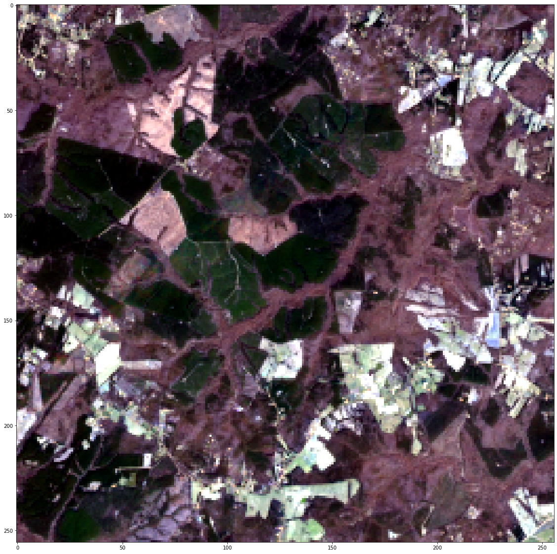
(a) Original image

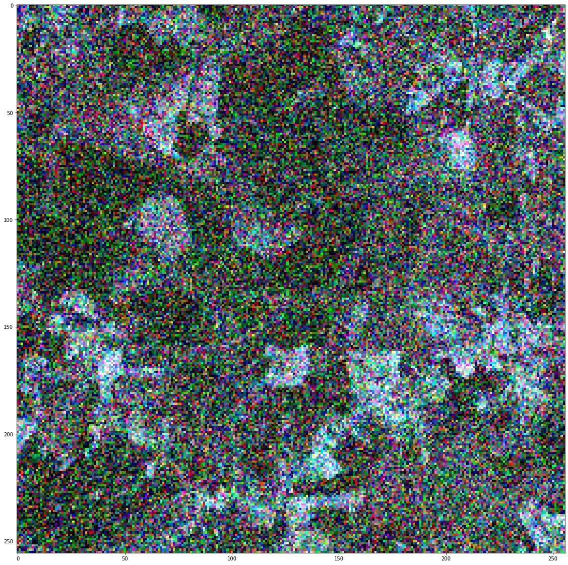
(b) Noisy image, $\sigma=0.04$

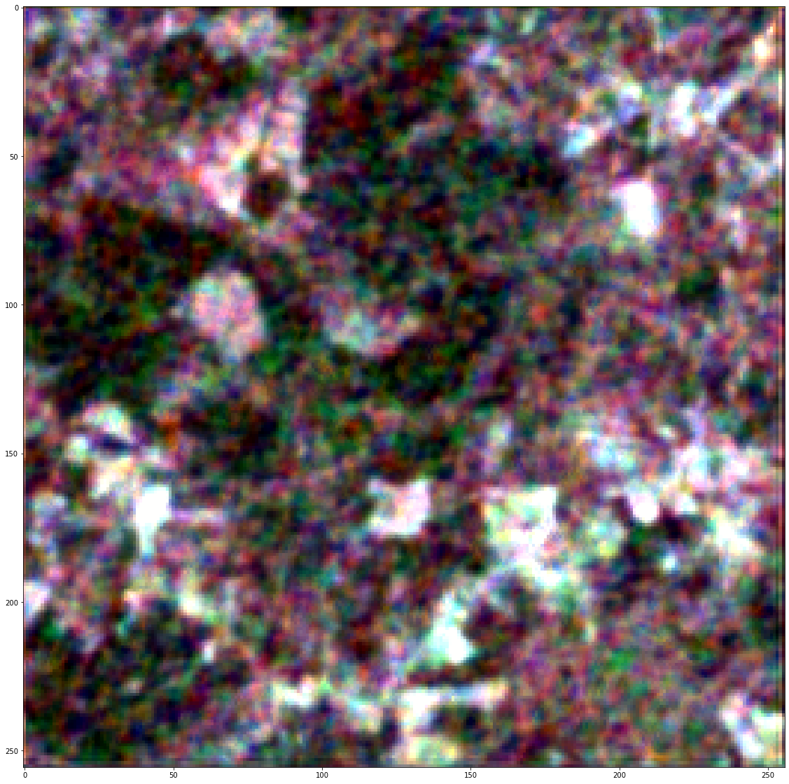
(c) RQUnet-VAE, $(\text{PSNR},\text{SSIM})=(38.502,0.966)$

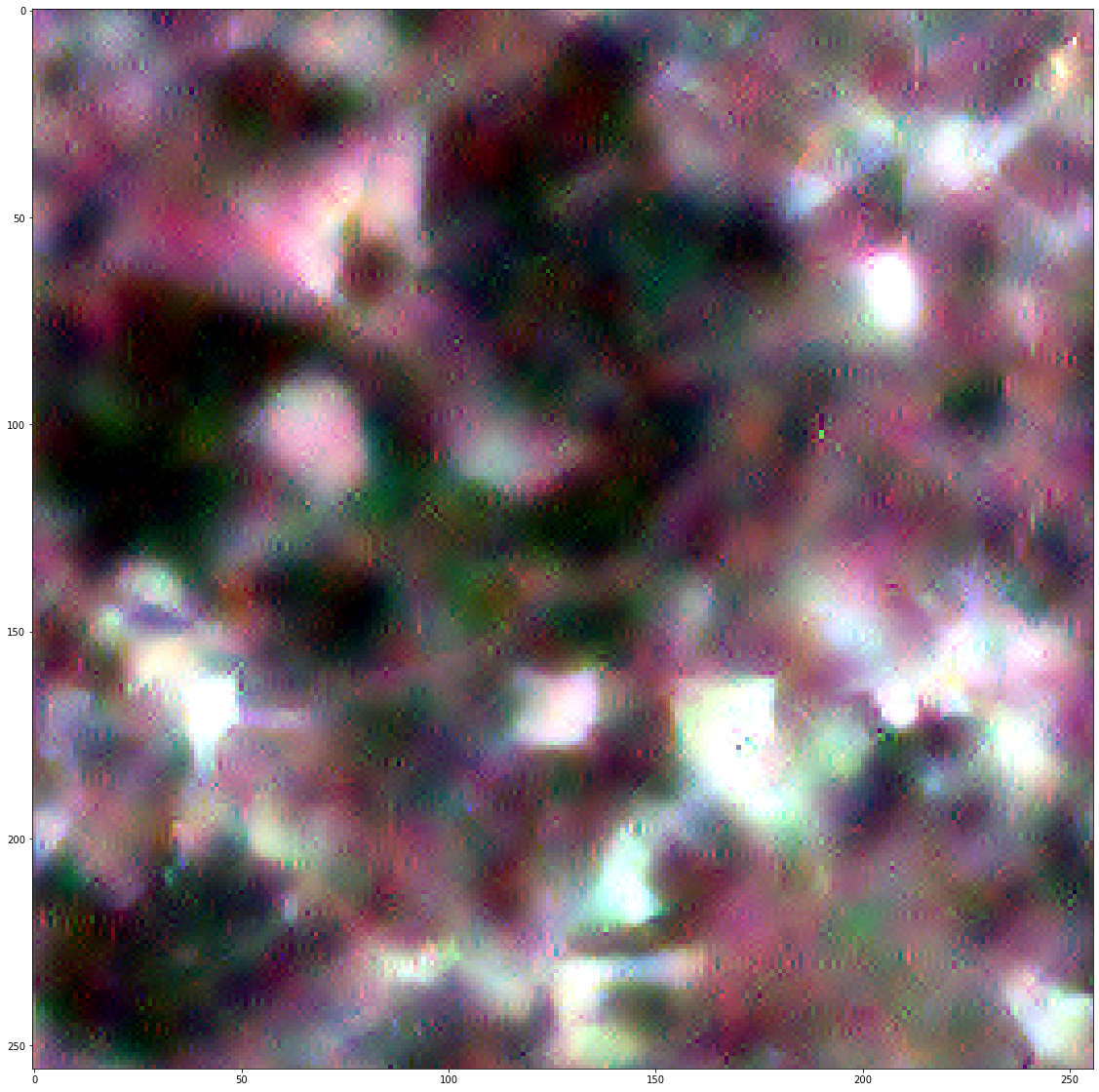
(d) Riesz Dyadic, $(\text{PSNR},\text{SSIM})=(37.555,0.96)$

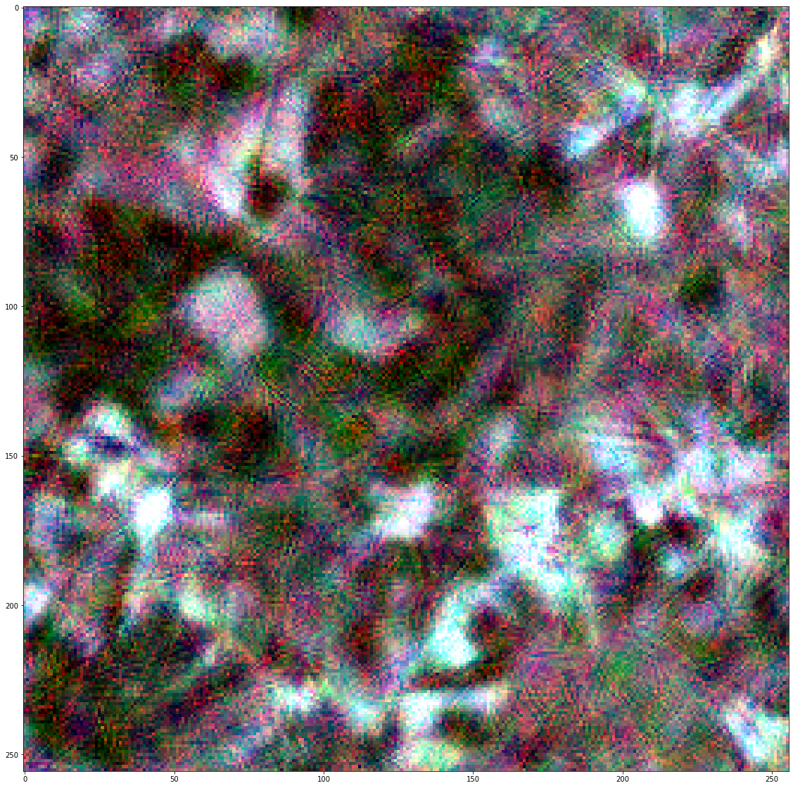
(e) curvelet, $(\text{PSNR},\text{SSIM})=(36.494,0.944)$

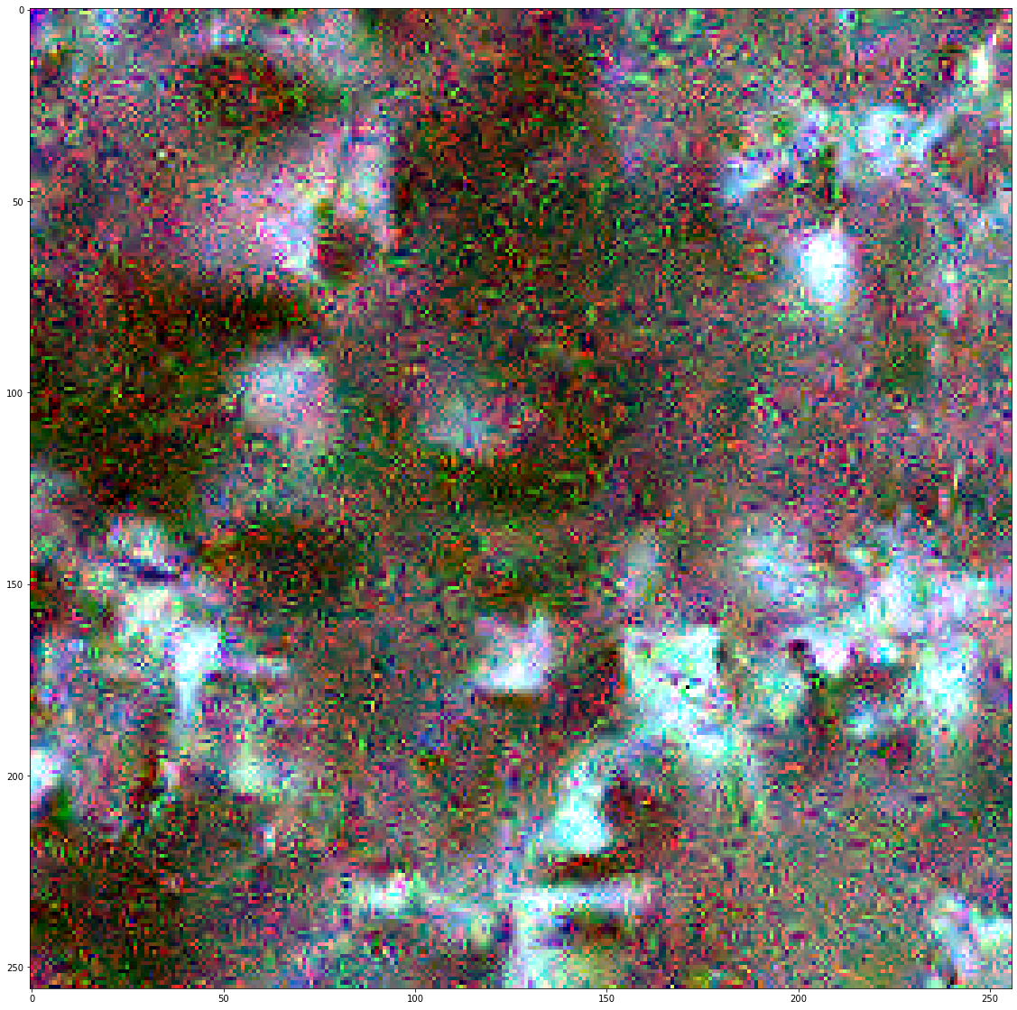
(f) wavelet CDF 9/7, $(\text{PSNR},\text{SSIM})=(35.646,0.936)$

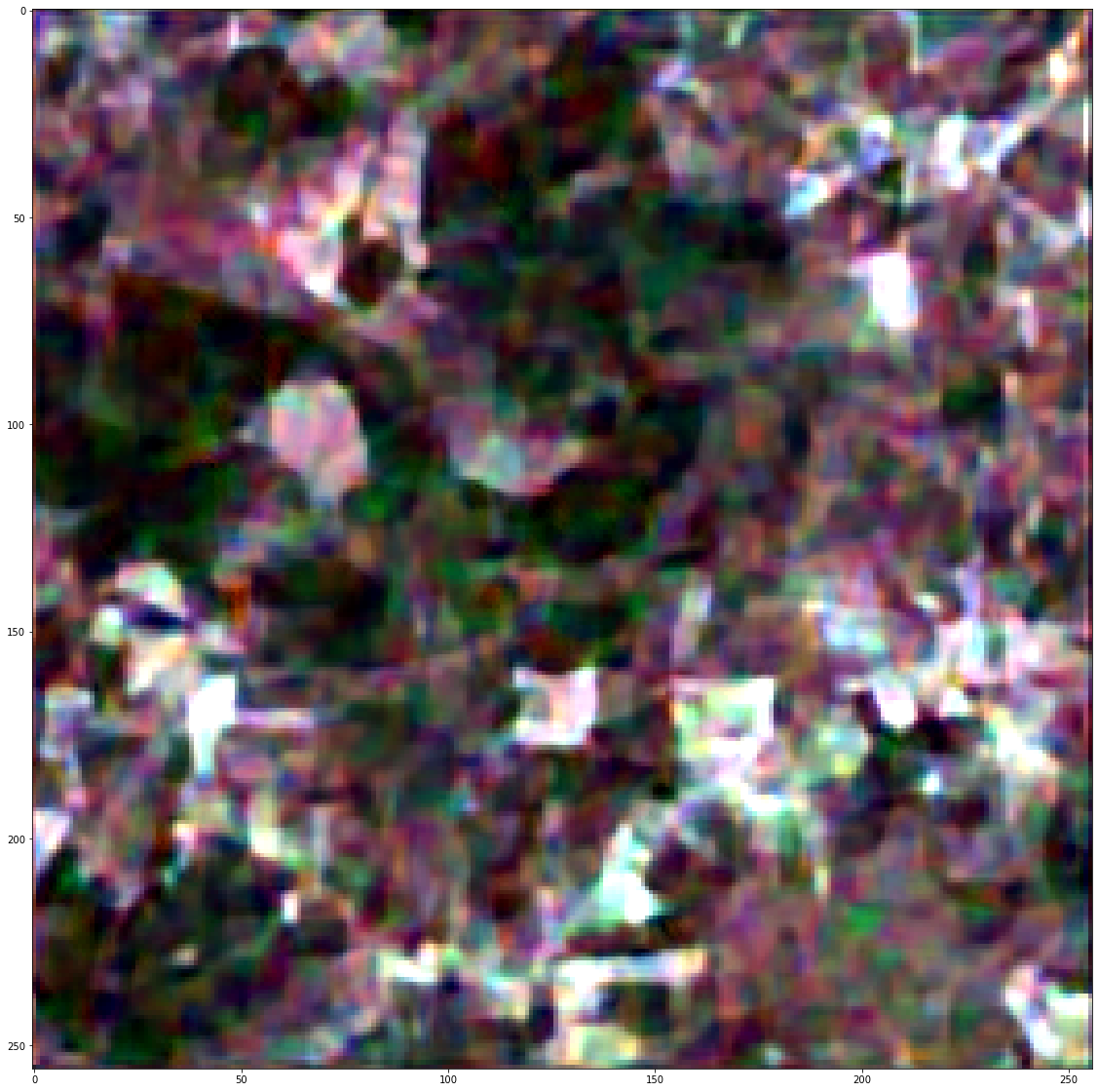
(g) RQUnet-VAE scheme 3, $(\text{PSNR},\text{SSIM})=(38.822,0.97)$

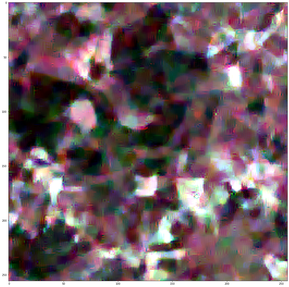
(h) GIAF-Riesz Dyadic, $(\text{PSNR},\text{SSIM})=(38.936,0.97)$

(i) TV-L2 $L=2$, $(\text{PSNR},\text{SSIM})=(38.513,0.967)$

(j) TV-L2 $L=9$, $(\text{PSNR},\text{SSIM})=(38.535,0.966)$

Figure 2: Qualitative image denoising results for RQUnet-VAE and competitor approaches. Image denoising by the RQUnet-VAE with standard deviation $\sigma=0.04$ and optimal $\alpha^{*}$.

III-B Denoising Experiments

To impose artificial noise on images for evaluation, Gaussian noise was added to each band of the Sentinel-2 images with a standard deviation of $\text{std}=0.04$. All images were normalized to interval $[0\,,1]$ using the image minimum and maximum. To give some examples, original image shown in Figure 2(a) and the corresponding image with added noise in Figure 2(b). (All ten test images with added noise are visualized in SM).

III-B1 Quantitative Results

Table I provides the results of the comparison of the RQUNet-VAE Schemes 1 and 2 with the state-of-the-art methods described in Section III-A2 using the evaluation metrics described in Section III-A3. For the ten test images described in Section III-A1 the proposed RQUNet-VAE Scheme 2 yields the highest Peak-Signal-to-Noise-Ratio (PSNR) and the highest Structural Similarity Index (SSIM) of all competitors (Table 1). Among all the approaches based on harmonic analysis, RQUNet-VAE Scheme 1 yields the best results. Note GIAF also iteratively computes scaling and wavelet coefficients, similar to our RQUNet-VAE Scheme 2. The main difference, however, is that GIAF employs Riesz Dyadic wavelet kernel for scaling and wavelet functions whereas RQUNet-VAE Scheme 2 uses our adapted RQUNet-VAE. Using this scheme, allows more redundant parameters to better learn specific features from the data and thus, better adapt to specific images. (Denoising results for all other test images are visualized in SM).

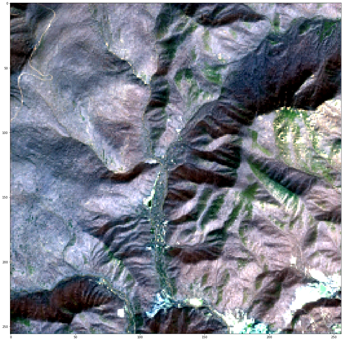
(a) Original image

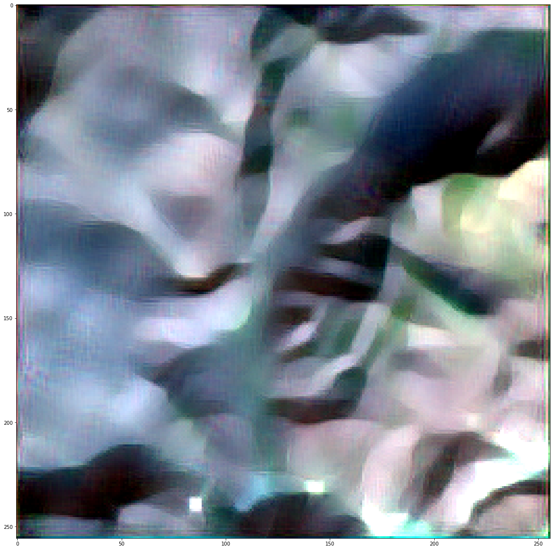
(b) Lowpass image

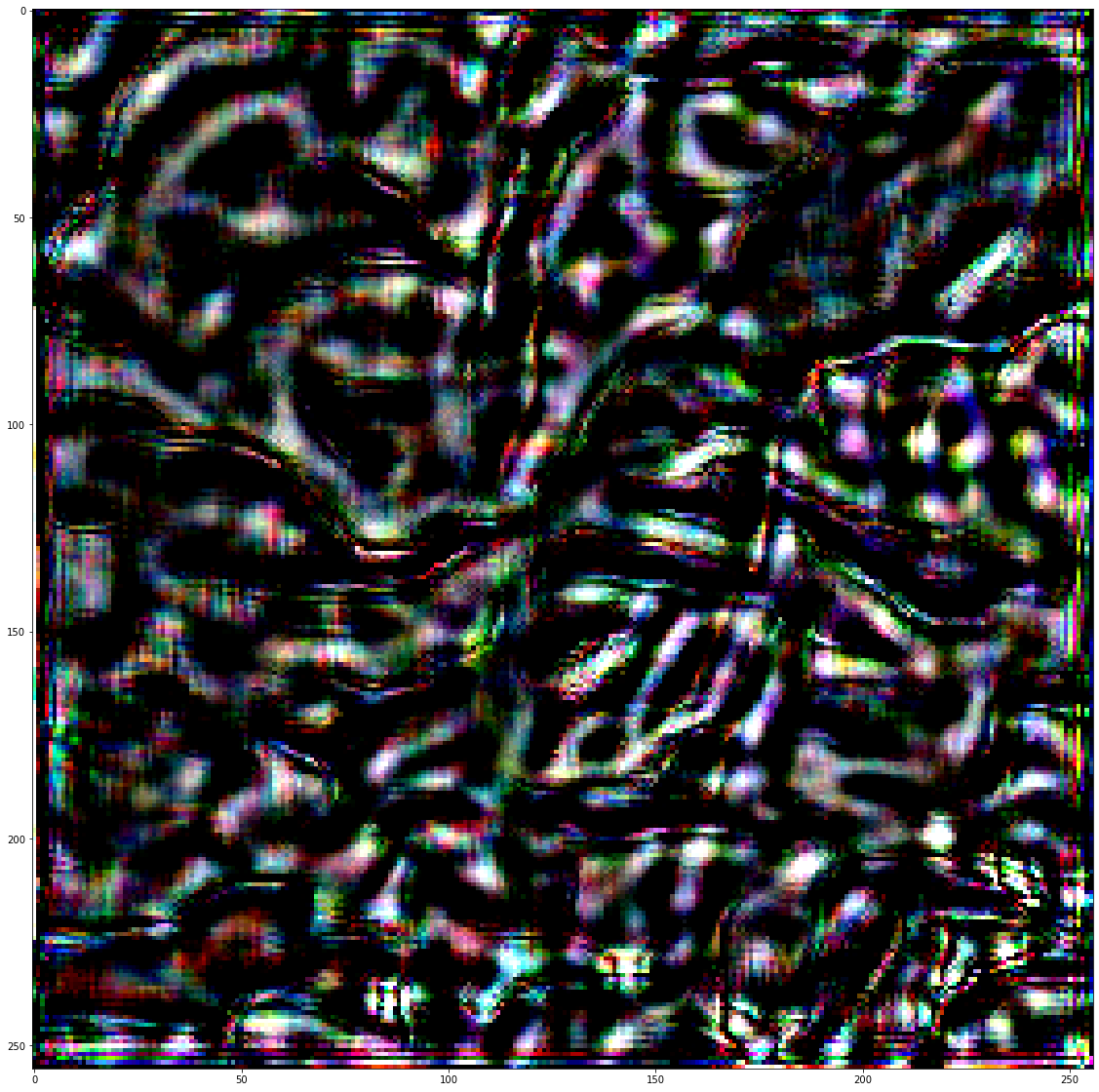
(c) Bandpass image

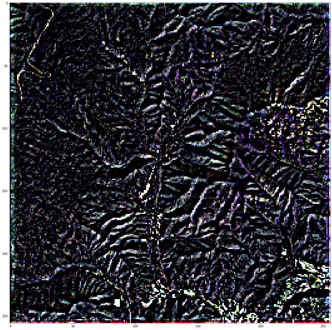
(d) Highpass image

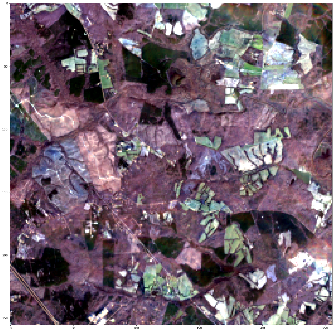
(e) Original image

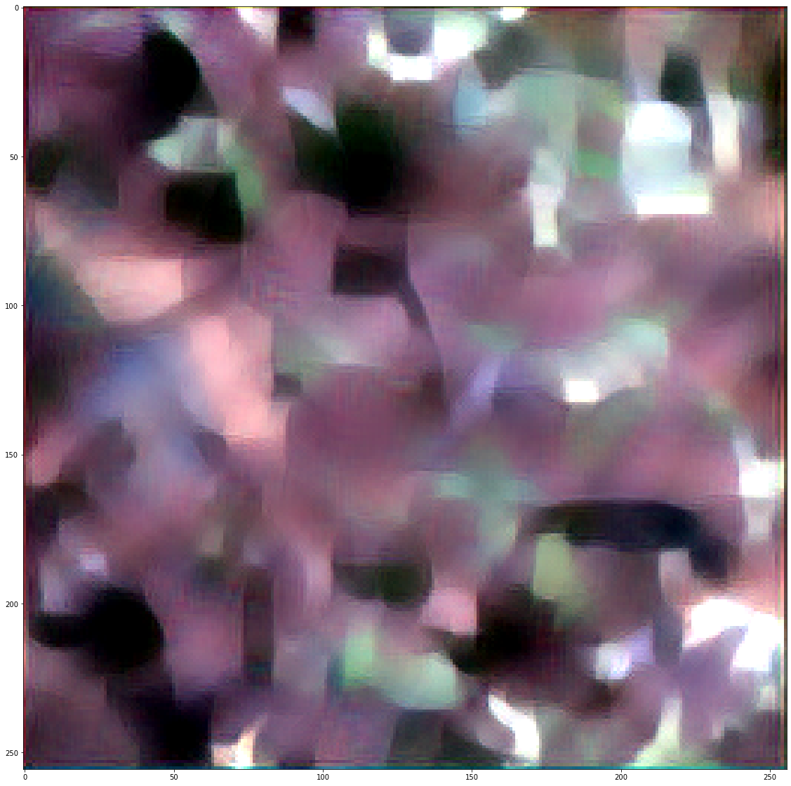
(f) Lowpass image

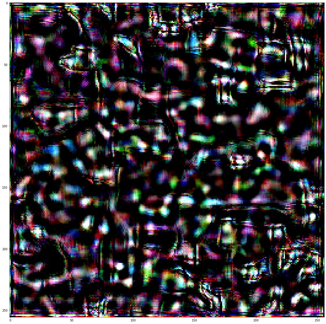
(g) Bandpass image

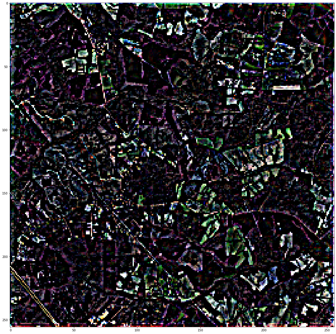
(h) Highpass image

Figure 3: Image decomposition by RQUNet-VAE by spectral analysis with a threshold $T=3$ for spectral histogram. Parameters: number of iteration $\text{Iter}=30$, a smoothing parameter $\alpha=0.4$.

III-B2 Qualitative Results

Figures 1, 2 and 3 in SM are original, noisy and denoised images with the 2nd scheme of our RQUNet-VAE. Figures 2(c)-2(j) provide qualitative results to assess how well the RQUNet-VAE schemes are able to reduce artificially added noise individual Sentinel2 images. Figure 2(c) shows the result of denoising the noisy image of Figure 2(b) using our RQUNet-VAE Scheme 1. Since Scheme 1 is based on harmonic analysis, we compare it to noise reduction using a Riesz Dyadic wavelet kernel [23] in Figure 2(d), using curvelets [3] in Figure 2(e), and using wavelet CDF 9/7 [33, 30, 6] in Figure 2(f). The RQUNet-VAE Scheme 1 best preserves the edges of objects of the original image. The Riez Dyadic wavelet kernel in Figure 2(d) yields a blurred denoised image. In contrast, wavelets (Figure 2(f)) better retain edges, but much of the noise remains. Across all these figures, it is clearly discernible that the proposed RQUNet-VAE Scheme 1 provides the best combination of noise reduction and delineation of edges and objects.

Figure 2(g) shows the denoised image using the RQUNet-VAE Scheme 2, compared to other iterative methods including GIAF [23] in Figure 2(h) and directional TV-L2 [27, 10, 31] using a number of directions $L=2$ in Figure 2(i) and $L=9$ in Figure 2(j). Figure 2 (g) illustrates that RQUNet-VAE significantly reduces artefacts while preserving texture pattern, contrast and sharp edges of objects in the reconstructed image, such that it is most similar to the original image. Note that the GIAF-Riesz dyadic method in Figure 2 (h) also performs very well, but a reconstructed images also contained some artefacts. The RQUNet-VAE Scheme 2 again provides the best trade-off between reduction of noise and delineation of edges and objects, where GIAF (Figure 2(h)) oversmoothes edges between objects while TV-L2 (Figure 2(i) and Figure 2(j)) still retain clearly visible noise. This demonstrates that the RQUNet-VAE with learned and deterministic frames increases sparsity in a generalized Besov space. Section III-D will demonstrate how this balance of noise reduction and discrimination of edges improves machine learning results when applying the RQUNet-VAE to segmentation of high resolution images for land cover mapping.

III-C Image Decomposition Experiments

This section evaluates how RQUNet-VAE Scheme 2 decomposes and subsequently denoises images. RQUNet-VAE Scheme 2 uses an iterative scheme to decompose an image into (i) a lowpass image, (ii) a bandpass image, and (iii) a highpass image. Denoising can be achieved by truncating highpass features. The RQUNet-VAE was applied to the Sentinel-2 image dataset described in Section III-A1. Figure 3 shows examples of the decomposition for four images. Figures 3(a,e) shows the original Sentinel2 images of a typical rural landscape with forest cover, cultivated fields and small, distributed structures. The corresponding lowpass images in Figures 3(b,f) captures the larger land cover parcels, without the fine-scale texture which has been removed. The corresponding bandpass in Figures 3(c,g) captures most of the signal of texture, whereas the highpass image in Figure Figures 3(d,h) captures very fine-scale texture, oscillating patterns, along with noise.

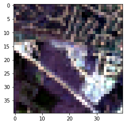
(a) Original frame 1

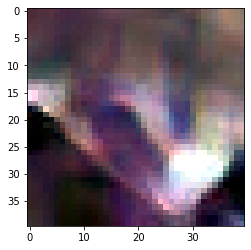
(b) Lowpass

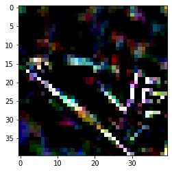
(c) Bandpass

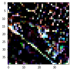
(d) Highpass

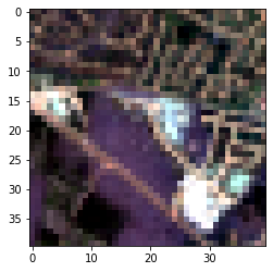
(e) Original frame 30

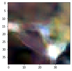
(f) Lowpass

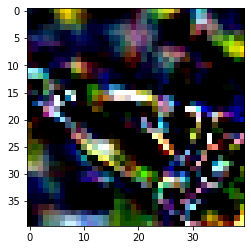
(g) Bandpass

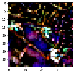
(h) Highpass

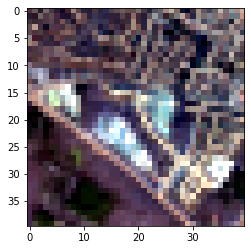
(i) Original frame 60

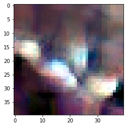
(j) Lowpass

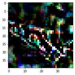
(k) Bandpass

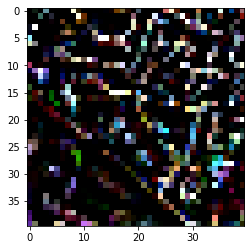
(l) Highpass

Figure 4: Time series decomposition by RQUNet-VAE with GIAF based spectral decomposition for site 296.

Time series decomposition

The RQUNet-VAE was applied to a Sentinel2 time series decomposition by using Haar wavelet smoothing in time as a diffusion process, (Section II-E). The proposed smoothing technique is therefore simultaneously applied in spatial domain (by RQUNet-VAE) and temporal domain (by Haar wavelet in time), following Algorithm 2 in SM. The smoothing parameter was set at $\alpha=0.03$ for all decompositions.

The Sentinel2 time series was comprised as follows: $\left\{\underline{\underline{\underline{f_{i}}}}\right\}_{i=1}^{80}$, $\underline{\underline{\underline{f_{i}}}}\in\mathbb{R}^{40\times 40\times 3\times 99}$, where each of the 99 images have three channels of image size $40\times 40$. The time series is then padded to $\underline{\underline{\underline{f_{i}}}}\in\mathbb{R}^{64\times 64\times 3\times 120}$. The RQUNet-VAE is trained on each image in the padded dataset to obtain all unknown model parameters. An Adam optimizer was used to train RQUNet-VAE with 200 epochs and batch-size of 16.

The trained parameters are then applied to Algorithm 2 with 10 iterations for spectral decomposition. Note that Algorithm 2 is an extension of generalized intersection algorithms with fixpoints [23] for video processing via spectral decomposition into lowpass, bandpass and highpass videos.

Figure 4 illustrates the time series decomposition with the RQUNet-VAE and diffusion process. The smoothing parameter was set at $\alpha=0.03$ for all decompositions. Similar to image decomposition in the previous sections, this time series decomposition extracts a homogeneous time series and a residual time series which contains small objects (e.g. roads), noise, and texture.

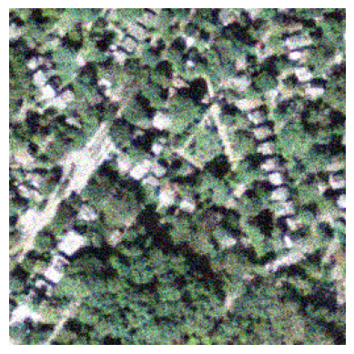
(a) Noisy image 1

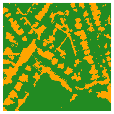
(b) Ground truth

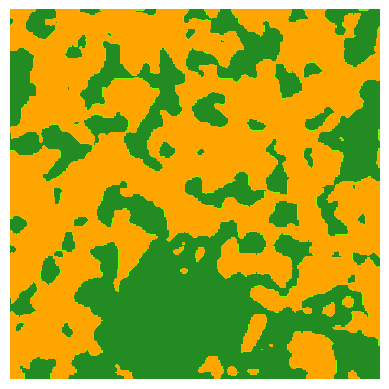
(c) RQUNet-VAE

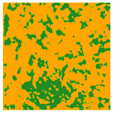
(d) Typical UNet

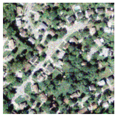
(e) Noisy image 2

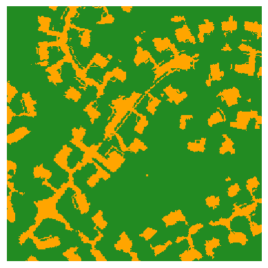
(f) Ground truth

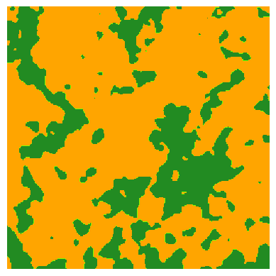
(g) RQUNet-VAE

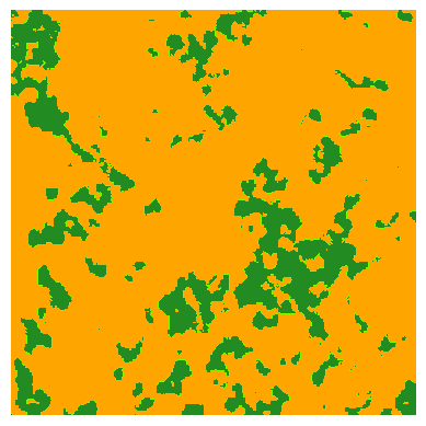
(h) Typical UNet

Figure 5: Segmentation result with RQUNet-VAE as a smoothing term for noisy images. a,e) NAIP images with artificial noise added ($\text{std}=0.08$) as input to segmentation; b,f) ground-truth segmentation masks; (c,g) segmentation masks returned by our RQUNet-VAE with a smoothing parameter $\alpha=0.5$; (d,h) segmentation mask returned by the typical UNet architecture [24].

III-D Image Segmentation by RQUNet-VAE 

The RQUNet-VAE was applied to the task of high resolution aerial image segmentation. The goal is to demonstrate that the RQUNet-VAE makes the image segmentation more robust to noise compared to the existing U-Net architecture. We first provide a brief background to the problem of image segmentation in Section III-D1. Then, in Section III-D2 we apply 1) the traditional U-Net architecture and 2) the RQUNet-VAE to the problem of image segmentation and show that RQUNet-VAE yields better segmentation results where artificial noise is added to images. This shows that our proposed RQUNet-VAE makes the existing U-Net architecture more robust to noise.

III-D1 Background on Image Segmentation

The conventional image segmentation procedure has the following steps, (i) pre-processing to remove noise and unwanted small objects, (ii) segmentation, (iii) post-processing with morphological operators. This 3-step process requires a large number of parameters that need to be selected by an expert. Therefore, attempts have been made to incorporate a smoothing term into various models. The Mumford-Shah model [17] was proposed to introduce a smoothing term in a minimization approach for segmentation. However, computation of this smoothing term is an NP-hard problem and therefore not feasible [17]. Later, the Chan-Vese segmentation model [4] was proposed that was solvable by relying on the level set method [19]. By adding a smoothing term in a variational formulae, this model successfully segments objects in a noisy background. Inspired by Chan-Vese model [4], we use RQUNet-VAE for segmentation by introducing a smoothing term, i.e. Riesz-Quincunx wavelet truncation, directly into the UNet-VAE. The advantage is that the RQUNet-VAE includes the smoothing term inside the Unet and thus combines (1) the ability of a Unet to learn features from an image, with (2) denoising capabilities enabled by the Riesz-Quincunx wavelet truncation. This smoothing term should eliminate small scale objects in a segmented image, e.g. texture and noise. Then, there is no need for separate pre- or post-processing steps, as these are all performed by the RQUNet-VAE segmentation.

TABLE II: Quantitative Comparison between RQUNet-VAE and the traditional UNet architecture. Since RQUNet-VAE uses a variational (non-deterministic) approach, we provide mean and standard deviation aggregated over 20 runs. Precision, recall, and F1-Score are provided for both classes [vegetated, impervious].

Algorithm	Accuracy	Precision	Recall	F1-Score
	(overall)	(per class)	(per class)	(per class)
RQUNet-VAE Mean (Image 1)	0.7057	[0.9047 0.4498]	[0.5457 0.8660]	[0.6807 0.5921]
RQUNet-VAE Stdev (Image 1)	$\pm$0.0013	$\pm$[0.0008 0.0014]	$\pm$[0.0030 0.0016]	$\pm$[0.0024 0.0012]
Traditional UNet (Image 1)	0.6640	[0.9460 0.3960]	[0.3780 0.9500]	[0.5400 0.5590]
RQUNet-VAE Mean (Image 2)	0.6734	[0.9837 0.3258]	[0.3662 0.9806]	[0.5337 0.4890]
RQUNet-VAE Stdev (Image 2)	$\pm$0.0012	$\pm$[0.0006 0.0009]	$\pm$[0.0027 0.0007]	$\pm$[0.0028 0.0010]
Traditional UNet (Image 2)	0.6170	[0.9860 0.2900]	[0.2440 0.9890]	[0.3920 0.4490]

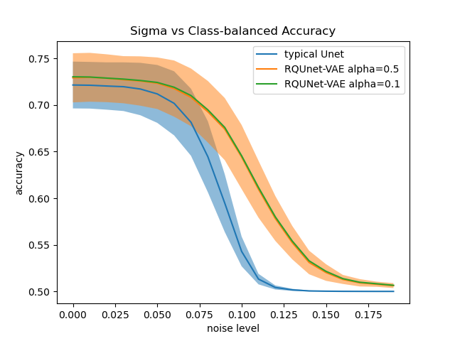
Figure 6: Outcome of segmentation experiments using the RQUNet-VAE and traditional UNet applied to 20 NAIP images with increasing added noise (0-0.20). The confidence intervals (blue and orange bands) are calculated from the mean and standard deviation of accuracy of 50 prediction iterations for each noise level and alpha value (0.5, 0.1) in the RQ scheme. This illustrates the results of variational terms of RQUNet-VAE.

III-D2 Experimental Evaluation of RQUNet-VAE for Image Segmentation

We apply both 1) the traditional U-Net [24] and 2) RQUNet-VAE to the problem of segmentation using the 20 NAIP images described in Section III-A1 using two classes of land cover, impervious and vegetated. Figure 5 shows the segmentation results for two sample images after noise has been added (Section III-B, standard deviation of $0.08$). The corresponding ground truth land cover masks are shown in Figures 5(b) and 5(f). Table II provides quantitative segmentation results, including overall accuracy, precision, recall, and F1-score for both of the two classes. Due to the added noise, the segmentation accuracy of the U-Net is very low at $0.6640$ and $0.6170$ for the two images, respectively Table II. The precision and recall for the two classes (non-impervious and impervious), indicate that this low accuracy is attributed to a bias towards the impervious class, as suggested by the low recall for the non-impervious class (0.3780 for the traditional UNet). This implies that more than two out of five impervious pixels are incorrectly classified as vegetated.

The performance of the traditional UNet is much lower with the added noise than on the original, which indicates that the addition of the noise substantially confuses the U-Net. In contrast, the RQUNet-VAE coped much better with the noise, yielding higher accuracy values of $0.7057\pm 0.0013$ and $0.6634\pm 0.0012$ for the two images, respectively. The negative impact of noise on the segmentation accuracy is substantially reduced when using the RQUNet-VAE which makes the U-Net more robust to noise. Furthermore, the RQUNet-VAE is better able to discriminate the vegetated class, shown by the higher F1-scores Table II.

A more comprehensive evaluation of RQUNet-VAE vs U-Net on 20 images with various levels of noise is given in Figure 6. This figure shows the mean accuracy (solid line) of the U-Net and the RQUNet-VAE across all 20 images. When using the original image with no noise ($\sigma=0$), the RQUNet-VAE only provides a marginal improvement over U-Net. As the noise level $\sigma$ is increased, both RQUNet-VAE and U-Net exhibit a drop in accuracy. However, that the drop in accuracy is substantially slower for RQUNet-VAE . In particular, for noise values around $\sigma=0.1$, the RQUNet-VAE has up to 10% higher accuracy than U-Net. This improvement stems from the variational auto-encoder approach, which, through variational changes to the latent representation of an image, allows the identification of pixels with a high probability of belonging to one class while being assigned to another class by the deterministic U-Net. Figure 6 gives the results using two parameters setting of RQUNet-VAE , $\alpha=0.5$ and $\alpha=1.0$. In both cases the resulting accuracy is nearly identical (the two lines are almost perfectly on top of each other), showing that the the performance is not very sensitive to the choice of $\alpha$ and thus that RQUNet-VAE is robust to non-optimal choices of $\alpha$. In summary, Figure 6 shows that our proposed RQUNet-VAE is much more robust to Gaussian noise added to an image, as the reduction of segmentation accuracy with higher noise levels, is less pronounced.

IV Conclusion

In this work, we introduced the RQUNet-VAE which augments the existing UNet architecture with a generalized wavelet expansion approach that we extended to a diffusion process to enable spectral decomposition. To the best of our knowledge this is the first approach that enables image decomposition and image denoising using a variational variant of the UNet architecture. An important application of this decomposition is denoising, achieved by truncating highpass features, that is, discarding information of decomposed images having the highest variance. We apply our proposed RQUNet-VAE to image denoising and segmentation of multi-band satellite images and their time-series which often contain noise due to multiple causes. During quantitative comparisons of noise reduction the RQUNet-VAE yields the highest PSNR and SSIM of all competitor methods. Among all the approaches based on harmonic analysis, RQUNet-VAE Scheme 2 yields the best results. For the application of satellite image denoising our proposed RQUNet-VAE provides superior qualitative performance compared to other competitors. The denoising by RQUNet-VAE Scheme 1 was visually compared to the noise reduction using a Riesz Dyadic wavelet and curvelets and using wavelet CDF and it provided the best combination of noise reduction and delineation of edges and objects. Furthermore the propose RQUNet-VAE Scheme 2, was compared to other iterative methods including GIAF and directional TV-L2 and it resulted in the best trade-off between reduction of noise and delineation of edges and objects, whereas the GIAF oversmoothed edges between objects while TV-L2 clearly retained visible noise.

To quantitatively measure the improvement of the RQUNet-VAE against the traditional UNet, we applied it to high resolution aerial image segmentation. Our experiments show only a slight improvement over the traditional UNet for segmantation of the original images with little noise. However, as artificial noise is added to images, we observe that the segmentation quality of the UNet decreases more rapidly than when using the RQUNet-VAE . The superior performance of RQUNet-VAE is due to a neural network in UNet-VAE with a learned dictionary obtained from the training procedure to increase the level of sparsity for an input image in a generalized Besov space. This property is due to a fundamental concept in signal processing, that the signal is sparse in some transformed domain. This demonstrates that the RQUNet-VAE architecture is able to substantially increase the robustness to noise compared to the traditional UNet for the application of satellite image segmentation.

V Acknowledgments

This research is based upon work supported in part by the Office of the Director of National Intelligence (ODNI), Intelligence Advanced Research Projects Activity (IARPA), Space-based Machine Automated Recognition Technique (SMART) program, via contract 2021-20111000003. The views and conclusions contained herein are those of the authors and should not be interpreted as necessarily representing the official policies, either expressed or implied, of ODNI, IARPA, or the U.S. Government. The U.S. Government is authorized to reproduce and distribute reprints for governmental purposes notwithstanding any copyright annotation therein. The research was conducted in collaboration with BlackSky. We thank Diego Torrejon and Isaac Corley of BlackSky for valuable comments on the manuscript.

References

• [1] J. Allenby and C. Phelan. Implementing technology and precision conservation in the Chesapeake bay. Chesapeake Conservancy, 2013.
• [2] J.-F. Cai, R. H. Chan, and Z. Shen. A framelet-based image inpainting algorithm. Applied and Computational Harmonic Analysis, 24(2):131–149, 2008.
• [3] E. J. Candès and D. L. Donoho. New tight frames of curvelets and optimal representations of objects with piecewise c2 singularities. Communications on Pure and Applied Mathematics: A Journal Issued by the Courant Institute of Mathematical Sciences, 57(2):219–266, 2004.
• [4] T. F. Chan and L. A. Vese. Active contours without edges. IEEE Transactions on image processing, 10(2):266–277, 2001.
• [5] M. Claverie, J. Ju, J. G. Masek, J. L. Dungan, E. F. Vermote, J.-C. Roger, S. V. Skakun, and C. Justice. The harmonized Landsat and Sentinel-2 surface reflectance data set. Remote sensing of environment, 219:145–161, 2018.
• [6] I. Daubechies and W. Sweldens. Factoring wavelet transforms into lifting steps. Journal of Fourier analysis and applications, 4(3):247–269, 1998.
• [7] P. Esser, E. Sutter, and B. Ommer. A variational U-Net for conditional appearance and shape generation. In Proceedings of the IEEE conference on computer vision and pattern recognition, pages 8857–8866, 2018.
• [8] M. Feilner, D. Van De Ville, and M. Unser. An orthogonal family of Quincunx wavelets with continuously adjustable order. IEEE Transactions on Image Processing, 14(4):499–510, 2005.
• [9] G. Gilboa. A total variation spectral framework for scale and texture analysis. SIAM journal on Imaging Sciences, 7(4):1937–1961, 2014.
• [10] T. Goldstein and S. Osher. The split Bregman method for $\text{L}_{1}$-regularized problems. SIAM journal on imaging sciences, 2(2):323–343, 2009.
• [11] S. Ioffe and C. Szegedy. Batch normalization: Accelerating deep network training by reducing internal covariate shift. In International conference on machine learning, pages 448–456. PMLR, 2015.
• [12] D. P. Kingma and J. Ba. Adam: A method for stochastic optimization. arXiv preprint arXiv:1412.6980, 2014.
• [13] D. P. Kingma and M. Welling. Auto-encoding variational bayes. arXiv preprint arXiv:1312.6114, 2013.
• [14] W. Kleynhans, B. P. Salmon, J. C. Olivier, F. Van den Bergh, K. J. Wessels, T. L. Grobler, and K. C. Steenkamp. Land cover change detection using autocorrelation analysis on MODIS time-series data: Detection of new human settlements in the gauteng province of south africa. IEEE Journal of selected topics in applied earth observations and remote sensing, 5(3):777–783, 2012.
• [15] S. Kohl, B. Romera-Paredes, C. Meyer, J. De Fauw, J. R. Ledsam, K. Maier-Hein, S. Eslami, D. Jimenez Rezende, and O. Ronneberger. A probabilistic U-Net for segmentation of ambiguous images. Advances in neural information processing systems, 31, 2018.
• [16] J. Li and D. P. Roy. A global analysis of Sentinel-2A, Sentinel-2B and Landsat-8 data revisit intervals and implications for terrestrial monitoring. Remote Sensing, 9(9):902, 2017.
• [17] D. B. Mumford and J. Shah. Optimal approximations by piecewise smooth functions and associated variational problems. Communications on pure and applied mathematics, 1989.
• [18] NAIP. National agriculture imagery program (NAIP) information sheet, 2015. https://www.fsa.usda.gov/Internet/FSA_File/naip_info_sheet_2015.pdf.
• [19] S. Osher and J. A. Sethian. Fronts propagating with curvature-dependent speed: Algorithms based on hamilton-jacobi formulations. Journal of computational physics, 79(1):12–49, 1988.
• [20] J. R. Partington, J. R. Partington, et al. An introduction to Hankel operators. Cambridge University Press, 1988.
• [21] N. G. Polson, J. G. Scott, and B. T. Willard. Proximal algorithms in statistics and machine learning. Statistical Science, 30(4):559–581, 2015.
• [22] Y. Pu, Z. Gan, R. Henao, X. Yuan, C. Li, A. Stevens, and L. Carin. Variational autoencoder for deep learning of images, labels and captions. Advances in neural information processing systems, 29, 2016.
• [23] R. Richter, D. H. Thai, and S. F. Huckemann. Generalized intersection algorithms with fixpoints for image decomposition learning. CoRR, abs/2010.08661, 2020.
• [24] O. Ronneberger, P. Fischer, and T. Brox. U-net: Convolutional networks for biomedical image segmentation. In International Conference on Medical image computing and computer-assisted intervention, pages 234–241. Springer, 2015.
• [25] D. P. Roy, H. Huang, L. Boschetti, L. Giglio, L. Yan, H. H. Zhang, and Z. Li. Landsat-8 and Sentinel-2 burned area mapping-A combined sensor multi-temporal change detection approach. Remote Sensing of Environment, 231:111254, 2019.
• [26] D. P. Roy, Y. Jin, P. Lewis, and C. Justice. Prototyping a global algorithm for systematic fire-affected area mapping using MODIS time series data. Remote sensing of environment, 97(2):137–162, 2005.
• [27] L. I. Rudin, S. Osher, and E. Fatemi. Nonlinear total variation based noise removal algorithms. Physica D: nonlinear phenomena, 60(1-4):259–268, 1992.
• [28] B. P. Salmon, W. Kleynhans, F. Van den Bergh, J. C. Olivier, T. L. Grobler, and K. J. Wessels. Land cover change detection using the internal covariance matrix of the extended Kalman filter over multiple spectral bands. IEEE Journal of selected topics in applied earth observations and remote sensing, 6(3):1079–1085, 2013.
• [29] N. Srivastava, G. Hinton, A. Krizhevsky, I. Sutskever, and R. Salakhutdinov. Dropout: a simple way to prevent neural networks from overfitting. The journal of machine learning research, 15(1):1929–1958, 2014.
• [30] W. Sweldens. The lifting scheme: A construction of second generation wavelets. SIAM journal on mathematical analysis, 29(2):511–546, 1998.
• [31] D. H. Thai and C. Gottschlich. Directional global three-part image decomposition. EURASIP Journal on Image and Video Processing, 2016(1):1–20, 2016.
• [32] C. Tian, L. Fei, W. Zheng, Y. Xu, W. Zuo, and C.-W. Lin. Deep learning on image denoising: An overview. Neural Networks, 131:251–275, 2020.
• [33] M. Unser and T. Blu. Mathematical properties of the jpeg2000 wavelet filters. IEEE transactions on image processing, 12(9):1080–1090, 2003.
• [34] M. Unser, N. Chenouard, and D. Van De Ville. Steerable pyramids and tight wavelet frames in ${L}_{2}(\mathbb{R}^{d})$. IEEE Transactions on Image Processing, 20(10):2705–2721, Oct. 2011.
• [35] M. Unser, D. Sage, and D. Van De Ville. Multiresolution monogenic signal analysis using the Riesz-Laplace wavelet transform. IEEE Transactions on Image Processing, 18(11):2402–2418, Nov. 2009.
• [36] M. Unser and D. Van De Ville. Wavelet steerability and the higher-order Riesz transform. IEEE Transactions on Image Processing, 19(3):636–652, Mar. 2010.
• [37] F. Van Den Bergh, K. J. Wessels, S. Miteff, T. L. Van Zyl, A. D. Gazendam, and A. K. Bachoo. Hitempo: A platform for time-series analysis of remote-sensing satellite data in a high-performance computing environment. International Journal of Remote Sensing, 33(15):4720–4740, 2012.
• [38] T. Van Erven and P. Harremos. Rényi divergence and Kullback-Leibler divergence. IEEE Transactions on Information Theory, 60(7):3797–3820, 2014.
• [39] E. Vermote, C. Justice, M. Claverie, and B. Franch. Preliminary analysis of the performance of the Landsat 8/OLI land surface reflectance product. Remote Sensing of Environment, 185:46–56, 2016.
• [40] M. Vetterli, P. Marziliano, and T. Blu. Sampling signals with finite rate of innovation. IEEE transactions on Signal Processing, 50(6):1417–1428, 2002.
• [41] Z. Wang and A. C. Bovik. Mean squared error: Love it or leave it? a new look at signal fidelity measures. IEEE signal processing magazine, 26(1):98–117, 2009.
• [42] C. E. Woodcock, T. R. Loveland, M. Herold, and M. E. Bauer. Transitioning from change detection to monitoring with remote sensing: A paradigm shift. Remote Sensing of Environment, 238:111558, 2020.
• [43] J. C. Ye, Y. Han, and E. Cha. Deep convolutional framelets: A general deep learning framework for inverse problems. SIAM Journal on Imaging Sciences, 11(2):991–1048, 2018.
• [44] R. Yin, T. Gao, Y. M. Lu, and I. Daubechies. A tale of two bases: Local-nonlocal regularization on image patches with convolution framelets. SIAM Journal on Imaging Sciences, 10(2):711–750, 2017.
• [45] H. K. Zhang, D. P. Roy, L. Yan, Z. Li, H. Huang, E. Vermote, S. Skakun, and J.-C. Roger. Characterization of Sentinel-2A and Landsat-8 top of atmosphere, surface, and nadir BRDF adjusted reflectance and NDVI differences. Remote sensing of environment, 215:482–494, 2018.
• [46] Z. Zhu. Change detection using Landsat time series: A review of frequencies, preprocessing, algorithms, and applications. ISPRS Journal of Photogrammetry and Remote Sensing, 130:370–384, 2017.