Kinematical higher-twist corrections in $\gamma^{*}\gamma\to\pi\pi$

Abstract

We apply the Braun-Manashov technique to improve the description of $\gamma^{*}(q_{1})\gamma(q_{2})\to M(p_{1})M(p_{2})$ amplitudes at large $Q^{2}=-q_{1}^{2}$ and small $s=(q_{1}+q_{2})^{2}$. We derive the kinematical higher-twist contributions of order $s/Q^{2}$ and $m^{2}/Q^{2}$ to the helicity amplitudes and estimate their sizes in the kinematics accessible at Belle and Belle II. Since pion GPDs cannot be directly measured by experiment, $\pi\pi$ GDAs are the best way to investigate the energy-momentum tensor form factors for pions.

I Introduction

Since generalized distribution amplitudes (GDAs) Muller:1994ses ; Diehl:1998dk ; Polyakov:1998ze are hadronic matrix elements of the same bilocal quark (or gluon) operator on the light-cone as the operator entering the definition of generalized parton distributions (GPDs) Diehl:2003ny , the techniques developed by Braun and Manashov  Braun:2011dg ; Braun:2011zr ; Braun:2011th to separate kinematical and dynamical contributions in the product of two electromagnetic currents $T\{j_{\mu}^{\text{em}}(z_{1}x)j_{\nu}^{\text{em}}(z_{2}x)\}$ and applied to the deeply-virtual Compton scattering (DVCS) reaction Braun:2012bg can be used in the description of the reaction

$$e(k_{1})\gamma\to e^{\prime}(k_{2})M_{1}(p_{1})M_{2}(p_{2})$$ (1)

accessible in $e^{+}e^{-}$ collisions. GDAs can be accessed in these reactions Diehl:2000uv in the kinematical range where $Q^{2}=-(k_{2}-k_{1})^{2}$ is large but $s=(p_{1}+p_{2})^{2}$ is much smaller than $Q^{2}$. They have already been the subject of careful studies at Belle Belle:2015oin ; Kumano:2017lhr .

The kinematical corrections considered here come from two types of operators, namely 1) the subtraction of traces in the leading-twist operators and 2) the higher-twist operators which can be reduced to the total derivatives of the leading-twist ones. The kinematical corrections in DVCS can be considered as a generalization of the target mass corrections in deep inelastic scattering Nachtmann:1973mr .

II Kinematics and generalized distribution amplitudes

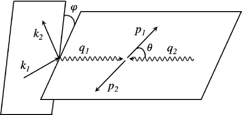
Figure 1: Kinematics of the process $\gamma^{*}(q_{1})\gamma(q_{2})\to\pi(p_{1})\pi(p_{2})$ in the center of mass of the meson pair; the virtual photon is emitted by the electron, $q_{1}=k_{1}-k_{2}$.

To describe the process (1), we define the lightlike vectors $n$ and $\tilde{n}$ as

$$\tilde{n}=q_{1}+(1-\tau)q_{2},\qquad n=q_{2},$$ (2)

where $\tau=s/(Q^{2}+s)$, $Q^{2}=-q_{1}^{2}$, and $s=(q_{1}+q_{2})^{2}=(p_{1}+p_{2})^{2}$. The polar angle of the meson ($M_{i}$) momenta $\theta$ is illustrated in Fig. 1 and defined as ($m$ is the mass of the meson):

$$\cos{\theta}=\frac{2q_{1}\cdot(p_{2}-p_{1})}{\beta_{0}\,(Q^{2}+s)},\qquad\beta_{0}=\sqrt{1-\frac{4m^{2}}{s}}.$$ (3)

The skewness variable

$$\zeta_{0}=\frac{(p_{2}-p_{1})\cdot n}{(p_{2}+p_{1})\cdot n},$$ (4)

is related to $\cos\theta$ through $\zeta_{0}=-\beta_{0}\cos{\theta}$. In our kinematics, only $\Delta=p_{2}-p_{1}$ has a transverse momentum, $\Delta=\zeta_{0}(\tilde{n}-\tau n)+\Delta_{T}$. Using the on-shell condition, $\Delta_{T}^{2}=4m^{2}-(1-\zeta_{0}^{2})s$.

The leading-twist amplitude was first presented in Ref. Diehl:2000uv with the help of a twist-2 GDA $\Phi(z,\zeta_{0},s)$ for an isoscalar meson pair,

$$\langle M(p_{2})M(p_{1})|\,O_{++}(z_{1}n,z_{2}n)\,|0\rangle=\chi\,2P\cdot n\int dz\,e^{2i\left[zz_{1}+(1-z)z_{2}\right]P\cdot n}\,\Phi(z,\zeta_{0},s),$$ (5)

where $P=(p_{1}+p_{2})/2$, $\chi=5e^{2}/18$ and $\Phi$ is the sum of GDAs of the quark flavors $u$ and $d$, $\Phi=\Phi_{u}+\Phi_{d}$. $O_{++}(z_{1}n,z_{2}n)$ is the leading-twist vector operator (a light-like Wilson line joining the points $z_{1}n$ and $z_{2}n$ is implied),

$$O_{++}(z_{1}n,z_{2}n)=\chi\left[\bar{u}(z_{1}n)\not{n}u(z_{2}n)+\bar{d}(z_{1}n)\not{n}d(z_{2}n)\right].$$ (6)

The matrix element of this operator can also be expressed in terms of double distributions as Teryaev:2001qm

$$\langle M(p_{2})M(p_{1})|\,O_{++}(z_{1}n,z_{2}n)\,|0\rangle=\chi\int d\beta\,d\alpha\left[f(\beta,\alpha)\,\Delta\cdot n-g(\beta,\alpha)\,2P\cdot n\right]e^{-il_{z_{1}z_{2}}\cdot n}$$ (7)

with $f$ and $g$ having support on the rhombus $|\alpha|+|\beta|\leq 1$ and assumed to vanish at the boundary, and

$$l_{z_{1}z_{2}}=(z_{2}-z_{1})\left[\beta\,\frac{\Delta}{2}-(\alpha+1)P\right]-2z_{1}P.$$ (8)

Then, setting $z_{1}-z_{2}=1$, one can easily relate the GDA to double distributions

$$\Phi(z,\zeta_{0},s)=2\int d\beta\,d\alpha\,\delta(y+\alpha-\beta\zeta_{0})\left[f(\beta,\alpha)\,\zeta_{0}-g(\beta,\alpha)\right],$$ (9)

where $y=2z-1$.

In general, GDAs can be expanded as Diehl:2000uv

$$\Phi(z,\cos\theta,s)=6z(1-z)\sum_{n=1,\text{odd}}^{\infty}\sum_{l=0,\text{even}}^{n+1}\tilde{B}_{nl}(s)C_{n}^{(3/2)}(2z-1)P_{l}(\cos\theta).$$ (10)

In the asymptotic limit ($Q^{2}\rightarrow\infty$), only the $n=1$ term survives,

$$\Phi(z,\cos\theta,s)=18z(1-z)(2z-1)\left[\tilde{B}_{10}(s)+\tilde{B}_{12}(s)P_{2}(\cos\theta)\right],$$ (11)

where the first and second terms indicate the S-wave and D-wave production of a meson pair, respectively.

III Helicity amplitudes

The amplitude for $\gamma^{*}\gamma\to MM$ reads,

$$A_{\mu\nu}=i\int d^{4}x\,e^{-ir\cdot x}\langle M(p_{2})M(p_{1})|\,T\{j_{\mu}^{\text{em}}(z_{1}x)j_{\nu}^{\text{em}}(z_{2}x)\}\,|0\rangle,\!\!$$ (12)

where $r=z_{1}q_{1}+z_{2}q_{2}$, and the constraint $z_{1}-z_{2}=1$ is imposed. Electromagnetic gauge invariance leads to the decomposition Braun:2012bg

$$A^{\mu\nu}=-A^{(0)}\,g_{\perp}^{\mu\nu}+A^{(1)}\,\frac{\Delta_{\alpha}g_{\perp}^{\alpha\nu}}{Q}\left(\tilde{n}^{\mu}+(1-\tau)n^{\mu}\right)+\frac{1}{2}\,A^{(2)}\,\Delta_{\alpha}\Delta_{\beta}(g_{\perp}^{\alpha\mu}g_{\perp}^{\beta\nu}-\epsilon_{\perp}^{\alpha\mu}\epsilon_{\perp}^{\beta\nu})+A^{(3)\mu}\,n^{\nu}$$ (13)

with $g_{\perp}^{\mu\nu}$ and $\epsilon_{\perp}^{\mu\nu}$ given by

$$g_{\perp}^{\mu\nu}=g^{\mu\nu}-\frac{n^{\mu}\tilde{n}^{\nu}+n^{\nu}\tilde{n}^{\mu}}{n\cdot\tilde{n}},\qquad\epsilon_{\perp}^{\mu\nu}=\epsilon^{\mu\nu\alpha\beta}\,\frac{\tilde{n}_{\alpha}n_{\beta}}{n\cdot\tilde{n}}.$$ (14)

The last term in Eq. (13) is of no interest since it does not contribute to any observable, and the rest of them can be expressed in terms of the GDAs if the factorization condition $Q^{2}\gg s,\Lambda_{\text{QCD}}^{2}$ is satisfied.

To calculate the helicity amplitudes, we define the photon polarization vectors as Diehl:2000uv

$$\epsilon_{0}^{\mu}=\frac{1}{Q}(|q_{1}^{3}|,0,0,q_{1}^{0}),\,\,\epsilon_{\pm}^{\mu}=\frac{1}{\sqrt{2}}(0,\mp 1,-i,0),$$ (15)

where the lower indices $\pm$ and $0$ indicate the helicities of the photon. The polarization vectors $\tilde{\epsilon}$ for the real photon only have the transverse components, and they are related to the ones of the virtual photon as $\tilde{\epsilon}_{\pm}=-\epsilon_{\mp}$. There are three independent helicity amplitudes $A_{ij}=\epsilon_{i}^{\mu}\tilde{\epsilon}_{j}^{\nu}A_{\mu\nu}.$ We choose the independent helicity amplitudes as $A^{(0)}=A_{++}$, $A_{0+}=-A^{(1)}(\Delta\cdot\epsilon_{-})$ and $A_{-+}=-A^{(2)}(\Delta\cdot\epsilon_{-})^{2}$.

We shall not detail here our calculation of the helicity amplitudes of $\gamma^{*}\gamma\to MM$; we adopt (and adapt to our case) the techniques used for the DVCS amplitude in Ref. Braun:2012bg . Our results for the helicity amplitudes in terms of GDAs read :

$$A^{(0)}= \chi\left\{(1-\frac{s}{2Q^{2}})\int_{0}^{1}dz\frac{\Phi(z,\eta,s)}{1-z}-\frac{s}{Q^{2}}\int_{0}^{1}dz\frac{\Phi(z,\eta,s)}{z}\ln(1-z)\right.$$

$$-\left.(\frac{2s}{Q^{2}}\eta+\frac{\Delta_{T}^{2}}{\beta_{0}^{2}Q^{2}}\frac{\partial}{\partial\eta})\frac{\partial}{\partial\eta}\int_{0}^{1}dz\frac{\Phi(z,\eta,s)}{z}\left[\frac{\ln(1-z)}{2}+Li_{2}(1-z)-Li_{2}(1)\right]\right\},$$

$$A^{(1)}= \frac{2\chi}{\beta_{0}Q}\frac{\partial}{\partial\eta}\int_{0}^{1}dz\Phi(z,\eta,s)\frac{\ln(1-z)}{z},$$

$$A^{(2)}= -\frac{2\chi}{\beta_{0}^{2}Q^{2}}\frac{\partial^{2}}{\partial\eta^{2}}\int_{0}^{1}dz\Phi(z,\eta,s)\frac{2z-1}{z}\ln(1-z),$$ (16)

where $\eta=\cos\theta$. The target mass correction $m^{2}/Q^{2}$ is implicit through $\Delta_{T}^{2}=4m^{2}-(1-\zeta_{0}^{2})s$.

IV Numerical estimates of kinematical higher-twist corrections to the cross section

The process $\gamma^{*}\gamma\to MM$ can be measured in $e^{+}e^{-}$ collisions, as demonstrated at KEKB. The cross section for $e\gamma\to eMM$ is expressed as Diehl:2000uv

$$\frac{d\sigma}{dQ^{2}dsd(\cos\theta)d\varphi}= \frac{\alpha_{\text{EM}}^{3}\beta_{0}}{16\pi s_{e\gamma}}\frac{1}{Q^{2}(1-\epsilon)}\left[|A_{++}|^{2}+|A_{-+}|^{2}+2\epsilon|A_{0+}|^{2}-\cos\varphi\text{Re}(A_{++}^{\ast}A_{0+}-A_{-+}^{\ast}A_{0+})\right.$$

$$\left.+2\epsilon\cos(2\varphi)\text{Re}(A_{++}^{\ast}A_{-+})\right],$$ (17)

where $\varphi$ is the azimuthal angle of the meson pair as illustrated in Fig. (1) and $s_{e\gamma}$ is center-of-mass energy of $e\gamma$. $\epsilon$ is defined as $\epsilon=\frac{1-y}{1-y+y^{2}/2}$, $y=\frac{Q^{2}+s}{s_{e\gamma}}$ and $\alpha_{\text{EM}}=\frac{e^{2}}{4\pi}$ .

In 2016, the Belle Collaboration released the measurements of the differential cross section for $\gamma^{*}+\gamma\rightarrow\pi^{0}+\pi^{0}$Belle:2015oin , from which the twist-2 pion GDA Kumano:2017lhr was extracted by using the leading-twist amplitude. Now we adopt the pion GDA to estimate the cross section of $e\gamma\to e\pi\pi$ where the integral of $\varphi$ is performed, and use this pion GDA to show the size of the kinematical contributions via Eqs. (16) and (17). Following the kinematics of the Belle measurements, the values of $Q^{2}$ are chosen as $Q^{2}=9,16,25$ GeV², $s\in(0.25,4)$ GeV² and we temporarily set $s_{e\gamma}=30$ GeV² which is the typical value at Belle.

In Fig. (2), we present the ratio $d\sigma_{t2+t3+t4}/d\sigma_{t2}$ where $d\sigma_{ti}$ is the kinematical twist-$i$ cross section for different values of $\cos\theta$ : black (pink, red, blue) lines denote $\cos\theta=0.2$ ($0.4,0.6,0.8)$. In this figure, the contributions of the kinematical higher-twist corrections are quite clear, and we can infer that the kinematical corrections cannot be neglected when $\sqrt{s}>1$ GeV. Around $\sqrt{s}\sim 1.5$ GeV, the kinematical corrections are dominant in the cross section with $\cos\theta=0.8$, but this is mainly due to the fact that the twist-2 cross section is tiny with the extracted GDA from Belle measurements; however, this GDA may not be accurate enough since the uncertainties of Belle measurements are large in these kinematics. As $Q^{2}$ increases, the role of the kinematical contributions becomes less important, consistently with the fact that the higher-twist kinematical contributions are suppressed by $1/Q$ or $1/Q^{2}$.

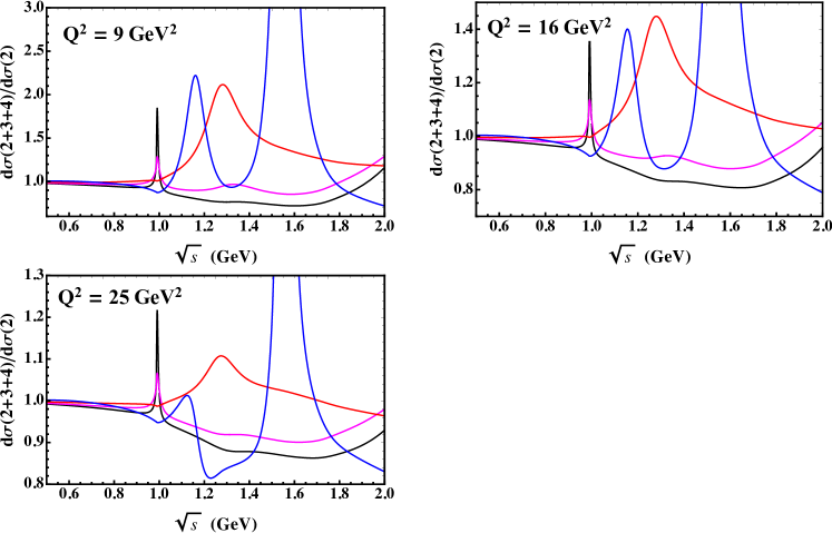
Figure 2: Ratio of $d\sigma_{t2+t3+t4}/d\sigma_{t2}$ with the pion GDA extracted from Belle measurements.

To sum-up this phenomenological study, let us stress that the uncertainties of Belle measurements Belle:2015oin are quite large, and the statistical errors are dominant. However, this situation will be improved substantially soon, since Belle II collaboration just started taking data at the SuperKEKB with a much higher luminosity. Precise measurements of $\gamma^{*}+\gamma\rightarrow M_{1}+M_{2}$ are expected in the near future, and an accurate description of the amplitudes will require the inclusion of kinematical contributions up to twist 4. This will be of utmost importance to address the question of the form factors of the pion energy-momentum tensor Kumano:2017lhr and of the impact-parameter picture representation of GDAs Pire:2002ut .

References

• (1) D.Β MΓΌller, D.Β Robaschik, B.Β Geyer, F.Β M.Β Dittes and J.Β HoΕ™ejΕ‘i, Fortsch. Phys. 42 (1994), 101-141.
• (2) M.Β Diehl, T.Β Gousset, B.Β Pire and O.Β Teryaev, Phys. Rev. Lett. 81 (1998), 1782-1785.
• (3) M.Β V.Β Polyakov, Nucl. Phys. B 555 (1999), 231.
• (4) M.Β Diehl, Phys. Rept. 388 (2003), 41-277.
• (5) V.Β M.Β Braun and A.Β N.Β Manashov, Phys. Rev. Lett. 107 (2011), 202001.
• (6) V.Β M.Β Braun and A.Β N.Β Manashov, JHEP 01 (2012), 085.
• (7) V.Β M.Β Braun and A.Β N.Β Manashov, Prog. Part. Nucl. Phys. 67 (2012), 162-167.
• (8) V.Β M.Β Braun, A.Β N.Β Manashov and B.Β Pirnay, Phys. Rev. D 86 (2012), 014003.
• (9) M.Β Diehl, T.Β Gousset and B.Β Pire, Phys. Rev. D 62 (2000), 073014.
• (10) M.Β Masuda et al. [Belle], Phys. Rev. D 93 (2016), 032003.
• (11) S.Β Kumano, Q.Β T.Β Song and O.Β V.Β Teryaev, Phys. Rev. D 97 (2018) no.1, 014020.
• (12) O.Β Nachtmann, Nucl. Phys. B 63 (1973), 237-247.
• (13) O.Β V.Β Teryaev, Phys. Lett. B 510 (2001), 125-132.
• (14) B.Β Pire and L.Β Szymanowski, Phys. Lett. B 556 (2003), 129-134.