Real-Time Distributed Model Predictive Control with Limited Communication Data Rates

Abstract

The application of distributed model predictive controllers (DMPC) for multi-agent systems (MASs) necessitates communication between agents, yet the consequence of communication data rates is typically overlooked. This work focuses on developing stability-guaranteed control methods for MASs with limited data rates. Initially, a distributed optimization algorithm with dynamic quantization is considered for solving the DMPC problem. Due to the limited data rate, the optimization process suffers from inexact iterations caused by quantization noise and premature termination, leading to sub-optimal solutions. In response, we propose a novel real-time DMPC framework with a quantization refinement scheme that updates the quantization parameters on-line so that both the quantization noise and the optimization sub-optimality decrease asymptotically. To facilitate the stability analysis, we treat the sub-optimally controlled MAS, the quantization refinement scheme, and the optimization process as three interconnected subsystems. The cyclic-small-gain theorem is used to derive sufficient conditions on the quantization parameters for guaranteeing the stability of the system under a limited data rate. Finally, the proposed algorithm and theoretical findings are demonstrated in a multi-AUV formation control example.

I Introduction

Model predictive control can systematically handle constraints in determining the control action. In multi-agent systems (MASs) without central decision-makers, distributed model predictive control (DMPC) offers a viable solution. To apply DMPC, the agents rely on communication networks for solving the underlying distributed optimization problems at every time step. Thus, it is necessary to consider the communication challenges ubiquitous in communication networks [1], e.g., communication delay, package loss, and limited communication data rate. In this paper, we focus on implementing DMPC for MASs with a limited data rate and aim to provide stability guarantees for the closed-loop system.

In [2], [3], distributed optimization algorithms that consider quantization noise arising from limited communication data rates are proposed and provide convergence guarantees when suitable quantization parameters are adopted. However, the fixed data rate not only causes inexact iterations but also limits the number of optimization iterations allowed, thus leading to sub-optimal solutions. In turn, the stability of the sub-optimally controlled system may not be guaranteed.

Sub-optimal MPC has been studied extensively, starting with [4]. In [5], [6], and [7], different MPC schemes are combined with real-time stability-guaranteeing mechanisms that are verified on-line. In [8] and [9], the small-gain theorem is used to derive sufficient conditions for the stability of dynamics-optimizer systems, where the former assumes Lipschitz continuity of the MPC problem and the latter considers MPC with only input constraints. In [10], the small-gain theorem is applied for stability analysis of a MAS interconnected with an output coordinator and nonlinear controllers. The works [11] and [12] involve on-line stopping criteria that guarantee the stability of sub-optimal DMPC. Despite their efficacy in dealing with sub-optimality, these methods are not readily applicable in DMPC with limited communication data rates. There are DMPC schemes designed considering communication data rate. The work [13] compresses shared data with neural networks to save communication data rate and proves input-to-state-practical stability. In [14], a single-chain communication topology is considered and stability is guaranteed with a sufficiently long prediction horizon. While the above methods aim to reduce the communication data rate required for solving the DMPC problem, they do not explicitly consider the effect of the limited data rate on the closed-loop stability.

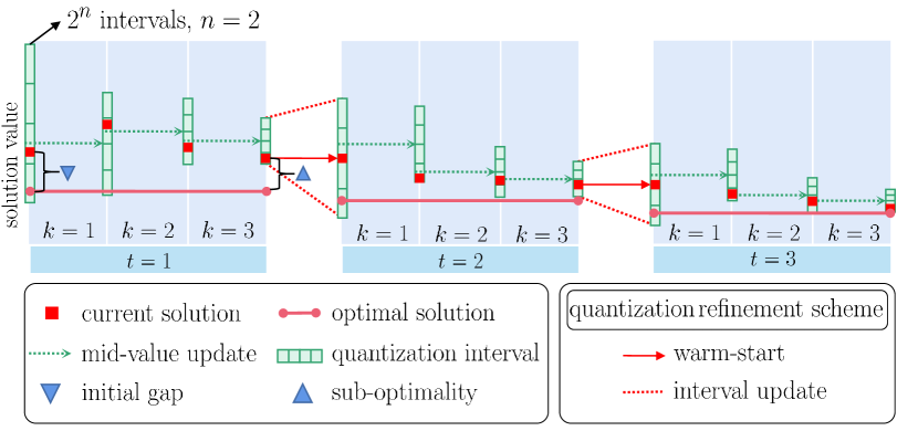
Figure 1: The on-line quantization refinement scheme.

In this work, we propose a DMPC framework for controlling a MAS under a limited data rate, with explicitly guaranteed closed-loop stability. Our previous work [15] is an initial step in this direction, which solves DMPC problems using the distributed optimization algorithm in [2] with quantization parameters determined off-line considering a limited data rate. Compared to [15], we refine the quantization parameters on-line to adapt to the change in sub-optimality and use a different stability analysis method, which allows for stronger stability guarantees. Specifically, we make the following main contributions:

• We propose a novel real-time DMPC framework with a quantization refinement scheme. The scheme includes an off-line stage that designs initial quantization parameters given a limited communication data rate, and an on-line stage (illustrated in Fig. 1) that implements the quantization refinement scheme, the optimization process, and the DMPC controller.

• Given a limited data rate, we derive sufficient, off-line-determined conditions on the quantization parameters such that the system controlled by the proposed framework is recursively feasible and stable. Specifically, we consider the sub-optimally controlled MAS, the quantization refinement scheme, and the optimization process as three interconnected subsystems. This formulation facilitates stability analysis of the closed-loop system using the cyclic-small-gain theorem, leading to input-to-state stability (ISS) guarantee w.r.t a quantization refinement parameter that associates with state estimation error.

II Preliminaries

For an optimization problem and an optimization algorithm, let $z^{*}$ and $z^{k}\in\mathbb{R}^{m_{z}}$ denote the optimal and $k_{\text{th}}$-iteration solutions, respectively. Let the subscript $t$ denote the discrete time step of a controlled system. Let $I$ denote the identity matrix and Id denote the identity function. Let $\mathbb{S}^{n}_{++}$ denote the set of all positive definite matrices with size $n\times n$. For a vector $x\in\mathbb{R}^{m_{x}}$ and a matrix $H\in\mathbb{S}^{m_{x}}_{++}$, let $\|x\|_{\infty}$, $\|x\|$, and $\|x\|_{H}$ denote the $\infty$-norm, $2$-norm, and the weighted 2-norm of $x$, respectively. Note that $\|x\|_{\infty}\leq\|x\|\leq\sqrt{m_{x}}\|x\|_{\infty}$. Let $\|H\|$ denote the induced norm of $H$. Let $\underline{\lambda}(H)$ and $\overline{\lambda}(H)$ denote the smallest and largest eigenvalues of $H$, respectively. For a continuous function $\alpha(s)$, $\alpha(s)\in\mathcal{K}$ if $\alpha(0)=0$ and $\dot{\alpha}(s)>0$. Furthermore, $\alpha(s)\in\mathcal{K}_{\infty}$ if $\alpha(s)$ is unbounded. Given functions $\alpha_{1}(w):\mathcal{W}\rightarrow\mathcal{Y}$ and $\alpha_{2}(y):\mathcal{Y}\rightarrow\mathcal{Z}$, we define $\alpha_{1}\circ\alpha_{2}(w)=\alpha_{2}(\alpha_{1}(w)):\mathcal{W}\rightarrow\mathcal{Z}$. The operators $\left\lceil\cdot\right\rceil$ and $\left\lfloor\cdot\right\rfloor$ denote the ceil and floor operations, respectively. The operator $\operatorname{blkdiag}(H_{1},\cdots,H_{m})$ yields a matrix $H$ containing the matrices $H_{1},\cdots,H_{m}$ in its diagonal. We denote the projection of a vector $z\in\mathbb{R}^{m_{z}}$ onto the set $\mathcal{C}\subseteq\mathbb{R}^{m_{z}}$ as $\operatorname{Proj}_{\mathcal{C}}(z):=\operatorname{argmin}_{\bar{z}\in\mathcal{C}}\|\bar{z}-z\|$. Let the uniform quantizer be defined as $Q(x):=\bar{x}+\operatorname{sgn}(x-\bar{x})\cdot\frac{l}{2^{n}}\cdot\left\lfloor\frac{\|x-\bar{x}\|}{{l}/{2^{n}}}+\frac{1}{2}\right\rfloor$, with mid-value $\bar{x}$, quantization interval $l$, and bit number $n$. The cyclic-small-gain theorem presented below is relevant to the stability analysis:

Lemma 1 (Lemma 1, [16]).

Consider an interconnected system composed of $M$ subsystems with discrete dynamics

$$x_{i,t+1}=f_{i}(x_{i,t},x_{j,t},u_{i,t}),\;\forall i,j\in\{1,\cdots,M\},i\neq j,$$ (1)

where $x_{i,t}$, $x_{j,t}$, and $u_{i,t}$ denote the states, interconnected states, and external inputs, respectively. Suppose each subsystem admits a continuous ISS-Lyapunov function satisfying

$$\tilde{\alpha}_{i,l}\left(\|x_{i,t}\|\right) \leq V_{i}\left(x_{i,t}\right)\leq\tilde{\alpha}_{i,u}\left(\|x_{i,t}\|\right),$$ (2)

$$V_{i}(x_{i,t+1}) -V_{i}(x_{i,t})\leq-\tilde{\alpha}_{i}(V_{i}(x_{i,t}))$$

$$+\max_{j\in\{1,\cdots,M\},j\neq i}\left(\tilde{\gamma}_{i,j}(V_{j}(x_{j,t})),\tilde{\gamma}_{i}^{e}(\|x^{e}_{i,t}\|)\right),$$ (3)

where $\tilde{\alpha}_{i,l},\tilde{\alpha}_{i,u},\tilde{\alpha}_{i}\in\mathcal{K}_{\infty}$, $\left(\mathrm{Id}-\tilde{\alpha}_{i}\right)\in\mathcal{K}$ and $\tilde{\gamma}_{i,j},\tilde{\gamma}_{i}^{e}\in\mathcal{K}\cup\{0\}$. Then, the interconnected system is ISS with $u_{t}=[u_{1,t}^{\top},\allowbreak\cdots,\allowbreak u_{M,t}^{\top}]^{\top}$ as the input, if there exist positive definite functions $\tilde{\mu}_{i}$ satisfying $\mathrm{Id}-\tilde{\mu}_{i}\in\mathcal{K}_{\infty}$ such that the ISS gain functions $\mathcal{X}_{i,j}:=\tilde{\alpha}_{i}^{-1}\circ\left(\mathrm{Id}-\tilde{\mu}_{i}\right)^{-1}\circ\tilde{\gamma}_{i,j}$ satisfy

$$\mathcal{X}_{j,j^{\prime}}\circ\mathcal{X}_{j^{\prime},j^{\prime\prime}}\circ\cdots\circ\mathcal{X}_{r,j}<\textup{ Id }$$ (4)

for each $r=\{2,\cdots,M\}$ and all $1\leq j<j^{\prime}<j^{\prime\prime}<r$, i.e., for all the interconnected cycles in the system.

III Distributed Optimization with Quantization

We solve a class of DMPC problems over a system of $M$ agents that communicate synchronously under limited communication data rates via an undirected graph $\mathcal{G}=(\mathcal{M},\mathcal{E})$, with vertex set $\mathcal{M}=\{1,\cdots,M\}$ and edge set $\mathcal{E}\subseteq\mathcal{M}\times\mathcal{M}$. If $(i,j)\in\mathcal{E}$, then agent $i$ and $j$ are neighbours and communicate with each other. Let $\mathcal{N}_{i}=\{j\mid(i,j)\in\mathcal{E}\}$ denote the set of neighbors of agent $i$, including agent $i$ itself. Let $d$ denote the degree of $\mathcal{G}$. The DMPC problems can be formulated as the following distributed optimization problem:

$$\min_{z}\; f\left(z\right)=\sum_{i\in\mathcal{M}}f_{i}\left(z_{\mathcal{N}_{i}}\right),$$ (5)

s.t. $$z_{i}\in\mathcal{C}_{i},z_{\mathcal{N}_{i}}=\;E_{i}z,z_{j}=F_{ij}z_{\mathcal{N}_{i}},$$

where $z=[z_{1}^{\top},\cdots,z_{M}^{\top}]^{\top}\in\mathbb{R}^{m_{z}}$ and $z_{i}\in\mathbb{R}^{m_{z_{i}}}$ denote the global and local decision variables, respectively. Let $E_{i}\in\mathbb{R}^{m_{z_{i}}\times m_{z}}$, $F_{ji}\in\mathbb{R}^{{m_{z_{\mathcal{N}_{i}}}}\times m_{z}}$ be the selection matrices defined w.r.t. $\mathcal{N}_{i}$. Let $z_{\mathcal{N}_{i}}$ be the stacked decision variables of the agents in ${\mathcal{N}_{i}}$. Let $\bar{m}:=\max_{i\in\mathcal{M}}m_{z_{i}}$ denote the largest size of local decision variables. Let $\mathcal{C}_{i}$ be the local constraint set.

Assumption 1.

All the local constraint sets $\mathcal{C}_{i}$ are convex.

Assumption 2.

All local cost functions $f_{i}(\cdot)$ are strongly convex with Lipschitz continuous gradients $\nabla f_{i}(\cdot)$ satisfying $\|\nabla f_{i}(z_{i,t_{1}})-\nabla f_{i}(z_{i,{t_{2}}})\|\leq L_{i}\|z_{i,t_{1}}-z_{i,t_{2}}\|$ for any $z_{i,t_{1}}$ and $z_{i,t_{2}}$.

Assumption 2 implies the global cost function $f(\cdot)$ is strongly convex with a convexity modulus $\alpha_{f}$ and a Lipschitz continuous gradient $\nabla f(\cdot)$ satisfying $\|\nabla f(z_{t_{1}})-\nabla f(z_{t_{2}})\|\leq L_{f}\|z_{t_{1}}-z_{t_{2}}\|$.

Algorithm 1 Distributed Optimization with Dynamic Quantization

Require: Initialize $\check{z}^{-1}_{i}=z^{0}_{i}$ $\check{\nabla}f^{-1}_{i}=\nabla f_{i}(\operatorname{Proj}_{\mathcal{C}_{\mathcal{N}_{i}}}(z_{\mathcal{N}_{i}}^{0}))$, $C_{i}$, $K$, $(1-\gamma)<\rho<1$, $\gamma=\frac{\alpha_{f}}{L_{f}}$, and $\eta<\frac{1}{L_{f}}$;

for $k=0,1,\cdots,K$ do

     for $\text{agent }i\in\mathcal{M}$ do $\triangleright$ in parallel

         1. Update $l_{i}^{k}=\rho^{k}C_{i}$ and $\bar{z}_{i}^{k}=\check{z}_{i}^{k-1}$ for $Q_{\alpha,i}^{k}$;

         2. Quantize local variable: $\check{z}_{i}^{k}=Q_{\alpha,i}^{k}\left(z_{i}^{k}\right)$;

         3. Send $\check{z}^{k}_{i}$ to agent $j$ for all $j\in\mathcal{N}_{i}$;

         4. Compute the projection: $\tilde{z}_{\mathcal{N}_{i}}^{k}=\operatorname{Proj}_{\mathcal{C}_{\mathcal{N}_{i}}}\left(\check{z}_{\mathcal{N}_{i}}^{k}\right)$;

         5. Compute $\nabla f^{k}_{i}=\nabla f_{i}\left(\tilde{z}_{\mathcal{N}_{i}}^{k}\right)$;

         6. Update $l_{i}^{k}=\rho^{k}C_{i}$ and $\bar{\nabla}f_{i}^{k}=\check{\nabla}f_{i}^{k-1}$ for $Q_{\beta,i}^{k}$;

         7. Quantize local gradient: $\check{\nabla}f_{i}^{k}=Q_{\beta,i}^{k}\left(\nabla f_{i}^{k}\right)$;

         8. Send $\check{\nabla}f^{k}_{i}$ to agent $j$ for all $j\in\mathcal{N}_{i}$;

         9. $z^{k+1}_{i}=\mathrm{Proj}_{\mathcal{C}_{i}}\left(z^{k}_{i}-\eta\sum_{j\in\mathcal{N}_{i}}F_{ji}\check{\nabla}f_{j}^{k}\right)$;

     end for

end for

To solve (5), we consider Alg. 1, modified from the distributed optimization algorithm with dynamic quantization proposed in [2]. Uniform quantizers $Q_{\alpha,i}^{k}$ and $Q_{\beta,i}^{k}$ are used by agent $i$ for transmitting local decision variables $z^{k}_{i}$ and gradients $\nabla f^{k}_{i}$ at iteration $k$, respectively. They are parametrized by the quantization bit number $n$, quantization interval $l^{k}_{i}$, and mid-values $\bar{z}_{i}^{K}$ and $\bar{\nabla}f_{i}^{k}$, respectively. The quantization interval is progressively updated according to $l^{k}_{i}=C_{i}\rho^{k}$, with base quantization interval $C_{i}$ and the shrinkage constant $\rho\in(1-\gamma,1)$, $\gamma={\alpha_{f}}/{L_{f}}\in(0,1)$. The mid-values are updated according to $\bar{z}_{i}^{k}=\check{z}_{i}^{k-1}$ and $\bar{\nabla}f_{i}^{k}=\check{\nabla}f_{i}^{k-1}$. The projections $\operatorname{Proj}_{\mathcal{C}_{\mathcal{N}_{i}}}$ and $\operatorname{Proj}_{\mathcal{C}_{i}}$ ensure the quantized variable $\check{z}_{\mathcal{N}_{i}}^{k}$ and the local solution computed from quantized gradient $\check{\nabla}f_{j}^{k}$ are feasible despite the quantization noises, for all iteration $k\geq 0$. The constraint set $\mathcal{C}_{\mathcal{N}_{i}}=\mathcal{C}_{i}\times\cdots\times\mathcal{C}_{j}$ represents the constraints of all the agents in $\mathcal{N}_{i}$. Let $\eta$ denote the optimization step-size. Each blue block in Fig. 1 corresponds to the implementation of Alg. 1 for $n=2$ and $K=3$.

The main difference between Alg. 1 and [2] is we initialize the local quantizers $Q_{\alpha,i}^{k}$ and $Q_{\beta,i}^{k}$ of agent $i$ with a local base quantization interval $C_{i}$ instead of a global one. This change eases the need for the agents to agree on a base quantization interval through centralized communication. Correspondingly, we propose a new condition on the base quantization interval $C_{i}$ and the bit number $n$, and a new convergence bound for Alg. 1.

Lemma 2.

Consider Alg. 1 applied to solve problem (5). Suppose Assumptions 1 and 2 hold. Let $z^{0}$ be the initial solution and ${\Delta z^{0}}:=z^{0}-z^{*}$ be the initial gap. If the quantization bit number $n$ satisfies

$$2^{n}\rho-\sqrt{d\bar{m}}>0,$$ (6)

and the local base quantization interval $C_{i}$ satisfies

$$a_{1}\|{\Delta z^{0}}\|+a_{2}C_{\Sigma}\leq C_{i},\;i\in\mathcal{M},$$ (7)

then the sub-optimality ${\Delta z^{K}}:=z^{K}-z^{*}$ generated by Alg. 1 satisfies

$$\|{\Delta z^{K}}\|\leq\rho^{K}(\|{\Delta z^{0}}\|+a_{3}C_{\Sigma}),$$ (8)

where $C_{\Sigma}:=\sum_{i\in\mathcal{M}}C_{i}$ and

$$a_{1}:= \max(\frac{2^{n+1}\max_{i\in\mathcal{M}}(L_{i})(1+\rho)}{2^{n}\rho-\sqrt{d\bar{m}}},{2(1+\rho)}/{\rho}),\allowdisplaybreaks$$ (9)

$$a_{2}:= \max(\frac{\max_{i\in\mathcal{M}}(L_{i})(1+\rho)(2^{n+1}a_{3}+{\sqrt{\bar{m}}})}{2^{n}\rho-\sqrt{d\bar{m}}},\allowdisplaybreaks$$

$$\qquad\;\;\;({2^{n+1}(1+\rho)a_{3}+\sqrt{\bar{m}}})/({2^{n}\rho})),\allowdisplaybreaks$$

$$a_{3}:= \frac{\sqrt{\bar{m}}(M\max_{i\in\mathcal{M}}(L_{i})+\sqrt{L_{f}d}+\sqrt{d})\rho}{L_{f}(\rho+\gamma-1)(1-\gamma)2^{n+1}}.$$

Proof.

The proof contains two parts: (i) inspired by Lemma 3.10 [2], we develop a one-step bound on $\|{\Delta z^{p+1}}\|$ in the form of (8) which holds if the quantization errors are bounded at iteration $p$. (ii) inspired by Lemma 3.17 [2], we use induction to show the quantization errors are bounded at every iteration $k$ and the one-step convergence bound holds at every iteration $k$.

(i) We first construct the one-step bound. For a uniform quanitzer $Q(z)$ with quantization interval $l$ and bit number $n$, if the input $z$ falls inside the quantization interval of $Q(z)$, then it holds that

$$\|z-Q(z)\|\leq\frac{l}{2^{n+1}}.$$ (10)

When $k=p$, if $z_{i}^{p}$ and $\nabla f_{i}^{p}$ fall inside the quantization intervals of $Q_{\alpha,i}^{p}$ and $Q_{\beta,i}^{p}$, respectively, then the quantization errors $\alpha_{i}^{p}=\check{z}_{i}^{p}-z_{i}^{p}$ and $\beta_{i}^{p}=\check{\nabla}f_{i}^{p}-\nabla f_{i}^{p}$ satisfy

$$\left\|\alpha_{i}^{p}\right\| \leq\sqrt{m_{i}}\left\|\alpha_{i}^{p}\right\|_{\infty}\overset{\eqref{quant error bound}}{\leq}\sqrt{\bar{m}}\frac{l_{i}^{p}}{2^{n+1}}=\sqrt{\bar{m}}\frac{\rho^{p}C_{i}}{2^{n+1}},$$ (11)

$$\left\|\beta_{i}^{p}\right\| \leq\sqrt{\sum_{j\in\mathcal{N}_{i}}m_{i}}\left\|\beta_{i}^{p}\right\|_{\infty}\overset{\eqref{quant error bound}}{\leq}\sqrt{d\bar{m}}\frac{l_{i}^{p}}{2^{n+1}}=\sqrt{d\bar{m}}\frac{\rho^{p}C_{i}}{2^{n+1}},$$ (12)

respectively. From Lemma 3.8 [2], the error sequences from Alg. 1,

$$\mathrm{e}^{p}=\sum_{i\in\mathcal{M}}E_{i}^{T}\nabla f_{i}\left(\tilde{z}_{\mathcal{N}_{i}}^{p}\right)+\sum_{i\in\mathcal{M}}E_{i}^{T}\beta_{i}^{p}-\sum_{i\in\mathcal{M}}E_{i}^{T}\nabla f_{i}\left({\mathcal{N}_{i}}^{p}\right)$$

and $\epsilon^{p}=\frac{1}{2}\|z^{p}-\tilde{z}^{p}\|^{2}$ satisfy

$$\|\mathrm{e}^{p}\|\leq \sum_{i\in\mathcal{M}}L_{i}\sum_{j\in\mathcal{N}_{i}}\|\alpha_{j}^{p}\|+\sum_{i\in\mathcal{M}}\|\beta_{i}^{p}\|$$ (13)

$$\sqrt{\epsilon^{p}}\leq \frac{\sqrt{2}}{2}\sum_{i\in\mathcal{M}}\|\alpha_{i}^{p}\|,$$ (14)

respectively. Then, applying the bounds in (11) and (12) to (13) and (14), we obtain

$$\left\|\mathrm{e}^{p}\right\| \leq\frac{\sqrt{\bar{m}}}{2^{n+1}}(\max_{i\in\mathcal{M}}(L_{i})\sum_{i\in\mathcal{M}}\sum_{j\in\mathcal{N}_{i}}C_{j}+\sqrt{d}C_{\Sigma})\rho^{p}\leq C_{a}\rho^{p},$$ (15)

$$\sqrt{\epsilon^{p}} \leq\frac{\rho^{p}\sqrt{2d\bar{m}}}{2^{n+2}}C_{\Sigma}=C_{b}\rho^{p},$$ (16)

where $C_{a}=\frac{\sqrt{\bar{m}}}{2^{n+1}}(\max_{i\in\mathcal{M}}(L_{i})MC_{\Sigma}+\sqrt{d}C_{\Sigma})$ and $C_{b}=\frac{\sqrt{2d\bar{m}}}{2^{n+2}}C_{\Sigma}$. In Proposition 2.5 of [2], it is proven that

$$\|z^{p+1}-z^{*}\|\leq(1-\gamma)^{p+1}(\|z^{0}-z^{*}\|+\Gamma^{p}),$$ (17)

where

$$\Gamma^{p}=\sum_{p=0}^{p}(1-\gamma)^{-q-1}\left(\frac{1}{L_{f}}\|\mathrm{e}^{q}\|+\sqrt{\frac{2}{L_{f}}}\sqrt{\epsilon^{q}}\right)$$ (18)

accounts for the inexactness in an iteration of the inexact proximal-gradient method. Plugging (18) into the r.h.s of (17), using (15) and (16) to bound $\left\|e^{p}\right\|$ and $\sqrt{\epsilon^{p}}$, respectively, and using the fact that $0<(1-\gamma)<\rho<1$, we obtain

$$\|\Delta z^{p+1}\|=\|z^{p+1}-z^{*}\|$$

$$\leq (1-\gamma)^{p+1}\|\Delta z^{0}\|$$ (19)

$$+\frac{\left(C_{a}+\sqrt{2L_{f}}C_{b}\right)}{L_{f}}\sum_{q=0}^{p}\rho^{q}(1-\gamma)^{p+1-q-1}$$ (20)

$$\leq \rho^{p+1}\left(\|\Delta z^{0}\|+\frac{(C_{a}+\sqrt{2L_{f}}C_{b})}{L_{f}(1-\gamma)}\sum_{q=0}^{p}\left((1-\gamma)/\rho\right)^{p+1-q}\right)$$ (21)

$$\leq \rho^{p+1}\left(\|\Delta z^{0}\|+\frac{(C_{a}+\sqrt{2L_{f}}C_{b})}{L_{f}(1-\gamma)}\frac{1-\left((1-\gamma)/\rho\right)^{p+1}}{1-(1-\gamma)/\rho}\right)$$ (22)

$$\leq \rho^{p+1}\left(\|\Delta z^{0}\|+\frac{(C_{a}+\sqrt{2L_{f}}C_{b})\rho}{L_{f}(1-\gamma)(\rho+\gamma-1)}\right)$$ (23)

$$= \rho^{p+1}(\|\Delta z^{0}\|+a_{3}C_{\Sigma}),$$ (24)

where the property of geometric series is used to obtain (22) by bounding $\sum_{q=0}^{p}\left((1-\gamma)/\rho\right)^{p+1-q}$ in (21). The term $a_{3}$ in (24), which is defined in (9), is obtained by plugging $C_{a}$ and $C_{b}$ into (23) and carrying out simplification.

(ii) We prove by induction that $z_{i}^{k}$ and $\nabla f_{i}^{k}$ fall inside the quantization intervals of $Q_{\alpha,i}^{k}$ and $Q_{\beta,i}^{k}$, respectively, for all $k\geq 0$, so that the one-step bound in (23) holds at every step.

Base case: When $k=0$, we initialize $C_{i}>0$ and $\check{z}_{i}^{-1}=z_{i}^{0}=0$ $\forall i\in\mathcal{M}$, which satisfies

$$\|z_{i}^{0}-\bar{z}_{i}^{0}\|_{\infty}=\|z_{i}^{0}-\check{z}_{i}^{-1}\|_{\infty}=0\leq\frac{l_{i}^{0}}{2}=\frac{C_{i}}{2},$$ (25)

$$\|\nabla f_{i}^{0}-\bar{\nabla}f_{i}^{0}\|_{\infty}=\|\nabla f_{i}^{0}-\check{\nabla}f_{i}^{-1}\|_{\infty}$$

$$=\|\nabla f_{i}(\tilde{z}_{\mathcal{N}_{i}}^{0})-\nabla f_{i}(\operatorname{Proj}_{\mathcal{C}_{\mathcal{N}_{i}}}(0))\|=0\leq\frac{l_{i}^{0}}{2}=\frac{C_{i}}{2}.$$ (26)

Thus, bounded quantization errors imply the input variable are bounded by the quantization intervals of the quantizers.

Induction case: When $k=p\geq 0$, suppose $\|z_{i}^{k}-\bar{z}_{i}^{k}\|_{\infty}\leq{l_{i}^{k}}/{2}$ and $\|\nabla f_{g}^{k}-\bar{\nabla}f_{i}^{k}\|_{\infty}\leq{l_{i}^{k}}/{2}$ for $0\leq k\leq p$. We need to prove

$$\|z_{i}^{p+1}-\bar{z}_{i}^{p+1}\|_{\infty}\leq{l_{i}^{p+1}}/{2},$$ (27)

$$\|\nabla f_{g}^{p+1}-\bar{\nabla}f_{i}^{p+1}\|_{\infty}\leq{l_{i}^{p+1}}/{2}.$$ (28)

We first prove (27). The quantization error from Alg. 1 satisfies

$$\|z_{i}^{p+1}-\bar{z}_{i}^{p+1}\|_{\infty}=\|z_{i}^{p+1}-\check{z}_{i}^{p}\|_{\infty}\leq\|z^{p+1}-\check{z}^{p}\|_{\infty}\allowdisplaybreaks$$ (29)

$$= \|z^{p+1}-z^{p}-\sum_{i\in\mathcal{M}}E_{i}^{T}F_{ii}^{T}\alpha_{i}^{p}\|_{\infty}\allowdisplaybreaks$$ (30)

$$\leq \|z^{p+1}-z^{p}\|_{\infty}+\|\sum_{i\in\mathcal{M}}E_{i}^{T}F_{ii}^{T}\alpha_{i}^{p}\|_{\infty}\allowdisplaybreaks$$ (31)

$$\leq \|z^{p+1}-z^{\star}\|_{\infty}+\|z^{p}-z^{\star}\|_{\infty}+\|\sum_{i\in\mathcal{M}}E_{i}^{T}F_{ii}^{T}\alpha_{i}^{p}\|_{\infty}\allowdisplaybreaks$$ (32)

$$\leq \|\Delta z^{p+1}\|+\|\Delta z^{p}\|+\sum_{i\in\mathcal{M}}\|\alpha_{i}^{p}\|,$$ (33)

where we used $\|E_{i}\|=\|F_{ij}\|=1$ to obtain (33). Since $\|z_{i}^{k}-\bar{z}_{i}^{k}\|_{\infty}\leq{l_{i}^{k}}/{2}$ and $\|\nabla f_{g}^{k}-\bar{\nabla}f_{i}^{k}p\|_{\infty}\leq{l_{i}^{k}}/{2}$ for $k=p$ and $k=p-1$, we can bound $\|\Delta z^{p+1}\|$ and $\|\Delta z^{p}\|$ with (24) and use (11) to obtain

$$\|z_{i}^{p+1}-\bar{z}_{i}^{p+1}\|_{\infty}$$

$$\leq \rho^{p+1}(\|\Delta z^{0}\|+a_{3}C_{\Sigma})+\rho^{p}(\|\Delta z^{0}\|+a_{3}C_{\Sigma})$$

$$+\rho^{p}\frac{\sqrt{\bar{m}}}{2^{n+1}}C_{\Sigma},$$ (34)

$$\leq \frac{\rho^{p+1}}{2}(a_{1}\|\Delta z^{0}\|+a_{2}C_{\Sigma})$$ (35)

where (35) holds from the definitions of $a_{1}$, $a_{2}$ in (9), and the condition (6). Then, condition (7) implies (27) holds for all $k=p\geq 0$.

We then prove (28). From Alg. 1, the gradient satisfies

$$\|\nabla f_{i}^{p+1}-\bar{\nabla}f_{i}^{p+1}\|_{\infty}=\|\nabla f_{i}^{p+1}-\check{\nabla}f_{i}^{p}\|_{\infty}$$ (36)

$$= \|\nabla f_{i}\left(\tilde{z}_{\mathcal{N}_{i}}^{p+1}\right)-\nabla f_{i}\left(\tilde{z}_{\mathcal{N}_{i}}^{p}\right)+\beta_{i}^{p}\|_{\infty}$$ (37)

$$\leq \|\nabla f_{i}\left(\tilde{z}_{\mathcal{N}_{i}}^{p+1}\right)-\nabla f_{i}\left(\tilde{z}_{\mathcal{N}_{i}}^{p}\right)\|+\|\beta_{i}^{p}\|$$ (38)

$$\leq L_{i}\|\tilde{z}_{\mathcal{N}_{i}}^{p+1}-\tilde{z}_{\mathcal{N}_{i}}^{p}\|+\|\beta_{i}^{p}\|$$ (39)

$$\leq L_{i}(\|z_{\mathcal{N}_{i}}^{p+1}-z_{\mathcal{N}_{i}}^{p}\|+\|\tilde{z}_{\mathcal{N}_{i}}^{p+1}-z_{\mathcal{N}_{i}}^{p+1}\|+\|\tilde{z}_{\mathcal{N}_{i}}^{p}-z_{\mathcal{N}_{i}}^{p}\|)+\|\beta_{i}^{p}\|.$$ (40)

Since $\check{z}_{\mathcal{N}_{i}}^{p},\check{z}_{\mathcal{N}_{i}}^{p+1}\in\mathcal{C}_{\mathcal{N}_{i}}$, we have from Lemma 3.7 [2] that

$$\|\tilde{z}_{\mathcal{N}_{i}}^{p}-z_{\mathcal{N}_{i}}^{p}\|=\|\operatorname{Proj}_{\mathcal{C}_{\mathcal{N}_{i}}}(\check{z}_{\mathcal{N}_{i}}^{p})-z_{\mathcal{N}_{i}}^{p}\|\leq\|\check{z}_{\mathcal{N}_{i}}^{p}-z_{\mathcal{N}_{i}}^{p}\|,$$ (41)

$$\|\tilde{z}_{\mathcal{N}_{i}}^{p+1}-z_{\mathcal{N}_{i}}^{p+1}\|=\|\operatorname{Proj}_{\mathcal{C}_{\mathcal{N}_{i}}}(\check{z}_{\mathcal{N}_{i}}^{p+1})-z_{\mathcal{N}_{i}}^{p+1}\|\leq\|\check{z}_{\mathcal{N}_{i}}^{p+1}-z_{\mathcal{N}_{i}}^{p+1}\|.$$ (42)

Applying the above bounds to (40), we obtain

$$\|\nabla f_{i}^{p+1}-\bar{\nabla}f_{i}^{p+1}\|_{\infty}$$

$$\leq L_{i}(\|z_{\mathcal{N}_{i}}^{p+1}-z_{\mathcal{N}_{i}}^{p}\|+\|\check{z}_{\mathcal{N}_{i}}^{p+1}-z_{\mathcal{N}_{i}}^{p+1}\|+\|\check{z}_{\mathcal{N}_{i}}^{p}-z_{\mathcal{N}_{i}}^{p}\|)+\|\beta_{i}^{p}\|$$ (43)

$$\leq L_{i}\|z_{\mathcal{N}_{i}}^{p+1}-z_{\mathcal{N}_{i}}^{p}\|+L_{i}\sum_{j\in\mathcal{N}_{i}}(\|\alpha_{j}^{p+1}\|+\|\alpha_{j}^{p}\|)+\|\beta_{i}^{p}\|$$ (44)

$$\leq L_{i}\|z^{p+1}-z^{p}\|+L_{i}\sum_{j\in\mathcal{N}_{i}}(\|\alpha_{j}^{p+1}\|+\|\alpha_{j}^{p}\|)+\|\beta_{i}^{p}\|$$ (45)

$$\leq\max_{i\in\mathcal{M}}(L_{i})(\|\Delta z^{p+1}\|+\|\Delta z^{p}\|$$

$$\quad+\sum_{j\in\mathcal{N}_{i}}(\|\alpha_{j}^{p+1}\|+\|\alpha_{j}^{p}\|))+\|\beta_{i}^{p}\|.$$ (46)

Due to the induction assumption, we can bound $\|\Delta z^{p+1}\|$ and $\|\Delta z^{p}\|$ in (46) with (24), and then use (11) and (12), to obtain

$$\|\nabla f_{i}^{p+1}-\bar{\nabla}f_{i}^{p+1}\|_{\infty}$$

$$\leq \max_{i\in\mathcal{M}}(L_{i})\rho^{p+1}(\|\Delta z^{0}\|+a_{2}C_{\Sigma})+\rho^{p}(\|\Delta z^{0}\|+a_{2}C_{\Sigma})$$

$$+\max_{i\in\mathcal{M}}(L_{i})\sum^{M}_{i=1}(\|\alpha_{i}^{p+1}\|+\|\alpha_{i}^{p}\|)+\|\beta_{i}^{p}\|$$ (47)

$$\leq \rho^{p}\max_{i\in\mathcal{M}}(L_{i})(1+\rho)(\|\Delta z^{0}\|+a_{2}C_{\Sigma})$$

$$+\frac{\rho^{p}\max_{i\in\mathcal{M}}(L_{i})\sqrt{\bar{m}}}{2^{n+1}}(1+\rho)C_{\Sigma}+\frac{\rho^{p}\sqrt{d\bar{m}}}{2^{n+1}}C_{i}$$ (48)

$$\leq \frac{\rho^{p+1}}{2}(a_{1}(n)\|\Delta z^{0}\|+a_{2}(n)C_{\Sigma})$$ (49)

where (49) holds from the definitions of $a_{1}$, $a_{2}$ in (9), and the condition (6). Then, condition (7) implies (28) holds for all $k=p\geq 0$.

Finally, we combine the base case and the induction case to conclude (26) and (27) hold for all $k\geq 0$, i.e., the values $z^{k}_{i}$ and $\nabla f^{k}_{i}$ generated by Alg. 1 always fall inside the quantization intervals of $Q_{\alpha,i}^{k}$ and $Q_{\beta,i}^{k}$, respectively. As a result, the solution $z^{k}$ generated by Alg. 1 satisfies (24) for all $k\geq 0$, i.e., (8) holds.

IV Real-Time DMPC Framework with Quantization Refinement

In this section, we propose a novel real-time DMPC framework with a quantization refinement scheme. We first introduce the DMPC problem we aim to solve under a limited communication data rate.

IV-A DMPC with Coupled Cost Functions

Consider a MAS with $M$ agents whose dynamics are

$$x_{i,t+1}=A_{i}x_{i,t}+B_{i}u_{i,t},\>\>\forall i\in\mathcal{M},$$ (50)

with states $x_{i,t}\in\mathbb{R}^{m_{x_{i}}}$, inputs $u_{i,t}\in\mathbb{R}^{m_{u_{i}}}$, and $(A_{i},B_{i})$ being controllable. Agent $i$ can communicate locally with neighbouring agents in $\mathcal{N}_{i}$. The global dynamics of the MAS is

$${{X}_{t+1}=A{X}_{t}+B{U}_{t},}$$ (51)

where $A=\operatorname{blkdiag}(A_{1},\cdots,A_{M})$, $B=\operatorname{blkdiag}(B_{1},\cdots,B_{M})$, $X_{t}=[x_{1,t}^{\top},\cdots,x_{M,t}^{\top}]^{\top}$, and $U_{t}=[u_{1,t}^{\top},\cdots,x_{M,t}^{\top}]^{\top}$. We stabilize (51) to the origin using the following DMPC formulation:

$$(\textbf{X}^{*}_{t},\textbf{U}^{*}_{t})=\underset{{\mathbf{x}_{i,t},\mathbf{u}_{i,t}}}{\operatorname{argmin}}\sum_{i=1}^{M}\left(\sum_{\tau=0}^{N-1}\|[\mathrm{x}^{\top}_{\mathcal{N}_{i},t}(\tau),\mathrm{u}^{\top}_{\mathcal{N}_{i},t}(\tau)]^{\top}\|_{H_{i}}\right)$$

$$\quad\quad\quad\quad\quad\quad\quad\quad\;\;\;\;+\|\mathrm{x}_{i,t}(N)\|_{P_{i}},\allowdisplaybreaks$$ (52a)

$$\text{s.t.}\;\mathrm{x}_{i,t}(0)=x_{i,t},\allowdisplaybreaks$$ (52b)

$$\quad\;\,\mathrm{x}_{i,t}(\tau+1)=A_{i}\mathrm{x}_{i,t}(\tau)+B_{i}\mathrm{u}_{i,t}(\tau),\allowdisplaybreaks$$ (52c)

$$\quad\;\,(\mathrm{x}_{i,t}(\tau),\mathrm{u}_{i,t}(\tau))\in\mathcal{C}_{x,i}\times\mathcal{C}_{u,i},\allowdisplaybreaks$$ (52d)

$$\quad\;\,\mathrm{x}_{i,t}(N)\in\mathcal{C}_{f,i},$$ (52e)

$$\quad\;\,\tau=0,\cdots,N-1,\;\forall i\in\mathcal{M}.$$

The local decision variables include the sequences $\textbf{x}_{i,t}=[\mathrm{x}_{i,t}^{\top}(0),\allowbreak\cdots,\allowbreak\mathrm{x}^{\top}_{i,t}(N)]^{\top}$ and $\mathbf{u}_{i,t}\allowbreak=\allowbreak[\mathrm{u}^{\top}_{i,t}(0),\allowbreak\cdots,\allowbreak\mathrm{u}^{\top}_{i,t}(N-1)]^{\top}$. Let $\mathrm{x}_{\mathcal{N}_{i},t}(\tau)\allowbreak=\allowbreak[\mathrm{x}^{\top}_{i,t}(\tau),\allowbreak\cdots,\allowbreak\mathrm{x}^{\top}_{j,t}(\tau)]^{\top}$ and $\mathrm{u}_{\mathcal{N}_{i},t}(\tau)\allowbreak=[\mathrm{u}^{\top}_{i,t}(\tau),\allowbreak\cdots,\allowbreak\mathrm{u}^{\top}_{j,t}(\tau)]^{\top}$ be the concatenated decision variables of the agents in $\mathcal{N}_{i}$ for $\tau=0,\cdots,N-1$. The global decision variables include the sequences $\textbf{X}_{t}=[\mathrm{X}^{\top}_{t}(0),\cdots,\mathrm{X}^{\top}_{t}(N)]^{\top}$ and $\mathbf{U}_{t}\allowbreak=\allowbreak[\mathrm{U}^{\top}_{t}(0),\allowbreak\cdots,\allowbreak\mathrm{U}^{\top}_{t}(N-1)]^{\top}$, where $\mathrm{X}_{t}(\tau)=[\mathrm{x}_{1,t}^{\top}(\tau),\cdots,\mathrm{x}_{M,t}^{\top}(\tau)]^{\top}$ for $\tau=0,\cdots,N$ and $\mathrm{U}_{t}(\tau)\allowbreak=\allowbreak[\mathrm{u}_{1,t}^{\top}(\tau),\allowbreak\cdots,\allowbreak\mathrm{u}_{M,t}^{\top}(\tau)]^{\top}$ for $\tau=0,\cdots,N-1$. Let $\textbf{X}^{*}_{t}$ and $\mathbf{U}^{*}_{t}$ be the optimal solution. Local terminal cost $\|\cdot\|_{P_{i}}$ and stage cost with coupling $\|\cdot\|_{H_{i}}$ are considered, with $H_{i},P_{i}\in\mathbb{S}_{++}$. The convex sets $\mathcal{C}_{x,i}$, $\mathcal{C}_{u,i}$, and $\mathcal{C}_{f,i}$ represent the local state, input, and terminal constraint sets, respectively. We define matrices $Q,R,P\in\mathbb{S}_{++}$, which satisfy $\operatorname{blkdiag}(Q,R)=\sum_{i\in\mathcal{M}}{E_{i}^{\top}H_{i}E_{i}}$ and $P=\operatorname{blkdiag}(\allowbreak P_{1},\allowbreak\cdots,\allowbreak P_{M})$.

Assumption 3.

Consider the MAS (51). Let $l(X,U)=\|X\|_{Q}+\|U\|_{R}$, $l_{f}(X)\allowbreak=\allowbreak\|X\|_{P}$, and $\mathcal{C}_{f}\allowbreak=\allowbreak\mathcal{C}_{f,i}\allowbreak\times\allowbreak\cdots\allowbreak\times\allowbreak\mathcal{C}_{f,M}$. There exist local stabilizing control laws $K_{f,i}x_{i}$ such that the MAS (51) under $\pi_{f}(X):=[(K_{f,i}x_{i})^{\top},\cdots,(K_{f,M}x_{M})^{\top}]^{\top}$ satisfies, $\forall X\in\mathcal{C}_{f}$:

$\bullet\;\;AX+B\pi_{f}(X)\in\mathcal{C}_{f}\textup{ and }\pi_{f}(X)\in\mathcal{C}_{u,i}\times\cdots\times\mathcal{C}_{u,M}$,

$\bullet\;\;l_{f}(AX+B\pi_{f}(X))-l_{f}(X)\leq-l(X,\pi_{f}(X))$.

The DMPC problem (52) can be formulated as (5), with local and global decision variables $z_{i,t}=[\textbf{x}^{\top}_{i,t},\mathbf{u}^{\top}_{i,t}]^{\top}$ and $z_{t}\allowbreak=\allowbreak[\textbf{X}^{\top}_{t},\allowbreak\mathbf{U}^{\top}_{t}]^{\top}$, respectively. The local and global cost functions are $f_{i}(z_{\mathcal{N}_{i},t})\allowbreak=\allowbreak\|\mathrm{x}_{i,t}(N)\|_{P_{i}}\allowbreak+\allowbreak\sum_{\tau=0}^{N-1}\|[\mathrm{x}^{\top}_{\mathcal{N}_{i},t}(\tau),\mathrm{u}^{\top}_{\mathcal{N}_{i},t}(\tau)]^{\top}\|_{H_{i}}$ and $f(z_{t})=\|z_{t}\|^{2}_{H}=\sum_{i\in\mathcal{M}}f_{i}(z_{\mathcal{N}_{i},t})$ , respectively, where $H=\operatorname{blkdiag}(I_{N-1}\otimes{\operatorname{blkdiag}(Q,R)},P)$, with $\otimes$ the Kronecker product. The local constraint set $\mathcal{C}_{i}\allowbreak=\allowbreak\mathcal{C}_{x,i}\allowbreak\times\allowbreak\mathcal{C}_{u,i}\allowbreak\times\allowbreak\cdots\times\mathcal{C}_{f,i}$ is convex and satisfies Assumption 1. Since $H_{i},P_{i}\in\mathbb{S}_{++}$, Assumption 2 is satisfied, with $L_{i}=2\max(\overline{\lambda}(H_{i}),\overline{\lambda}(P_{i}))$. Thus, (52) formulated as (5) can be solved using Alg. 1 with the convergence guarantee in (8). Let $z_{t}^{*}=[\textbf{X}^{*\top}_{t},\allowbreak\mathbf{U}^{*\top}_{t}]^{\top}$ and $z_{t}^{K}=[\textbf{X}^{K\top}_{t},\allowbreak\mathbf{U}^{K\top}_{t}]^{\top}$ be the optimal and $K_{\text{th}}$-iteration sub-optimal solutions, respectively. The corresponding optimal and sub-optimal control laws are

$$\quad\pi^{*}(X_{t}) :=\mathrm{U}^{*}_{t}(0)=[{\mathrm{u}^{*\top}_{i,t}}(0),\cdots,{\mathrm{u}^{*\top}_{M,t}}(0)]^{\top}=\Xi z^{*}_{t},$$ (53)

$$\pi^{K}(X_{t}) :=\mathrm{U}^{K}_{t}(0)=[{\mathrm{u}^{K\top}_{i,t}}(0),\cdots,{\mathrm{u}^{K\top}_{M,t}}(0)]^{\top}=\Xi z^{K}_{t},$$ (54)

respectively, where $\Xi\in\mathbb{R}^{{m_{u}}\times{m_{z}}}$ is a selection matrix. Let the optimal cost of (52) be $V(X_{t}):=f(z^{*}_{t})=\|z^{*}_{t}\|^{2}_{H}$ .

Assumption 4.

Consider the DMPC problem (52), there exists a Lipschitz constant $L$ such that for two feasible initial states $X_{t_{1}}$ and $X_{t_{2}}$, it holds that

$$\|z^{*}_{t_{1}}-z^{*}_{t_{2}}\|\leq L\|X_{t_{1}}-X_{t_{2}}\|,$$ (55)

where $z^{*}_{t_{1}}$ and $z^{*}_{t_{2}}$ are the optimal solutions of (52) with initial states $X_{t_{1}}$ and $X_{t_{2}}$, respectively.

Remark 1.

Since (52) is a convex optimization problem parametrized by $X_{t}$, $L$ always exists [17]. When all the constraints in (52) are polytopic, the Lipschitz constant $L$ exists and can be determined as the maximal gain of the explicit MPC solution of (52) in [18]. When the DMPC problem (52) only contains input constraints, the Lipschitz constant $L$ can be determined analytically [9]. For more general problem setups, sampling-based methods can be used to estimate $L$ with specified probability guarantee [lip_estimate].

IV-B DMPC Framework with Quantization Refinement

Let $T$ be the given communication data rate, defined as the number of bits available per time step for one agent to transmit to another agent. The communication constraint $nK\leq T$ exists and limits the number of iterations $K$ that Alg. 1 can be implemented and introduces quantization noise into Alg. 1. We assume sufficient computation resources are provided for carrying out all computations. To address the communication constraint, we propose a DMPC framework with a quantization refinement scheme in Alg. 2, which contains an off-line stage for quantization parameter design and an on-line stage for quantization refinement and control input computation.

In the off-line stage, we assume all agents have access to the global information. Given data rate $T$, the quantization bit number $n$ and iteration number $K$ satisfying the communication constraint $nK\leq T$ are determined (Step 1). Then, the the global state $X_{0}$ is measured for computing the optimal solution $z^{*}_{0}$ (Step 2). For initialization (Step 3), the warm-start solution $z^{K}_{0}$ is set to $z^{*}_{0}$ and the base quantization intervals $C_{i,t}$ are set to $0$.

Algorithm 2 DMPC Framework with Quantization Refinement

Require: $T$, $L$, $(1-\gamma)<\rho<1$, $\eta<\frac{1}{L_{f}}$, $\gamma=\frac{\alpha_{f}}{L_{f}}$, $t=0$;

Off-line Stage:

1. Determine $n$ and $K$ satisfying $nK\leq T$;

2. Measure $X_{0}$ and compute the optimal solution $z^{*}_{0}$ of (52);

3. Initialize $z^{K}_{0}=z^{*}_{0}$ and $C_{i,0}=0$, $i\in\mathcal{M}$.

On-line Stage:

if $t=0$ then

     4. Set $\hat{X}_{i,0}=X_{0},i\in\mathcal{M}$ and apply optimal control $\pi^{*}(X_{t})$;

else

     5. Obtain $\hat{X}_{i,t}$ and compute $\Delta\hat{X}_{i,t-1}:=\hat{X}_{t}-\hat{X}_{i,t-1}$,

        $i\in\mathcal{M}$;

     6. Update base quantization interval $C_{i,t}$ using (56), $i\in\mathcal{M}$;

     7. Update initial solution $z^{0}_{\mathcal{N}_{i},t}\leftarrow z^{K}_{\mathcal{N}_{i},t-1}$, $i\in\mathcal{M}$;

     8. Formulate DMPC problem (52) as a distributed optimiza

        -tion problem (5) with $x_{i,t}$ as the time-varying parameter

        and solve it using Alg. 1 over the MAS (51) for $K$

        iterations with inputs $n$, $\rho$, $\eta$, $z^{0}_{i,t}$, $C_{i,t}$, $i\in\mathcal{M}$;

     9. Apply sub-optimal control $\pi^{K}(X_{t})$;

end if

10. Increase time step $t=t+1$;

In the on-line stage, at every time step $t$, we require each agent $i$ to obtain a local estimate $\hat{X}_{i,t}$ of the global state $X_{t}$. The estimate $\hat{X}_{i,t}$ consists of accurate measurements $x_{i,t},i\in\mathcal{N}_{i}$ (also used as initial states for the DMPC problem (52)) and estimates $\hat{x}_{j,t},j\in\mathcal{M}\backslash\mathcal{N}_{i}$. Let $e_{i,t}:=\hat{X}_{i,t}-X_{t}$ be the combined estimation error. When $t=0$, the local estimates $\hat{X}_{i,0}$ are set as $X_{0}$ from Step 2 and the optimal control $\pi^{K}(X_{t})$ is applied to each agent. When $t>0$, the agents compute an estimated global state change $\Delta\hat{X}_{i,t-1}:=\hat{X}_{i,t}-\hat{X}_{i,t-1}$ (Step 5) and update the local base quantization intervals (Step 6) with

$$C_{i,t}=b_{1}C_{i,t-1}+b_{2}\|{\Delta}\hat{X}_{i,t-1}\|+(b_{3}+b_{4}b_{5})e,$$ (56)

where $e\geq 0$ is an upper-bound of $e_{i,t}$ for all $t>0$, and

$$b_{1}:=\frac{\rho^{K}(1+Ma_{1}a_{3}-Ma_{2})}{1-Ma_{2}},b_{2}:=\frac{La_{1}}{1-Ma_{2}},b_{5}:=\frac{4b_{2}}{1-b_{1}},$$ (57)

$$b_{3}:=\frac{4Ma_{2}b_{2}+2La_{1}}{1-Ma_{2}},b_{4}:=\frac{Ma_{2}(b_{1}-\rho^{K})+\rho^{K}Ma_{1}a_{3}}{1-Ma_{2}}.$$

Then, the previous solutions are used as warm-start solutions (Step 7) for solving the current DMPC problem (52) by implementing Alg. 1 over the MAS (51) for $K$ iterations (Step 8).

Assumption 5.

The errors satisfy $\max_{i\in\mathcal{M},t\geq 0}(e_{i,t})\leq e$.

Remark 2.

The estimates $\hat{X}_{i,t}$ can be obtained using, e.g., quantized distributed state estimation algorithms [19], [20]. To satisfy Assumption 5, we can reduce the estimation error by reducing the quantization level and increase iteration number of these algorithms.

The update rule (56) contains a refinement component and an adaption component. The former corresponds to $b_{1}C_{i,t-1}$, which allows $C_{i,t-1}$ to decrease (if $b_{1}<1$). The later corresponds to $b_{2}\|{\Delta}\hat{X}_{i,t-1}\|+(b_{3}+b_{4}b_{5})e$, which allows $C_{i,t-1}$ to increase and adapt to the global state change $\Delta X_{t-1}:=X_{t}-X_{t-1}$. The term $(b_{3}+b_{4}b_{5})e$ preemptively increases $C_{i,t-1}$ to compensate for the estimation error $e_{i,t}$. With appropriate $n$ and $K$, the update rule (56) and the warm-start step form a time-step-wise quantization refinement scheme, which allows the quantization intervals to be refined over time, as illustrated in Fig. 1. This on-line scheme is key to our stability analysis (Proposition 3 and Theorem 1).

V Stability Analysis of the Proposed Method

In this section, we derive sufficient conditions on $n$ and $K$ for guaranteeing recursive feasibility and closed-loop stability of the MAS (51) controlled by the proposed DMPC framework in Alg. 2.

V-A Recursive Feasibility Guarantee

We prove recursively feasible of MAS (51) controlled by Alg. 2, i.e., $X_{t}$ is a feasible for (52) $\forall t>0$. To solve (52) at Step 8 of Alg. 2 with convergence guarantee, we also need to ensure Lemma 2 holds. This requires the intervals $C_{i,t-1}$ determined by (56) satisfy (7) for $\forall t>0$. In Proposition 1, we prove these two conditions hold simultaneously.

Proposition 1.

Consider the MAS (51) controlled by the DMPC framework in Alg. 2 with a feasible state $X_{0}$. Suppose Assumptions 1-5 hold. Let Alg. 2 be initialized with $T$, $L$, $\rho\in(1-\gamma,1)$ and $\eta<\frac{1}{L_{f}}$. If the quantization bit number $n$ satisfies (6), and

$$1-Ma_{2}>0,$$ (58)

where $a_{2}$ in (9) depends on $n$, then $X_{t}$ is recursively feasible.

Proof.

We first provide some auxiliary results. When $z^{*}_{t-1}$ and $z^{*}_{t}$ exist and the warm-start in Step 7 of Alg. 2 is applied, we have

$$\|{\Delta z^{0}_{t}}\|:=\|z^{0}_{t}-z^{*}_{t}\|=\|z^{K}_{t-1}-z^{*}_{t-1}+z^{*}_{t-1}-z^{*}_{t}\|\allowdisplaybreaks$$

$$\leq\|z^{K}_{t-1}-z^{*}_{t-1}\|+\|z^{*}_{t-1}-z^{*}_{t}\|\overset{\eqref{existence of L}}{\leq}\|{\Delta z^{K}_{t-1}}\|+L\|\Delta X_{t-1}\|.$$ (59)

From Assumption 5, we have

$$\|\Delta\hat{X}_{i,t-1}-\Delta X_{t-1}\|=\|\hat{X}_{i,t}-\hat{X}_{i,t-1}-X_{t}+X_{t-1}\|$$ (60)

$$\leq \|\hat{X}_{i,t}-X_{t}\|+\|X_{t-1}-\hat{X}_{i,t-1}\|=e_{i,t}+e_{i,t-1}\leq 2e,$$ (61)

which implies

(62)

By definition of the update rule (56), we have

$$C_{\Sigma,t+1}=b_{1}C_{\Sigma,t}+b_{2}\sum_{i\in\mathcal{M}}\|\Delta\hat{X}_{i,t}\|+Mb_{3}e+Mb_{4}b_{5}e$$ (63)

$$\overset{\eqref{dx_dxa_bound}}{\leq}b_{1}C_{\Sigma,t}+Mb_{2}\|\Delta X_{t}\|+2Mb_{2}e+Mb_{3}e+Mb_{4}b_{5}e$$ (64)

$$\overset{\eqref{dx_dxa_bound}}{\leq}b_{1}C_{\Sigma,t}+b_{2}M\|\Delta\hat{X}_{i,t}\|+4Mb_{2}e+Mb_{3}e+Mb_{4}b_{5}e.$$ (65)

Since (58) holds, $b_{1}$-$b_{4}$ in (56) have positive values.

We prove Proposition 1 by induction. Let $t=1$ be the base case and $t=g>1$ be the induction case. The induction assumptions are (i) $X_{t-1}$ being feasible for (52), (ii) $a_{1}\|{\Delta z^{0}_{t-1}}\|+a_{2}C_{\Sigma,t-1}\leq C_{i,t-1}$, and (iii) $\|C_{i,t-1}-C_{\Sigma,t-1}/M\|\leq b_{5}e$. Showing (i) hold $\forall t>0$ gives us recursive feasibility, while (ii) and (iii) are necessary for guaranteeing Alg. 1 has convergence guarantee (8) $\forall t>0$.

Base case: When $t=1$, we construct a shifted input sequence $\mathbf{U}^{s}_{1}=[{\mathrm{U}^{*\top}_{0}}(1),\cdots,{\mathrm{U}^{*\top}_{0}}(N),\pi_{f}(\mathrm{X}^{*}_{0}(N))^{\top}]^{\top}$ and state sequence $\mathbf{X}^{s}_{1}=[\mathrm{X}^{*\top}_{0}(1),\cdots,\mathrm{X}^{*\top}_{0}(N),(A\mathrm{X}^{*}_{0}(N)+B\pi_{f}(\mathrm{X}^{*}_{0}(N)))^{\top}]^{\top}$ from the optimal input sequence $\mathbf{U}^{*}_{0}\allowbreak=\allowbreak[{\mathrm{U}^{*\top}_{0}}(0),\allowbreak\cdots,\allowbreak{\mathrm{U}^{*\top}_{0}}(N-1)]^{\top}$ and state sequence $\mathbf{X}^{*}_{0}\allowbreak=\allowbreak[{\mathrm{X}^{*\top}_{0}}(0),\allowbreak\cdots,\allowbreak{\mathrm{X}^{*\top}_{0}}(N)]^{\top}$ obtained at $t=0$. Since $X_{1}=AX_{0}+B\mathrm{U}^{*}_{0}(0)=\mathrm{X}^{*}_{0}(1)$ and $\pi_{f}$ defined in Assumption 3 guarantees positive invariance of $\mathrm{X}^{*}_{0}(N)$ in $\mathcal{C}_{f}$, $\mathbf{U}^{s}_{1}$ and $\mathbf{X}^{s}_{1}$ form a feasible solution of (52). This implies $X_{1}$ is feasible for (52). Since $X_{0}$ is feasible for (52), (59) holds. Applying (59) and (65), and using the facts $\|{\Delta z^{K}_{0}}\|=0$ and $C_{\Sigma,0}=0$, we obtain

$$a_{1}\|{\Delta z^{0}_{1}}\|+a_{2}C_{\Sigma,1}\allowdisplaybreaks$$

$$\leq a_{1}(L\|\Delta\hat{X}_{i,0}\|+2Le)\allowdisplaybreaks$$

$$+a_{2}(b_{2}M\|\Delta\hat{X}_{i,0}\|+(Mb_{2}4+Mb_{3})e+Mb_{4}b_{5}e)\allowdisplaybreaks$$ (66)

$$= (a_{1}L+a_{2}b_{2}M)\|\Delta\hat{X}_{i,0}\|+(a_{2}(4Mb_{2}+Mb_{3})+2La_{1})e\allowdisplaybreaks$$

$$+Ma_{2}b_{4}b_{5}e\allowdisplaybreaks$$ (67)

$$\leq b_{2}\|\Delta\hat{X}_{i,0}\|+b_{3}e+b_{4}b_{5}e=C_{i,1},$$ (68)

where (68) holds by the definition of the update rule (56). To show $\|C_{i,1}-C_{\Sigma,1}/M\|\leq b_{5}e$, we use (56) and (64) to obtain

$$\|C_{i,1}-C_{\Sigma,1}/M\|\leq\|b_{1}C_{i,0}+b_{2}\|\Delta\hat{X}_{i,0}\|+b_{3}e+b_{4}b_{5}e\allowdisplaybreaks\allowdisplaybreaks$$

$$\;\;\;\;\;\;\;\;\;-(b_{1}C_{\Sigma,0}/M+b_{2}\|\Delta X_{0}\|+(2b_{2}+b_{3})e+b_{4}b_{5}e)\|\allowdisplaybreaks$$ (69)

$$\leq b_{2}\|\|\Delta\hat{X}_{i,0}\|-\|\Delta X_{0}\|\|+2b_{2}e\leq b_{2}\|\Delta\hat{X}_{i,0}-\Delta X_{0}\|+2b_{2}e\allowdisplaybreaks$$ (70)

$${\leq}4b_{2}e\leq b_{5}e,$$ (71)

where we used the reverse triangle inequality in (70). The inequalities in (71) hold due to (62) and the definition of $b_{5}$, respectively.

Induction case: When $t=g>1$, from induction assumptions (i) and (ii), we know $X_{g-1}$ is feasible for (52) and $a_{1}\|{\Delta z^{0}_{g-1}}\|\allowbreak+\allowbreak a_{2}C_{\Sigma,g-1}\allowbreak\leq\allowbreak C_{i,g-1}$. Thus, (52) can be solved using Alg. 1 with convergence guarantee (8) at $t=g-1$ to obtain feasible sequences $\mathbf{X}^{K}_{g-1}$ and $\mathbf{U}^{K}_{g-1}$. Using $\mathbf{X}^{K}_{g-1}$, $\mathbf{U}^{K}_{g-1}$, and $\pi_{f}$, we construct shifted sequences $\mathbf{U}^{s}_{g}$ and $\mathbf{X}^{s}_{g}$, like $\mathbf{U}^{s}_{1}$ and $\mathbf{X}^{s}_{1}$ in the base case, which form a feasible solution of (52) and guarantee $X_{g}$ is feasible for (52). Thus, (59) holds. Applying (59) and (65) gives

$$a_{1}\|{\Delta z^{0}_{t}}\|+a_{2}C_{\Sigma,g}$$

$$\leq a_{1}(\|{\Delta z^{K}_{g-1}}\|+L\|\Delta\hat{X}_{i,g-1}\|+2Le)+a_{2}b_{1}C_{\Sigma,g-1}$$

$$+a_{2}(b_{2}M\|\Delta\hat{X}_{i,g-1}\|+(Mb_{2}4+Mb_{3})e+Mb_{4}b_{5}e)$$ (72)

$$= a_{1}\|{\Delta z^{K}_{g-1}}\|+a_{2}b_{1}C_{\Sigma,g-1}+(a_{1}L+a_{2}b_{2}M)\|\Delta\hat{X}_{i,0}\|$$

$$+(a_{2}(4Mb_{2}+Mb_{3})+2La_{1})e+Ma_{2}b_{4}b_{5}e.$$ (73)

From induction assumption (ii), $\|{\Delta z^{0}_{g-1}}\|$ can be bounded as:

$$\|{\Delta z^{0}_{g-1}}\|\leq C_{i,g-1}/a_{1}-a_{2}/a_{1}C_{\Sigma,g-1}.$$ (74)

Since $n$ satisfies (6), (8) holds and we can obtain

$$\|{\Delta z^{K}_{g-1}}\| \leq\rho^{K}(\|{\Delta z^{0}_{g-1}}\|+a_{3}C_{\Sigma,g-1})$$ (75)

$$\overset{\eqref{induction assumption}}{\leq} \rho^{K}((C_{i,g-1}/a_{1}-a_{2}/a_{1}C_{\Sigma,g-1})+a_{3}C_{\Sigma,g-1}).$$ (76)

Then, bounding $\|{\Delta z^{K}_{g-1}}\|$ in (73) with (76) gives

$$a_{1}\|{\Delta z^{0}_{g}}\|+a_{2}C_{\Sigma,g}\leq\rho^{K}a_{1}(C_{i,g-1}/a_{1}-a_{2}/a_{1}C_{\Sigma,g-1})$$

$$\quad\;+\rho^{K}a_{1}a_{3}C_{\Sigma,g-1}+a_{2}b_{1}C_{\Sigma,g-1}+(a_{1}L+a_{2}b_{2}M)\|\Delta\hat{X}_{i,0}\|$$

$$\;\;\,\;\;+(a_{2}(4Mb_{2}+Mb_{3})+2La_{1})e+Ma_{2}b_{4}b_{5}e.$$ (77)

From induction assumption (iii), i.e., $\|C_{i,g-1}-C_{\Sigma,g-1}/M\|\leq b_{5}e$, we derive $\|C_{\Sigma,g-1}/M\|\leq\|C_{i,g-1}\|+b_{5}e$, which we use to obtain

$$C_{\Sigma,g-1}=M(C_{\Sigma,g-1}/M){\leq}MC_{i,g-1}+Mb_{5}e.$$ (78)

Then, applying (78) to (77) yields the following after carrying out simplification:

$$a_{1}\|{\Delta z^{0}_{g}}\|+a_{2}C_{\Sigma,g}$$

$$\leq(\rho^{K}(1-Ma_{2}+Ma_{1}a_{3})+Ma_{2}b_{1})C_{i,g-1}$$

$$\;+(a_{1}L+a_{2}b_{2}M)\|\Delta\hat{X}_{i,g-1}\|+(Ma_{2}b_{2}4+Ma_{2}b_{3}+2La_{1})e$$

$$\;+Mb_{5}(a_{2}b_{4}+a_{2}b_{1}-\rho^{K}a_{2}+a_{1}\rho^{K}a_{3})e$$ (79)

$$\leq b_{1}C_{i,g-1}+b_{2}\|\Delta\hat{X}_{i,g-1}\|+b_{3}e+b_{4}b_{5}e=C_{i,g}$$ (80)

where (80) holds by definition of the update rule (56). To show $\|C_{i,g}-C_{\Sigma,g}/M\|\leq b_{5}e$, we use (56) and (64) to obtain

$$\|C_{i,g-1}-C_{\Sigma,g-1}/M\|$$

$$\leq \|(b_{1}C_{i,g-1}-b_{1}C_{\Sigma,g-1}/M)$$

$$\qquad\qquad\;\;\;\;+(b_{2}\|\Delta\hat{X}_{i,g-1}\|-b_{2}\|\Delta X_{g-1}\|)+2b_{2}e\|$$ (81)

$$\leq b_{1}\|C_{i,g-1}-C_{\Sigma,g-1}/M\|+b_{2}\|\Delta\hat{X}_{i,0}-\Delta X_{0}\|+2b_{2}e$$ (82)

$$\leq b_{1}b_{5}e+4b_{2}e\leq b_{5}e,$$ (83)

where we used the reverse triangle inequality in (82). The two inequalities in (83) hold due to the induction assumption $\|C_{i,g-1}-C_{\Sigma,g-1}/M\|\leq b_{5}e$ and the definition of $b_{5}$, respectively.

Finally, combining the base and induction cases shows (i)-(iii) hold $\forall t>0$, where (i) gives us recursive feasibility.

V-B Interconnected System with Three Subsystems

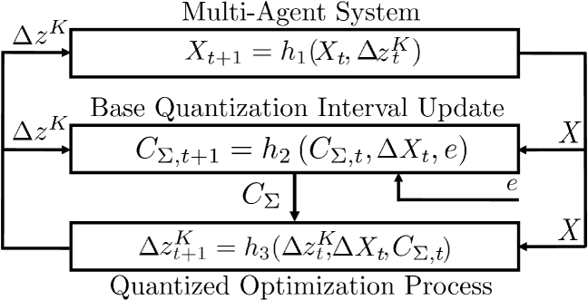
Figure 2: The interconnection of the three subsystems.

In order to carry out stability analysis using the small-gain theorem, we propose to consider the MAS (51) controlled by Alg. 2 as three interconnected subsystems, including the sub-optimally controlled MAS, the base quantization interval update process, and the quantized optimization process, as shown in Fig. 2. Their states are the state of the MAS $X_{t}$, the sum of base quantization interval $C_{\Sigma,t}$, and the sub-optimality of the optimization algorithm $\Delta z^{K}_{t}$, respectively. The parameter $e$ from (56) enters Subsystem 2 as an external input.

Subsystem 1. Given the DMPC problem (52) and Alg. 2, the dynamics of the sub-optimally controlled MAS is formulated as

$$X_{t+1} =h_{1}(X_{t},\Delta z^{K}_{t})$$

$$:=AX_{t}+B\Xi z^{K}_{t}=AX_{t}+B\Xi z^{*}_{t}+B\Xi\Delta z^{K}_{t},$$ (84)

where $B\Xi\Delta z^{K}_{t}$ represents a virtual perturbation resulted from the sub-optimality associated with $z^{K}_{t}$.

Subsystem 2. The dynamics of the base quantization interval update process in Step 5 and 6 of Alg. 2 is formulated as

$$C_{\Sigma,t+1} =h_{2}(C_{\Sigma,t},\Delta X_{t},e)$$

$$:=b_{1}C_{\Sigma,t}+b_{2}\sum_{i\in\mathcal{M}}\|\Delta\hat{X}_{i,t}\|+M(b_{3}+b_{4}b_{5})e,$$ (85)

which corresponds to the sum of updates in (63).

Subsystem 3. The dynamics of the quantized distributed optimization process formed by Step 5-8 of Alg. 2 is formulated as

$$\Delta z^{K}_{t+1}=h_{3}(\Delta z^{K}_{t},\Delta X_{t},C_{\Sigma,t}),$$ (86)

which corresponds the sub-optimality bound in (8) for time step $t+1$.

Next, we identify ISS-Lyapunov functions for the subsystems, and derive conditions on $n$ and $K$ for satisfying the small-gain conditions (4) and guaranteeing stability of the interconnected system.

V-C ISS-Lyapunov Functions for Subsystem 1, 2, and 3

Inspired by [9], we prove $\psi(X_{t}):=\sqrt{V(X_{t})}$ is an ISS-Lyapunov function for Subsystem 1. We also show $C_{\Sigma,t}$ and $\|{\Delta z^{K}_{t}}\|$ are ISS-Lyapunov functions for Subsystems 2 and 3, respectively, if $n$ and $K$ satisfy certain conditions. We present proofs of Propositions 2-4, and Theorem 1 in the Appendix.

Proposition 2 (ISS-Lyapunov Function for Subsystem 1).

Consider Subsystem 1 in (84) with an feasible initial state $X_{0}$. Suppose Assumptions 1-5 and Proposition 1 hold. Then, $\psi(X_{t})$ is an ISS-Lyapunov function of (84) satisfying

$$\psi(X_{t+1})\leq(1-\alpha_{1})\psi(X_{t})+\gamma_{1,3}\|{\Delta z^{K}_{t}}\|,$$ (87)

with $\alpha_{1}:=1-\sqrt{1-{\underline{\lambda}(Q)}/({L^{2}\overline{\lambda}(H)}})$ and $\gamma_{1,3}:=\sqrt{\overline{\lambda}(H)}\|B\|L$.

The difference between Proposition 2 and Theorem 1 in [9] is we define the Lipschitz constant $L$ differently in (55). The bound in Lemma 3 on $\Delta X_{t}$ is used in the proofs of Propositions 3 and 4.

Lemma 3 (Lemma 6, [21]).

Consider the MAS (51) controlled by $\pi^{K}(X_{t})$ defined in (54). The change in the state $\Delta X_{t}:=X_{t+1}-X_{t}$ of the MAS satisfies

$$\|\Delta X_{t}\|\leq c_{1}\psi(X_{t})+\|B\|\|{\Delta z^{K}_{t}}\|,$$ (88)

where $c_{1}:=({\|A-I\|+\|B\|}){\sqrt{\underline{\lambda}(H)}}$.

Proposition 3 (ISS-Lyapunov Function for Subsystem 2).

Consider Subsystem 2 in (85). Suppose Assumptions 1-5 and Proposition 1 hold. If $n$ and $K$ satisfy

$$K\geq K_{1}:=\left\lceil-\log_{\rho}\left(\frac{1-Ma_{2}}{Ma_{1}a_{3}+1-Ma_{2}}\right)\right\rceil,$$ (89)

where $a_{1}$-$a_{3}$ in (9) depend on $n$, then $C_{\Sigma,t}$ is an ISS-Lyapunov of (85) satisfying

$${C_{\Sigma,t+1}\leq(1-\alpha_{2})C_{\Sigma,t}+\max(\gamma_{2,1}\psi(X_{t}),\gamma_{2,3}\|{\Delta z^{K}_{t}}\|,\gamma^{e}_{2}e),}$$ (90)

where $\alpha_{2}:=1-b_{1}$, $\gamma_{2,1}:=3b_{2}Mc_{1}$, $\gamma_{2,3}:=3M\|B\|b_{2}$, and $\gamma^{e}_{2}:=3M(4b_{2}+b_{3}+b_{4}b_{5})$.

Proposition 4 (ISS-Lyapunov Function for Subsystem 3).

Consider Subsystem 3 in (86). Suppose Assumptions 1-5 and Proposition 1 hold. If $n$ and $K$ satisfy

$$K\geq K_{2}:=\left\lceil-\log_{\rho}\left(c_{2}\right)\right\rceil,$$ (91)

where $c_{2}:={1}/({1+L\|B\|+a_{3}M\|B\|b_{2}})$, with $a_{3}$ in (9) and $b_{2}$ in (57) depending on $n$, then $\|{\Delta z^{K}_{t}}\|$ is an ISS-Lyapunov function of (86) satisfying

$$\|{\Delta z^{K}_{t+1}}\|\leq(1-\alpha_{3})\|{\Delta z^{K}_{t}}\|+\max(\gamma_{3,1}\psi(X_{t}),\gamma_{3,2}C_{\Sigma,t},\gamma^{e}_{3}e),$$ (92)

where $\alpha_{3}:=1-\rho^{2K}/b_{1}$, $\gamma_{3,1}:=3\rho^{K}(L+Mb_{2})c_{1}$, $\gamma_{3,2}:=3\rho^{K}a_{3}b_{1}$, and $\gamma^{e}_{3}:=\gamma^{e}_{2}$.

V-D Conditions on the Quantization Parameters for Stability

We now derive conditions on $n$ and $K$, given $T$, such that the three interconnected cycles in Fig. 2 satisfy the small-gain conditions (4) which further implies stability of the interconnected system. Let $\mathcal{X}_{i,j}:=\tilde{\alpha}_{i}^{-1}\circ\left(\mathrm{Id}-\tilde{\mu}_{i}\right)^{-1}\circ\tilde{\gamma}_{i,j},\;i\in\{1,2,3\}$, with

$$\tilde{\alpha}_{1}(s):=\alpha_{1}s,\;\;\;\;\;\tilde{\alpha}_{2}(s):=\alpha_{2}s,\;\;\;\;\;\tilde{\alpha}_{3}(s):=\alpha_{3}s,$$

$$\tilde{\gamma}_{1,3}(s):={\gamma}_{1,3}s,\;\tilde{\gamma}_{2,1}(s):={\gamma}_{2,1}s,\;\tilde{\gamma}_{2,3}(s):={\gamma}_{2,3}s,$$

$$\tilde{\gamma}_{3,1}(s):={\gamma}_{3,1}s,\;\tilde{\gamma}_{3,2}(s):={\gamma}_{3,2}s,$$

the small-gain conditions corresponding to the three cycles are: there exist $\tilde{\mu}_{i},i\in\{1,2,3\}$ such that

$$\mathcal{X}_{1,3}\circ\mathcal{X}_{3,1} <\text{Id},\allowdisplaybreaks$$ (93a)

$$\mathcal{X}_{2,3}\circ\mathcal{X}_{3,2} <\text{Id},\allowdisplaybreaks$$ (93b)

$$\mathcal{X}_{1,3}\circ\mathcal{X}_{3,2}\circ\mathcal{X}_{2,1} <\text{Id}.$$ (93c)

Theorem 1.

Consider the MAS (51) controlled by the DMPC framework in Alg. 2. Suppose Assumptions 1-5 hold. Given communication data rate $T$ defined as the number of bits that can be transmitted per time step. If the quantization bit number $n$ and optimization iteration number $K$ satisfy $nK\leq T$, (6), (58), and

$$K\geq\max(K_{1},K_{2},K_{3},K_{4},K_{5}),$$ (94)

where $K_{1}$ defined (89), $K_{2}$ defined in (91), and

$$K_{3}:={\left\lceil\operatorname{log}_{\rho}\left(\frac{\alpha_{1}-3M{\gamma}_{1,3}b_{2}c_{1}}{3L{\gamma}_{1,3}c_{1}+\alpha_{1}c_{2})}\right)\right\rceil},\allowdisplaybreaks$$ (95a)

$$K_{4}:=\left\lceil\operatorname{log}_{\rho}\left(\frac{-\bar{b}_{1}+\sqrt{\bar{b}^{2}_{1}-4\bar{a}_{1}\bar{c}_{1}}}{2\bar{a}_{1}}\right)\right\rceil,\allowdisplaybreaks$$ (95b)

$$K_{5}:=\left\lceil\operatorname{log}_{\rho}\left(\frac{-\bar{b}_{2}+\sqrt{\bar{b}^{2}_{2}-4\bar{a}_{2}\bar{c}_{2}}}{2\bar{a}_{2}}\right)\right\rceil,\allowdisplaybreaks$$ (95c)

depend on $n$, with

$$\bar{a}_{1}:=\frac{{\rho^{K}}c_{2}-{b_{1}}}{{3{\rho^{K}}\gamma}_{2,3}a_{3}},\bar{b}_{1}:=\frac{-{\rho^{K}}-{b_{1}}c_{2}}{{3{\rho^{K}}\gamma}_{2,3}a_{3}},\bar{c}_{1}:=\frac{{b_{1}}}{{3{\rho^{K}}\gamma}_{2,3}a_{3}},$$

$$\bar{a}_{2}:=\frac{{\rho^{K}}\alpha_{1}c_{2}}{3{\gamma}_{1,2}{\gamma}_{2,3}{b_{1}}c_{1}},\bar{b}_{2}:=\frac{-{\rho^{K}}\alpha_{1}-\alpha_{1}{b_{1}}c_{2}-L{b_{1}}}{3{\gamma}_{1,2}{\gamma}_{2,3}{b_{1}}c_{1}},$$

$$\bar{c}_{2}:=\frac{\alpha_{1}}{3{\gamma}_{1,2}{\gamma}_{2,3}c_{1}}-Mb_{2},$$

then the MAS (51) controlled by Alg. 2 is recursively feasible and the closed-loop system is ISS w.r.t the parameter $e$ in (56) considered as a constant external input.

Remark 3.

If $e=0$ as a result of, i.e. all agents having accurate estimates of the global state (the network has a central node), the interconnected system becomes asymptotically stable.

Remark 4.

The small-gain conditions (93) naturally embed a degree of conservatism. [jiang_necessary] proved small-gain-type conditions as necessary (tight) and sufficient for a family of interconnected systems. Extending this result to our problem setting can be a future direction. Bad estimation of Lipschitz constants may also lead to conservatism in the bound (94) since the value of $\max(K_{1},\allowbreak K_{2},\allowbreak K_{3},\allowbreak K_{4},\allowbreak K_{5})$ depends on $L_{i}$, $L_{f}$, and $L$. To reduce $L$, pre-conditioning the optimization problem underlying (52) is viable [9]. At the cost of potentially reduced closed-loop performance, one can also tune the DMPC problem parameters (e.g., $H_{i}$ and $P_{i}$ in (52a)) and adjust the network topology (e.g. reducing degree $d$ of $\mathcal{G}$) to reduce $L_{i}$, $L_{f}$, and $L$.

Remark 5.

Given a limited data rate $T$, it is possible a combination of $n$ and $K$ satisfying $nK\leq T$, (6), (58), and (94) does not exist. In this case, one can solve the quantization parameter design problem:

$$T_{\min}=\underset{n,K\in\mathbb{Z}_{+}}{{\min}}nK,\text{ s.t. }\eqref{n definition},\eqref{n definition 2},\eqref{final condition on K}.$$ (96)

to determine the minimum data rate $T_{\min}$ required to implement Alg. 2 with closed-loop stability guarantee. Note that (96) is solvable off-line through enumeration.

VI Multi-AUV Formation Control Problem

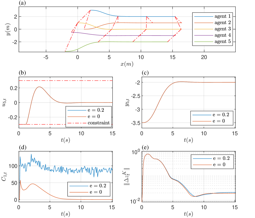
Figure 3: (a) the trajectories of the AUVs; (b) the input $u_{5,t}$ of AUV 5; (c)-(e) the change in $y_{5,t}$, $C_{1,t}$, and $\|{\Delta z^{K}_{t}}\|$ w.r.t. time step $t$.

We demonstrate the proposed algorithm and the theoretical findings using a control example with multiple autonomous underwater vehicles (AUVs), which suffers from limited underwater communication data rate. There are five AUVs moving in the $xy$-plane (horizontal) and communicating according the neighbourhoods $\mathcal{N}_{1}=\{1,2,3\}$, $\mathcal{N}_{2}=\{1,2\}$, $\mathcal{N}_{3}=\{1,3,4\}$, $\mathcal{N}_{4}=\{3,4\}$, and $\mathcal{N}_{5}=\{3,5\}$. The MAS is controlled by a $y$-axis controller based on Alg. 2, which we focus on, and a low-level $x$-axis controller. The AUV dynamics in the $y$-axis is $\zeta_{i,t+1}=A_{i}\zeta_{i,t}+B_{i}u_{i,t}$, where $\zeta_{i}:=[y_{i},\delta_{i},\omega_{i}]^{\top}$ and

$$A_{i}=\begin{bmatrix}1&T_{d}v_{c}&0\\ 0&1&T_{d}\\ 0&0&1-{N_{\omega}}/{\mathcal{I}}\end{bmatrix},\;B_{i}=\begin{bmatrix}0\\ 0\\ {1}/{\mathcal{I}}\end{bmatrix},$$

with position $-5\leq y_{i}\leq 5$ m, yaw angle $-1\leq\delta_{i}\leq 1$ rad, angular velocity $-2\leq\omega_{i}\leq 2$ rad/s, input torque $-0.3\leq u_{i}\leq 0.3$ N$\cdot$m/s, velocity $v_{c}=1$ m/s, rotational inertia $\mathcal{I}=2$ kg$\cdot$m², damping coefficient $N_{\omega}\allowbreak=\allowbreak 1$ N$\cdot$m/(rad/s), and sampling time $T_{d}=0.1$ s. This constraint setup satisfies Assumption 1. The initial states of the AUVs are $[y_{1,0},\allowbreak y_{2,0},\allowbreak y_{3,0},\allowbreak y_{4,0},\allowbreak y_{5,0}]^{\top}=[5,\allowbreak 0,\allowbreak 1,\allowbreak-0.5,\allowbreak-3.5\allowbreak]^{\top}$ m, $\delta_{i,0}=0$ rad, and $\omega_{i,0}=0$ rad/s, $\forall i\in\{1,\cdots,5\}$. Their reference states are $[y_{r,1},\allowbreak y_{r,2},y_{r,3},\allowbreak y_{r,4},\allowbreak y_{r,5}]^{\top}=\allowbreak[2,\allowbreak 1,\allowbreak 0,\allowbreak-1,\allowbreak-2]^{\top}$ m, $\delta_{r,i}=0$ rad, and $\omega_{r,i}=0$ rad/s, $\forall i\in\{1,\cdots,5\}$. The DMPC formulation in Section III-A of [15] is implemented, which imposes penalty on the relative $y$-distance errors between AUVs $i$ and $j$, $\forall j\in\mathcal{N}_{i}$. Choosing $N=18$, $Q_{i},\allowbreak R_{i},\allowbreak S_{ij}\in I$, $P_{i}$, $K_{f,i}$ satisfying Assumption 3 is determined by solving the algebraic Ricatti inequality and enforcing appropriate constraints on $P$ to ensure a separable structure. Local terminal constraint $\mathcal{C}_{f,i}:=\{\zeta_{i}\mid\|\zeta_{i}\|^{2}_{P_{i}}\leq 0.057\}$ are determined through ellipsoidal approximation. Since the local cost functions depend $Q_{i}$, $S_{i}$, $R_{i}$, $P_{i}\in\mathbb{S}_{++}$, Assumption 2 is satisfied.

To obtain a Lipschitz constant satisfying Assumption 4, we uniformly sample global states $\zeta_{m}$ and inputs $u_{m}$ from the constraints and compute $\tilde{\zeta}_{m}=A\zeta_{m}+BU_{m}$. We collect 2000 pairs of $(\zeta_{m},\tilde{\zeta}_{m})$ that are both feasible for the DMPC problem. The Lipschitz constant $L=9.72$ is computed from $L=\max_{1\leq m\leq 2000}\frac{\|\zeta_{m}-\tilde{\zeta}_{m}\|}{\|z^{*}(\zeta_{m})-z^{*}(\tilde{\zeta}_{m})\|}$. Given $T=32$ kB/s, the parameters for Alg. 2 are chosen as $\rho=0.986$, $\eta=0.001$, $n=26$, and $K=1000$, where $n$ and $K$ satisfy conditions (6), (58), and (94).

We simulate and compare two cases: with and without estimation noise. For the first case, we sample $e_{i,t}$ uniformly from $[-0.05,0.05]$ and set $e=0.2$ to satisfy Assumption 5. For the second case, we set $e=0$. Fig. 3(a) shows trajectories of the AUVs controlled by Alg. 2 with $e=0.2$, where the red dashed lines represent the current formation. It can be seen the AUVs converge to the references while forming the desired formation. Fig. 3(b) shows the input $u_{5,t}$ of AUV 5, where the input constraint $-0.3$ N$\cdot$m/s is activated before $t=1.3$ s. Fig. 3(c) shows the convergence of the position $y_{5,t}$ of AUV 5 (part of the state of Subsystem 1) to the reference state $y_{r,5}=-2$ m. Fig. 3(d) shows the evolution of $C_{1,t}$ (part of the state of Subsystem 2), which converges to a neighbourhood of $0$ when $e=0.2$ and to $0$ when $e=0$. Fig. 3(e) shows $\|{\Delta z^{K}_{t}}\|$ (normed state of Subsystem 3) converges to a plateau near $10^{-2}$ in both cases, which results from limited solver accuracy in the projection step of Alg. 1. After $t=5$ s, the value of $\|{\Delta z^{K}_{t}}\|$ with $e=0.2$ is slightly higher than that with $e=0$. As can be seen, the effect of the parameter $e$ is most obvious on the base quantization interval (Subsystem 2) and least visible in the state (Subsystem 1). This is expected since $e$ enters Subsystem 2 as a constant external input and its effect indirectly propagates through Subsystem 3 to Subsystem 1, as illustrated in Fig. 2. To conclude, the simulation results demonstrated that for a given data rate $T$, if the quantization bit number $n$ and iteration number $K$ satisfy the conditions in Theorem 1, then, the interconnected system formed by (84)-(86) is ISS w.r.t. the parameter $e$ considered as an external input.

VII Conclusions

We proposed a novel real-time DMPC framework with a quantization refinement scheme for MASs with limited communication data rates and derived sufficient conditions on the quantization parameters for guaranteeing the closed-loop stability. Future works can focus on quantitative methods for jointly designing the DMPC formulations (e.g., cost functions) and the algorithm parameters (e.g., $n$, $K$) to reduce the required communication data rate for guaranteeing closed-loop stability while maintaining certain level of performance. Another direction is to address the conservatism resulted from bounding $e_{i,t}$ with $e$, by developing an ISS-Lyapunov function for the estimation error $e_{i,t}$ w.r.t. the change in state $\Delta X_{t}$. This would enable us to consider the state estimation dynamics as another subsystem interconnected with the subsystems in (84)-(86), and apply the small-gain theorem to prove asymptotically stable of the overall system.

Appendix

VII-A Proof of Proposition 2

From Proposition 1, $X_{t}$ is feasible and $\pi^{K}(X_{t})$ and $\pi^{*}(X_{t})$ exist $\forall t\geq 0$. Let $X_{t+1}=AX_{t}+B\pi^{K}(X_{t})$, $\breve{X}_{t+1}=AX_{t}+B\pi^{*}(X_{t})$, $\psi(X_{t+1}):=\|z^{*}_{t+1}\|_{H}$, $\psi(\breve{X}_{t+1}):=\|\breve{z}^{*}_{t+1}\|_{H}$, we know that

$$\psi(X_{t+1})\leq|\|z^{*}_{t+1}\|_{H}-\|\breve{z}^{*}_{t+1}\|_{H}|+\|\breve{z}^{*}_{t+1}\|_{H}.$$ (97)

From Assumption 3, we have

$$V(\breve{X}_{t+1})\leq V(X_{t})-\|X_{t}\|^{2}_{Q}.$$ (98)

Lower bounding $\|X_{t}\|^{2}_{Q}$ with

$$\|X_{t}\|^{2}_{Q}\geq\underline{\lambda}(Q)\|X_{t}\|^{2}\overset{\eqref{existence of L}}{\geq}\frac{\underline{\lambda}(Q)}{L^{2}}\|z^{*}_{t}\|^{2}\geq\frac{\underline{\lambda}(Q)}{L^{2}\overline{\lambda}(H)}\|z^{*}_{t}\|^{2}_{H},$$

and then taking square-roots on both sides of (98) yields

$$\psi(\breve{X}_{t+1})\leq\sqrt{1-{\underline{\lambda}(Q)}/({L^{2}\overline{\lambda}(H)})}\psi(X_{t}).$$ (99)

Applying the reverse triangle inequality, we have

$$|\|z^{*}_{t+1}\|_{H}-\|\breve{z}^{*}_{t+1}\|_{H}|^{2}\leq\|z^{*}_{t+1}-\breve{z}^{*}_{t+1}\|^{2}_{H}\allowdisplaybreaks$$

$$\;\;\;\;\;\leq\overline{\lambda}(H)\|z^{*}_{t+1}-\breve{z}^{*}_{t+1}\|^{2}\overset{\eqref{existence of L}}{\leq}\overline{\lambda}(H)L^{2}\|X^{*}_{t+1}-\breve{X}^{*}_{t+1}\|^{2}.\allowdisplaybreaks$$ (100)

Taking square-roots on both sides, we obtain

$$|\|z^{*}_{t+1}\|_{H}-\|\breve{z}^{*}_{t+1}\|_{H}|\leq\sqrt{\overline{\lambda}(H)}L\|X^{*}_{t+1}-\breve{X}^{*}_{t+1}\|$$

$$\leq\sqrt{\overline{\lambda}(H)}L\|B(\pi^{*}(X_{t})-\pi^{K}(X_{t}))\|\leq\sqrt{\overline{\lambda}(H)}L\|B\|\|{\Delta z^{K}_{t}}\|.$$ (101)

Then, bounding the r.h.s of (97) with (99) and (101) gives

$$\psi(X_{t+1})\leq(1-\alpha_{1})\psi(X_{t})+\gamma_{1,3}\|{\Delta z^{K}_{t}}\|,$$ (102)

where $\alpha_{1}=1-\sqrt{1-{\underline{\lambda}(Q)}/({L^{2}\overline{\lambda}(H)})}$ and $\gamma_{1,3}=\sqrt{\overline{\lambda}(H)}\|B\|L$. Since $\|z^{*}\|\leq L\|X\|$ from (55) and $\|z^{*}\|=\|[\textbf{X}^{*\top},\mathbf{U}^{*\top}]^{\top}\|\geq\|\mathrm{X}^{*}(0)\|=\|X\|$, we know $L\geq 1$. Further, since $\overline{\lambda}(H)\geq\underline{\lambda}(Q)$, we know that $\alpha_{1}\in(0,1)$. By definition, we also know $\gamma_{1,3}>0$. Therefore, $\psi(X_{t})$ is an ISS-Lyapunov function for Subsystem 1. $\blacksquare$

VII-B Proof of Proposition 3

Combining (62) with (88) gives

$$\|\Delta\hat{X}_{i,t-1}\|\leq c_{1}\psi(X_{t})+\|B\|\|{\Delta z^{K}_{t}}\|+2e.$$ (103)

Bounding $\|\Delta\hat{X}_{i,t-1}\|$ in (65) with (103) and doing simplification give

$$C_{\Sigma,t+1}\leq b_{1}C_{\Sigma,t}+Mb_{2}c_{1}\psi(X_{t})$$

$$+M\|B\|b_{2}\|{\Delta z^{K}_{t}}\|+M(4b_{2}+b_{3}+b_{4}b_{5})e$$ (104)

$$\leq(1-\alpha_{2})C_{\Sigma,t}+\max\left(\gamma_{2,1}\psi(X_{t}),\gamma_{2,3}\|{\Delta z^{K}_{t}}\|,\gamma^{e}_{2}e\right).$$ (105)

Since $\alpha_{2}\in(0,1)$ from (91) and $\gamma_{2,1},\gamma_{2,3},\gamma^{e}_{2}>0$ by definition, $C_{\Sigma,t}$ is an ISS-Lyapunov function for Subsystem 2. $\blacksquare$

VII-C Proof of Proposition 4

From Proposition 1, $n$ satisfies (6), (8) holds, and we have

$$\|{\Delta z^{K}_{t+1}}\|\overset{\eqref{rho to epsilon bound}}{\leq} \rho^{K}((\|{\Delta z^{K}_{t}}\|+L\|\Delta X_{t}\|)+a_{3}C_{\Sigma,t+1}).$$ (106)

Then, bounding $\|\Delta X_{t}\|$ with (88) and $C_{\Sigma,t+1}$ with (104) gives

$$\|{\Delta z^{K}_{t+1}}\|\leq\rho^{K}(1+L\|B\|+a_{3}M\|B\|b_{2})\|{\Delta z^{K}_{t}}\|+\rho^{K}a_{3}b_{1}C_{\Sigma,t}$$

$$\;\;\;+\gamma_{3,1}(L+Mb_{2})c_{1}\psi(X_{t})+M(4b_{2}+b_{3}+b_{4}b_{5})e$$ (107)

$$\leq(1-\alpha_{3})\|{\Delta z^{K}_{t}}\|+\max\left(\gamma_{3,1}\psi(X_{t}),\gamma_{3,2}C_{\Sigma,t},\gamma^{e}_{3}e\right).$$ (108)

Since $\alpha_{3}\in(0,1)$ from (91) and $\gamma_{3,1},\gamma_{3,2},\gamma^{e}_{3}>0$ by definition, $\|{\Delta z^{K}_{t}}\|$ is an ISS-Lyapunov function for Subsystem 3. $\blacksquare$

VII-D Proof of Theorem 1

Since the initial state $X_{0}$ is feasible and $n$ satisfies (6) and (58), the MAS (51) under Alg. 2 is recursively feasible (Proposition 1).

Since Assumptions 1-5 hold, the quantization bit number $n$ and iteration number $K$ satisfy (6), (58), and $K\geq\max(K_{1},K_{2})$, it is ensured Propositions 2-4 hold, i.e., Subsystems 1-3 admit (87), (90), and (92) as ISS-Lyapunov functions, respectively.

In addition, since the iteration number also satisfies $K\geq\max(K_{3},K_{4},K_{5})$, the following conditions hold:

$$\tilde{\alpha}_{1}^{-1}\circ\tilde{\alpha}_{3}^{-1}\circ\tilde{\gamma}_{1,3}\circ\tilde{\gamma}_{3,1} <\textup{Id},$$

$$\tilde{\alpha}_{2}^{-1}\circ\tilde{\alpha}_{3}^{-1}\circ\tilde{\gamma}_{2,3}\circ\tilde{\gamma}_{3,2} <\textup{Id},$$

$$\tilde{\alpha}_{1}^{-1}\circ\tilde{\alpha}_{2}^{-1}\circ\tilde{\alpha}_{3}^{-1}\circ\tilde{\gamma}_{1,3}\circ\tilde{\gamma}_{3,2}\circ\tilde{\gamma}_{2,1} <\textup{Id},$$

which implies there always exist linear gain functions $\tilde{\mu}_{i}(s):={\mu}_{i}s$, with $\mu_{i}>0$, $i\in\{1,2,3\}$, such that the small-gain conditions in (93) hold, i.e., $\mathcal{X}_{1,3}\circ\mathcal{X}_{3,1}<\text{Id}$, $\mathcal{X}_{2,3}\circ\mathcal{X}_{3,2}<\text{Id}$, and $\mathcal{X}_{1,3}\circ\mathcal{X}_{3,2}\circ\mathcal{X}_{2,1}<\text{Id}$, where $\mathcal{X}_{i,j}:=\tilde{\alpha}_{i}^{-1}\circ\left(\mathrm{Id}-\tilde{\mu}_{i}\right)^{-1}\circ\tilde{\gamma}_{i,j}$. Therefore, the interconnected system formed by (84)-(86) is ISS w.r.t the parameter $e$ considered as a constant external input. $\blacksquare$

References

- [1] S. E. Li, Y. Zheng, K. Li, Y. Wu, J. K. Hedrick, F. Gao, and H. Zhang, “Dynamical modeling and distributed control of connected and automated vehicles: Challenges and opportunities,” IEEE Intelligent Transportation Systems Magazine, vol. 9, no. 3, pp. 46–58, 2017.
- [2] Y. Pu, M. N. Zeilinger, and C. N. Jones, “Quantization design for distributed optimization,” IEEE Trans. on Auto. Control, vol. 62, no. 5, pp. 2107–2120, 2017.
- [3] S. Magnússon, H. Shokri-Ghadikolaei, and N. Li, “On maintaining linear convergence of distributed learning and optimization under limited communication,” IEEE Trans. on Signal Processing, vol. 68, pp. 6101–6116, 2020.
- [4] P. Scokaert, D. Mayne, and J. Rawlings, “Suboptimal model predictive control (feasibility implies stability),” IEEE Transactions on Automatic Control, vol. 44, no. 3, pp. 648–654, 1999.
- [5] M. N. Zeilinger, C. N. Jones, D. M. Raimondo, and M. Morari, “Real-time mpc - stability through robust mpc design,” in Proceedings of the 48h IEEE Conference on Decision and Control (CDC), 2009, pp. 3980–3986.
- [6] M. N. Zeilinger, D. M. Raimondo, A. Domahidi, M. Morari, and C. N. Jones, “On real-time robust model predictive control,” Auto.a, vol. 50, no. 3, pp. 683–694, 2014.
- [7] S. Richter, C. N. Jones, and M. Morari, “Computational complexity certification for real-time mpc with input constraints based on the fast gradient method,” IEEE Trans. on Auto. Control, vol. 57, no. 6, pp. 1391–1403, 2012.
- [8] A. Zanelli, Q. Tran-Dinh, and M. Diehl, “A lyapunov function for the combined system-optimizer dynamics in inexact model predictive control,” Auto.a, vol. 134, p. 109901, 2021.
- [9] D. Liao-Mc Pherson, T. Skibik, J. Leung, I. V. Kolmanovsky, and M. M. Nicotra, “An analysis of closed-loop stability for linear model predictive control based on time-distributed optimization,” IEEE Trans. on Auto. Control, pp. 1–1, 2021.
- [10] T. Liu, Z. Qin, Y. Hong, and Z.-P. Jiang, “Distributed optimization of nonlinear multiagent systems: A small-gain approach,” IEEE Transactions on Automatic Control, vol. 67, no. 2, pp. 676–691, 2022.
- [11] P. Giselsson and A. Rantzer, “Distributed model predictive control with suboptimality and stability guarantees,” in 49th IEEE Conference on Decision and Control (CDC), 2010, pp. 7272–7277.
- [12] ——, “On feasibility, stability and performance in distributed model predictive control,” IEEE Trans. on Auto. Control, vol. 59, pp. 1031–1036, 2014.
- [13] S. El-Ferik, B. A. Siddiqui, and F. L. Lewis, “Distributed nonlinear mpc of multi-agent systems with data compression and random delays,” IEEE Trans. on Auto. Control, vol. 61, no. 3, pp. 817–822, 2016.
- [14] R. E. Jalal and B. P. Rasmussen, “Limited-communication distributed model predictive control for coupled and constrained subsystems,” IEEE Trans. on Control Systems Technology, vol. 25, no. 5, pp. 1807–1815, 2017.
- [15] Y. Yang, Y. Wang, C. Manzie, and Y. Pu, “Real-time distributed mpc for multiple underwater vehicles with limited communication data-rates,” in 2021 American Control Conference (ACC), 2021, pp. 3314–3319.
- [16] T. Liu, D. J. Hill, and Z.-P. Jiang, “Lyapunov formulation of the large-scale, iss cyclic-small-gain theorem: The discrete-time case,” Systems and Control Letters, vol. 61, no. 1, pp. 266–272, 2012.
- [17] W. W. Hager, “Lipschitz continuity for constrained processes,” SIAM Journal on Control and Optimization, vol. 17, no. 3, pp. 321–338, 1979.
- [18] M. S. Darup, M. Jost, G. Pannocchia, and M. Mönnigmann, “On the maximal controller gain in linear mpc,” IFAC-PapersOnLine, vol. 50, no. 1, pp. 9218–9223, 2017.
- [19] F. C. Rego, Y. Pu, A. Alessandretti, A. P. Aguiar, A. M. Pascoal, and C. N. Jones, “A distributed luenberger observer for linear state feedback systems with quantized and rate-limited communications,” IEEE Trans. on Auto. Control, vol. 66, no. 9, pp. 3922–3937, 2021.
- [20] L. Rong, S. Wang, G.-P. Jiang, and S. Xu, “Distributed observer-based consensus over directed networks with limited communication bandwidth constraints,” IEEE Trans. on Systems, Man, and Cybernetics: Systems, vol. 50, no. 12, pp. 5361–5368, 2020.
- [21] J. Leung, D. Liao-McPherson, and I. V. Kolmanovsky, “A computable plant-optimizer region of attraction estimate for time-distributed linear model predictive control,” in 2021 American Control Conference (ACC), 2021, pp. 3384–3391.