Deformation equivariant cross-modality image synthesis with paired non-aligned training data

Abstract

Cross-modality image synthesis is an active research topic with multiple medical clinically relevant applications. Recently, methods allowing training with paired but misaligned data have started to emerge. However, no robust and well-performing methods applicable to a wide range of real world data sets exist. In this work, we propose a generic solution to the problem of cross-modality image synthesis with paired but non-aligned data by introducing new deformation equivariance encouraging loss functions. The method consists of joint training of an image synthesis network together with separate registration networks and allows adversarial training conditioned on the input even with misaligned data. The work lowers the bar for new clinical applications by allowing effortless training of cross-modality image synthesis networks for more difficult data sets.

1 Introduction

Image-to-image translation is an active area of research in computer vision because of its various applications such as image synthesis, segmentation, restoration, style transformation and pose estimation. After the advent of deep leaning, medical imaging as a cardinal application area, has seen an increasing interest in the use of image-to-image translation. In histopathology, image-to-image translation has been used, e.g., for cross-stain translation [39, 63], for replacing chemical staining by digitally generated mask [55], for tissue color normalization [14, 7], for virtual staining of label-free or unstained tissue images [6, 45, 47]. In radiology, it has been used for pseudo CT generation and cross-modality MRI synthesis, and the synthesized images have been shown to be useful for downstream tasks, e.g., segmentation [9, 50, 62]. The image-to-image translation methods are primarily divided into two categories: supervised methods that rely upon aligned image pairs and unsupervised methods that don’t require aligned image pairs. In the medical setting including supervision tends to improve the results [23, 29, 37, 43, 16].

Image-to-image translation is called differently depending on the application and in this work we will call it cross-modality image synthesis, which is often used in the medical imaging context. We use the term modality broadly to refer to any distinct image types capturing different characteristics of the underlying anatomy.

In the medical domain, different modality images of the same subject are not usually anatomically aligned. To solve this before training a network images are typically registered, or in other words, aligned anatomically. Deep learning registration methods have gained popularity [17] with the best methods performing close to classical registration algorithms, e.g. in Learn2Reg multi-task medical image registation challenge [18] or in histopathology ANHIR competition [8].

Methods combining the two, cross-modality image synthesis and cross-modality registration, have also started to surface. In registration a synthesized image can be used as a bridge to generate a cross-modality similarity metric [40]. However, some methods combine these two into a unified architecture, solving both problems at the same time. Such methods have been published from both the registration [1, 12] and image synthesis viewpoint [24, 32, 57, 58, 59].

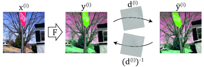
Figure 1: Basic setting. Only non-aligned pairs of $x^{(i)}$ and $\tilde{y}^{(i)}$ are available but the task is to learn $F$ for transforming $x^{(i)}$ into $y^{(i)}$. The images are from the synthetic ”multimodal” data sets built using COCO [38] data set.

In this paper, we propose a new architecture for cross-modality image synthesis which is robustly trainable with misaligned training data, using a novel strategy that couples registration and image synthesis networks during training. Firstly, we suggest training the image-synthesis network directly for deformation equivariance which refers to the property that applying a deformation before or after the image synthesis should result in the same image. Secondly, we develop a strategy allowing adversarial training conditioned on the input images despite using misaligned training data, not possible to do robustly by earlier methods. Conditioning adversarial training on the input is especially important in the medical domain as it results in more reliable predictions. In addition to the better quality predictions the method is applicable to a wider range of data sets than earlier similar methods. In the experiments we show that the method improves upon earlier methods trainable on non-aligned data and that it also surpasses the standard approach where the images are registered before training, assuming that no significant manual effort is put into the registration.

2 Basic Setting

Assume we have a paired training set of input images $(x^{(1)},\dots,x^{(N)})$ and non-aligned target images $(\tilde{y}^{(1)},\dots,\tilde{y}^{(N)})$. Following the notation by Kong et al. [32] we denote the (unavailable) aligned ground truth targets by $(y^{(1)},\dots,y^{(N)})$. Furthermore, unknown deformations $(d^{(1)},\dots,d^{(N)})$ connect the coordinate systems of the inputs and the targets.

Assuming that the images are continuous, they can be seen as mappings $x^{(i)}:\mathbb{R}^{n}\to\mathbb{R}^{m_{1}}$ and $y^{(i)},\tilde{y}^{(i)}:\mathbb{R}^{n}\to\mathbb{R}^{m_{2}}$ where $n$ is the dimensionality of the image (e.g. $n=2$ for two dimensional images) and $m_{1}$ and $m_{2}$ are number of channels in input and target images respectively (e.g. $3$ for RGB images). The deformations would then be mappings $d^{(i)}:\mathbb{R}^{n}\to\mathbb{R}^{n}$ connecting the image coordinates. Doing a coordinate transformation of an image $x^{(i)}$ based on a deformation $d^{(i)}$ would equal to function composition $x^{(i)}\circ d^{(i)}$ which can be written using the pullback notation as $d^{(i)*}x^{(i)}:=x^{(i)}\circ d^{(i)}$ where $d^{(i)*}$ can be seen as a mapping acting on images.

Following the notation, we have the relationship $d^{(i)*}y^{(i)}=\tilde{y}^{(i)}$ between the aligned and non-aligned targets. In practice, the images are not continuous, but instead only samples of the images are available, i.e. the pixels or voxels. Hence in reality, the mapping $d^{(i)*}$ equals to interpolating the image at the locations defined by the deformation, and we use linear interpolation.

In this work, we study a setting where we are trying to learn a function $F$ which is a neural network such that $F(x^{(i)})=y^{(i)}$. To do this, we simultaneously try to learn a second neural network, or, as it turns out, multiple networks, for predicting $d^{(i)}$. However, during test time we still only want to use the network $F$.

3 Previous Work

3.1 Cross-Modality Image Synthesis

Cross-modality medical image synthesis has gained a lot of attention in recent years with multiple proposed clinical applications [60]. The conditional GAN-based architecture pix2pix [22] is widely used when paired and aligned data are available as it is based on an assumption of pixel-to-pixel correspondence between training images of different modality. On the other hand, CycleGAN [66] can be used without paired or aligned data.

Paired training images in the medical context are typically not aligned, and hence for pixel-to-pixel training they are registered into the same coordinate system. However, registration is never perfect and pixel-to-pixel losses are very sensitive to registration errors reducing the synthesis quality especially on difficult to register areas with large internal anatomic motion such as on pelvis area [60].

In pixel-to-pixel setting, different approaches have been proposed to mitigate for the remaining registration errors [10, 24, 26, 36, 64]. Most similarly to our work, Kong et al. [32] combine a cross-modality image synthesis network with a registration network to enable training with non-aligned data. However, we argue that their method does not robustly mitigate for registration errors especially with real world data sets as will be dicussed in Section 4. Additionally they use unconditional adversarial training which has been shown to be inferior to conditioning the discriminator with input images. In this work we aim to solve both of these problems.

While performing worse than pix2pix when paired and aligned data are available, unsupervised CycleGAN is more robust against misalignments due to its cycle consistency loss [25, 60]. However, if the misalignments between the modalities are systematic and severe, CycleGAN can also fail to produce geometrically aligned predictions. Approaches, similar to ones used with pix2pix, have also been employed with CycleGAN [65, 20, 28]. Wang et al. [57, 58, 59] propose network architectures combining cross-modality image synthesis and registration, together with mutual information loss between the input and the prediction to promote similar geometry.

3.2 Cross-Modality Registration

Deformable medical image registration using deep learning has also gained popularity recently [17]. With stationary velocity field parametrization, one can generate diffeomorphic deformations [2, 3]. This kind of methodology was applied to deep learning by Dalca et al. [13]. Some architectures such as the one by De Vos et al. [15] combine affine or rigid registration together with a separate deformable registration resulting in multi-stage registration approach.

From cross-modality registration methods, the method by Arar et al. [1] is closest to our work. They train a cross-modality registration network by simultaneously training a cross-modality image synthesis network which they encourage to be equivariant to deformations predicted by the registration network. This is done by applying the predicted deformation both before and after the image synthesis network and comparing both of them to the target. We instead use simulated deformations for encouraging deformation equivariance. We argue that this leads to a more robust approach, which we verify in the experiments. Our method of encouraging deformation equivariance is similar to the method by Pielawski et al. [44] where they train their network for rotational equivariance.

Very recently, Chen et al. [12] use a contrastive learning based loss for promoting geometric (or shape) similarity of the image synthesis in an otherwise similar setting to Arar et al.

4 Methods

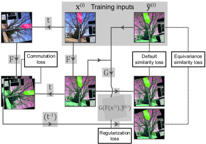
Figure 2: Proposed core architecture. When using the equivariance similarity loss instead of the default similarity loss, the commutation loss is optional. The architecture presented here is further refined by adding an adversarial loss and a separate cross-modality registration network for first registering $\tilde{y}^{(i)}$ to $x^{(i)}$. Deformation $t$ is a random deformation sampled on the fly individually for each training image pair. The images are from the synthetic ”multimodal” data sets built using COCO [38] data set.

To teach the network $F$ for predicting $y^{(i)}$ from $x^{(i)}$, Kong et al. [32] train an additional network $G$ aimed at learning the $d^{(i)}$ s.t. $G(F(x^{(i)}),\tilde{y}^{(i)})=d^{(i)}$. They train both of the networks $F$ and $G$ simultaneously with the similarity loss (which we label default similarity loss)

$$\mathcal{L}_{\text{def-sim}}:=\mathbb{E}_{x,\tilde{y}}||\tilde{y}-G(F(x),\tilde{y})^{*}F(x)||_{L^{1}}$$ (1)

together with a regularization loss

$$\mathcal{L}_{\text{reg}}:=\mathbb{E}_{x,\tilde{y}}\operatorname{Reg}(G(F(x),\tilde{y}))$$

where $\operatorname{Reg}$ is some operator penalizing non-smooth deformations, and an unconditional adversarial loss with the intent of training the distribution of $F(x^{(i)})$ to match the distribution of $\tilde{y}^{(i)}$.

In the work by Kong et al. they view the deformations between inputs and targets as noise and assume the same underling physical distribution for both the inputs and the targets. In that setting, the adversarial training objective they use is justified. However, often images in the target domain might be systematically geometrically different to the images in the input domain, e.g., when patients are laying differently within different medical imaging equipment. In that case matching the distribution of $F(x^{(i)})$ with the distribution of $\tilde{y}^{(i)}$ is not desirable.

To fix this we first omit the adversarial loss altogether, although we will develop a revised adversarial training strategy later. However, without the adversarial loss the optimization problem is very unstable since the network $F$ is not in any way constrained to preserve the geometry of the input images, that is, the predictions are not guaranteed to be anatomically aligned with the inputs. If $F$ is a convolutional neural network it has an inductive bias towards this kind of a behaviour but there is no guaranatee that the convolutional network does not, e.g., shift the predictions and the registration network compensate for the shift. An example of a possible failure mode is shown later in Figure 8. It is also noteworthy that while having the adversarial training in a setting similar to the work by [32] will definitely stabilize the training, there is no fundamental theoretical reason why it should result in $F$ preserving the geometry of its inputs.

The property of $F$ preserving the geometry of an input can be formulated as deformation equivariance. Any movement in the underlying anatomy of the input image should be reflected similarly in the output image. Assuming a set of anatomically possible geometric deformations $T^{(i)}$ for each input image $x^{(i)}$, a network $F$ is deformation equivariant over the deformations if for all $t\in T^{(i)}$ it holds that

$$t^{*}F(x^{(i)})=F(t^{*}x^{(i)}).$$ (2)

In other words, $F$ should commute with respect to the deformations of $x^{(i)}$.

In practice we do not aim for the relation to hold exactly but instead propose to promote the property implicitly by modifying the default similarity loss given in Equation (1). The modification is similar to the one by Pielawski et al. [44], although they use it in a different contrastive learning setting. We label the resulting loss equivariance similarity loss:

$$\mathcal{L}_{\text{eq-sim}}=\mathbb{E}_{x,\tilde{y},t}||\tilde{y}-(G(F(x),\tilde{y})^{*}t^{-1})^{*}F(t^{*}x)||_{L^{1}}$$ (3)

Here $t$ is seen as a random variable sampled from some distribution. The loss can be zero only if $F$ is equivariant to all $t$ and inputs. Note that we first compose the deformations $G(F(x),\tilde{y})$ and $t^{-1}$ and after that deform the prediction $F(t^{*}x)$. This way we avoid multiple interpolations of the same image. The same strategy of composing the deformations first is always used in this paper when applying multiple deformations to an image.

The loss in Equation 3 also acts as a data augmentation method by randomly transforming inputs fed into the network $F$. However, in contrast to the traditional data augmentation, we do not transform the target image with the same deformation as the input.

Optionally one can more directly promote the equivariance by training with the following objective which we label commutation loss:

$$\mathcal{L}_{\text{com}}:=\mathbb{E}_{x,t}||t^{*}F(x)-F(t^{*}x)||_{L^{1}}$$ (4)

When using the commutation loss using the equivariance similarity loss is optional and the default similarity loss can be used as well. Without the commutation loss the equivariance similarity loss is needed. As a result we have three possible configurations.

Arar et al. [1] also encourage deformation equivariance but only for deformations predicted by their registration network. That is not always enough, e.g., with perfectly aligned training data the network $F$ could still introduce any translation which the registration network could compensate since translations commute. Also with subtle systematic deformations the network $F$ might easily overlearn the deformations from the data resulting in the registration network predicting zero deformation. The limitations of their method are also discussed in the supplementary materials of their paper where they conclude that their method works only with relatively small image synthesis networks, which is not a large problem in their work which focuses on image registration, but a significant limitation in difficult cross-modality image synthesis tasks. Later, in Figure 10, we visualize a situation where our method succeeds in producing spatially aligned output but the method by Arar et al. [1] (NeMAR) fails.

The core architecture presented so far is visualized in Figure 2, and is in itself trainable. However, in addition to the core architecture, we will be looking at adding a conditional adversarial loss for training the model to improve the prediction quality further. In order for the adversarial training to converge even in the presence of systematically different geometries between the input and target domains, it turns out we will require two registration networks: one for registering targets to inputs and the other for registering predictions to possibly imperfectly registered targets.

Before advancing further, we introduce an additional notation. In case a variable should be treated as a constant from optimization point of view even if it is an output of a neural network, we overline the variable, e.g. $x^{(i)}$ vs. $\overline{x}^{(i)}$. In the neural network context, this means halting the backward pass during back-propagation.

4.1 Selecting a Set of Simulated Deformations

The equivariance similarity loss and the commutation loss require some way to simulate anatomically realistic deformations for calculating them. For promoting equivariance, an ideal set would be the set of all anatomically realistic deformations for each sample, but anatomically realistic non-affine deformations are very difficult to simulate. A natural question is then whether a significantly smaller set of deformations would be sufficient, especially considering the inductive biases of the used architectures.

Given that $F$ is a convolutional network it is (roughly) translation equivariant. Hence intuitively simulating only globally affine deformations might be enough since any diffeomorphic deformation is ”locally affine”. Also, affine deformations are easy to sample and the same distribution of deformations can be used for each sample. Applying affine deformations to images is also computationally efficient and numerically accurate. For these reasons we used only affine transformations in our experiments. It is left for future work to test whether elastic deformations could increase the performance further.

Affine transformations can be further divided into translation, rotation, scaling, shearing, and flipping. Translations and rotations should be reasonable to use in any practical situations, and flipping can be used when it doesn’t affect the distribution of the imaged anatomy. Scaling and shearing are more difficult since anatomically stretching a tissue could in principle affect its appearance under different imaging techniques. In other words, even in an ideal situation the deformation equivariance property would no longer hold exactly. In the experiments we conduct two studies on two data sets on using different types of affine transformations.

4.2 Adversarial Training

In addition to the losses presented so far, we want to incorporate adversarial loss to the training in order to improve the appearance and also clinical quality of the predictions. In adversarial training, an additional discriminator network is trained to classify whether an image fed to the network is real or fake and can be used for guiding the generator network responsible for generating synthetic images. We want to employ a conditional adversarial training setting, similar to pix2pix [22], wherein the input image is also fed to the discriminator. This is different to the approach taken by Kong et al. [32] where they feed only the prediction or the target. Conditioning the discriminator on input images has potential for better prediction quality [22].

Let now $D$ be the discriminator network receiving an input image as the first argument and either a target or a prediction as the second argument. The conditional adversarial learning objective is defined as follows:

$$\mathbb{E}_{x,\tilde{y}}[ \log D(\text{input},\text{target})$$ (5)

$$+ \log(1-D(\text{input},\text{prediction}))]$$

The discriminator is trained to maximize the loss and the generator is trained to minimize it with the training executed in turns while holding the weights of the other network constant. Placeholder texts are used as we are yet to derive the optimal way to feed the data to the discriminator. Misaligned training data will require care in how that is done. To be more precise, the following three points need to be taken into account:

1. Predictions and targets have to be fed in the same coordinate system since the input domain and the target domain might have systematic geometric differences which would encourage the predictions to be misaligned with the inputs.

2. Inputs and their corresponding predictions can not be fed in the exactly same coordinate system since even if the predictions are registered to the targets or vice versa, the targets will not be exactly aligned with the inputs, especially in the beginning of the training. That would encourage misaligned predictions.

3. Interpolation acts as a low-pass filter especially in areas where the image is stretched. As a result, predictions registered to targets can not be directly compared with the targets as the discriminator will learn to notice the missing high frequencies.

Points 1) and 2) would suggest to feed targets and predictions in the target coordinates but 3) would suggest that we can not deform the predictions to the targets either. As a solution we propose to train two separate registration networks: one for cross-modality registration of targets to inputs and one for intra-modality registration of predictions to possibly imperfectly registered targets. The adversarial comparison can then be done between the registered targets and the predictions registered to the registered targets. The proposed approach will solve all the three problems mentioned above: 1) The comparison will be done in the same coordinate system. 2) If the target and the input are imperfectly aligned, the prediction can still be separately registered to the registered target hence removing the incentive for misaligned predictions. 3) The predictions registered to the registered targets can contain high frequency information to at least a similar extent as their counterparts, the registered targets, since as the training progresses the registration of the targets to the inputs should account for most of the registration movement.

Let us now denote the predicted cross-modality deformation (approximately) mapping coordinates of $\tilde{y}^{(i)}$ to $x^{(i)}$ as $d^{(i)}_{\text{cross}}$ and the predicted intra-modality deformation (approximately) mapping coordinates of $F(x^{(i)})$ to ${d^{(i)}_{\text{cross}}}^{*}\tilde{y}^{(i)}$ as $d^{(i)}_{\text{intra}}$. We will look at how these are obtained in Section 4.3.

From the adversarial loss perspective, we want to treat $d^{(i)}_{\text{cross}}$ as constant since the cross-modality registration would not benefit from the adversarial loss and might even result in unexpected optima. This approach corresponds to the normal GAN training where only the second term is used in updating the generator. The proposed adversarial loss is then

$$\mathbb{E}_{x,\tilde{y}}[ \log D(x,\overline{d}^{*}_{\text{cross}}\tilde{y})$$ (6)

$$+ \log(1-D(\text{x},d_{\text{intra}}^{*}F(x))].$$

The loss function can be improved even further by employing a similar idea to the equivariance similarity loss. To simultaneously prevent discriminator from over-fitting and implicitly promote equivariance to a set of deformations, we propose to further modify the loss to the following form (which we label equivariance adversarial loss):

$$\mathcal{L}_{\text{eq-adv}}:=\mathbb{E}_{x,\tilde{y},t}[ \log D(t^{*}x,(t^{*}\overline{d}_{\text{cross}})^{*}\tilde{y})$$ (7)

$$+ \log(1-D(t^{*}x,(t^{*}d_{\text{intra}}^{*}t^{-1})^{*}F(tx))]$$

Here, the same deformations $t$ can be used which are used for the equivariance similarity loss and the commutation loss. The core idea is to augment the inputs to the discriminator with the deformations $t$ while taking into account the unaligned nature of the training data.

4.3 Registration Architecture

As discussed, the registration will be divided into cross-modality registration for registering targets to inputs and intra-modality registration for registering predictions to the registered targets. While the cross-modality registration receives pairs of different modality as inputs, it is trained with intra-modality loss based on the synthesised image $F(x^{(i)})$ similarily to the intra-modality registration.

In principle, the registration networks can predict the deformation in any suitable form. We split the cross-modality registration into rigid registration and elastic registration. The two-stage architecture makes it significantly easier for the model to handle large deformations. For intra-modality registration, we do not use two-stage architecture as cross-modality registration should take care of most of the registration movement.

We generate elastic deformations from stationary velocity fields to promote diffeomorphic deformations and to allow inverting the deformations. From a stationary velocity field the final diffeomorphic deformation is obtained by integrating the field over itself over a unit time. In group theory, this can be seen as exponentiation of a member of a lie algebra [2], and hence we denote the integration by $\exp$. Exponentiation can be estimated efficiently by the scaling and squaring method [2, 13]. The velocity fields are predicted in the same resolution as the images.

4.3.1 Cross-Modality Registration

Let the neural network predicting the rigid deformation for cross-modality registration be $H_{\text{rig}}$ and the neural network predicting the stationary velocity field for elastic cross-modality registration be $H_{\text{svf}}$. Both networks $H_{\text{rig}}$ and $H_{\text{svf}}$ could be trained in principle with a single loss. However, it is possible that the rigid registration network could first unnecessarily shift the target image and the elastic registration network could then shift the image back, and to prevent this we add a separate rigid registration loss.

The overall predicted cross-modality deformation is then

$$d^{(i)}_{\text{cross}}:=\exp(v^{(i)}_{\text{cross}})^{*}\overline{r}^{(i)}_{\text{cross}}$$

where $r^{(i)}_{\text{cross}}:=H_{\text{rig}}(x^{(i)},\tilde{y}^{(i)})$ and $v^{(i)}_{\text{cross}}:=H_{\text{svf}}(x^{(i)},\tilde{y}^{(i)})$. Halting the gradients for $r^{(i)}_{\text{cross}}$ is not necessary but makes loss function balancing more straightforward by separating the rigid registration altogether.

We train the rigid registration network $H_{\text{rig}}$ with the loss

$$\mathcal{L}_{\text{rig-sim}}^{\text{cross}}:=\mathbb{E}_{x,\tilde{y}}[||\overline{F(x)}-r^{*}_{\text{cross}}\tilde{y}||_{L^{1}}]$$ (8)

and the elastic registration network $H_{\text{svf}}$ with the loss

$$\mathcal{L}_{\text{sim}}^{\text{cross}}:=\mathbb{E}_{x,\tilde{y}}[ ||\overline{F(x)}-d^{*}_{\text{cross}}\tilde{y}||_{L^{1}}].$$ (9)

We halt the gradients for the backward pass for $F(x)$ as we do not want the imperfect cross-modality and especially rigid cross-modality registered target image to affect the image synthesis network.

Additionally we need to regularize the deformation. The regularization term can be applied only to the elastic component as we do not penalize rigid deformations. We use non-rigidity penalty by Staring et al. [51] and apply it to both inverse and forward deformations. We have

$$\mathcal{L}_{\text{reg}}^{\text{cross}}:=\mathbb{E}_{x,\tilde{y}}\left[\operatorname{Rig}(\exp(v_{\text{cross}}))+\operatorname{Rig}(\exp(-v_{\text{cross}}))\right]$$ (10)

where $\operatorname{Rig}$ is the non-rigidity penalty by Staring et al. Details of the regularization used can be found in the supplementary materials.

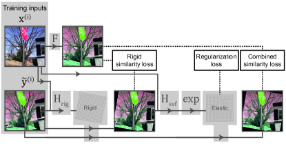
Figure 3: Cross-modality registration architecture. The outputs $y^{(i)}_{\text{reg}}$ and $v^{(i)}_{\text{cross}}$ are forwarded for intra-modality registration. Regularization is applied to both inverse and forward elastic deformation which is not explicitly shown here. The images are from the synthetic ”multimodal” data sets built using COCO [38] data set.

4.3.2 Intra-Modality Registration

The intra-modality registration network receives the triplets

$$(F(x^{(i)}),\overline{y}^{(i)}_{\text{reg}},\exp(-\overline{v}^{(i)}_{\text{cross}})-I)$$

as inputs where $I$ is the identity mapping. The third argument represents displacement field of the inverse elastic deformation with which $y^{(i)}_{\text{reg}}$ has been deformed and allows the network to optimize regularity of the concatenated overall deformation, as we regularize based on that.

Outputs of the cross-modality registration stage are treated as constants by the intra-modality registration losses. By that we prevent the networks from finding any non-desired optima where, e.g., difficult to synthesize regions were made smaller.

Let now the function predicting the stationary velocity field for intra-modality registration be $G_{\text{svf}}$. Then, the predicted intra-modality deformation is

$$d^{(i)}_{\text{intra}}:=\exp(-v^{(i)}_{\text{intra}})$$

where $v^{(i)}_{\text{intra}}:=G_{\text{svf}}(F(x^{(i)}),\overline{y}^{(i)}_{\text{reg}},\exp(-\overline{v}^{(i)}_{\text{cross}})-I)$. Here, we use the negative sign for the velocity field to emphasize that the direction is different from the cross-modality registration. As the training progresses and cross-modality registration and cross-modality image synthesis improve, $d^{(i)}_{\text{intra}}$ should approach the identity mapping.

The loss function for the intra-modality registration is also guiding the cross-modality image synthesis. Hence, we use the deformation equivarince encouraging loss function following the equation (3):

$$\mathcal{L}_{\text{eq-sim}}^{\text{intra}}:=\mathbb{E}_{x,\tilde{y},t}||(d^{*}_{\text{intra}}t^{-1})^{*}F(t^{*}x)-\overline{y}_{\text{reg}}||_{L^{1}}$$ (11)

We also experiment with a setting where the $\mathcal{L}_{\text{sim}}^{\text{intra}}$ is replaced with the default similarity loss following the equation (1). In that case, the loss simply takes the following form:

$$\mathcal{L}_{\text{def-sim}}^{\text{intra}}:=\mathbb{E}_{x,\tilde{y}} ||(d^{*}_{\text{intra}}F(x)-\overline{y}_{\text{reg}}||_{L^{1}}.$$ (12)

For regularization, we use the concatenated overall elastic deformation again in both directions:

$$\mathcal{L}_{\text{reg}}^{\text{intra}}:=\frac{1}{2}\mathbb{E}_{x,\tilde{y}}[ \operatorname{Rig}(\exp(v_{\text{intra}})^{*}\exp(\overline{v}_{\text{cross}}))$$ (13)

$$+ \operatorname{Rig}(\exp(-\overline{v}_{\text{cross}})^{*}\exp(-v_{\text{intra}}))]$$

Using the concatenated overall deformation is logical, as that is the deformation we are actually trying to learn and hence regularize.

Having the separate intra-modality registration network in addition to the cross-modality registration allows the prediction from the image synthesis network to directly affect the predicted deformation. As a result the cross-modality image synthesis network is efficiently optimized for generating predictions with lowest deformation regularization loss, which can be seen as a meaningful selection criteria among all the possible geometry preserving versions of the synthesized image.

4.4 Masking

Throughout the architecture, images are resampled by deformations, but the sampled locations might be outside the image. We connect each image with a mask that can initially represent invalid regions in the image. Each time an image is resampled, the mask is updated with the regions resampled from outside the image. In similarity losses, we then compare images only within intersections of the masks. Masks contain discrete values and no gradients flow through the masks during the backward-pass, preventing the optimization of the masks themselves. The same procedure is done also for the deformations as they are also resampled by other deformations.

Invalid region masks are also fed for the registration networks since for invalid regions only the regularization should affect the generated deformation.

Additionally, the masks of the registered targets and the predictions registered to the registered targets might be systematically different, which the discriminator could use for separating the images. We mitigate for that by multiplying each image fed to the discriminator by the intersection of the masks of the images compared.

4.5 Overall Loss Function

The overall loss function can be written as

$$\mathcal{L} :=\overbrace{\mathcal{L}_{\text{rig-sim}}^{\text{cross}}}^{H_{\text{rig}}}+\overbrace{\mathcal{L}_{\text{sim}}^{\text{cross}}+\lambda\mathcal{L}_{\text{reg}}^{\text{cross}}}^{H_{\text{svf}}}$$ (14)

$$+\underbrace{\mathcal{L}_{\text{sim}}^{\text{intra}}+\lambda\mathcal{L}_{\text{reg}}^{\text{intra}}+\gamma\mathcal{L}_{\text{com}}+\delta\overbrace{\mathcal{L}_{\text{eq-adv}}}^{D}}_{G_{\text{svf}},F}$$

where $\mathcal{L}_{\text{sim}}^{\text{intra}}$ is either $\mathcal{L}_{\text{eq-sim}}^{\text{intra}}$ or $\mathcal{L}_{\text{def-sim}}^{\text{intra}}$, and $\lambda,\gamma,\delta\in\mathbb{R}$ are loss function weights. Each loss component affects only the weights of the sub-networks written in the curly braces. Note that $D$ is trained to maximize the loss whereas the other networks are trained to minimize it. We use two optimizers, one for discriminator, and one for all the other components. This is different to the works by Arar et al. [1] and Kong et al. [32] which use a separate optimizer for the registration network.

Actual values used for the loss function weights are given in the supplementary materials.

5 Experiments

To evaluate our method, we conduct experiments on four diverse data sets of which two are real world medical imaging data sets, one is a semi-synthetic data set, and one is a synthetically constructed ”multi-modal” data set. We perform an ablation study of the losses proposed and compare the method against multiple baselines. Additionally we evaluate on two data sets the performance when using different distributions of affine transformations with the commutation loss. The aim of the experiments is to establish to a reasonable extent:

1. The performance of our method against earlier cross-modality image synthesis methods which are trainable on non-aligned data.

2. The performance of our method against the standard pipeline where the image pairs are registered before training, assuming that no significant manual effort is put into registering the images.

3. Which types of affine transformations are the most suitable for the equivariance encouraging losses and whether the choice has a large effect on the performance.

On the two real world data sets we use clinically relevant metrics for establishing the best performance.

5.1 Ablation Study

We will use the following naming conventions to reflect loss terms to be included in different experimental configurations:

• EqSim: The equivariance similarity loss from Equation (11) was included.

• DefSim: The default similarity loss from Equation (12) was included.

• Com: The commutation loss from Equation (4) was included.

• EqAdv: The equivariance adversarial loss from Equation (7) was included.

• DefUncondAdv: The default unconditional adversarial loss from pix2pix [22] defined directly between unmodified predictions and targets was included.

• NoReg: Only the cross-modality image synthesis component $F$ with $L^{1}$ similarity loss directly between predictions and unmodified training targets was included.

• Aug: Traditional data augmentation was used for each training input using the same distribution of deformations as what would have been used for the equivariance similarity loss, the commutation loss, and the equivariance adversarial loss.

The cross-modality registration related similarity loss and both of the regularization losses were used in all the trainings except with NoReg setup.

In Section 4 three variants of our developed method were proposed: EqSim, DefSim + Com, and EqSim + Com. Optionally, EqAdv can be combined with any of them. Training with any of the variants should result in a stable convergence and the experiments aim at measuring their relative performance.

Table 1: Deformation parameters for synthetic data sets

	Rigid		Elastic
	Translation	Rotation	$\mu$	$\sigma$	$m$
LR	U($-15$, $15$)	U($-15^{\circ}$, $15^{\circ}$)	U($0$, $400$)	U($40$, $120$)	U($-20$, $20$)
SR	U($-1.5$, $1.5$)	U($-1.5^{\circ}$, $1.5^{\circ}$)	U($0$, $400$)	U($40$, $120$)	U($-2.0$, $2.0$)
LC	($10$, $-10$)	$10^{\circ}$	($120$, $280$)	($60$, $80$)	($20$, $-20$)
SC	($1$, $-1$)	$-1^{\circ}$	($120$, $280$)	($60$, $80$)	($2$, $-2$)
$U$ refers to the uniform distribution independent for each dimension.
All the values except the rotations are in pixel coordinates.

5.2 Baselines

We compare the method against four baselines:

• Pix2pix [22], trainable on paired aligned data.

• RegGAN The method proposed by Kong et al. [32], trainable on paired unaligned data. We use the NICEGAN [11] variant which uses $L^{2}$ adversarial loss as it performed the best.

• NeMAR The method proposed by Arar et al. [1], trainable on paired unaligned data, originally suggested for image registration.

• CycleGAN [66], unsupervised method trainable on unpaired data.

We use the official implementations and modify them for our data sets.

For pix2pix and NeMAR we additionally train variants which use the same losses as the official implementations but our components and optimizers. We denote these variants by adding ”our components” in parenthesis after the method name. For details, see Section S.IV of the supplementary materials. Note also that the method DefSim + DefUncondAdv + Aug corresponds to training our architecture with the losses similar to RegGAN, although RegGAN uses a separate optimizer for the registration network.

Our proposed equivariance losses additionally act as data augmentation. To ensure that the reason for our methods performing better is not simply the effect of seeing more data, we augment the inputs for the baseline methods with the same distribution of deformations as is used for the equivariance similarity loss, the commutation loss, and the equivariance adversarial loss.

5.3 Data sets

5.3.1 Synthetic

We performed an ablation study on very simple synthetic ”multimodal” data sets created using images from COCO data set [38] with unmodified images as input images. Target images were generated by circularly swapping the RGB color channels of the input images and by deforming them with simulated deformations. The simulated deformations were generated by a composition of rotation, translation, and an elastic deformation component generated by exponentiation of a stationary velocity field defined by parameters $\mu,\sigma,m\in\mathbb{R}^{n}$ using the formula

$$m_{i}\mathrm{e}^{-\frac{1}{2}\frac{||(x-\mu)||^{2}}{\sigma_{i}^{2}}},$$ (15)

where $x$ is the spatial coordinate and $i\in{1,\dots,n}$ is the dimension ($n=2$ or $3$). Four data set were generated: LR (Large Random), SR (Small Random), LC (Large Constant), and SC (Small Constant). Used deformation parameters are displayed in Table 1. We centrally cropped all the images to resolution $(400,400)$, to avoid the need to extrapolate values from outside the original image when synthetically deforming the images, for details see Section S.V of the supplementary materials. Training, validation, and test sets all contained $4113$ images.

With this data set, all the experiments were conducted without the adversarial loss to study separately the effects of deformation equivariance encouraging losses. The six models trained using each of the data sets are listed in Table 2.

Compositions of the following transformations were used as simulated deformations for the loss functions and data augmentation:

1. Rotations in range ($-15^{\circ}$, $15^{\circ}$)

2. Orthogonal rotations of either $0^{\circ}$, $90^{\circ}$, $180^{\circ}$, or $270^{\circ}$,

3. Random flips over any axis

No model was trained with aligned data as it would be easily learned perfectly in this setup.

5.3.2 Semi-Synthetic Cross-Modality Brain MRI Synthesis

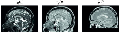
Figure 4: Example images from the semi-synthetic cross-modality MRI synthesis data set. Only one sagittal slide of the 3D volumes is visualized. The training target $\tilde{y}^{(i)}$ has been deformed with a random deformation after which we have cropped it such that the top and bottom edges are straight.

In recent years, a significant amount of research has emerged on applying deep learning to cross-modality brain MRI synthesis. Synthetically generated modalities have many possible down-stream use cases such as segmentation, classification, detection and diagnosis. [62]

We used brain images from Information eXtraction from Images (IXI) data set to generate a semi-synthetic 3D data set for T2 to PD (proton density) synthesis, like in Wang et al. [59]. The main reason for choosing this task was that brain T2 and PD images are initially well aligned and hence provide good ground truths. Most of the images were already in resolution $(1.25\ \text{mm},0.9375\ \text{mm},0.9375\ \text{mm})$, the rest were also resampled to the same resolution. All the images were bias field corrected using N4 bias correction [53] with Advanced Normalization Tools (ANTs) software [5], and normalized based on brain white-matter using the implementation by Reinhold et al. [46] together with the implementation by Iglesias et al. [21] for brain mask extraction by dividing all image values such that the white-matter had mean value of one in each image. We used $192$ images for training, $19$ for validation, and $365$ for testing.

To generate unaligned data set we applied simulated deformations to the target images. The deformations were generated by a composition of rotation, translation, and an elastic deformation component. Translations were sampled from range ($2.0\ \text{mm}$, $10.0\ \text{mm}$), rotations from range ($2.0^{\circ}$, $10.0^{\circ}$), and for elastic deformations we sampled white noise with mean of $10\text{mm}$ and standard deviation of $200\text{mm}$ followed by Gaussian smoothing with standard deviation of $10\text{mm}$. The distribution is intentionally skewed to make the non-desired outcome of over-learning the deformation already in $F$ more attractive. We refer to the unaligned data set as ”unaligned”.

We re-register the synthetically deformed images using popular deformable registration method elastix [30, 49] to compare our method with the standard approach of using registration as a pre-processing step. We refer to this data set as ”registered”.

Additionally we train an oracle model with the original aligned data set and refer to that data set as ”aligned”. For the oracle we use the same generator architecture as for our other methods. Its performance should provide a good upper bound on the performance of our methods.

For our methods we use 3D models and train them by sampling random image patches of size $(64,64,64)$ from the whole training data set. For 2D baseline models we used randomly sampled axial slices. Additionally the inputs were augmented with low-amplitude noise during the training. We also conducted a small experiment on the validation set for determining which type of simulated affine deformations are the most suitable ones for this problem. The experiment included translation, rotation, scaling and shearing. Flipping was not considered since the human anatomy is not symmetric.

5.3.3 Virtual Histopathology Staining

Virtual histopathology staining using deep learning has emerged as an active research topic in recent years, and has been primarily driven by GAN-based methods [6, 47, 45, 31]. However, a majority of the methods require elastic registration of inputs and targets. Our method simplifies the data pre-processing by eliminating the need to elastically register image pairs explicitly.

We used a public data set containing unstained and stained tissue whole slides image (WSI) pairs [27] available at . These are essentially ultra high resolution gigapixel images, and virtually staining the unstained tissue WSIs is a highly non-trivial task. Pre-clinical murine prostate tissue samples were prepared at the University of Eastern Finland, Kuopio. Material used was surplus tissue from previous studies [34, 56] where all animal experimentation and care procedures were carried out in accordance with guidelines and regulations of the national Animal Experiment Board of Finland, and were approved by the board of laboratory animal work of the State Provincial Offices of South Finland (licence number ESAVI/6271/04.10.03/2011). The tissue samples were first scanned without staining. This was followed by hematoxylin and eosin (H&E) staining of the unstained tissue samples, and then the stained samples were scanned again. The samples were scanned using Thunder Imager 3D Tissue slide scanner (Leica Microsystems, Wetzlar, Germany) equipped with DMC2900 camera at 40X magnification level with a pixel size of 0.353µm. Total of 17 WSI pairs were included in the data set each with resolution of approximately $40\text{k}\times 40\text{k}$ from which $9$ were used for training, $1$ for validation, and $7$ for testing.

Inputs and targets were coarsely registered and the alignment seems superficially good. However, upon a closer inspection clear misalignments are present. We additionally registered the images using an open source cross-modality whole slide image registration tool called wsireg. The WSI pairs were registered in two steps, first rigidly for global alignment and then elastically for more granular correspondence between the modalities. We refer to the coarsely registered original data set as ”unaligned” and to the more finely registered data set as ”registered”. No oracle model was trained as we did not have ground truth registrations for this data set.

All of the models were trained by sampling random image patches of size $512\times 512$ from the whole training data set. Additionally the inputs were augmented with low-amplitude noise during the training. On this data set we used the same set of transformations for the equivariance encouraging loss functions as was used in the synthetic experiment. We did not consider scaling or shearing for this data set as the misalignments on a single patch level are essentially rigid. Flipping was included as on the microscopic level the distribution should not be affected by that.

5.3.4 Head MRI to CT synthesis

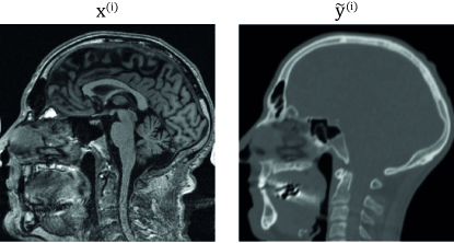
Figure 5: Example training images from the head MRI to CT synthesis data set. Only one sagittal slide of the 3D volumes is visualized. As can be seen, significant misalignments are present at the neck region. ©Copyright CERMEP – Imagerie du vivant, www.cermep.fr and Hospices Civils de Lyon. All rights reserved.

Pseudo CT images are CT-like images generated from MRI images and are mostly used for replacing CT images in external beam radiation therapy (EBRT). Both predicting correct CT-values and geometrical accuracy of the generated images are important. In recent years Deep Learning has emerged as a strong option for pseudo CT generation.[42]

For the experiments we used CERMEP-IDB-MRXFDG data set which is freely available for research use [41]. The data set consists of 37 rigidly registered CT and T1 MRI head scan pairs. We resampled all the images to the MRI-resolution of $160\times 192\times 192$. Pre-processing of the T1 images was similar to the one done for the cross-modality MRI synthesis data set as we applied N4 bias correction [53] using Advanced Normalization Tools (ANTs) software [5] and normalized the brain white-matter to the mean value of one using the implementation by Reinhold et al. [46] together with the implementation by Iglesias et al. [21] for brain mask extraction. We additionally removed any external objects from the CT images using series of morphological operations. While the skull and brain regions are relatively rigid, the image volumes extend to neck region with significant registration mismatches as can be seen in Figure 5. We divided the data set to $20$ cases for training, $5$ for validation, and $12$ for testing.

We refer to the default data set as ”unaligned”. We additionally registered the images elastically using elastix [30, 49] with the hyperparameters by [35] and refer to the data set as ”registered”.

Training setup was very similar to the that of cross-modality MRI synthesis experiment. We used 3D models and trained them by sampling random image patches of size $(64,64,64)$ from the whole training data set and for 2D baseline models we used randomly sampled axial slices. Additionally the inputs were augmented with low-amplitude noise during the training. We still similarly to the cross-modality MRI synthesis experiment conducted an experiment on the validation set for determining which type of simulated affine deformations are the most suitable. Flipping was again not considered since the human anatomy is not symmetric.

5.4 Evaluation

For all the experiments we measure structural similarity index (SSIM) [61], peak-signal-to-noise-ratio (PSNR), and normalized mutual information (NMI) [52]. NMI was applied between inputs and predictions as opposed to inputs and aligned targets as it is used here for measuring the geometric similarity of the predictions to the corresponding inputs. A detailed description of the pixel-wise metrics is given in the supplementary materials.

Additionally we measured the visual appearance of the synthesised images with Fréchet inception distance (FID) metric [19, 48]. While the visual appearance of the images is not usually clinically relevant, we still considered the comparison to be interesting enough to be included. For 3D data sets we computed FID over image slices over all three axes.

Evaluation of the virtual staining and pseudo CT experiments required more careful approaches described in the subsections 5.4.1 and 5.4.2.

5.4.1 Virtual Histopathology Staining Evaluation

We computed the pixel-wise metrics for the virtual staining data set separately for each predicted batch. As no ground truth was available, we registered affinely each stained patch to the corresponding unstained patch using Advanced Normalization Tools (ANTs) software [4, 5]. We did not use directly the registered data set for computing the pixel-wise metrics to avoid the models trained with that data set from benefiting too much by being able to learn the exact registration dynamics (including possible systematic registration errors).

To further evaluate the quality of the virtually stained images, we conducted a comparative analysis of the virtual staining methods for nuclei reproducibility, a downstream validation approach similar to that of Khan et al. [27]. For that analysis we used the images from the registered data set as the ground truth. We employed the nuclei detection method by Valkonen et al. [54] to output nuclei center coordinates in all the WSIs in the test set. First, nuclei were detected for the ground truth followed by nuclei detections in the virtually stained WSI generated by each of compared methods. F1-scores were computed to compare the detected nucleus coordinates of all outputs against those of the ground truth WSIs, using Euclidean distance with a tolerance of 5µm radius derived experimentally and through prior knowledge of typical nucleus dimensions [33, 54]. We defined a true positive as a nucleus center in the virtually stained WSI for which there was a corresponding nucleus center in the ground truth WSI within 5µm radius. A false positive was defined as a nucleus center in the virtually stained WSI for which there was no corresponding nucleus center in the ground truth WSI within the 5µm radius. False negatives were nuclei centers in the ground truth WSI for which there were no matches in the virtually stained WSI within the 5µm radius.

5.4.2 Head MRI to CT Synthesis Evaluation

For pseudo CT evaluation we additionally computed pixel-wise mean absolute error (MAE) and mean error (ME) as they are very widely used for pseudo CT evaluation and better predictors for resulting radiation dose differences than SSIM or PSNR [9]. ME refers to mean signed error over the data set, and can also be negative. ME largely ignores geometrical misalignements between inputs and predictions but on the other hand is robust to registration errors between inputs and targets used for evaluation.

We concluded the registered data set to be inadequate for accurate evaluation and had to develop more nuanced approach for registering the images, although still using the elastix software [30, 49]. We noticed that the registration results improved by registering only part of the image at a time, probably since that way the rigid registration phase was able to account for a larger part of the total deformation. We ended up randomly sampling $20$ masks with radius of $10$ centimeters from each image and registered the image pairs over each of the masks. The evaluation metrics were computed over all the registrations with Gaussian weighting such that the highest weight was given to the coordinates at the center of the registration mask. Additionally we generated bone masks from the images by thresholding and applied the non-rigidity penalty [51] over those regions, improving the bone registration. That allowed us to use lower regularization value for the soft tissue regions improving the registration for those regions as well. We also manually masked out any regions with clear artefacts from the images. With these changes the quality of the registrations improved significantly based on visual evaluation. However, registration errors will always remain which will have to be taken into account in interpreting the results. To mitigate for registrations errors in body outline which end up easily dominating the metrics, we constructed body masks for both the MRI and CT images using morhoplogical operations and ignored in the evaluation the regions where the body masks did not match.

6 Results and Discussion

6.1 Synthetic

Table 2: Results for the synthetic data set experiments

Data set	Model	PSNR	SSIM	NMI
LR	EqSim + Com	36.45	0.9842	1.159
	DefSim + Com	33.95	0.9757	1.155
	EqSim	34.24	0.9781	1.154
	DefSim	-2.705	1.152e-03	1.042
	DefSim + Aug	-3.138	6.303e-04	1.049
	NoReg + Aug	17.39	0.4550	1.079
SR	EqSim + Com	41.68	0.9954	1.165
	DefSim + Com	33.72	0.9737	1.153
	EqSim	35.39	0.9817	1.155
	DefSim	4.369	3.000e-03	1.022
	DefSim + Aug	31.51	0.9559	1.147
	NoReg + Aug	24.44	0.7607	1.123
LC	EqSim + Com	38.78	0.9905	1.162
	DefSim + Com	34.00	0.9745	1.153
	EqSim	35.18	0.9819	1.155
	DefSim	32.74	0.9640	1.149
	DefSim + Aug	-1.537	1.526e-03	1.039
	NoReg + Aug	16.92	0.4617	1.073
SC	EqSim + Com	40.89	0.9919	1.166
	DefSim + Com	34.05	0.9754	1.154
	EqSim	35.89	0.9840	1.157
	DefSim	15.93	0.38.00	1.070
	DefSim + Aug	30.93	0.9501	1.145
	NoReg + Aug	22.54	0.6696	1.114

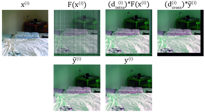
Figure 6: Example failure mode when training without deformation equivariance encouraging losses. The prediction is shifted towards top-left direction and also has a non-desired pattern both of which are compensated by the registration networks. Images are from the synthetic experiment with data set SR and model DefSim.

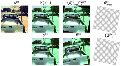
Figure 7: Example prediction from the synthetic experiment with data set LR and model EqSim + Com. The image is from the test set. In addition to the synthesized image, the deformation is accurately reproduced.

Results for the synthetic data set experiment can be seen in Table 2.

The models using the deformation equivariance encouraging losses systematically outperformed the models not using them. Four out of eight trainings with the registration component but without the deformation equivariance encouraging losses did not converge at all to a meaningful optimum. An example prediction of such a training is shown in Figure 6. The performance of the models without the deformation equivariance losses varied a lot and in few cases the performance was even quite good. However, when using either of the deformation equivariance losses the trainings always converged robustly to a meaningful optimum.

Models using both the equivariance similarity loss and the commutation loss performed the best in terms of the similarity metrics. However, the models having only either the equivariance similarity loss or the commutation loss for encouraging deformation equivariance also performed very well and it is questionable whether the differences in performance when using this kind of synthetic data set will be relevant in real world applications.

6.2 Cross-Modality Brain MRI synthesis

Table 3: Results for the cross-modality brain MRI synthesis experiment on the validation set comparing different types of affine transformations for the commutation loss. The experiment was performed using ”DefSim + Com + EqAdv” setup. Translations were sampled from range $[-8\text{mm},8\text{mm}]$, and rotations from range $[-25^{\circ},25^{\circ}]$. Scales and shears were sampled by exponentiating a symmetric matrix with each matrix element being sampled from a zero mean Gaussian distribution with standard deviation of $0.08$. For generating scales non-diagonal values were set to zero.

Transformations	PSNR	SSIM	NMI
Translation	34.33	0.9332	1.111
Translation + rotation	36.43	0.9578	1.122
Translation + rotation + scaling	36.60	0.9621	1.122
Translation + rotation + scaling + shearing	36.90	0.9623	1.125

Table 4: Results for the cross-modality brain MRI synthesis experiment

Data set	Model	PSNR	SSIM	NMI	FID (sag)	FID (cor)	FID (ax)
Non-aligned	EqSim + Com + EqAdv	36.30	0.9564	1.123	5.069	6.283	6.764
	DefSim + Com + EqAdv	36.70	0.9595	1.124	6.302	7.290	7.709
	EqSim + EqAdv	36.73	0.9609	1.119	3.647	5.204	4.981
	DefSim + DefUncondAdv + Aug	26.67	0.6286	1.049	37.94	28.48	23.80
	RegGAN	21.24	0.3037	1.013	48.70	59.52	28.51
	NeMAR	19.98	0.4592	1.036	147.3	170.0	243.1
	NeMAR (our components)	34.83	0.9377	1.107	3.461	4.270	5.243
	CycleGAN	23.32	0.4046	1.027	21.06	19.30	12.59
Registered	Pix2pix	28.96	0.8895	1.095	12.94	16.32	17.80
	Pix2pix (our components)	35.12	0.9386	1.107	10.01	10.95	10.29
Aligned	Pix2pix (our components)	38.14	0.9679	1.111	4.093	5.462	6.514

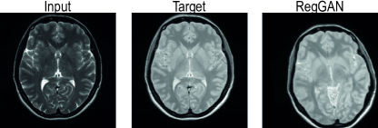
Figure 8: A prediction produced by the RegGAN model in the cross-modality brain MRI synthesis experiment. The model has converged to produce severely misaligned predictions.

Results for the study on a validation set comparing different distributions of affine transformations for equivariance encouraging losses can be seen in Table 3. Based on the study we used combination of all four transformation types in the main experiment for which the results with a test set can be seen in Table 4.

All the three proposed variants of our method performed very well compared to the oracle model trained with aligned data and outperformed all the baselines with statistically significant margin on the voxel-wise metrics. NeMAR which also encourages deformation equivariance coupled with our 3D architecture is the only baseline trained on non-aligned data that came close to our method. RegGAN performed significantly worse and converged to produce severely misaligned predictions as visualized in Figure 8. Pix2pix model trained on the registered data set coupled with our 3D architecture also performed well but was still clearly behind our methods while surpassing all the other models trained on non-aligned data. CycleGAN was also unable to converge to a meaningful optimum due to the large misalignments. While rarely directly relevant in clinical context, our method also performed very well in terms of the FID score.

6.3 Virtual Histopathology Staining

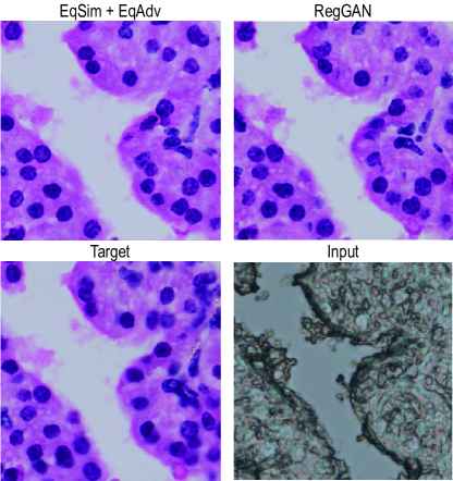
Figure 9: Virtually stained histopathological images with two top-performing models. An area of epithelial cells (pink) with nuclei (blue) is shown.

Results for the virtual histopathology staining experiment can be seen in Table 5.

Nucleus reproduction from unstained brightfield images to virtual stained H&E images is a particularly challenging task, as confirmed by the comparison of nucleus detection results between real and virtual stained images. This is in line with the conclusion from the earlier literature that the locations of all nuclei are simply not available in the unstained input images [27]. Additionally the data is not very uniform which also affects the evaluation metrics as training and test distributions do not match.

In terms of F1-score, which can be considered the main metric, RegGAN performed better than the other methods with statistical significance, and two of our methods were close behind, outperforming other baselines. We suspect that RegGAN benefited from having a generator with 24 times more parameters than our generator (1.1 billion vs. 46 million). Also, with this data set the distributions of the desired predictions $F(x^{(i)})$ and the training targets $\tilde{y}^{(i)}$ are very close to each other, i.e. there are no systematic geometrical differences. In such settings the RegGAN can be expected to perform well. It is left for future work to test our method with a larger generator.

Two of our configurations, EqSim + EqAdv and DefSim + Com + EqAdv, beat both pix2pix variants trained on registered data in terms of F1-score by a statistically significant margin (p-values 0.016 and 0.00020). The result is more significant for the pix2pix model with our components as it was trained with identical architecture to our method. However, it is also noteworthy that the differences in loss function weightings affect the precision-recall balance which again can affect the F1-score, e.g. our training of the vanilla pix2pix had a different loss function balance affecting the precision-recall balance compared to the one trained with our components. For our proposed variants it seems that increasing deformation equivariance increases precision at the cost of recall. The model EqSim + EqAdv which did not have the commutation loss was more inclided to guess nuclei whereas the two other models with the commutation loss placed them in more certain locations. We suspect this is due to the commutation loss more directly promoting deformation equivariance which will require the shape of the nuclei to be known.

NeMAR adversarial training did not converge meaningfully with this data set due to the discriminator being easily able to distinguish between fake and real target images. We suspect that it was due to high frequency components present in this data set which the NeMAR architecture could not replicate for the discrminator due to the issues discussed in Section 4.2. Generator size of the unmodified NeMAR was also way too limited for the task.

Table 5: Results for the virtual histopathology staining experiment. Unmodified NeMAR was not included in the nuclei reproducibility study as it failed to converge to a meaningful optimum.

		Nuclei reproducibility
Data set	Model	F1	Precision	Recall	PSNR	SSIM	NMI	FID
Non-aligned	EqSim + Com + EqAdv	0.7493	0.8514	0.6700	21.33	0.6491	1.020	43.04
	DefSim + Com + EqAdv	0.7597	0.8291	0.7015	21.54	0.6553	1.019	35.00
	EqSim + EqAdv	0.7655	0.8004	0.7340	20.95	0.6358	1.018	21.51
	DefSim + DefUncondAdv + Aug	0.7373	0.8838	0.6328	21.16	0.6409	1.019	42.70
	RegGAN	0.7799	0.7978	0.7647	21.22	0.6475	1.019	12.59
	NeMAR	–	–	–	17.64	0.2791	1.014	333.1
	NeMAR (our components)	0.6846	0.9151	0.5476	20.18	0.5788	1.015	55.35
	CycleGAN	0.5826	0.5712	0.5956	15.94	0.5073	1.039	31.50
	Pix2pix (our components)	0.7051	0.8762	0.5914	20.39	0.6144	1.016	40.82
Registered	Pix2pix	0.7068	0.9195	0.5745	21.69	0.7025	1.023	51.73
	Pix2pix (our components)	0.7514	0.8628	0.6656	20.98	0.6705	1.020	30.28

6.4 Head MRI to CT Synthesis

Table 6: Results for the MRI to CT synthesis experiment on the validation set comparing different types of affine transformations for the commutation loss. The experiment was performed using ”DefSim + Com + EqAdv” setup. Translations were sampled from range $[-8\text{mm},8\text{mm}]$, and rotations from range $[-25^{\circ},25^{\circ}]$. Scales and shears were sampled by exponentiating a symmetric matrix with each matrix element being sampled from a zero mean Gaussian distribution with standard deviation of $0.08$. For generating scales non-diagonal values were set to zero. Only translation and rotation were used for the main experiment as that resulted in the best MAE, although the difference is not very large in comparison to additionally using scaling and shearing. Note that ME largely ignores geometrical misalignements between inputs and predictions.

Transformations	MAE	ME	PSNR	SSIM	NMI
Translation	74.85	-0.2184	26.89	0.8699	1.067
Translation + rotation	68.06	-0.5071	27.50	0.8698	1.075
Translation + rotation + scaling	68.48	6.100	27.46	0.8723	1.077
Translation + rotation + scaling + shearing	68.44	7.488	27.40	0.8727	1.077

Table 7: Results for MRI to CT synthesis experiment. Note that ME largely ignores geometrical misalignements between inputs and predictions.

Data set	Model	MAE	ME	PSNR	SSIM	NMI	FID (sag)	FID (cor)	FID (ax)
Non-aligned	EqSim + Com + EqAdv	67.59	9.091	28.41	0.8733	1.080	19.30	17.78	18.40
	DefSim + Com + EqAdv	65.26	3.677	28.66	0.8794	1.078	22.66	20.33	20.79
	EqSim + EqAdv	66.08	1.752	28.82	0.8846	1.074	22.07	23.08	18.75
	DefSim + DefUncondAdv + Aug	136.8	-0.8551	23.10	0.7431	1.049	49.51	31.95	34.90
	RegGAN	78.58	-5.386	27.39	0.8461	1.069	63.80	49.06	18.47
	NeMAR	83.22	-14.39	27.22	0.8331	1.071	57.13	46.16	36.28
	NeMAR (our components)	67.49	11.60	28.57	0.8810	1.073	16.04	15.14	15.20
	CycleGAN	99.56	8.469	25.73	0.8002	1.061	63.68	54.07	15.77
Registered	Pix2pix	100.9	-3.347	25.82	0.7684	1.064	67.40	65.20	46.79
	Pix2pix (our components)	69.46	-18.31	28.40	0.8787	1.071	28.64	25.11	22.16

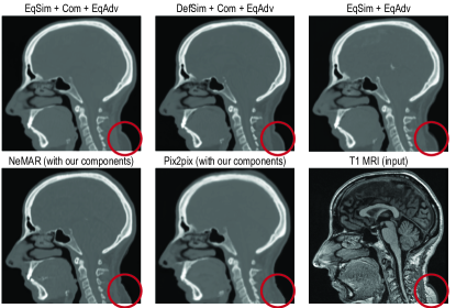
Figure 10: Predictions produced by different variants of our method and the two best performing baselines in the head MRI to CT synthesis experiment. Only our method is capable of generating the body outline at the lower neck region correctly. The region is highlighted with red circles. T1 MRI ©Copyright CERMEP – Imagerie du vivant, www.cermep.fr and Hospices Civils de Lyon. All rights reserved.

Results for the study on validation set comparing different distributions of affine transformations for equivariance encouraging losses can be seen in Table 6. Based on the study we used only translation and rotation in the main experiment for which the results can be seen in Table 7. Note that the differences in metrics when using different affine transformation types are very small and might not be statistically significant.

Our proposed method performed very well in terms of the MAE which can be considered the most important metric for pseudo CT generation due to the strongly linear relationship between CT values and radiation absorption in radiation therapy. DefSim + Com + EqAdv beat all of the baselines with statistically signifcant margin (p-value $0.0024$ compared to NeMAR with our components). EqSim + EqAdv also beat all of the baselines but when using the threshold of $0.05$ in p-value for statistical significance the difference in MAE is narrowly not significant (p-value $0.057$). Encouraging too much equivariance seems to be detrimental for correct CT-value estimation since EqSim + Com + EqAdv performed slightly worse, although still not worse than any of the baselines.

While close to our method metric-wise, under visual inspection the images generated by NeMAR with our components contained more easily visible alignment mistakes than the images generated by our models. Probably the easiest mistake to notice was its inaccuracy in predicting the body outline at neck region, where the data set contains the largest systematic deformation differences. An example of such a case is shown in Figure 10. More subtle mistakes included soft tissue boundaries being placed slightly off. Geometric accuracy of tissue boundaries is important as the pseudo CT images might also be used for positioning at the linear accelerator. The result is in line with the paper introducing NeMAR [1] as in the supplementary materials they conclude that their image-to-image translation network produces geometrically accurate results only when the image synthesis generator model is significantly smaller than the one used here.

FID values have to be looked at with caution since they were calculated with respect to the unaligned data set whose distribution differs from that of the desired unavailable aligned CT images. However, based on visual inspection the NeMAR model with our components indeed produced the most realistic looking texture.

7 Implementation

Implementation of our method in PyTorch framework and all the evaluation implementations can be found at https://github.com/honkamj/non-aligned-i2i. The code base also contains all of the data pre-processing and allows for easily reproducing the results.

8 Conclusions

In this work, we have developed a generic method for training a network for cross-modality image synthesis with paired but misaligned training data by promoting equivariance with respect to simulated deformations. The method is applicable to a wider range of data sets than earlier methods and has the best overall performance accross three different cross-modality image synthesis tasks. On two tasks, cross-modality brain MRI synthesis and head MRI to CT synthesis, the method outperformed all of the baselines, and on the virtual staining task the performance was close to the best performing baseline, even though the baseline had a significantly larger network size. Based on the experiments while the EqSim + Com + EqAdv configuration worked well on the synthetic data, our recommended configurations are EqSim + EqAdv and DefSim + Com + EqAdv as they performed the best on more realistic data sets.

References

- Arar et al. [2020] Arar, M., Ginger, Y., Danon, D., Bermano, A.H., Cohen-Or, D., 2020. Unsupervised multi-modal image registration via geometry preserving image-to-image translation, in: Proceedings of the IEEE/CVF Conference on Computer Vision and Pattern Recognition, pp. 13410–13419.
- Arsigny et al. [2006] Arsigny, V., Commowick, O., Pennec, X., Ayache, N., 2006. A log-euclidean framework for statistics on diffeomorphisms, in: International Conference on Medical Image Computing and Computer-Assisted Intervention, Springer. pp. 924–931.
- Ashburner [2007] Ashburner, J., 2007. A fast diffeomorphic image registration algorithm. Neuroimage 38, 95–113.
- Avants et al. [2008] Avants, B.B., Epstein, C.L., Grossman, M., Gee, J.C., 2008. Symmetric diffeomorphic image registration with cross-correlation: Evaluating automated labeling of elderly and neurodegenerative brain. Medical Image Analysis 12, 26–41.
- Avants et al. [2009] Avants, B.B., Tustison, N., Song, G., et al., 2009. Advanced normalization tools (ants). Insight Journal 2, 1–35.
- Bayramoglu et al. [2017] Bayramoglu, N., Kaakinen, M., Eklund, L., Heikkila, J., 2017. Towards virtual H&E staining of hyperspectral lung histology images using conditional generative adversarial networks, in: Proceedings of the IEEE International Conference on Computer Vision Workshops, pp. 64–71.
- de Bel et al. [2021] de Bel, T., Bokhorst, J.M., van der Laak, J., Litjens, G., 2021. Residual cyclegan for robust domain transformation of histopathological tissue slides. Medical Image Analysis 70, 102004.
- Borovec et al. [2020] Borovec, J., Kybic, J., Arganda-Carreras, I., Sorokin, D.V., Bueno, G., Khvostikov, A.V., Bakas, S., Eric, I., Chang, C., Heldmann, S., et al., 2020. ANHIR: Automatic non-rigid histological image registration challenge. IEEE Transactions on Medical Imaging 39, 3042–3052.
- Boulanger et al. [2021] Boulanger, M., Nunes, J.C., Chourak, H., Largent, A., Tahri, S., Acosta, O., De Crevoisier, R., Lafond, C., Barateau, A., 2021. Deep learning methods to generate synthetic CT from MRI in radiotherapy: A literature review. Physica Medica 89, 265–281.
- Chen et al. [2020a] Chen, L., Liang, X., Shen, C., Jiang, S., Wang, J., 2020a. Synthetic CT generation from CBCT images via deep learning. Medical Physics 47, 1115–1125.
- Chen et al. [2020b] Chen, R., Huang, W., Huang, B., Sun, F., Fang, B., 2020b. Reusing discriminators for encoding: Towards unsupervised image-to-image translation, in: Proceedings of the IEEE/CVF Conference on Computer Vision and Pattern Recognition, pp. 8168–8177.
- Chen et al. [2022] Chen, Z., Wei, J., Li, R., 2022. Unsupervised multi-modal medical image registration via discriminator-free image-to-image translation, in: Raedt, L.D. (Ed.), Proceedings of the Thirty-First International Joint Conference on Artificial Intelligence, IJCAI-22, International Joint Conferences on Artificial Intelligence Organization. pp. 834–840. URL: https://doi.org/10.24963/ijcai.2022/117, doi:10.24963/ijcai.2022/117. main Track.
- Dalca et al. [2018] Dalca, A.V., Balakrishnan, G., Guttag, J., Sabuncu, M.R., 2018. Unsupervised learning for fast probabilistic diffeomorphic registration, in: International Conference on Medical Image Computing and Computer-Assisted Intervention, Springer. pp. 729–738.
- de Bel et al. [2019] de Bel, T., Hermsen, M., Kers, J., van der Laak, J., Litjens, G., 2019. Stain-transforming cycle-consistent generative adversarial networks for improved segmentation of renal histopathology, in: Cardoso, M.J., Feragen, A., Glocker, B., Konukoglu, E., Oguz, I., Unal, G., Vercauteren, T. (Eds.), Proceedings of The 2nd International Conference on Medical Imaging with Deep Learning, PMLR. pp. 151–163. URL: https://proceedings.mlr.press/v102/de-bel19a.html.
- De Vos et al. [2019] De Vos, B.D., Berendsen, F.F., Viergever, M.A., Sokooti, H., Staring, M., Išgum, I., 2019. A deep learning framework for unsupervised affine and deformable image registration. Medical Image Analysis 52, 128–143.
- Fard et al. [2022] Fard, A.S., Reutens, D.C., Vegh, V., 2022. From CNNs to GANs for cross-modality medical image estimation. Computers in Biology and Medicine , 105556.
- Fu et al. [2020] Fu, Y., Lei, Y., Wang, T., Curran, W.J., Liu, T., Yang, X., 2020. Deep learning in medical image registration: a review. Physics in Medicine & Biology 65, 20TR01.
- Hering et al. [2021] Hering, A., Hansen, L., Mok, T.C., Chung, A., Siebert, H., Häger, S., Lange, A., Kuckertz, S., Heldmann, S., Shao, W., et al., 2021. Learn2Reg: Comprehensive multi-task medical image registration challenge, dataset and evaluation in the era of deep learning. arXiv preprint arXiv:2112.04489 .
- Heusel et al. [2017] Heusel, M., Ramsauer, H., Unterthiner, T., Nessler, B., Hochreiter, S., 2017. GANs trained by a two time-scale update rule converge to a local nash equilibrium. Advances in Neural Information Processing Systems 30.
- Hiasa et al. [2018] Hiasa, Y., Otake, Y., Takao, M., Matsuoka, T., Takashima, K., Carass, A., Prince, J.L., Sugano, N., Sato, Y., 2018. Cross-modality image synthesis from unpaired data using CycleGAN, in: International Workshop on Simulation and Synthesis in Medical Imaging, Springer. pp. 31–41.
- Iglesias et al. [2011] Iglesias, J.E., Liu, C.Y., Thompson, P.M., Tu, Z., 2011. Robust brain extraction across datasets and comparison with publicly available methods. IEEE Transactions on Medical Imaging 30, 1617–1634.
- Isola et al. [2017] Isola, P., Zhu, J.Y., Zhou, T., Efros, A.A., 2017. Image-to-image translation with conditional adversarial networks, in: Proceedings of the IEEE Conference on Computer Vision and Pattern Recognition, pp. 1125–1134.
- Jin et al. [2019] Jin, C.B., Kim, H., Liu, M., Jung, W., Joo, S., Park, E., Ahn, Y.S., Han, I.H., Lee, J.I., Cui, X., 2019. Deep CT to MR synthesis using paired and unpaired data. Sensors 19, 2361.
- Joyce et al. [2017] Joyce, T., Chartsias, A., Tsaftaris, S.A., 2017. Robust multi-modal MR image synthesis, in: International Conference on Medical Image Computing and Computer-Assisted Intervention, Springer. pp. 347–355.
- Kaji and Kida [2019] Kaji, S., Kida, S., 2019. Overview of image-to-image translation by use of deep neural networks: denoising, super-resolution, modality conversion, and reconstruction in medical imaging. Radiological Physics and Technology 12, 235–248.
- Kazemifar et al. [2019] Kazemifar, S., McGuire, S., Timmerman, R., Wardak, Z., Nguyen, D., Park, Y., Jiang, S., Owrangi, A., 2019. MRI-only brain radiotherapy: Assessing the dosimetric accuracy of synthetic CT images generated using a deep learning approach. Radiotherapy and Oncology 136, 56–63.
- Khan et al. [2023] Khan, U., Koivukoski, S., Valkonen, M., Latonen, L., Ruusuvuori, P., 2023. The effect of neural network architecture on virtual H&E staining: Systematic assessment of histological feasibility. Machine-Learning .
- Kida et al. [2019] Kida, S., Kaji, S., Nawa, K., Imae, T., Nakamoto, T., Ozaki, S., Ohta, T., Nozawa, Y., Nakagawa, K., 2019. Cone-beam CT to planning CT synthesis using generative adversarial networks. arXiv preprint arXiv:1901.05773 .
- Klages et al. [2020] Klages, P., Benslimane, I., Riyahi, S., Jiang, J., Hunt, M., Deasy, J.O., Veeraraghavan, H., Tyagi, N., 2020. Patch-based generative adversarial neural network models for head and neck MR-only planning. Medical Physics 47, 626–642.
- Klein et al. [2009] Klein, S., Staring, M., Murphy, K., Viergever, M.A., Pluim, J.P., 2009. Elastix: A toolbox for intensity-based medical image registration. IEEE Transactions on Medical Imaging 29, 196–205.
- Koivukoski et al. [2023] Koivukoski, S., Khan, U., Ruusuvuori, P., Latonen, L., 2023. Unstained tissue imaging and virtual hematoxylin and eosin staining of histologic whole slide images. Laboratory Investigation 103, 100070.
- Kong et al. [2021] Kong, L., Lian, C., Huang, D., Li, Z., Hu, Y., Zhou, Q., 2021. Breaking the dilemma of medical image-to-image translation, in: Beygelzimer, A., Dauphin, Y., Liang, P., Vaughan, J.W. (Eds.), Advances in Neural Information Processing Systems. URL: https://openreview.net/forum?id=C0GmZH2RnVR.
- Lammerding [2011] Lammerding, J., 2011. Mechanics of the nucleus. Comprehensive Physiology 1, 783.
- Latonen et al. [2017] Latonen, L., Scaravilli, M., Gillen, A., Hartikainen, S., Zhang, F.P., Ruusuvuori, P., Kujala, P., Poutanen, M., Visakorpi, T., 2017. In vivo expression of miR-32 induces proliferation in prostate epithelium. The American Journal of Pathology 187, 2546–2557.
- Leibfarth et al. [2013] Leibfarth, S., Mönnich, D., Welz, S., Siegel, C., Schwenzer, N., Schmidt, H., Zips, D., Thorwarth, D., 2013. A strategy for multimodal deformable image registration to integrate PET/MR into radiotherapy treatment planning. Acta Oncologica 52, 1353–1359.
- Leynes et al. [2018] Leynes, A.P., Yang, J., Wiesinger, F., Kaushik, S.S., Shanbhag, D.D., Seo, Y., Hope, T.A., Larson, P.E., 2018. Zero-echo-time and Dixon deep pseudo-CT (ZeDD CT): direct generation of pseudo-CT images for pelvic PET/MRI attenuation correction using deep convolutional neural networks with multiparametric MRI. Journal of Nuclear Medicine 59, 852–858.
- Li et al. [2020] Li, Y., Li, W., Xiong, J., Xia, J., Xie, Y., et al., 2020. Comparison of supervised and unsupervised deep learning methods for medical image synthesis between computed tomography and magnetic resonance images. BioMed Research International 2020.
- Lin et al. [2014] Lin, T.Y., Maire, M., Belongie, S., Hays, J., Perona, P., Ramanan, D., Dollár, P., Zitnick, C.L., 2014. Microsoft coco: Common objects in context, in: European Conference on Computer Vision, Springer. pp. 740–755.
- Liu et al. [2021] Liu, S., Zhang, B., Liu, Y., Han, A., Shi, H., Guan, T., He, Y., 2021. Unpaired stain transfer using pathology-consistent constrained generative adversarial networks. IEEE Transactions on Medical Imaging 40, 1977–1989.
- Lu et al. [2021] Lu, J., Öfverstedt, J., Lindblad, J., Sladoje, N., 2021. Is image-to-image translation the panacea for multimodal image registration? A comparative study. arXiv preprint arXiv:2103.16262 .
- Mérida et al. [2021] Mérida, I., Jung, J., Bouvard, S., Le Bars, D., Lancelot, S., Lavenne, F., Bouillot, C., Redouté, J., Hammers, A., Costes, N., 2021. CERMEP-IDB-MRXFDG: A database of 37 normal adult human brain [18F] FDG PET, T1 and FLAIR MRI, and CT images available for research. EJNMMI Research 11, 1–10.
- Owrangi et al. [2018] Owrangi, A.M., Greer, P.B., Glide-Hurst, C.K., 2018. MRI-only treatment planning: Benefits and challenges. Physics in Medicine & Biology 63, 05TR01.
- Peng et al. [2020] Peng, Y., Chen, S., Qin, A., Chen, M., Gao, X., Liu, Y., Miao, J., Gu, H., Zhao, C., Deng, X., et al., 2020. Magnetic resonance-based synthetic computed tomography images generated using generative adversarial networks for nasopharyngeal carcinoma radiotherapy treatment planning. Radiotherapy and Oncology 150, 217–224.
- Pielawski et al. [2020] Pielawski, N., Wetzer, E., Öfverstedt, J., Lu, J., Wählby, C., Lindblad, J., Sladoje, N., 2020. CoMIR: Contrastive multimodal image representation for registration. Advances in Neural Information Processing Systems 33, 18433–18444.
- Rana et al. [2020] Rana, A., Lowe, A., Lithgow, M., Horback, K., Janovitz, T., Da Silva, A., Tsai, H., Shanmugam, V., Bayat, A., Shah, P., 2020. Use of deep learning to develop and analyze computational hematoxylin and eosin staining of prostate core biopsy images for tumor diagnosis. JAMA Network Open 3, e205111–e205111.
- Reinhold et al. [2019] Reinhold, J.C., Dewey, B.E., Carass, A., Prince, J.L., 2019. Evaluating the impact of intensity normalization on MR image synthesis, in: Medical Imaging 2019: Image Processing, International Society for Optics and Photonics. p. 109493H.
- Rivenson et al. [2019] Rivenson, Y., Liu, T., Wei, Z., Zhang, Y., de Haan, K., Ozcan, A., 2019. PhaseStain: the digital staining of label-free quantitative phase microscopy images using deep learning. Light: Science & Applications 8, 1–11.
- Seitzer [2020] Seitzer, M., 2020. pytorch-fid: FID Score for PyTorch. https://github.com/mseitzer/pytorch-fid. Version 0.3.0.
- Shamonin et al. [2014] Shamonin, D.P., Bron, E.E., Lelieveldt, B.P., Smits, M., Klein, S., Staring, M., Initiative, A.D.N., 2014. Fast parallel image registration on CPU and GPU for diagnostic classification of Alzheimer’s disease. Frontiers in Neuroinformatics 7, 50.
- Spadea et al. [2021] Spadea, M.F., Maspero, M., Zaffino, P., Seco, J., 2021. Deep learning based synthetic-CT generation in radiotherapy and PET: A review. Medical Physics 48, 6537–6566.
- Staring et al. [2007] Staring, M., Klein, S., Pluim, J.P., 2007. A rigidity penalty term for nonrigid registration. Medical Physics 34, 4098–4108.
- Studholme et al. [1999] Studholme, C., Hill, D.L., Hawkes, D.J., 1999. An overlap invariant entropy measure of 3D medical image alignment. Pattern Recognition 32, 71–86.
- Tustison et al. [2010] Tustison, N.J., Avants, B.B., Cook, P.A., Zheng, Y., Egan, A., Yushkevich, P.A., Gee, J.C., 2010. N4ITK: improved N3 bias correction. IEEE Transactions on Medical Imaging 29, 1310–1320.
- Valkonen et al. [2020] Valkonen, M., Högnäs, G., Bova, G.S., Ruusuvuori, P., 2020. Generalized fixation invariant nuclei detection through domain adaptation based deep learning. IEEE Journal of Biomedical and Health Informatics 25, 1747–1757.
- Valkonen et al. [2019] Valkonen, M., Isola, J., Ylinen, O., Muhonen, V., Saxlin, A., Tolonen, T., Nykter, M., Ruusuvuori, P., 2019. Cytokeratin-supervised deep learning for automatic recognition of epithelial cells in breast cancers stained for ER, PR, and Ki-67. IEEE Transactions on Medical Imaging 39, 534–542.
- Valkonen et al. [2017] Valkonen, M., Ruusuvuori, P., Kartasalo, K., Nykter, M., Visakorpi, T., Latonen, L., 2017. Analysis of spatial heterogeneity in normal epithelium and preneoplastic alterations in mouse prostate tumor models. Scientific Reports 7, 1–10.
- Wang et al. [2018] Wang, C., Macnaught, G., Papanastasiou, G., MacGillivray, T., Newby, D., 2018. Unsupervised learning for cross-domain medical image synthesis using deformation invariant cycle consistency networks, in: International Workshop on Simulation and Synthesis in Medical Imaging, Springer. pp. 52–60.
- Wang et al. [2019] Wang, C., Papanastasiou, G., Tsaftaris, S., Yang, G., Gray, C., Newby, D., Macnaught, G., MacGillivray, T., 2019. TPSDicyc: Improved deformation invariant cross-domain medical image synthesis, in: International Workshop on Machine Learning for Medical Image Reconstruction, Springer. pp. 245–254.
- Wang et al. [2021a] Wang, C., Yang, G., Papanastasiou, G., Tsaftaris, S.A., Newby, D.E., Gray, C., Macnaught, G., MacGillivray, T.J., 2021a. DiCyc: GAN-based deformation invariant cross-domain information fusion for medical image synthesis. Information Fusion 67, 147–160.
- Wang et al. [2021b] Wang, T., Lei, Y., Fu, Y., Wynne, J.F., Curran, W.J., Liu, T., Yang, X., 2021b. A review on medical imaging synthesis using deep learning and its clinical applications. Journal of Applied Clinical Medical Physics 22, 11–36.
- Wang et al. [2004] Wang, Z., Bovik, A.C., Sheikh, H.R., Simoncelli, E.P., 2004. Image quality assessment: From error visibility to structural similarity. IEEE Transactions on Image Processing 13, 600–612.
- Xie et al. [2022] Xie, G., Wang, J., Huang, Y., Zheng, Y., Zheng, F., Jin, Y., 2022. A survey of cross-modality brain image synthesis. arXiv preprint arXiv:2202.06997 .
- Xu et al. [2019] Xu, Z., Moro, C.F., Bozóky, B., Zhang, Q., 2019. GAN-based virtual re-staining: A promising solution for whole slide image analysis. arXiv preprint arXiv:1901.04059 .
- Yu et al. [2019] Yu, B., Zhou, L., Wang, L., Shi, Y., Fripp, J., Bourgeat, P., 2019. Ea-GANs: Edge-aware generative adversarial networks for cross-modality MR image synthesis. IEEE Transactions on Medical Imaging 38, 1750–1762.
- Zhang et al. [2018] Zhang, Z., Yang, L., Zheng, Y., 2018. Translating and segmenting multimodal medical volumes with cycle-and shape-consistency generative adversarial network, in: Proceedings of the IEEE Conference on Computer Vision and Pattern Recognition, pp. 9242–9251.
- Zhu et al. [2017] Zhu, J.Y., Park, T., Isola, P., Efros, A.A., 2017. Unpaired image-to-image translation using cycle-consistent adversarial networks, in: Proceedings of the IEEE International Conference on Computer Vision, pp. 2223–2232.