Black hole mass estimation using X-ray variability measurements in Seyfert galaxies

Abstract

Aims. Our objective is to critically assess the X-ray flux variability as a tool for measuring the black hole (BH) mass in active galactic nuclei (AGN). We aim to establish a prescription for estimating BH masses based on measurements of the normalised excess variance from X-ray data. We discuss the minimum requirements in terms of the light-curve duration and X-ray signal-to-noise ratio (S/N) to enable a reliable determination that is comparable to what can be derived from the continuum and emission line reverberation studies.

Methods. We used the light curves of local Seyfert from the Nuclear Spectroscopic Telescope Array hard X-ray mission ($\rm NuSTAR$), to compute the normalised excess variance (${\sigma^{2}_{NXV}}$) in the 3-10 and 10-20 keV bands, thus extending the analysis to an energy band higher than 10 keV. The excess variance measurements were then combined with independent BH mass estimates from the literature to establish the ${\rm M}_{\rm BH}$ versus ${\sigma^{2}_{NXV}}$ relation for different samples and weigh its accuracy in terms of the light-curve duration and X-ray S/N.

Results. We find that it is possible to accurately measure the BH mass in AGN using excess variance measurements in the 3-10 and the 10-20 keV bands, however, strong quality requirements should be applied. The minimum necessary S/N and duration of the light curves used to compute the excess variance ought to be $\sim$3 and $\sim 80-100$ ks, respectively. We provide a linear relationship between the normalised excess variance and the black hole mass that can be used to estimate the latter, with an average uncertainty of the order of $0.4-0.25$ dex (depending on the adopted light-curve segment duration). In general, BH mass estimates from 3-10 keV and 10-20 keV band light curves are expected to be similar. The 10–20 keV band is preferred for sources that are heavily absorbed and the 3–10 keV band is preferred for sources that may be dominated by the X–ray reflection component at energies above 10 keV.

1 Introduction

Super-massive black holes (SMBHs) reside in the centre of most (if not all) galaxies and are responsible for their most energetic face, namely, of active galactic nuclei (AGN). According to the current paradigm, the incredibly high luminosity of these objects is powered by the accretion of matter in the vicinity of the SMBHs. As matter spirals inward, copious amounts of energy are released, over a wide range of wavelengths (from radio to gamma rays) due to the conversion of gravitational potential energy into radiation. The emitted power in AGN depends on the black hole (BH) mass and the accretion rate. Their luminosity can reach $10^{15}$ times that of the Sun, while the accretion of matter may significantly contribute to the growth of the BH mass.

Studies have made it clear that SMBHs play a major role in regulating star formation in galaxies and, thus, affect their surroundings. One of the strongest pieces of empirical evidence of the mutual interaction between AGN and its host galaxy is demonstrated by the strong correlation between the mass of SMBHs and the bulge stellar velocity dispersion, $\rm\sigma_{\ast}$, (e.g. Ferrarese & Merritt, 2000; Gebhardt et al., 2000). This relation can be established through the interaction between the energy and radiation generated by accretion and the gas in the host galaxy, known as AGN feedback (e.g. Fabian, 2012).

In order to understand and investigate the role of SMBHs in galaxy formation and evolution processes, we need to monitor the growth of the SMBHs across the cosmic timescale. Therefore, it is not surprising that a lot of effort has been focussed on finding ways of measuring the mass of SMBHs in galaxies – overall, and, in particular, in the case of AGN.

Direct mass measurements of SMBHs are possible with stellar kinematics and gas dynamics, although these methods require good spatial resolution and are presently only feasible for a small number of nearby galaxies. These methods can be used for weak AGN, such as low-luminosity AGNs, LINERs, and Seyfert-2s; this is because for more luminous AGNs, the strong nuclear emission weakens the stellar features in the spectrum.

Based on the assumption that the motion of the gas in the broad line region (BLR) of AGNs is dominated by the gravitational influence of the SMBH, we can use the virial equation $\rm M_{BH}$ = ($\rm fR_{BLR}\Delta V^{2}$ )/G to estimate SMBHs. Here, $\rm R_{BLR}$ is the average radius of the emitting gas in the broad line region, usually determined with reverberation mapping (e.g. Peterson et al., 2004), while the velocity dispersion of the gas ($\rm\Delta V$) is measured from the width of the broad emission lines. The dimensionless factor, f, is referred to as a virial coefficient and encapsulates the unknown geometry and dynamics of the broad line region gas. Its true value for each AGN is unknown and, in most cases, an average value is used, based on the assumption that AGNs follow the ${\rm M}_{\rm BH}$ – $\rm\sigma_{\ast}$ relation observed in quiescent galaxies (e.g. Grier et al., 2013).

Black hole masses can also be inferred indirectly from observable quantities that are correlated with the mass of the SMBHs, such as the velocity dispersion of bulge stars, that is, the value of the ${\rm M}_{\rm BH}$ – $\rm\sigma_{\ast}$ scaling relationship (mentioned above) or the bulge luminosity (e.g. Gültekin et al., 2009).

In this work, we focus on the flux variability of AGN as a means of measuring SMBHs. Stochastic variations of the radiated energy is one of the main observational characteristics of the accretion flows onto compact objects and SMBHs in particular. The origin of these variations is still not well understood and could be related to accretion flow instabilities, a flaring corona, or hot-spots orbiting the central compact object (e.g. Gravity Collaboration et al., 2018, 2020).

Although the AGN flux variability is observed across the entire electromagnetic spectrum, analysing light curves at X-ray wavelengths offers several advantages. Stellar processes emit (very) little X-ray radiation and, therefore, observations at these energies arguably provide the cleanest diagnostic of active SMBHs at the centres of galaxies over a broad redshift range and accretion luminosity baselines (e.g. Brandt & Alexander, 2015). The X-ray photons can also penetrate relatively dense gas clouds and be virtually unaffected, thereby providing a representative sampling of the obscured AGN in the Universe. Therefore, X-ray observations enable flux variation measurements across a broad range of AGN (including low-luminosity and obscured objects) that are challenging or even impossible to perform at other wavebands, where the host galaxy emission is dominant. The proximity of the X-ray emitting region to the active black hole implies the possibility of a direct connection between the X–ray flux variations and the physical properties of the system (e.g. black-hole mass or accretion rate).

Past observations have indicated that such a relation exists in AGN. The X-ray power spectral density (PSD) of AGN has been modelled using a bending power-law with a slope of -1 at low frequencies and then a slope of -2 (e.g. McHardy et al., 2004). Various studies have indicated that the PSD bend frequency may be aptly correlated with BH mass and (potentially) with the bolometric luminosity (e.g. Czerny et al., 2001; McHardy et al., 2006; Körding et al., 2007; González-Martín & Vaughan, 2012). However, it is difficult to estimate the PSD in AGN (and, even more so, detect the bending frequency) as this requires long, high signal-to-noise ratios (S/N) and uninterrupted light curves. Therefore, it is not practical to use the bending-frequency versus BH mass relation to measure the BH mass in AGN.

Using the normalised excess variance, ${\sigma^{2}_{NXV}}$, (e.g. Nandra et al., 1997) as an estimator of the intrinsic ’band-variance’ of the source, a tight anti-correlation between ${\sigma^{2}_{NXV}}$ and ${\rm M}_{\rm BH}$ has also been found in the local universe (e.g. Papadakis, 2004; O’Neill et al., 2005; Zhou et al., 2010; Ponti et al., 2012) as well as the high-redshift universe (e.g. Lanzuisi et al., 2014). In particular, the value of ${\sigma^{2}_{NXV}}$ can be estimated much more easily with the available data sets for many types of AGN, both at low and high redshifts. It is for this reason that most of the SMBH mass measurements in AGN are based on the use of the ${\sigma^{2}_{NXV}}$ vs ${\rm M}_{\rm BH}$ relation (e.g. Ponti et al., 2012).

Our objective is to critically assess the X-ray flux variability as a tool for measuring AGN SMBHs. We used the light curves of local Seyfert from the $\rm NuSTAR$ observatory to compute ${\sigma^{2}_{NXV}}$ in the energy bands 3-10 and 10-20 keV. The use of $\rm NuSTAR$ data has allowed us to extend our analysis to an energy band higher than 10 keV, which may be important for obscured AGN. The excess variance measurements are then combined with independent BH mass estimates from the literature to establish the ${\rm M}_{\rm BH}$ vs ${\sigma^{2}_{NXV}}$ relation in AGN. All studies in the past have focused on the reverse relation (i.e. ${\sigma^{2}_{NXV}}$ vs ${\rm M}_{\rm BH}$) as the main goal was the study of the X–ray variability, while our focus here is the estimation of the BH mass in AGN from the excess variance measurements.

We present a prescription to measure SMBH masses using the excess variance measurements and we discuss, for the first time, the minimum requirements in terms of light-curve duration and X-ray S/N values that enable a reliable determination, similar to those derived from the continuum and emission line reverberation studies or the ${\rm M}_{\rm BH}$ – $\rm\sigma_{\ast}$ relation.

2 The sample

Our sample consists of the Seyfert galaxies detected in the 105-month survey of the Burst Alert Telescope, (BAT; Barthelmy, 2004) on board the Gehrels Swift Gamma-Ray Burst observatory (Gehrels et al., 2004), along with archival observations from the NuSTAR mission (Harrison et al., 2013).

The BAT 105 month catalogue (Oh et al., 2018) contains 379 Seyfert-1s and 448 Seyfert-2s galaxies. There are 161 Seyfert-1s and 253 Seyfert-2s (414 in total) that have been observed by NuSTAR until September 2020, with a duration greater than 10 ks. We found 664 independent, archival NuSTAR observations for these sources. In these NuSTAR observations, a total of 114 are flagged as having been affected by increased solar activity and these have been removed from further analysis. Moreover, we restricted our analysis to the low-redshift regime. This is meant to minimise the inconsistencies on the excess variance estimation when using intervals with a fixed length in the observers frame. Therefore, sources with redshift greater than 0.07 (i.e.  the maximum redshift for the sources in the reverberation sample; see Section 2.1 below for details) are not included in the sample. Our final sample consists of 473 independent observation of 300 local AGN – of which 108 are Seyfert-1s and 192 are Seyfert-2s galaxies.

In order to provide a recipe for the ${\rm M}_{\rm BH}$ estimation, we need to study sources with known BH mass. Thus, we kept sources with BH measurements, which are based either on the so-called reverberation mapping technique or on the use of good-quality, host galaxy velocity dispersion measurements, as we explain below.

2.1 The reverberation sample

Reverberation mapping (e.g. Blandford & McKee, 1982) is one of the most direct ways to obtain BH masses in AGNs. It provides an estimate of the size of the BLR from the lag between the variability in the photo-ionising continuum and the broad emission lines. On this basis, it is possible to infer a virial mass for the SMBH in the central region of the AGN.

We cross-correlated the original sample with the sources included in the AGN BH mass database (Bentz & Katz, 2015) to obtain a sample with BH mass measurements based on reverberation mapping technique (hereafter, the ’rev sample’). We adopt the weighted average of the individual BH mass estimates determined from all the emission lines, assuming that ¡f¿=4.3, as suggested by Grier et al. (2013). The rev sample consists of 26 AGN with 86 NuSTAR observations. The average duration per NuSTAR observation in the rev sample is $\sim 80$ ks. The rev sample log is presented in Table LABEL:rev_sample.

2.2 The velocity dispersion sample

Reverberation mapping data are currently available only for a small number of AGN, but the empirical scaling relation between black hole mass and host-galaxy properties, namely, the ${\rm M}_{\rm BH}$ – $\rm\sigma_{\ast}$ relation (e.g. Grier et al., 2013) offers an alternative way to obtain BH mass estimates. To this end, we used the central velocity dispersion measurements ($\sigma_{\ast}$) presented in the first catalogue of the Swift-BAT AGN Spectroscopic Survey (BASS, Koss et al., 2017). These authors provided measurements of $\sigma_{\ast}$ for many AGN in the 70-month Swift BAT all-sky catalogue. We considered only secure velocity dispersion measurements by selecting the data with spectral fitting quality flag value of 1 or 2. Dual AGN systems, as reported in Koss et al. (2012) are excluded from the analysis. There are 84 sources fulfilling these criteria, with 111 NuSTAR observations.

We also searched the Hyperleda database (Paturel et al. (2003)) to obtain additional central velocity dispersion measurements and increase our sample. We find $\rm\sigma_{\ast}$ measurements for 24 new sources (i.e without $\rm\sigma_{\ast}$ measurements in the BASS survey sample) with 49 NuSTAR observations. Before merging the targets from both the BASS project and the Hyperleda database, we checked whether there are any systematic differences in the velocity dispersion estimates between the two samples. We then identified the common sources, that is, sources with $\rm\sigma_{\ast}$ measurements in both the Hyperleda and the BASS databases and compare the corresponding $\rm\sigma_{\ast}$ values. There are 15 common sources in these samples. Figure  1 shows a plot of $\rm\sigma_{\ast,{\rm Hyperleda}}$ vs $\rm\sigma_{\ast,BASS}$. The plot clearly shows that the BASS and the Hyperleda $\rm\sigma_{\ast}$ measurements are very well correlated. There are no large amplitude or systematic deviations from the one-to-one relation and, therefore, we chose to merge the two samples.

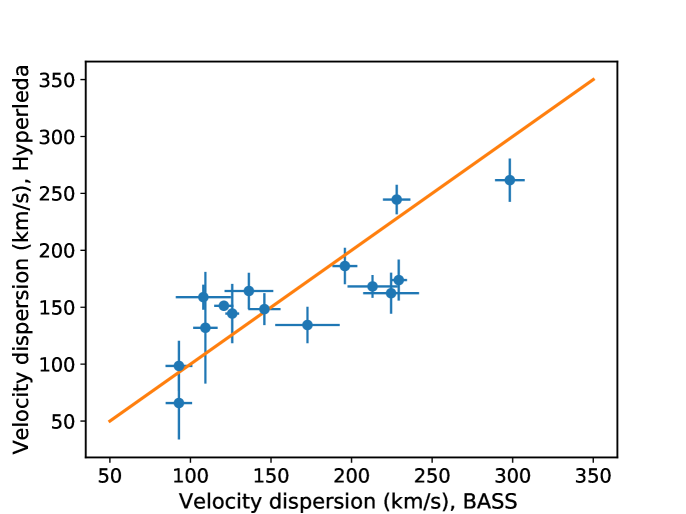
Figure 1: Comparison of the velocity dispersion measurements of the common sources from the Hyperleda database and the BASS catalogue. The error-bars correspond to 1$\sigma$ confidence interval. The solid line show the one-to-one ($y=x$) relation.

In the last step, we cross-correlated the data with Ricci et al. (2017) in order to obtain information on the X-ray column density ($\rm N_{H}$) of each source. We excluded from the sample the Compton thick (CT) sources, namely, the sources with $\rm N_{H}$¿$10^{24}$ $\rm cm^{-2}$. The final velocity dispersion sample (hereafter, the VD sample) is comprised of 84 AGN with reliable measurements of $\rm\sigma_{\ast}$ and 107 NuSTAR observations. The VD sample log is presented in Table LABEL:vd_sample.

For each source in the VD sample, we can estimate the BH mass using the ${\rm M}_{\rm BH}$ – $\rm\sigma_{\ast}$ relation of Woo et al. (2013):

$${\rm logM_{BH}=8.37+5.31\cdot log\left(\frac{\sigma_{\ast}}{200\leavevmode\nobreak\ km\leavevmode\nobreak\ s^{-1}}\right)}.$$ (1)

As shown by Grier et al. (2013), BH mass estimates using Eq. 1 are fully compatible with the masses obtained from the reverberation technique, when assuming a mean virial factor ¡f¿ of 4.3. The mass estimates for the VD sample are also listed in Table LABEL:vd_sample.

2.3 The Compton-thick sample

The sources that have been excluded from the VD sample, due to being CT in nature, make up our CT sample. There are in total 24 CT sources with 53 NuSTAR observations available. These sources are treated separately since their continuum emission, particularly in the 3-10 keV band is severely suppressed, due to heavy absorption, and their spectrum may be dominated by reflected emission (e.g. Baloković et al., 2014). The log of the CT sample is presented in Table LABEL:ct_sample.

3 X-ray data reduction

The observations were processed with the NuSTAR data analysis pipeline (nupipeline) in order to produce cleaned, calibrated event list files. For this standard pipeline processing, we used NuSTAR data analysis software NuSTARDAS v2.0.0 and CALDB version 20170222. From the cleaned event files, we extracted source and background light curves for each of the two NuSTAR focal plane modules (FPMA & FPMB) using the nuproducts script. We adopted a source radius of 60 arcsec for the source light curve extraction, for both FPMA & FPMB observations and applied the live-time, point spread function (PSF), and vignetting corrections. The background light curves are extracted from a four times larger (120 arcsec radius) source-free region of the image at an off-axis angle similar to the source position. We extracted light curves in the 3–10 and 10–20 keV bands, using a bin size of 250 s.

The light curves obtained for the FMPA and FMPB modules were first background subtracted and then summed using the LCMATH tool within FTOOLS. For the subtraction of the background from the source light curves, the proper scaling factors, accounting for the differences in extraction radius for the source and background light curves, have been taken into account. The combined error in the count rate during subtraction or addition of the light curves is always calculated as: $err=\sqrt{err1^{2}+err2^{2},}$ where err1 and err2 are the uncertainties in the count rate in each light curve bin obtained during the NuSTAR data reduction process.

4 The normalised excess variance

To measure the variability power of the sources in our sample we compute the normalised excess variance (e.g. Nandra et al., 1997) using:

$${\rm\sigma_{NXV}^{2}=\frac{1}{N\mu^{2}}\sum_{i=1}^{N}\left(X_{i}-\mu)^{2}-\sigma_{i}^{2}\right),}$$ (2)

where $N$ is the number of bins in the light curve, $\rm X_{i}$ and $\rm\sigma_{i}$ are the count rates and their uncertainties, respectively, and $\mu$ is the unweighted mean count rate.

The $\sigma_{NXV}^{2}$ has been measured using light curve segments with a duration of $\rm\Delta t=10$, 20, 40, and 80 ks. When more than one valid segments are available for a source (for a given timescale, $\rm\Delta t$), we compute the mean of the individual excess variances. This approach should reduce the uncertainty due to the stochastic nature of the X-ray variations (see e.g. Allevato et al., 2013). Following Ponti et al. (2012), all time bins in the light curve segments with fractional exposure lower than 0.35 have been excluded. We note that due to the restriction of our analysis in the local universe (the median redshift of the sample equals 0.02 and the maximum redshift equals 0.07), the impact of the source redshift in the estimation of $\sigma^{2}_{NXV}$ in fixed length intervals is negligible and it is also very similar for all the samples.

Table 1: Best-fit results for the rev and VD $M_{BH}$ vs $\sigma_{NXV}^{2}$ relations

	3-10 keV				10-20 keV
	Rev		VD		Rev		VD
segment	slope	intercept	slope	intercept	slope	intercept	slope	intercept
10 ks	-0.76$\pm$0.12	6.78$\pm$0.07	0.09 $\pm$0.18	7.95 $\pm$0.13	-0.91 $\pm$0.13	6.71$\pm$0.09	0.33$\pm$0.16	7.96$\pm$0.10
20 ks	-0.91$\pm$0.09	7.01$\pm$0.06	-0.05 $\pm$0.13	7.80 $\pm$0.11	-0.96 $\pm$0.14	6.94$\pm$0.11	0.23$\pm$0.16	7.84$\pm$0.09
40 ks	-0.78$\pm$0.15	7.19$\pm$0.08	-0.40 $\pm$0.15	7.59 $\pm$0.10	-1.16 $\pm$0.15	7.25$\pm$0.09	-0.10$\pm$0.21	7.56$\pm$0.11
80 ks	-0.90$\pm$0.09	7.36$\pm$0.07	-1.00 $\pm$0.05	7.42 $\pm$0.07	-1.13 $\pm$0.13	7.36$\pm$0.08	-0.96$\pm$0.21	7.39$\pm$0.08

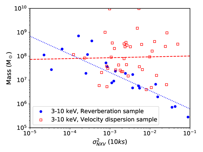
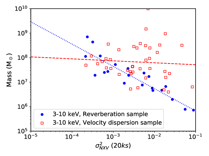
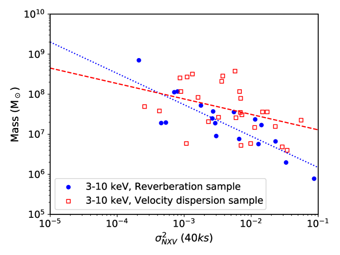
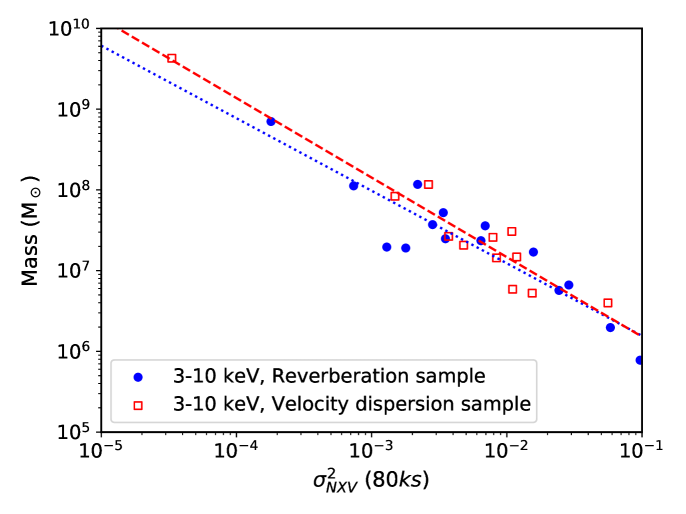
Figure 2: ${\rm M}_{\rm BH}$ vs ${\sigma^{2}_{NXV}}$ in the 3–10 keV band for the rev sample (filled-blue circles) and the VD sample (open-red squares). The dotted blue line and the red dashed line show the best-fit results for the rev and the VD sample, respectively.

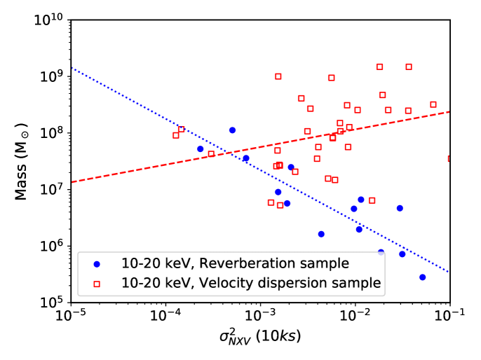
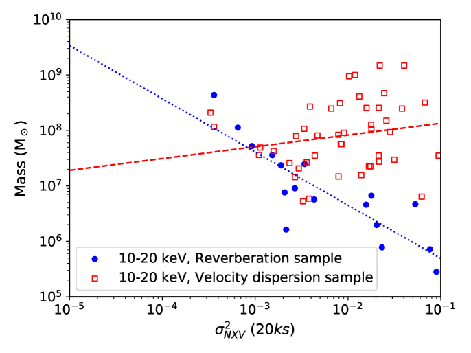
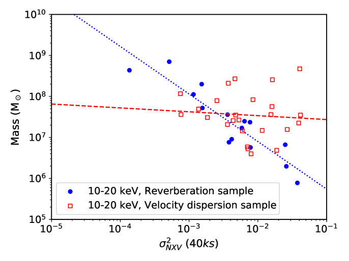
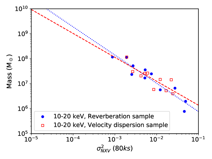
Figure 3: ${\rm M}_{\rm BH}$ vs ${\sigma^{2}_{NXV}}$ in the 10–20 keV band for the rev sample (filled-blue circles) and the VD sample (open-red squares). The dotted blue line and the red dashed line show the best-fit results for the rev and the VD sample, respectively.

5 Measuring ${\rm M}_{\rm BH}$ using $\sigma^{2}_{NXV}$

Previous studies have explored the dependence of the normalised excess variance on the BH mass, ultimately suggesting a linear correlation in the log-log space between the two quantities. We aim to establish a prescription to estimate BH masses given the measurements of the normalised excess variance from X–ray data, therefore, we chose to establish the reverse relation, that is, the relation of ${\rm M}_{\rm BH}$ versus ${\sigma^{2}_{NXV}}$. Our objective is to investigate what are the requirements for the light curves that will be used to compute ${\sigma^{2}_{NXV}}$, so that the resulting BH mass estimates will be as unbiased as possible and of known variance.

Instead of applying, a priory, a certain cut to the S/N value, we simply consider only the sources where the AGN variability is well detected, namely, the computed ${\sigma^{2}_{NXV}}$ is positive (either the mean or a single value, if there is only one light curve segment available). In this way, observations where the S/N ratio is low or the intrinsic amplitude is weak were excluded from further analysis. Then we carried out a separate study of the ${\rm M}_{\rm BH}$ versus ${\sigma^{2}_{NXV}}$ relation for the rev and VD samples in four timescales ($\rm\Delta t=10$, 20, 40, and 80 ks) and we investigate how the ${\rm M}_{\rm BH}$ versus ${\sigma^{2}_{NXV}}$ relation changes with respect to the total duration of the light curves used to compute ${\sigma^{2}_{NXV}}$. In this way (as we show in the following), we are able to establish the minimum requirements for the light curves (i.e. the necessary number of segments and S/N values) in order to acquire a reliable ${\rm M}_{\rm BH}$ estimate.

5.1 ${\rm M}_{\rm BH}$ – ${\sigma^{2}_{NXV}}$ relation for the rev and VD samples

The four panels of Fig. 2 show the ${\rm M}_{\rm BH}$ vs ${\sigma^{2}_{NXV}}$ plots for the rev and the VD samples (filled-blue circles and open-red squares respectively) in the 3–10 keV band, when using segments with durations of 10, 20, 40 & 80 ks. The four panels of Fig. 3 present the same results in the 10–20 keV band.

A strong anti-correlation between ${\rm M}_{\rm BH}$ and ${\sigma^{2}_{NXV}}$ is observed in all timescales for the rev sample. Smaller BH masses show the largest variability amplitude, as has been observed many times in the past. However, this is not the case for the VD sample, especially at timescales shorter than 40 ks (top panels in both figures).

We fit a straight line to each plot, in log-log scale, of the following form,

$${\rm\log(M_{BH})=\alpha\cdot\log(\sigma_{NXV,0.005}^{2})+\beta,}$$ (3)

to model the observed behaviour. The ${\sigma^{2}_{NXV}}$ values have been normalised to the value of 0.005 in order to minimise the error on the line parameters, $\alpha$ and $\beta$. Since our objective is to predict ${\rm M}_{\rm BH}$ from ${\sigma^{2}_{NXV}}$ we used the ordinary least-squares regression of Y on X, OLS(Y—X), where Y is the variable to be predicted (i.e.  $\rm M_{BH}$) and X is the measured variable ($\rm\sigma_{NXV}^{2}$), following the prescription of Isobe et al. (1990).

Table 1 lists the best-fit results and the corresponding 1$\rm\sigma$ uncertainties to the ${\rm M}_{\rm BH}$–${\sigma^{2}_{NXV}}$ plots, both for the rev and the VD samples, at all timescales, in both bands. The best-fit slope for the rev sample remains roughly constant, within the errors, in both bands, while the intercept constantly increases as we move to higher timescales. This is fully consistent with the expectations, as the variance provides a measure of the (intrinsic) PSD integral from the shortest to the longest sampled timescale. In the case of red-noise PSDs, this integral should increase with increasing segment duration, hence, the positive correlation of the best-fit line normalisation with the segment duration ($\rm\Delta t$).

The VD data points shown in Figs. 2 and 3 and the best-fit results show that the situation is more complicated in the VD sample. There is almost a complete lack of correlation between ${\rm M}_{\rm BH}$ and ${\sigma^{2}_{NXV}}$ on the shortest timescales ($\rm\Delta t=10$ & 20 ks), in both energy bands. The situation improves progressively as we move to longer timescales where the intrinsic variability is higher. A clear and strong anti-correlation between ${\rm M}_{\rm BH}$ and ${\sigma^{2}_{NXV}}$  is present only in the $\rm\Delta t=80$ ks plots. In fact, the best-fit results to the rev and VD plots are remarkably similar in the case of $\rm\Delta t=80$ ks.

The inconsistency of the ${\rm M}_{\rm BH}$ versus ${\sigma^{2}_{NXV}}$ relations between the rev and the VD samples at $\rm\Delta t\lesssim 40$ ks could not be attributed to any differences in the accuracy of the BH mass measurements between the two cases. After all, the rev BH mass measurements are based on relations that are ’forced’ to agree with the $\rm M_{BH}-\sigma_{\ast}$ relation. Therefore, the difference between the ${\rm M}_{\rm BH}$ versus ${\sigma^{2}_{NXV}}$ plots for the rev and VD samples when the light curve segments are short is expected to be related to limitations in accurately measuring the X-ray variability of the sources in the VD sample. In the following section, we quantify this limitation and present a prescription for the use of $\rm\sigma_{NXV}^{2}$ in the BH mass determination.

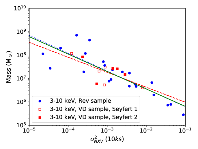
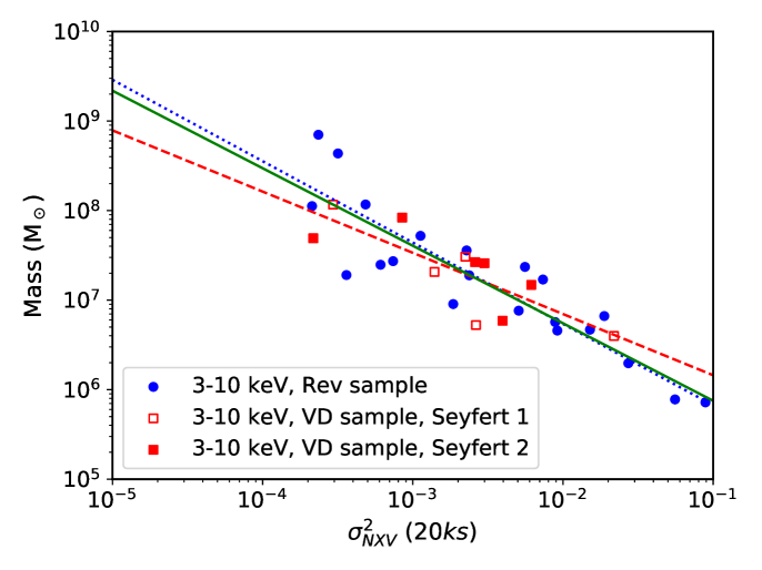
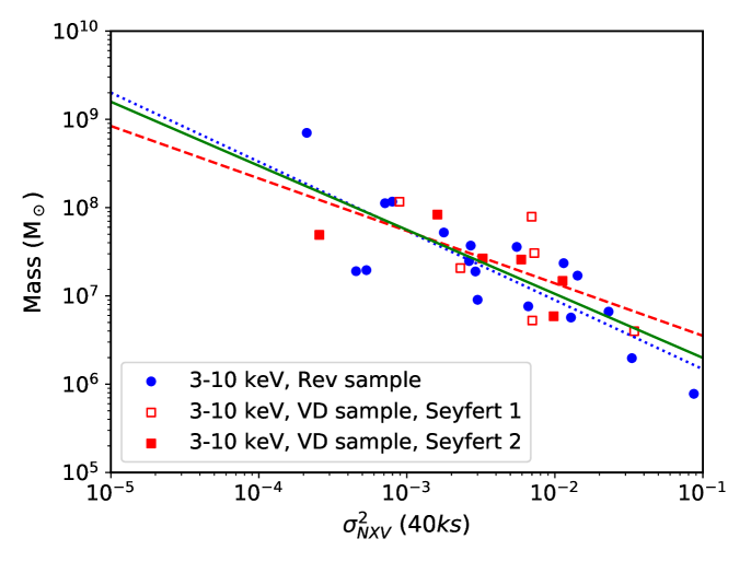
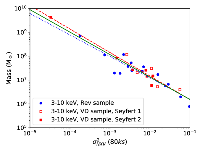
Figure 4: $\rm M_{BH}$ versus $\rm\sigma_{NXV}^{2}$, in the 3–10 keV band, for the final rev and VD sub-samples (chosen as explained in §5.2). Filled-blue circles indicate the rev sample data (Type I AGN) while open-red and filled-red squares indicate Type I and Type II AGN from the VD sample, respectively. The blue-dotted and the red-dashed lines show the best-fit lines to the rev and VD (Type I & Type II) data respectively. The solid green line shows the best fit relation using all the data in each panel.

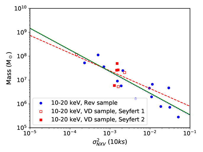
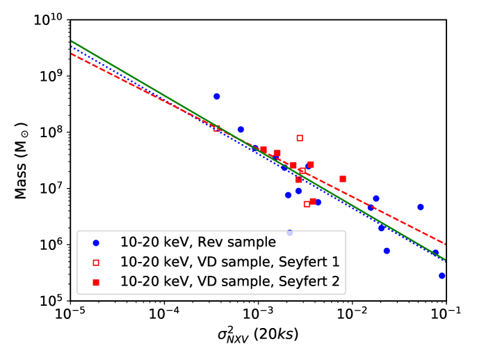
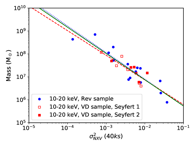
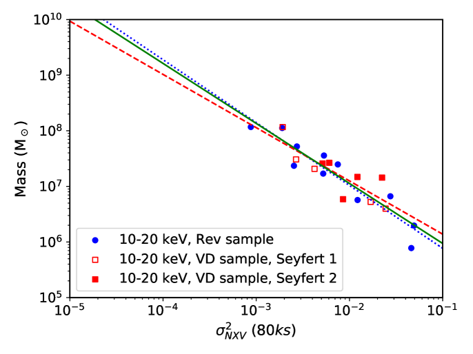
Figure 5: $\rm M_{BH}$ versus $\rm\sigma_{NXV}^{2}$, in the 10–20 keV band, for the final rev and VD sub-samples (chosen as explained in §5.2). Filled-blue circles indicate the rev sample data (Type I AGN) while open-red and filled-red squares indicate Type I and Type II AGN from the VD sample, respectively. The blue-dotted and the red-dashed lines show the best-fit lines to the rev and VD (Type I & Type II) data respectively. The solid green line shows the best fit relation using all the data in each panel.

5.2 Significance of the observation duration

The main difference between the rev and VD samples is the average number of observations per target and their duration. There are, on average, 3.3 observations per source in the rev sample, with a mean duration of 80 ks each. On the contrary, there are only 1.3 observations per target in the VD sample, with a mean duration of 60 ks each. In order to quantify the impact of the available exposure time of a source in the estimation of the $\sigma_{NXV}^{2}$, we performed the following experiment.

For each timescale, we progressively increased the minimum number of light curve segments required in order to keep a target in the sample. Effectively, this leads to smaller and smaller sub-samples, with an increased average duration for the observations. For example, when we request a minimum of at least two time segments of 20 ks for the estimation of ${\sigma^{2}_{NXV}}$, then only sources with one observation of at least $\rm\Delta t=40$ ks or two observations of at least 20 ks each are considered. When, for instance, we increase the minimum number of 20 ks segments to five, then it is only those sources with at least a $\rm\Delta t=100$ ks observation or five observations of 20 ks each are considered. We repeated this exercise, namely, increasing the minimum number of segments for both the rev and the VD samples, until there were less than six sources left in the sample and we stopped.

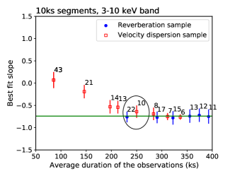
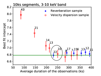
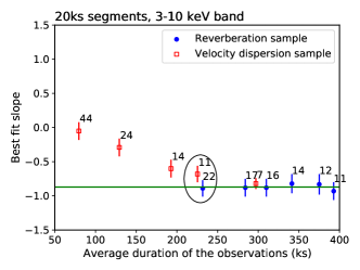
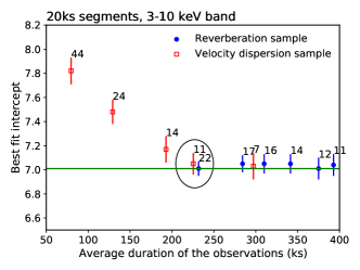
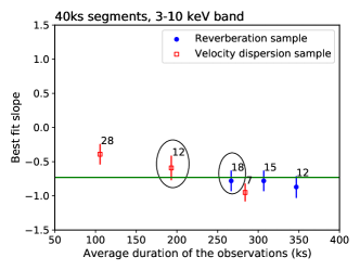
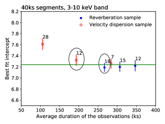
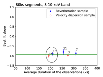
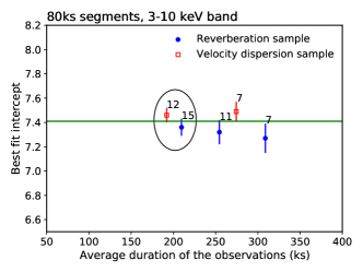
Figure 7: Best-fit slope and intercept in the 3-10 keV band for the rev sub-samples (filled-blue circles) and the VD sub-samples (open-red squares) as a function of the average duration of their sources. The circles indicate the first rev and VD sub-samples (i.e those with a shorter duration) for which the best-fit results are in agreement (within errors). The horizontal lines indicates the best fit value when we fit the combined data from the two sub-samples in agreement (rev and VD).

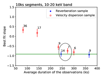
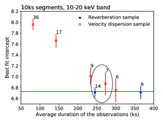
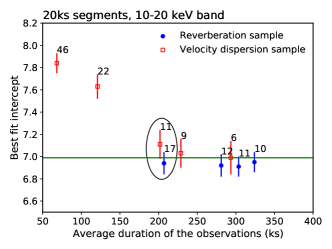
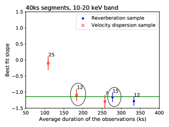
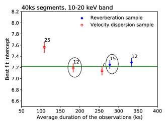
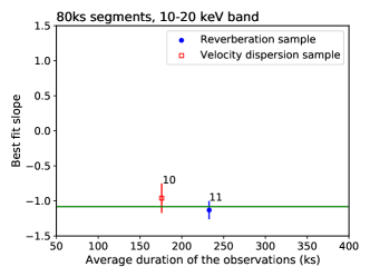
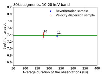
Figure 8: Best-fit slope and intercept in the 10-20 keV band for the rev sub-samples (filled-blue circles) and the VD sub-samples (open-red squares) as a function of the average duration of their sources. The circles indicate the first rev and VD sub-samples (i.e those with a shorter duration) for which the best-fit results are in agreement (within errors). The horizontal lines indicates the best fit value when we fit the combined data from the two sub-samples in agreement (rev and VD).

For each new sub-sample, we again fit a straight line to obtain the best fit slope and intercept of the $\rm M_{BH}$ versus $\sigma_{NXV}^{2}$ relation. Figures 7 and 8 show the resulted best-fit parameters plotted as a function of the average duration of the observations for each sub-sample. The numbers next to each point indicate the number of sources left in each sub-sample after increasing the minimum number of segments.

The best-fit parameters remain roughly constant for the rev sample, irrespective of the number of segments required to compute ${\sigma^{2}_{NXV}}$. An increase in that number does not affect the fitting results. However, this is not the case with the VD sample. The VD sample includes many sources with observations with a significantly shorter average duration than the average duration of the rev sample. The best-fit line parameters change as we increase the number of segments we use to compute ${\sigma^{2}_{NXV}}$. When the average duration of the observations in the VD sub-sample is similar to that of the rev sample, then the best-fit slopes and intercepts become consistent.

We also note, as explained in Isobe et al. (1990), that the best-fit parameter errors may be underestimated for the smaller-sized samples (i.e. for the best-fit parameters determined by fitting the objects with the longest observations). This actually makes the agreement between the rev and VD best-fit parameters even more impressive. It also shows that the systematic bias present in the best-fit parameters when we consider all the VD sample sources is much greater than the statistical uncertainty of the best-fit parameters.

The black circles in Figs.  7 and 8 indicate the first VD and rev sub-samples (i.e. those with a shorter average duration and, therefore, a larger size) for which the best-fit line slope and intercept are consistent (within errors). For all subsequent sub-samples, the best-fit results remain roughly constant.

Our results indicate that an average of $\sim 250$ ks in the duration of the observations per source is necessary for the best-fit results, from both samples, to agree when using 10 ks segments. This number decreases to $\sim 180-200$ ks when the estimation of the $\sigma_{NXV}^{2}$ is based on 40 ks and 80 ks segments. This is probably due to the fact that as the segment duration increases, the intrinsic variance increases as well; therefore, it is easier (for a given S/N) to measure it accurately using slightly shorter average duration of observations. The results are similar for both the 3-10 and the 10-20 keV bands.

6 A prescription for measuring ${\rm M}_{\rm BH}$ in Seyfert galaxies.

Figures 4 and 5 show the ${\rm M}_{\rm BH}$ versus ${\sigma^{2}_{NXV}}$ data for the largest rev and VD samples, where the best-fit line slope and intercept are consistent with each other (see the encircled points in Figs. 7 and 8). The blue-dotted and red-dashed lines indicate these best-fit models to the rev and VD samples, respectively (for the same $\rm\Delta t$ value and energy band).

Our rev sample is comprised of Type I AGN only, since the mass estimation is obtained by the reverberation method. On the other hand, the VD sample, where the mass is estimated using stellar velocity dispersion measurements from high-quality spectra, contains both Type I and Type II AGNs. We note, however, that we do not expect any systematic difference in the ${\rm M}_{\rm BH}$ – ${\sigma^{2}_{NXV}}$ relation for Type I and Type II AGNs. For example, Rani et al. (2017) presented their results on the flux variability on hourly timescales for a large sample of AGN using NuSTAR  and suggested no difference in the variability behaviour between Seyfert 1 and 2 galaxies in all X-ray bands.

To further explore this notion, in Figures 4 and 5, we plot Type I AGN separately from the rev sample (filled-blue circles), Type I AGN from the VD sample (open-red squares), and Type II AGN from the VD sample (filled-red squares). The small number statistics in the individual VD sub-samples does not allow for a separate line fitting analysis. However, the plots clearly show that there are no systematic differences or inconsistencies between the different populations. We therefore chose to combine the samples and fit all the data simultaneously.

The solid green lines in Figs.  4 and 5 show the best-fit lines obtained from the combined (rev+VD) sample. The best-fit results are listed in Table 2 (columns 5 and 6 for the 3–10 keV band, columns 11 and 12 for the 10–20 keV band). We propose for these best fit-line models to be used to measure the BH mass in Seyfert galaxies.

Columns 2 and 8 in the same table present a list of the total number of sources in the combined (rev+VD) sample for each band. The samples are smaller in the 10–20 keV band, mainly because the S/N of the light curves in this band is significantly smaller; hence, there are fewer objects with positive excess variance measurements. Columns 3 and 9 list the average duration of the observations ($\rm\Delta t_{a}$) as well as the average ($N_{A}$) and the minimum ($N_{m}$) number of segments for the the objects in each sample, rounded to the lower integer. Here, $N_{m}$ corresponds to the number of segments of the target with the shortest duration for the observations in the combined sample. Columns 4 and 10 list the average and the minimum S/N of the light curves that we used to compute the excess variance in the combined sample. Lastly, columns 7 and 13 list the average scatter of the points around the best-fit line.

Table 2: Best-fit results of the $\rm M_{BH}$ vs $\rm\sigma_{NXV}^{2}$ relation for the combined rev and VD samples.

Rev+VD (3–10 keV)

Rev+VD(10–20 keV)

$\rm\Delta t^{1}$

N${}_{\rm s}^{2}$

$\rm\Delta t$a/Na/N${}_{\rm m}^{3}$

$\rm S/N_{a/m}^{4}$

${\rm\alpha}^{5}$

$\beta^{6}$

$\sigma_{sc}^{7}$

Nsrc

$\rm\Delta t$a/Na/Nm

$\rm S/N_{a/m}$

${\rm\alpha}$

${\rm\beta}$

$\sigma_{sc}$

10

32

240/24/10

13.6/4.1

-0.74$\pm$0.10

6.78$\pm$0.06

0.42

21

250/25/11

8.5/2.5

-0.91$\pm$0.11

6.73$\pm$0.09

0.35

20

33

230/11/5

13.3/4.2

-0.87$\pm$0.08

7.00$\pm$0.05

0.32

28

210/10/4

8.5/2.5

-0.98$\pm$0.11

6.99$\pm$0.07

0.38

40

30

230/5/2

13.6/4.7

-0.73$\pm$0.13

7.24$\pm$0.06

0.36

27

230/5/2

8.3/2.9

-1.14$\pm$0.12

7.22$\pm$0.06

0.29

80

27

200/2/1

13.7/3.3

-0.94$\pm$0.06

7.41$\pm$0.05

0.26

19

200/2/1

8.9/2.9

-1.08$\pm$0.12

7.38$\pm$0.05

0.23

1 Segment duration in ks.

2 Number of sources in the combined rev+VD samples.

3 Average duration in ks/average number of segments/minimum number of segments

4 Average signal-to-noise ratio /minimum signal-to-noise ratio

5 Best-fit slope, 6 best-fit intercept.7 Average scatter of the points around the best fit.

6.1 The prescription

Based on the results presented in the previous section, we propose the following prescription for the measurement of the BH mass in AGN excess variance measurements.

First, the light curve(s) should be divided into a number of segments, the average ${\sigma^{2}_{NXV}}$ should be computed, and then Equation 3 can be used to derive ${\rm M}_{\rm BH}$, with $\alpha$ and $\beta$ listed in Table 2, depending on the duration of the segment that was chosen and the energy band.

Second, the number of light curve segments that will be used to compute the excess variance should ideally be comparable to the average number of segments listed in Table 2 and (at least) larger than the minimum number of segments listed in the same table. Since the scatter of the points around the best-fit lines decreases with increasing segment duration, we propose the use of the longest possible segment to estimate the BH mass.

Finally, the average S/N of the light curves should be comparable to the average S/N and (at least) greater than the minimum S/N listed in Table 2 (see columns 4 and 10 in Table 2). The smallest S/N values suggest that S/N ratios at least equal to $\sim$3 are necessary to achieve a reliable estimate of the BH mass.

6.2 Compton-thick sources

We used the prescription mentioned above to measure the BH mass of the CT sources. Therefore, we apply the same minimum duration and S/N criteria for the measurement of $\sigma_{NXV}^{2}$ presented above for the sources in the CT sample. Due to the small size of the CT sample and the reduced photon statistics due to the absorption, we were able to measure $\sigma_{NXV}^{2}$ in only four sources when using the 80 ks segments. The number of sources with positive ${\sigma^{2}_{NXV}}$ measurements on shorter timescales is very small (only one or two).

Black cross-marks in Fig. 6 show the ${\rm M}_{\rm BH}$versus $\rm\sigma_{NXV}^{2}$ for the CT sources, in the 3-10 keV (upper panel) and the 10-20 keV band (lower panel) for the 80 ks segments. The solid green line shows the best-fit relation to the combined rev+VD sources. An inspection of Fig. 6 suggests that the $\sigma_{NXV}^{2}$ measurements in the 10-20 keV band are in good agreement with the model. Although the number of the CT sources is small, this result suggests that we could use the variability method to measure the BH mass in CT sources, when we use data in the 10–20 keV band.

On the other hand, the scatter of the BH-mass versus excess variance CT points around the best-fit line in the 3–10 keV is significantly greater. The CT data in the top panel of Fig.  6 may even indicate a lack of correlation between BH mass and variability for the CT sources in the 3–10 keV band. This could be due to the fact that most of the observed flux in the 3–10 keV band may be due to scattered radiation rather than the primary continuum in CT sources, although the limited number of CT measurements do not allow us to reach a firm conclusion in this regard.

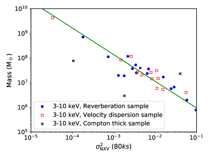
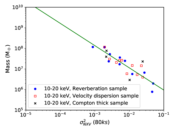
Figure 6: $\rm M_{BH}$ vs $\rm\sigma_{NXV}^{2}$ data for the CT sources in the 3-10 and 10–20 keV bands (upper and lower panel, respectively). $\rm\Delta t=80$ ks, and the solid green line shows the best fit $\rm M_{BH}$-$\rm\sigma_{NXV}^{2}$ relation for the combined rev+VD sample.

7 Application of the proposed prescription

We applied the proposed prescription to obtain BH mass estimates for AGN that are not part of either the rev, VD, or CT samples and that have NuSTAR archival observations which fulfill the minimum number of segments and S/N criteria (as presented in §6.1). There are 22 such sources, which are listed in Table 3 and these constitute our ’prediction’ sample (prd sample, hereafter). The observation log of these sources is presented in Table LABEL:prediction_sample. We followed the same steps as detailed in Sections 3 and 4 to compute $\rm\sigma_{NXV}^{2}$ in the 3-10 and the 10-20 keV bands, using $\rm\rm\Delta t=10$, 20, 40, and 80 ks segments. Then we used the best-fit models listed in Table 2 to estimate the BH mass for each source. Our BH mass predictions are listed in Table 3.

There are two sources (i.e. ESO511-30 and 2MASXJ19301380) where the excess variance is negative, at all timescales and in both energy bands. This is despite the fact that the light curves have a S/N value greater than 3 in both bands and are relatively long, specially in the case of ESO511-30 (BAT ID=719)m where the observation is $\sim$320 ks long. Since all the sources in the rev+VD sample have a positive excess variance measurement and their BH mass is (mostly) smaller than 10⁸M_⊙, we suspect that the mass of the BH in these objects is significantly larger than 10⁸ M_⊙.

Within each energy band, the BH mass estimates from the various light curve segments agree with each other within $1-2\sigma$ (where $\sigma$ is equal to the average scatter of the points around the best-fit line, as listed in Table 2). This is not surprising, as the various light curve segments are all part of the same observations for each source.

The 3–10 keV and the 10–20 keV band BH mass estimates agree within $1-2\sigma$, at all timescales, in all sources, except IRAS09149-6206. In this case, we are able to measure the BH mass using segments with durations of 10, 20, 40m and 80 ks in the 3–10 keV band and the log(${\rm M}_{\rm BH}$) estimates ranging between 7.35 and 7.55. On the other hand, we cannot measure the BH mass using 10 and 20 ks long segments in the 10–20 keV band, because the resulting excess variance is negative. Moreover, the 10–20 keV excess variance using the 40 and 80 ks segments implies a much larger BH mass. The reason for this discrepancy is the fact that a (relatively) large amplitude variation appears in one of the 3–10 keV band light curves, while it is absent in the respective 10–20 keV light curves (see also Walton et al. (2020)).

For two more sources (i.e. Pictor A and HE1143-1810), the excess variance is positive in the 3–10 keV band, but negative in the 10–20 keV band. There are low-amplitude variations in the 3–10 keV band light curves, which do not appear in the 10–20 keV light curves. In both cases, log(${\rm M}_{\rm BH}$) is greater than $\sim 7.6-7.7$. It is possible that the variability detection in the 3–10 keV band only is a statistical effect: due to the high BH mass, it just might happen that the variability is detected only in the 3–10 keV band, where the S/N is greater anyway. Another possibility may be that these sources are dominated by the reflection component at energies above 10 keV; hence, the continuum variations are better sampled at lower energies.

There are also two cases (i.e 3C111 and Mrk 926) where the $\rm\sigma_{NXV}^{2}$ was measured only in the 10-20 keV band. Mrk 926 is the source with the largest BH mass estimate in the prd sample. We believe that the detection of variability in the 10-20 keV and not in the 3–10 keV band is purely statistical in nature. It just happens to measure a positive excess variance in this source at energies above 10 keV; and this is probably the case for 3C111 as well.

Finally, we note that BH mass estimates should always be treated with care. For example, NGC6240, is a galaxy that is known to harbour two active nuclei, each with a mass in excess of $9\times 10^{7}$ M_⊙ (e.g. Kollatschny et al., 2020). Such galaxies are excluded from both the rev and the VD samples. We estimate a log(${\rm M}_{\rm BH}$) of 7.5 - 8.2 (for $\rm\Delta t=40$ ks, in the 10–20 and 3–10 keV bands, respectively), in agreement with the previous estimates. However, we have not explored how the presence of two active nuclei may affect the accuracy of our method.

Table 3: Black hole mass estimates for the prediction sample

BAT ID	Name	Log(M/M⊙)
		80 ks		40 ks		20 ks		10 ks
		3-10keV	10-20keV	3-10keV	10-20keV	3-10keV	10-20keV	3-10keV	10-20keV
163	NGC1194	7.2	6.7	7.07	6.5	–	6.6	–	6.44
184	NGC1365	6.01	6.16	6.39	6.22	6.19	6.27	6.35	6.33
214	3C111	–	7.7	–	7.56	–	7.39	–	7.25
229	HE0436-4717	6.67	6.9	6.72	–	6.94	–	6.87	–
270	PictorA	7.78	–	7.68	–	7.7	–	7.59	–
447	IRAS09149-6206	7.54	8.54	7.35	8.37	7.42	–	7.53	–
472	MCG-5-23-16	7.3	7.34	7.16	7.24	7.03	7.19	6.95	7.05
567	HE1143-1810	–	–	7.63	–	7.83	–	–	–
657	ESO323-77	7.34	7.42	7.55	7.65	7.12	7.17	7.24	7.18
670	MCG-3-34-64	6.56	6.24	6.84	6.39	6.62	6.5	7.06	6.66
692	4U1344-60	7.07	7.05	7.28	7.32	7.19	7.19	7.05	6.98
719	ESO511-30	–	–	–	–	–	–	–	–
750	LEDA3076910	6.61	6.3	6.73	6.31	6.7	6.52	6.69	6.45
837	ESO138-1	–	–	–	–	–	–	–	–
841	NGC6240	–	–	7.99	7.7	8.22	7.52	–	7.96
995	Fairall51	6.7	6.83	6.83	6.77	6.88	6.92	6.8	6.82
1032	ESO141-55	7.14	7.39	7.47	–	7.56	–	7.51	–
1040	2MASXJ19301380	–	–	–	–	–	–	–	–
1111	IGRJ21277+5656	6.85	6.82	6.95	6.83	6.74	6.74	6.62	6.56
1172	MR2251-178	–	–	8.22	8.36	8.1	8.41	7.94	–
1183	Mrk926	–	8.32	–	8.59	–	8.5	–	–
1194	IRAS23226-3843	7.79	8.52	7.61	–	7.83	–	–	–

8 Summary & guidelines

Here, we present a prescription for measuring the mass of the central BH in AGN using excess variance measurements. We emphasise that we did not study the variability versus BH mass relation in AGN, as this has been widely considered in previous studies. Our objective is to select a well-defined sample of sources with available BH mass measurements and then to identify the minimum duration and S/N of the light curves that are necessary for the ${\rm M}_{\rm BH}$versus ${\sigma^{2}_{NXV}}$  relation to be well defined, that is, for the scatter of the points around the best-fit lines to be similar to the average uncertainty of BH mass estimates computed with other methods. If the X-ray variability mechanism is the same for all AGN, we can measure BH mass in any AGN following the prescription we outlined in §6.1, as long as the duration and S/N of the available light curves satisfy the ’quality’ criteria discussed there.

We emphasise that the prescription to measure AGN that we present in this work is only applicable to the case of light curves with a bin size of 250 sec that can be divided in segments of 80, 40, 20, and 10 ks. Such light curves can be obtained from observations taken by NuSTAR and XMM-Newton, as well as from past X–ray observatories, such as Suzaku and ASCA. There are many AGN observations in the RXTE and Swift/XRT archive, however, their mean bin size is significantly larger than 250 sec and, hence, they cannot be used to estimate BH mass using the prescription in Section 6.1. Nevertheless, there are already quite a few AGN whose NuSTAR   and XMM-Newton archival light curves can meet the criteria described in Section 6.1. We already applied our prescription to archival light curves of 22 AGN with NuSTAR  light curves that fulfill the necessary criteria and we computed BH mass estimates for them. In the near future, we plan to search the XMM-Newton archive for AGN with light curves that can satisfy the necessary criteria and estimate their BH mass.

The average scatter of the rev+VD sources around the best-fit line, $\bar{\sigma}_{SC}$, is 0.25, 0.35, and 0.4, for the segments with $\rm\Delta t$=80 ks, 40 and 20 ks, and 10 ks, respectively (these numbers are equal to the mean of $\sigma_{SC,3-10{\rm keV}}$ and $\sigma_{SC,10-20{\rm keV}}$ values, listed in Table 2). On average, the error of log(${\rm M}_{\rm BH}$) should be comparable to $\bar{\sigma}_{SC}$. We stress that $\bar{\sigma}_{SC}$ is not the formal error on the BH mass estimate of an individual source. Instead, it should be considered as representative of the expected standard deviation of these estimates. It is possible to compute the error of log(${\rm M}_{\rm BH}$) for an individual source, but only if the available light curves are long enough (see below).

Our results demonstrate that it is possible to measure the BH mass in AGN using excess variance measurements if the available light curves are long enough and have the necessary S/N values. The resulting BH mass estimates will be as reliable as the estimates which are based on other techniques (e.g. the continuum and emission line reverberation and velocity dispersion measurements). The ’quality’ requirements on the light-curve duration and S/N are quite strong. They are mainly imposed by the statistical properties of ${\sigma^{2}_{NXV}}$. The normalised excess variance is a statistic which follows a highly asymmetric distribution function, with a broad variance (see Allevato et al., 2013). We strongly advise against the use of light curves that do not follow the duration and S/N criteria that we list in Section 6.1. If such light curves are used to compute ${\sigma^{2}_{NXV}}$  and then log(${\rm M}_{\rm BH}$) using the best-fit results listed in Table 2, the resulting estimate may be heavily biased. Due to the ${\sigma^{2}_{NXV}}$  statistical properties, the ${\rm M}_{\rm BH}$  versus ${\sigma^{2}_{NXV}}$ relation may actually depend on the characteristics of the light curves we use (for the same segment duration). For example, the difference between the slope of the best-fit line to the VD data plotted in the top left and bottom right panels in Fig. 2 is 1.09$\pm 0.19$, which is significant at the 5.7$\sigma$ level. This result clearly shows that it will be inappropriate to use the best-fit results listed in Table 2 to compute the BH mass for sources with low-quality light curves.

It may be worth investigating the relation between BH mass and excess variance for shorter light curves or light curves with lower S/N and to establish a prescription for estimating their ${\rm M}_{\rm BH}$  values as well. In this way, BH masses could be measured for many more sources. This aspect, however, is beyond the scope of this work and, in any case, we suspect that the resulting estimates will have significantly larger uncertainties, hence, they may be of limited applicability.

Table 2 lists the best-fit parameters of the lines we fitted to the data of the combined (rev+VD) sample, when the excess variance is computed using light curve segments which are $\rm\Delta t=10$, 20, 40 and 80 ks long (Figs. 4 and 5). We expect that the BH mass estimates should be independent of the segment duration. However, whenever possible, it would be advisable to compute ${\rm M}_{\rm BH}$  using all four different light-curve segment durations to verify that there are no unexpected complications with the observations. Since the average error of the BH estimates should decrease with increasing segment duration, we propose to adopt BH mass estimates based on the longest $\rm\Delta t$.

The accuracy of the BH mass estimate will not increase even if the duration of the light curves is longer than the longest light curves among the sources in the rev+VD sample. This is because the uncertainty on ${\rm M}_{\rm BH}$ mainly depends on the uncertainty of the best-fit line parameters, which should be representative of the typical scatter of the points plotted in Figs 4 and 5. On the other hand, if there are more than 50 segments, with an average S/N ratio greater than 3, then it is possible to compute the error on the mean ${\sigma^{2}_{NXV}}$ (see Allevato et al., 2013). In this case, an error on the BH mass measurement of the individual source can be measured, using the error of the best-fit line parameters (listed in Table 2) and the commonly used rule of error propagation.

The best-fit results and the scatter of the rev and VD points around the best-fit lines are comparable for the 3–10 and the 10–20 keV bands (see Figs.  4 and 5). Black hole mass estimates should be similar when using light curves in both bands to compute the excess variance. Nevertheless, we suggest computing the BH mass in both bands when there are light curves in both bands (i.e. from NuSTAR observations). The 10–20 keV band should be preferred for sources which are heavily absorbed (as our results, from a limited number of CT sources, indicate). On the other hand, the 3–10 keV band should be preferred for sources which may be dominated by the X–ray reflection component at energies above 10 keV.

The ${\rm M}_{\rm BH}$-${\sigma^{2}_{NXV}}$ relations studied here are well calibrated for sources with BH mass between 10${}^{6}-10^{8}$M_⊙. We caution against the use of the proposed method for sources with ${\rm M}_{\rm BH}$$\leq 10^{6}$M_⊙. In this regime, the relation between ${\rm M}_{\rm BH}$ and ${\sigma^{2}_{NXV}}$ could significantly deviate from the linear assumption adopted in this paper. On the other hand, the method we present should be valid for AGN with larger BH masses, although the available data sets for such sources may not be sufficient. The best-fit line in Figs. 4 and 5 show that the normalised excess variance in sources with BH mass larger than 10⁸ M_⊙ should be smaller than $\sim 10^{-3}$, even when $\rm\Delta t=80$ ks (the limit is smaller for shorter segments). This is a small excess variance limit and light curves with the minimum S/N and duration requirements will probably result in a negative ${\sigma^{2}_{NXV}}$. It will be necessary to use light curves with a much higher S/N or many light curve segments in order to measure such a low intrinsic excess variance.

The proposed prescription should be valid both for Type I and Type II objects. Although all AGN in the rev sample are Type I, the VD sample contains a mixture of Type I and Type II sources. Our plots show no difference in the ${\rm M}_{\rm BH}$ – ${\sigma^{2}_{NXV}}$ relation for these two classes and, moreover, the best-fit lines to the rev and VD log(${\rm M}_{\rm BH}$) – ${\sigma^{2}_{NXV}}$  plots are almost identical. Therefore we expect the method to perform equally well for objects in either class.

In this work, we study mainly radio-quiet AGN, although a limited number of objects from the 3C (and one for the 4C) catalogue are included in our sample. Emission from the jet is not supposed to be dominant in the bands we study for any of these sources and we therefore expect the proposed prescription to be valid for these sources as well. In any case, we strongly advise against the use of the proposed prescription to blazars. In this class of sources, in constrast to their radio-quiet counterparts, the X-ray emission could be dominated by radiative processes in the relativistic jet. In agreement to this scenario, Rani et al. (2017) suggested that blazars show much greater X-ray flux variation amplitudes as compared to Seyfert galaxies.

In order to compare or combine BH mass measurements using the prescription presented here with those derived using different methods, it is necessary to take into account (when relevant) that our estimators are normalised to the ${\rm M}_{\rm BH}$ – $\sigma_{\ast}$ relation of Woo et al. (2013). We note that our results are applicable for AGN in the nearby Universe (i.e. sources with z$\leq 0.07$). Our prescription should also be applicable to AGN further away, as long as rest-frame light curves satisfy the necessary quality-criteria. Obviously, the reliability of the BH mass estimates in this case will also depend on the assumption that the AGN variability properties do not change with redshift.

It would be interesting to see if a similar method can be established for the AGN light curves resulting from e-ROSITA sky survey data. The method will have to be calibrated appropriately, as the light curve sampling properties will be entirely different to the light curves that are currently delivered by the pointed observations of XMM-Newton and NuSTAR . It is not certain that it will be possible to measure AGN using variability measurements with the e-ROSITA light curves, but given the large amount of sources that will be identified, it may be worth investigating this possibility.

Appendix A Plots of the best-fit results as function of observation durations

Appendix B Observation logs

Table 4: Log of the rev sample

BAT ID	Name	NuSTAR ObsID	z	Type	Duration	$\rm log(M/M_{\odot})$	Ref.
					(sec)
(1)	(2)	(3)	(4)	(5)	(6)	(7)	(8)
6	Mrk335	60001041005	0.025	Sy1.2	191700	7.23	1, 2, 3, 5, 6, 7, 8, 9
		80201001002			167400
		80001020002			138000
		80502636006			96000
		80502636002			94500
		90602619006			64800
		90602619004			63900
		80502636004			48900
		90602619008			48000
		60001041002			45900
		60001041003			42900
		90602619002			24600
73	Fairall9	60001130002	0.047	Sy1.2	74700	8.29	2, 7, 9, 10, 11
116	Mrk590	90201043002	0.026	Sy1.5	96900	7.57	2, 6, 7, 9
		60160095002			39900
		80402610002			39300
266	Ark120	60001044004	0.032	Sy1.0	132600	8.06	2, 6, 7, 9
310	UGC3374	60201027002	0.020	Sy1.5	184200	7.28	12, 13
458	Mrk110	60201025002	0.035	Sy1.5	387000	7.29	2, 6, 9 14
497	NGC3227	60202002014	0.003	Sy1.5	97800	6.75	2, 9, 13, 15, 16
		60202002002			96000
		60202002008			86400
		60202002010			86100
		60202002004			84000
		80502609004			63600
		80502609002			57000
530	NGC3516	60002042004	0.008	Sy1.2	110100	7.39	2, 9, 13, 15, 16
		60002042002			71400
		60160001002			70500
		60302016012			57900
		60302016010			55500
		60302016004			53400
		60302016006			53100
		60302016002			45600
		60302016008			37800
542	Arp151	60160430002	0.021	Sy1.2	39000	6.67	9, 17, 18, 19, 20
558	NGC3783	60101110004	0.009	Sy1.2	88800	7.37	2, 9, 21, 22, 23, 24
		60101110002			86100
		80202006002			56400
566	UGC6728	60160450002	0.006	Sy1.2	27600	5.85	25, 26
583	Mrk1310	60160465002	0.019	Sy1.5	39300	6.21	9, 17, 18
585	NGC4051	60001050008	0.002	Sy1.5	102900	5.89	2, 9, 12, 13, 27
		60001050006			95400
		60001050003			86100
		60001050002			16800
595	NGC4151	60001111005	0.003	Sy1.5	119700	7.55	2, 7, 9, 13, 15, 28, 29, 30, 31, 32
		60502017004			87000
		60502017006			62700
		60502017002			62100
		60502017008			61800
		60502017012			57000
		60502017010			57000
		60001111002			46200
608	NGC4253	60001048002	0.012	Sy1.5	172800	6.82	9, 17, 18, 33
616	NGC4395	60061322002	0.001	Sy1.0	39000	5.44	34
631	NGC4593	60001149006	0.009	Sy1.0	47700	6.88	2, 9, 35, 36
		60001149004			47700
		60001149010			39900
680	MCG-6-30-15	60001047003	0.007	Sy1.0	261000	6.29	37
		60001047005			57000
		60001047002			46500
686	NGC5273	60061350002	0.003	Sy1.5	39900	6.66	38
697	Mrk279	60160562002	0.030	Sy1.5	37800	7.43	2, 7, 9, 47, 48
717	NGC5548	60002044008	0.017	Sy1.5	98100	7.71	2, 7, 13, 15, 17, 39, 40, 41, 42, 43, 44, 45, 46
		60002044006			97800
		60002044005			97200
		90701601002			73800
774	Mrk290	60061266004	0.029	Sy1.5	41700	7.27	2, 9, 16
984	3C382	60001084002	0.057	Sy1.2	155400	8.84	12, 13
		60202015002			47400
		60202015004			44400
		60202015010			40200
		60202015008			38700
		60202015006			38700
		60061286002			32700
994	3C390.3	60001082003	0.056	Sy1.5	78000	8.63	2, 7, 9, 41, 49, 50, 51, 52, 53, 54
		60001082002			38100
1090	Mrk509	60101043002	0.034	Sy1.2	320400	8.05	2, 6, 7, 9
		60101043004			75000
1182	NGC7469	60101001004	0.016	Sy1.5	45600	6.95	2, 4, 7, 13, 55
		60101001008			45300
		60101001006			45300
		60101001014			45000
		60101001002			41400
		60101001012			39600
		60101001010			39600

Table 4: continued.

Notes: (1) Gehrels SWIFT/BAT catalogue identification number (2) Optical counterpart name (3) NuSTAR observation ID (4) Spectroscopic redshift (5) Optical classification (6) Duration of the NuSTAR observation (7) Logarithm of the source black hole estimate in solar mass units (8) Reference for the stellar velocity dispersion measurement: (1) Grier et al. (2012b), (2) Zu et al. (2011), (3) Grier et al. (2012a), (4) Collier et al. (1998), (5) Hu et al. (2015), (6) Peterson et al. (1998), (7) Peterson et al. (2004), (8) Du et al. (2014), (9) Bentz et al. (2013), (10) Rodríguez-Pascual et al. (1997), (11) Santos-Lleó et al. (1997), (12) Fausnaugh et al. (2017), (13) Dalla Bontà et al. (2020), (14) Kollatschny et al. (2001), (15) De Rosa et al. (2018), (16) Denney et al. (2010), (17) Grier et al. (2013), (18) Bentz et al. (2010), (19) Valenti et al. (2015), (20) Bentz et al. (2008), (21) Bentz et al. (2021), (22) Reichert et al. (1994), (23) Onken & Peterson (2002), (24) Stirpe et al. (1994), (25) Bentz et al. (2016a), (26) Bentz (2021), (27) Denney et al. (2009), (28) Clavel et al. (1990), (29) Metzroth et al. (2006), (30) Ulrich & Horne (1996), (31) Maoz et al. (1991), (32) Bentz et al. (2006), (33) Bentz et al. (2009), (34) Peterson et al. (2005), (35) Barth et al. (2013), (36) Denney et al. (2006), (37) Bentz et al. (2016b), (38) Bentz et al. (2014), (39) De Rosa et al. (2015), (40) Pei et al. (2017), (41) Kovačević et al. (2014), (42) Clavel et al. (1991), (43) Korista et al. (1995), (44) Dietrich et al. (1993), (45) Peterson et al. (2013), (46) Peterson et al. (2002), (47) Maoz et al. (1990), (48) Santos-Lleó et al. (2001), (49) Dietrich et al. (2012), (50) O’Brien et al. (1998), (51) Sergeev et al. (2017), (52) Dietrich et al. (1998), (53) Sergeev et al. (2011), (54) Shapovalova et al. (2010), (55) Peterson et al. (2014)

Table 5: Log of VD sample

BAT ID	Name	NuSTAR ObsID	z	Type	Duration	$\rm Log(M/M_{\odot})$	Ref.	$\rm N_{H}$
					(sec)			$(\rm cm^{-2})$
(1)	(2)	(3)	(4)	(5)	(6)	(7)	(8)	(9)
62	IC1657	60261007002	0.012	Sy2	86100	6.93	1	23.40
		60061008003			23400
63	NGC454E	60061009002	0.012	Sy2	41100	8.41	1	23.30
74	NGC513	60061012002	0.019	Sy2	27600	7.64	1	22.78
77	Mrk359	60402021010	0.017	Sy1.5	100200	6.60	1	20.61
		60402021006			98700
		60402021004			98400
84	NGC612	60061014002	0.030	Sy2	31500	8.98	1	23.97
102	NGC788	60061018002	0.013	Sy2	28800	8.03	1	23.82
157	NGC1142	60368001002	0.028	Sy2	41400	9.29	1	23.76
171	UGC2638	60160148002	0.023	Sy2	44400	7.56	1	22.86
216	NGC1566	80401601002	0.005	Sy1.5	151800	6.72	2	20.00
		60501031006			149400
		60501031004			134400
		80502606002			116700
		80301601002			111000
		60501031002			104700
260	2MASXJ05081967+1721483	60006011002	0.017	Sy1.9	27600	8.49	1	22.33
279	ESO553-43	60160236002	0.027	Sy2	38700	7.84	1	23.30
308	NGC2110	60061061002	0.007	Sy2	33300	9.29	1	22.94
337	VIIZw73	60061067002	0.041	Sy2	30900	7.30	1	23.74
345	2MASXJ06411806+3249313	60061071002	0.047	Sy2	44400	7.92	1	23.12
349	UGC3601	60160278002	0.017	Sy1	42300	8.50	1	21.40
385	UGC3995B	60061352002	0.016	Sy2	43200	7.55	1	23.92
405	UGC4211	60260001002	0.034	Sy2	39300	8.03	1	23.02
416	Fairall272	60061080002	0.021	Sy2	45300	7.95	1	23.53
426	4C+29.30	60061083002	0.064	Sy2	40200	8.71	1	23.80
430	CASG218	60260002002	0.054	Sy2	39001	8.32	1	23.61
439	Mrk18	60061088002	0.011	Sy1.9	36600	7.59	1	23.08
451	IC2461	60061353002	0.007	Sy2	62700	6.68	1	22.78
453	MCG-1-24-12	60061091010	0.019	Sy2	28800	7.63	1	22.81
		60061091006			28500
		60061091012			22200
		60061091002			22200
		60061091004			20100
471	NGC2992	60160371002	0.007	Sy1.9	37800	7.44	1	21.72
474	4C+73.08	60160374002	0.058	Sy2	22500	9.17	1	23.79
480	NGC3081	60561044002	0.008	Sy2	108900	7.17	2	23.91
509	LEDA93974	60061202002	0.020	Sy2	39900	8.41	1	22.60
515	UGC5856	60061359002	0.025	Sy2	44100	6.77	1	22.60
517	UGC5881	60160409002	0.020	Sy2	39000	7.96	1	22.90
519	Mrk417	60061206002	0.032	Sy2	39600	7.96	1	23.90
528	Z291-28	60160420002	0.047	Sy2	28500	8.21	1	23.15
532	Mrk732	60061208002	0.029	Sy1.5	51300	8.41	1	20.00
533	2MASXJ11140245+2023140	60061324002	0.026	Sy2	43200	8.07	1	23.28
548	NGC3718	60301031004	0.003	Sy1.9	167400	9.63	1	21.96
		60301031008			110400
		60301031006			106500
557	HE1136-2304	80002031003	0.027	Sy1.5	127800	7.32	1	21.30
		80002031002			51300
560	NGC3786	60061349002	0.008	Sy1.9	43200	7.46	2	22.36
568	UGC6732	60161452002	0.009	Sy2	40200	8.52	1	22.28
580	IC751	60061217002	0.031	Sy2	21600	8.50	1	23.88
584	LEDA38038	60061219002	0.028	Sy2	39600	7.75	1	22.46
600	Z187-22	60160481002	0.024	Sy2	39000	7.47	1	23.74
605	Was49b	60061335002	0.063	Sy1	38100	8.18	1	23.41
609	NGC4258	60101046004	0.001	Sy1.9	195600	7.43	2	23.00
		60101046002			103500
615	NGC4388	60501018002	0.008	Sy2	97200	6.74	2	23.52
		60061228002			38400
626	NGC4507	60102051004	0.011	Sy1.9	68700	7.69	2	23.95
		60102051008			57300
629	ESO506-27	60469006002	0.025	Sy2	39300	8.98	1	23.95
630	LEDA170194	60061232002	0.036	Sy2	39900	7.97	1	22.76
653	NGC4941	60061236002	0.004	Sy2	39600	6.60	1	23.91
654	NGC4939	60002036002	0.010	Sy2	42000	7.19	1	23.29
659	NGC4992	60061239002	0.025	Sy2	43500	8.43	1	23.69
669	LEDA46599	60160536002	0.031	Sy2	38700	8.39	1	22.88
674	ESO509-38	60260010002	0.026	Sy1.9	45600	8.45	1	20.00
678	ESO509-IG066	60061244002	0.034	Sy1.9	39000	7.98	1	22.84
684	NGC5283	60465006002	0.010	Sy2	51600	7.56	2	23.15
685	Mrk268	60061246002	0.039	Sy1.9	39600	8.43	1	23.53
694	IC4329A	60001045002	0.016	Sy1.5	310200	8.66	2	21.52
710	2MASXJ14104482-4228325	60160571002	0.033	Sy2	39900	8.10	1	22.78
712	NGC5506	60501015002	0.006	Sy1.9	121200	8.06	2	22.44
		60501015004			93900
723	NGC5610	60160581002	0.016	Sy2	45300	7.55	1	22.56
733	NGC5674	60061337002	0.024	Sy2	39300	7.35	1	22.84
734	NGC5683	60160589002	0.036	Sy1.2	40200	7.54	2	20.00
754	Mrk1392	60160605002	0.036	Sy1.5	39300	8.39	2	20.00
755	2MASXJ15064412+0351444	60301023002	0.037	Sy2	125400	7.16	1	22.18
		60061261002			39000
757	Mrk1393	60376005002	0.054	Sy1	60300	7.90	1	20.28
		60160607002			44100
766	NGC5899	60061348002	0.008	Sy2	43500	8.58	1	23.03
783	NGC5995	60061267002	0.025	Sy1.9	38400	8.55	1	21.97
804	Z367-9	60061270002	0.027	Sy2	38700	9.98	1	23.02
817	SDSSJ163115.52+235257.4	60260011002	0.059	Sy1	42000	8.67	1	21.70
836	LEDA214543	60061273002	0.032	Sy2	39600	9.99	1	22.58
875	NGC6300	60061277002	0.003	Sy2	28800	6.80	2	23.31
960	MCG+7-37-31	60061283002	0.041	Sy2	21900	7.91	1	22.48
		60061283004			15600
971	CGMW5-03333	60160686002	0.067	Sy1.9	44400	7.75	1	22.43
978	LEDA3097193	60061354002	0.022	Sy2	28800	7.44	1	22.98
		60061354004			16500
981	CGMW5-04382	60061285002	0.019	Sy2	42900	8.25	1	23.18
1009	Fairall189	60160700002	0.028	Sy1	33300	7.96	1	20.00
1027	ESO231-26	60160706002	0.062	Sy2	42000	8.76	1	23.38
1049	2MASXJ19471938+4449425	60061292002	0.053	Sy2	33900	9.00	1	22.84
1051	3C403	60061293002	0.059	Sy2	39300	9.17	1	23.69
1135	NGC7172	60061308002	0.008	Sy2	60000	8.32	1	22.91
1156	ESO533-50	60061312002	0.026	Sy2	42300	7.58	1	23.49
1161	Mrk915	60002060002	0.024	Sy1	103800	7.49	1	20.00
1162	UGC12138	60061343002	0.025	Sy1.5	42000	7.35	2	20.00
1177	UGC12282	60160812002	0.017	Sy1	50400	9.96	1	23.76
1202	UGC12741	60061321002	0.017	Sy2	39600	8.61	1	23.82
1409	NGC4579	60201051002	0.005	Sy1.9	253800	7.94	2	20.50

Table 5: continued.

Table 6: Log of CT sample

BAT ID	Name	NuSTAR ObsID	z	Type	Duration	$\rm log(M/M_{\odot})$	Ref.	$\rm N_{H}$
					(sec)			$\rm(cm^{-2})$
70	MCG+8-3-18	60061010002	0.02	Sy2	58200	8.27	1	24.12
81	ESO244-30	60468001002	0.025	Sy2	59700	7.04	1	24.36
144	NGC1068	60302003004	0.003	Sy1.9	110700	7.88	2	25.00
		60002030002			109200
		60302003008			108600
		60002033004			108300
		60002033002			103800
		60302003002			97800
		60302003006			97200
		60002030004			90900
153	NGC1125	60510001002	0.011	Sy2	64500	6.98	1	24.21
165	NGC1229	60061325002	0.036	Sy2	46500	8.10	1	24.00
245	Z420-15	60061053004	0.029	Sy2	34800	8.15	1	24.08
		60061053002			27300
325	Mrk3	60002048004	0.013	Sy1.9	52200	8.56	1	24.06
		60002048002			51900
		60002048006			51000
		60002048010			46800
		60002048008			46200
		60002049004			42000
		60002049002			40500
		60002049006			40200
		60002049010			39900
		60002049008			37800
362	UGC3752	60061072002	0.015	Sy1.9	45300	6.98	1	24.78
440	NGC2788A	60160344002	0.013	Sy2	40500	8.64	1	24.26
		60469001002			37500
467	UGC5101	60001068004	0.039	Sy1.9	44400	8.20	1	24.28
484	NGC3079	60061097002	0.003	Sy2	40200	8.06	2	24.56
518	NGC3393	60061205002	0.012	Sy2	27900	8.34	2	24.40
590	NGC4102	60160472002	0.002	Sy2	39600	8.69	1	24.14
711	Circinus	60002039002	0.001	Sy2	94200	7.67	2	24.36
		30002038004			74400			24.36
		30002038006			66300
		30002038002			34200
739	NGC5728	60061256002	0.009	Sy1.9	49800	8.33	2	24.14
740	Z164-19	60061327006	0.029	Sy1.9	37200	6.70	1	24.64
828	NGC6232	60061328004	0.014	Sy2	63000	7.08	1	24.35
		60061328002			31200
1127	NGC7130	60261006002	0.016	Sy1.9	81000	7.30	1	24.22
		60061347002			39600
1184	NGC7479	60061316002	0.007	Sy1.9	43500	7.21	1	24.16
1188	NGC7582	60201003002	0.005	Sy2	100500	7.15	2	24.15
		60061318002			38100
		60061318004			27900
1198	NGC7682	60368002002	0.017	Sy2	47100	7.17	2	24.27
		60061319002			43200
1262	NGC1320	60061036004	0.008	Sy2	52200	6.99	2	24.10
		60061036002			26400
1302	NGC2273	60001064002	0.006	Sy2	39600	7.56	2	24.10
1425	NGC5194	60201062003	0.002	Sy2	324000	6.47	2	24.70
		60002038002			28500

Table 6: continued.

Notes: (1) Gehrels SWIFT/BAT catalogue identification number. (2) Optical counterpart name. (3) NuSTAR observation ID. (4) Spectroscopic redshift. (5) Optical Classification. (6) Duration of the NuSTAR observation. (7)Logarithm of the source black hole estimate in solar mass units. (8) Reference for the stellar velocity dispersion measurement: (1) Koss et al. (2017), (2) Paturel et al. (2003)-Hyperleda database. (9) X-ray column density

Table 7: Log of the prediction sample

BAT ID	Name	NuSTAR ObsID	z	Type	Duration
					(sec)
(1)	(2)	(3)	(4)	(5)	(6)
163	NGC1194	60501011002	0.013	Sy2	114900
184	NGC1365	60002046003	0.005	Sy2	75900
		60002046009			132300
		60002046007			146100
214	3C111	60202061002	0.048	Sy1.2	39900
		60202061004			91800
		60202061006			104100
229	HE0436-4717	60160197002	0.053	Sy1	39000
		30001061004			116100
270	PictorA	60101047002	0.035	Sy2	225300
447	IRAS09149-6206	90401630002	0.057	Sy1	162600
		60401020002			214500
472	MCG-5-23-16	60001046006	0.008	Sy1.9	207900
567	HE1143-1810	60302002010	0.032	Sy1.2	42600
		60302002006			45000
657	ESO323-77	60202021004	0.015	Sy1.5	80100
		60202021002			80400
		60202021006			80700
		60202021008			86400
670	MCG-3-34-64	60101020002	0.016	Sy1.9	151200
692	4U1344-60	60201041002	0.012	Sy1.9	163800
719	ESO511-30	60502035006	0.022	Sy1	60300
		60502035002			62100
		60502035004			63000
		60502035010			63300
		60502035008			80400
750	LEDA3076910	60061259002	0.016	Sy1.5	39900
		60401022002			188700
837	ESO138-1	60201040002	0.009	Sy2	91800
		60061274002			91800
841	NGC6240	60102042006	0.024	Sy1.9	45000
		60102042004			51300
		60002040002			59700
995	Fairall51	60402014004	0.014	Sy1.5	59400
		60402014006			63300
		60402014002			118200
1032	ESO141-55	60201042002	0.036	Sy1.2	174300
1040	2MASXJ19301380+3410495	60160713002	0.062	Sy1.5	39600
		60376001002			95100
1111	IGRJ21277+5656	60001110003	0.014	Sy1	50100
		60001110007			75000
		60001110002			89100
		60402008004			132300
		60402008010			133800
		60402008008			137400
		60402008006			142800
1172	MR2251-178	60102025004	0.064	Sy1.2	43500
		60102025008			45600
		60102025002			51600
		90601637002			52800
1183	Mrk926	60201029002	0.046	Sy1.5	213600
1194	IRAS23226-3843	80502607002	0.035	Sy2	118800

Table 7: continued.

Notes: (1) Gehrels SWIFT/BAT catalogue identification number. (2) Optical counterpart name. (3) NuSTAR observation ID. (4) Spectroscopic redshift. (5) Optical Classification. (6) Duration of the NuSTAR observation.