Approximation Algorithms for Capacitated Assignment with Budget Constraints and Applications in Transportation Systems

Abstract

In this article, we propose algorithms to address two critical transportation system problems: the Generalized Real-Time Line Planning Problem (GRLPP) and the Generalized Budgeted Multi-Visit Team Orienteering Problem (GBMTOP). The GRLPP aims to optimize high-capacity line plans for multimodal transportation networks to enhance connectivity between passengers and lines. The GBMTOP focuses on finding optimal routes for a team of heterogeneous vehicles within budget constraints to maximize the reward collected. We present two randomized approximation algorithms for the generalized budgeted multi-assignment problem (GBMAP), which arises when items need to be assigned to bins subject to capacity constraints, budget constraints, and other feasibility constraints. Each item can be assigned to at most a specified number of bins, and the goal is to maximize the total reward. GBMAP serves as the foundation for solving GRLPP and GBMTOP. In addition to these two algorithms, our contributions include the application of our framework to GRLPP and GBMTOP, along with corresponding models, numerical experiments, and improvements on prior work.

1 Introduction

In this article, we develop a framework to address two critical applications in transportation systems that aim to improve the efficiency and effectiveness of transit networks while managing costs. These applications include: (i) identifying the optimal set of smart transit lines to operate, considering the dual objectives of facilitating connections between passengers and high-capacity fixed-route transit lines and managing the budget effectively, which we refer to as the Generalized Real-Time Line Planning Problem (GRLPP), and (ii) finding service paths for an optimal set of multiple heterogeneous vehicles with appropriate modes in a network such that the profit sum of serving the nodes in the paths is maximized, subject to the travel time limit of each vehicle and the budget for dispatching vehicles, which we call the Generalized Budgeted Multi-Visit Team Orienteering Problem (GBMTOP).

The motivation behind this research lies in the need to optimize transportation systems by effectively allocating resources to minimize costs and maximize connectivity and service quality. As urban populations grow and transportation demands increase, it is crucial to design and operate efficient transit networks that can adapt to dynamic environments and provide satisfactory services to passengers while maintaining budget constraints.

Here, we provide a formal definition for GRLPP. For simplicity, we postpone the formal definition of GBMTOP to Section 4.2.

Assume that there are $L$ candidate multimodal high-capacity transit lines and $P$ passengers. Each line $l$ has a utilization cost $c_{l}\in\mathbb{R}^{+}$ and an $n_{l}$-dimensional capacity vector $f_{l}:=(f_{l}^{(1)},f_{l}^{(2)},\ldots,f_{l}^{(n_{l})})\in\mathbb{Z}_{+}^{n_{l}}$ for $l\in[L]$, where $[n]={1,2,\ldots,n}$ for any integer $n$.

Each line $l$ with $n_{l}$ edges has an $n_{l}$-dimensional capacity vector. Each entry of the capacity vector of line $l$ is set to be $C\cdot f_{l}$. Given a line $l\in[L]$, a sub-route on line $l$ is defined as any set of consecutive edges on line $l$. Assume there are $m_{l}$ different subroutes on line $l$. For each passenger $p$ and line $l$, they can be assigned to a subroute on line $l$. Then, they will be assigned to a $0-1$ $n_{l}$-dimensional weight vector. If the $i$-th edge of line $l$ is used when passenger $p$ is matched to line $l$, then the $i$-th entry of its weight vector is set to be $1$, and $0$ otherwise. Let $v_{lp}^{(i)}$ denote the value generated by assigning passenger $p$ to line $l$ in association with the $i$-th sub-route on line $l$ for $i\in[m_{l}]$. Let $S=(S_{1},S_{2},\ldots,S_{m_{l}})$ be an assignment of passengers to line $l$, where $S_{i}$ is the set of passengers assigned to line $l$ in association with the $i$-th sub-route. If $p\in S_{i}$ for some $i\in[m_{l}]$, then we say $p\in S$. We say that $S$ is feasible if the sum of the capacity weight vectors of the assigned passengers does not exceed the capacity vector of the line $l$ entry-wise. For each line $l\in[L]$, we define $I_{l}$ as the family of all non-empty feasible assignments of passengers to $l$, and we assume $\emptyset\notin I_{l}$.

For each passenger $p$ and line $l$, the value generated by assigning passenger $p$ to line $l$ in association with the $i$-th sub-route on line $l$ is denoted by $v_{lp}^{(i)}\geq 0$. The incurred cost is denoted by $c_{lp}^{(i)}\geq 0$, which can be interpreted as the corresponding cost for utilizing on-demand vehicles, for example. The assignment of transit lines and the cost for utilizing lines are subject to a budget constraint of $B\in\mathbb{R}^{+}$. Additionally, we define $c_{lS}:=c_{l}+\sum_{p\in S_{i},i\in[m_{l}]}c^{(i)}_{lp}$, where $S$ is a subset of passengers assigned to line $l$. This denotes the total cost of operating line $l$ with the assigned subset of passengers. Let $k:=\frac{B}{\max_{l\in[L],S\in I_{l}}c_{lS}}$. Without loss of generality, we can then scale $B$ to $k$ and scale $c_{lS}$ to be in $[0,1]$ accordingly.

We need to find a subset of lines to be operated, an assignment of passengers to opened lines, and their subroutes on the line to maximize the welfare of the system, subject to the following conditions:

1. The total cost of the opened lines does not exceed the budget.

2. The assignment of passengers and their subroutes on the opened line $l$ respects the capacity constraints of each edge on line $l$.

3. Each passenger is assigned to at most one line with one subroute.

This optimization problem aims to balance the utilization cost, rewards generated by passenger assignment, and budget constraints in the transportation system, and is referred to as the Generalized Real-Time Line Planning Problem (GRLPP)

In general, we can consider passengers as items and lines as bins, where each item $p$ can be assigned to a bin $l$ at most $\rho$ times for some positive integer $\rho$. Furthermore, we can define a feasible set of items $S$ for bin $l$ subject to some feasible conditions, such as capacity constraints in the case of GRLPP. In this case, we refer to the assignment problem as a generalized budgeted multi-assignment problem (GBMAP). Note that in GBMAP, instead of subroute options, the modes of assignment for items to bins are considered. For example, in GRLPP, the subroutes on a line are the modes of assignment for passengers to the line. This problem arises in various applications, such as scheduling, resource allocation, and transportation planning, and can serve as the foundation for solving GRLPP and GBMTOP.

Structure of the paper: The remainder of this paper is organized as follows. In Section 2, we review related work and outline the contributions of our research. In Section 3, we present the two algorithms we have developed and analyze their theoretical properties. Finally, in Section 4, we illustrate the application of our framework to solve the GRLPP and GBMTOP problems.

2 Related Work and Contributions

The GBMAP is a variant of separable assignment problem (SAP). In SAP, there are $L$ bins and $P$ items. For each item $p$ and bin $l$, there is a reward $v_{lp}$ generated when item $p$ is assigned to bin $l$. Moreover, for each bin $l$, there is a separate packing constraint, which means that only certain subsets of the items can be assigned to bin $l$ when the subset satisfies the constraint. The goal is to find an assignment of items to the bins such that all the sets of items assigned to bins do not violate packing constraints, each item is assigned to at most one bin, and the total reward of assignments is optimal. Fleischer et al. [15] propose a $\beta\left(1-\frac{1}{e}\right)$-approximation for SAP assuming that there is a $\beta$-approximation algorithm for the single bin subproblem. Moreover, they showed that a special case of SAP called the capacitated distributed caching problem (CapDC) cannot be approximated in polynomial time with an approximation factor better than $\left(1-\frac{1}{e}\right)$ unless NP$\subseteq$ DTIME$(n^{O(\log\log n)})$. In CapDC, there are $L$ cache locations (bins), $P$ requests (items) and $T$ different files. Bin $l$ has capacity $A_{l}$, and file $t$ has size $a_{t}$. Request $p$ is associated with some file $t_{p}$ and a value $R_{p}$. If a request $p$ is connected to cache location $l$, then there is a cost $c_{lp}$ and the reward is $R_{p}-c_{lp}$. The total size of the files corresponding to connected requests should be no larger than the capacity of the bin.

The maximum generalized assignment problem (GAP) is an important special case of SAP, in which each bin $l$ has size $A_{l}$, each item $p$ has size $a_{lp}$ in each bin $l$ and a feasible assignment means that the total size of assigned items for each bin is not larger than the bin’s capacity. GAP is proved to be APX- hard [10]. The best known approximation algorithm for GAP is due to Feige et al. [14] and achieves an approximation factor of $(1-\frac{1}{e}+\delta)$ for a small constant $\delta>0$.

Calinescu et al. [9] also give a $(\beta(1-\frac{1}{e}))$-approximation for SAP. Moreover, they give a $(1-\frac{1}{e}-\epsilon)$-approximation algorithm for GAP with the additional restriction of a budget constraint that on the number of bins that can be used. Kulik et al. [18] propose a $(1-\frac{1}{e}-\epsilon)$-approximation method for GAP with knapsack constraints, where there is a multi-dimensional budget vector and each item has a multi-dimensional cost vector same for each bin. The total cost vector of assigned items in a feasible assignment is no larger than the budget vector entry-wise.

A generalization of SAP, which is called as $\rho$-SAP, is studied by Bender et al. [3] (it is called $k$-SAP in [3], where $k$ is the number of allowed bins there, but here we make it consistent with our notation to avoid confusion). In $\rho$-SAP each item can be assigned to at most $\rho$ different bins, but at most once to each bin. The goal is to find an assignment of items to bins that maximizes total reward. Bender et al. [3] present a $\beta\left(1-\frac{1}{e^{\rho}}\right)$-approximation algorithm for $\rho$-SAP under the assumption that there is a $\beta$-approximation algorithm for the single bin subproblem. If the single bin subproblem admits an FPTAS, then the approximation factor is $\left(1-\frac{1}{e^{\rho}}\right)$. The scheme can also be extended to the different upper bounds of number of allowed bins for different items: if the upper bound is $\rho_{i}$ for item $i$, and $\rho=\min_{i}\rho_{i}$, then their algorithm yields $\beta\left(1-\frac{1}{e^{\rho}}\right)$ approximation.

Périvier et al. [21] investigate the Real-Time Line Planning Problem (RLPP), a specific instance of GRLPP in which each passenger is restricted to selecting only one subroute per line. To address this problem, a randomized rounding algorithm is proposed based on the scheme introduced by Fleischer et al. [15]. Their algorithm provides a $(1-\frac{1}{e}-\epsilon)$-approximation solution, but with a probability of violating the budget constraint bounded by $e^{-\frac{k}{3}\epsilon^{2}}$, where $k=\frac{B}{\max_{l\in[L]}c_{l}}$. In Section 4.1, we will discuss more prior work related to RLPP.

GAP in an online setting has also been studied by Alaei et al. [2]. They propose a $\left(1-\frac{1}{\sqrt{k}}\right)$-competitive algorithm under the assumption that no item takes up more than $\frac{1}{k}$ fraction of the capacity of any bin. In the setting of [2], items arrive in an online manner; upon arrival, an item can be assigned to a bin or discarded; the objective is to maximize the total reward of the assignment. The size of an item is revealed only after it has been assigned to a bin; the distribution of each item’s reward and size is known in advance. The online algorithm is developed based on a generalization of the magician’s problem in [1], where it is used to assign a set of items with limited supply to a set of buyers in order to maximize the expected value of revenue or welfare.

To enhance the readability of the paper, we will defer the discussion of related work for GBMTOP until Section 4.2.

2.1 Summary of Contributions

In Section 3, we focus on GBMAP and present a randomized $\beta\left(1-\frac{1}{\sqrt{\rho+3}}\right)(1-\frac{1}{\sqrt{k}})-\epsilon$ approximation algorithm for any $\epsilon\in(0,1)$, given a $\beta$-approximation algorithm for the corresponding single-bin problems. Our approach utilizes the randomized rounding process for the so-called Generalized Magician’s Problem in [1] (see Section 2.2) as a building block.

In Section 3.2, we introduce a simpler algorithm for GBMAP with no assignment costs. This algorithm produces a $\beta\left(1-\frac{1}{\sqrt{\rho+3}}\right)(1-\frac{1}{\sqrt{k}})\frac{k-1}{k}-\epsilon$ approximation in expectation.

We distinguish $\rho$-SAP and GBMAP by two crucial distinctions: (i) all bins are assumed to be available in $\rho$-SAP, and there is no cost associated with utilizing bins or assigning items to them, and (ii) each item can yield different rewards when assigned to the same bin. Thus, even when the budget is unlimited in GBMAP, i.e., $B=\infty$, the results for $\rho$-SAP cannot be directly extended to GBMAP.

In Section 4.1, we illustrate how to apply our framework to GRLPP and GBMTOP. Specifically, we conduct numerical experiments on a specific case of GRLPP called RLPP, where each passenger can only choose one subroute on each opened line, and the cost of assigning passenger $p$ to bin $l$ is assumed to be $0$, i.e., $c_{lp}=0$. We show improvements based on previous work and illustrate how to solve GRLPP with our framework.

It is important to note that in the method proposed in [21], the violation probability bound $e^{-\frac{k}{3}\epsilon^{2}}$ may exceed $\frac{1}{2}$ even when $k$ is as large as $\frac{1}{\epsilon^{2}}$. This trade-off is examined in detail in Remark 4.1. Moreover, it is worth mentioning that while the authors claim that the algorithm analysis presented for RLPP can be directly extended to GRLPP, this claim requires further examination. This is due to a fundamental difference between the two problems: in GRLPP, a passenger can generate different rewards when assigned to different lines, whereas in RLPP, this is not the case. In Section 4.1, we will further explore this distinction.

In Section 4.2, we show how to apply our framework to find approximation solution to GBMTOP.

2.2 Generalized Magician’s Problem[1, Section 7]

Our algorithms build on the online optimization mechanism called the generalized $\gamma$-conservative magician introduced in [1]. For completeness, we will introduce it in this section.

Definition 2.1.

(the generalized magician’s problem). A magician is presented with a sequence of $L$ boxes one by one in an online fashion. The magician has $k$ units of mana. The magician can only open box $i$ if she has at least $1$ unit of mana. If box $i$ is opened, the magician loses a random amount of mana $X_{i}\in[0,1]$ drawn from a distribution specified on box $i$ by its cumulative distribution function $F_{X_{i}}$. It is assumed that $\mathbb{E}\left[\sum_{i=1}^{L}X_{i}\right]\leq k$. The magician wants to open each box with ex ante probability at least $\gamma$, i.e. not conditioned on $X_{i}$ for $i=1,\ldots,L$, for a constant $\gamma\in[0,1]$ as large as possible.

The problem can be solved with a near-optimal solution using the following mechanism.

Definition 2.2.

(generalized $\gamma$-conservative magician) The magician makes a decision about each box as follows: Let the random variable $W_{i}$ denote the amount of mana lost prior to seeing the $i$th box, and $F_{W_{i}}(w):=P[W_{i}\leq w]$ denote the ex ante CDF of random variable $W_{i}$. Define random binary variable $S_{i}$ conditional on $W_{i}$ as follows:

$$P[S_{i}=1|W_{i}] =\begin{cases}1,&W_{i}<\theta_{i}\\ (\gamma-F^{-}_{W_{i}}(\theta_{i}))/(F_{W_{i}}(\theta_{i})-F^{-}_{W_{i}}(\theta_{i})),&W_{i}=\theta_{i}\\ 0,&W_{i}>\theta_{i}.\end{cases}$$

$$\theta_{i} =\min\{w|F_{W_{i}}(w)\geq\gamma\}\mbox{ and }F^{-}_{W_{i}}(w)=P[W_{i}<w].$$

Then given $W_{i}$ and before seeing the $i$th box, the magician will decide to open the $i$th box if $S_{i}=1$.

Note that $W_{1}=0$ with probability $1$, and therefore $\theta_{1}=0$. Then the CDF of $W_{i+1}$ and $\theta_{i+1}$ can be computed based on $W_{i}$ and $\theta_{i}$ in with dynamic programming. For more details, please see [1, Section 7].

One observation is that $S_{i}$ is independent to $X_{i}$ for all $i$.

Theorem 2.3.

[1, Theorem 7.3] For any $\gamma\leq 1-\frac{1}{\sqrt{k}}$, we have $\theta_{i}\leq k-1$ for all $i$, and a generalized $\gamma$-conservative magician with $k$ units of mana opens each box with an ex ante probability of exactly $\gamma$, i.e., $P(S_{i}=1)=\gamma$. If all $X_{i}$ are Bernoulli random variables, i.e., $X_{i}\in\{0,1\}$ for all $i$, and $k$ is an integer, then for any $\gamma\leq 1-\frac{1}{\sqrt{k+3}}$, we have $\theta_{i}\leq k-1$ for all $i$, and a generalized $\gamma$-conservative magician with $k$ units of mana opens each box with an ex ante probability of exactly $\gamma$.

Remark 2.4.

In Theorem 2.3, $k$ can be non-integer when $X_{i}$ is not restricted to be Bernoulli variable as mentioned in [2] and by its proof.

3 Approximation Algorithm

In this section, we consider GBMAP problems, which can be formulated as follows:

$$\underset{\{X_{lS}\}}{\max}~{}~{}~{}~{}~{}~{}~{} \sum_{p\in[P]}\sum_{l\in[L]}\sum_{S\in I_{l}:p\in S_{i}}v^{(i)}_{lp}X_{lS}$$ (3.1a)

$$s.t.~{}~{}~{}~{}~{}~{}~{}~{} \sum_{S\in I_{l}}X_{lS}\leq 1~{}~{}~{}~{}\forall l\in[L]$$ (3.1b)

$$\sum_{l\in[L]}\sum_{S\in I_{l}:p\in S}X_{lS}\leq\rho~{}~{}~{}~{}\forall p\in[P]$$ (3.1c)

$$\sum_{l\in[L]}\left(\sum_{S\in I_{l}}c_{lS}X_{lS}\right)\leq B$$ (3.1d)

$$X_{lS}\in\{0,1\}$$ (3.1e)

Here $X_{lS}=1$ if the set of item $S$ is assigned to bin $l$ and $0$ otherwise. The objective function maximizes the total rewards generated by assigning items to bins and their subroutes on the lines. Constraint (3.1b) ensures that each line is assigned to at most one set of passengers. Constraint (3.1c) ensures that each passenger is assigned to at most one line. Constraint (3.1d) ensures that the total cost of operating the opened lines does not exceed the budget $B$. Let $k:=\frac{B}{\max_{l\in[L],S\in I_{l}}c_{lS}}$. Without loss of generality, we can then scale $B$ to $k$ and scale $c_{lS}$ to be in $[0,1]$ accordingly. Then (3.1d) can be replaced by

$$\sum_{l\in[L]}\left(\sum_{S\in I_{l}}c_{lS}X_{lS}\right)\leq k.$$ (3.2)

Note that after scaling, we have $\max_{l\in[L],S\in I_{l}}c_{lS}=1$.

To find a solution to GBMAP, we will consider the following LP given some constant $\epsilon\in(0,1)$, which is a modification of the LP relaxation of (3.1):

$$\underset{\{X_{lS}\}}{\max}~{}~{}~{}~{}~{}~{}~{} \sum_{p\in[P]}\sum_{l\in[L]}\sum_{S\in I_{l}:p\in S_{i}}v^{(i)}_{lp}X_{lS}$$ (3.3a)

$$s.t.~{}~{}~{}~{}~{}~{}~{}~{} \sum_{S\in I_{l}}X_{lS}\leq 1~{}~{}~{}~{}\forall l\in[L]$$ (3.3b)

$$\sum_{l\in[L]}\sum_{S\in I_{l}:p\in S}X_{lS}\leq\rho~{}~{}~{}~{}\forall p\in[P]$$ (3.3c)

$$\sum_{l\in[L]}\left(\sum_{S\in I_{l}}c_{lS}X_{lS}\right)\leq k\cdot\left(1-\frac{\epsilon}{2}\right)$$ (3.3d)

$$X_{lS}\in[0,1]$$ (3.3e)

Lemma 3.1.

We can solve (3.3) with a $\left(\beta-\frac{\epsilon}{2}\right)$-approximation solution in polynomial time, given a $\beta$-approximation algorithm ($\beta\leq 1$) for the corresponding single bin problem.

Proof.

As shown in Appendix A, we can obtain a $\left(\beta-\delta\right)$-approximation solution in polynomial time for any constant $\delta>0$. ∎

For the remainder of Section 3, we assume that we are given a $\beta$-approximation algorithm ($\beta\leq 1$) for the corresponding single-bin problem.

3.1 A first approximation strategy

Let $m=1+\left\lceil\log_{L}2-\log_{L}\frac{\epsilon}{2}\right\rceil$, and $\overline{c}_{lS}:=\frac{\left\lceil c_{lS}L^{2m}\right\rceil}{L^{2m}}$ for all $l\in[L]$ and $S\in I_{l}$, which is rounding $c_{lS}$ up to the nearest multiples of $\frac{1}{L^{2m}}$. We will approximate $c_{lS}$ with $\overline{c}_{lS}$ for tractability as explained in details in Remark 3.3. We will show that the algorithm stated below attains approximation ratio $\beta\left(1-\frac{1}{\sqrt{\rho+3}}\right)\left(1-\frac{1}{\sqrt{k}}\right)-\epsilon$.

Algorithm 1.

1. Let $\widehat{X}$ be the $\left(\beta-\frac{\epsilon}{2}\right)$-approximation solution to (3.3).

2. Independently for each $l\in[L]$, randomly select a set $T_{l}$ from $I_{l}\cup\{\emptyset\}$ following the distribution below:

   $$P({T}_{l}=S)=\begin{cases}1-\sum_{S\in I_{l}}\widehat{X}_{lS}&\text{if }S=\emptyset\\ \widehat{X}_{lS}&\text{if }S\in I_{l}\end{cases}.$$

   Let the (random) decision variable be $Z_{l}^{S}$, i.e., $Z_{l}^{S}=1$ if $S=T_{l}$, and $Z_{l}^{S}=0$ otherwise for $S\in I_{l}\cup\{\emptyset\}$.

3. For each $l\in[L]$, let $\overline{c}_{lT_{l}}=\sum_{S\in I_{l}}\overline{c}_{lS}Z_{l}^{S}$. Its distribution can be written as

   $$P(\overline{c}_{lT_{l}}=c)=\begin{cases}1-\sum_{S\in I_{l}}\widehat{X}_{lS}&\text{if }c=0\\ \sum_{S\in I_{l}:c_{lS}=c}\widehat{X}_{lS}&\text{otherwise }\end{cases}.$$

4. Create a generalized $\left(1-\frac{1}{\sqrt{k}}\right)$-conservative magician with a $k$ units of mana (we will refer to this as a type-0 magician).

5. The magician is presented with a sequence of $L$ type-0 boxes from box $1$ to box $L$. The distribution of $\overline{c}_{lT_{l}}$ is written on type-0 box $l$. The amount of mana the magician will lose if type-0 box $l$ is opened and equal to the value of $\overline{c}_{lT_{l}}$. The magician will decide whether to open type-0 box $l$ following Definition 2.2. Let the decision variable be $Z_{l}$ such that $Z_{l}=1$ if the magician decides to open type-0 box $l$, and $Z_{l}=0$ otherwise.

6. Temporarily assign all the elements in $T_{l}$ to bin $l$ for each $l\in[L]$.

7. For $p\in[P]$, we remove each item $p$ that is assigned to more than $\rho$ bins from all but the $\rho$ bins with highest rewards $v_{lp}$ it is assigned to.

8. Open all the bins that have been assigned with at least one item, and close all the other bins. If this assignment does not exceed the budget, then we take this assignment as the final solution.

9. Otherwise, discard this assignment. We construct a new assignment.

10. If $Z_{l}=1$ and $Z_{l}^{S}=1$ for some $S\in I_{l}$, then we assign $S$ to $l$.

11. For $p\in[P]$, we remove each item $p$ that is assigned to more than $\rho$ bins from all but the $\rho$ bins with highest rewards $v_{lp}$ it is assigned to.

Theorem 3.2.

The solution given by the algorithm is feasible. The expected objective value of the solution given by Algorithm 2 is at least $\beta\left(1-\frac{1}{\sqrt{\rho+3}}\right)\left(1-\frac{1}{\sqrt{k}}\right)-\epsilon$ of the optimal solution of (3.3) for any constant $\epsilon>0$.

3.1.1 Proof of Theorem 3.2

To prove Theorem 3.2, we define an algorithm that is no better than Algorithm 1. Therefore, the approximation ratio derived for this algorithm is also applicable to Algorithm 1.

Algorithm 2.

1. Same as Step 1-5 in Algorithm 1

2. For each $l\in[L]$ and $p\in[P]$, define a random variable $\widetilde{Y}_{lp}:=\sum_{S\in I_{l};~{}p\in S}Z_{l}^{S}$. Its distribution can be written as

   $$P(\widetilde{Y}_{lp}=y)=\begin{cases}1-\sum_{S\in I_{l};~{}p\in S}\widehat{X}_{lS}&\text{if }y=0\\ \sum_{S\in I_{l};~{}p\in S}\widehat{X}_{lS}&\text{if }y=1\end{cases}.$$

3. For each $p\in[P]$, create a generalized $\left(1-\frac{1}{\sqrt{\rho+3}}\right)$-conservative magician with $\rho$ units of mana (called type-p magician). The magician of $p$ is presented with a sequence of $L$ type-$p$ boxes from box $L$ to box $1$. The distribution of $\widetilde{Y}_{lp}$ is written on type-$p$ box $l$. The amount of mana the magician will lose if open type-$p$ box $l$ is equal to the value of $\widetilde{Y}_{lp}$. The magician will decide whether to open type-$p$ box $l$ following Definition 2.2. Let the (random) decision variable be $Z_{l}^{p}$, i.e., $Z_{l}^{p}=1$ if the magician for $p$ decides to open type-$p$ box $l$, and $Z_{l}^{p}=0$ otherwise.

4. If $p\in T_{l}$, $Z_{l}=1$ and $Z_{l}^{p}=1$, then we assign $p$ to $l$ in the final solution.

Remark 3.3.

Note that we use $\overline{c}_{lS}$ instead of $c_{lS}$ in the algorithm. This is because dynamic programming is utilized by the magician to make decisions as mentioned in Definition 2.2. However, for an arbitrary $\{c_{lS}\}_{l\in[L],S\in I_{l}}$, the dynamic programming can take exponential time for the type-0 magician created at Step 5 in Algorithm 2. The replacement of $c_{lS}$ with $\overline{c}_{lS}$ for tractability is the reason why we perform rounding based on the optimal solution to (3.3) instead of the relaxation of (3.1). Also, it has been shown in [1, Corollary 7.8] that a type-0 magician makes a decision for each box in time $O(L^{2m})$. Thus, the magician will spend $O(L^{2m+1})=O(\frac{L^{3}}{\epsilon^{2}})$ time for the whole decision process. In [1], a similar issue is avoided by assuming the support of the distribution is discrete and has polynomial size.

We first analyze $\widehat{X}$ and state some properties of it.

Lemma 3.4.

We have that $\widehat{X}$ is a $\beta\left(1-\epsilon\right)$-approximation solution to the relaxation of (3.1), and it satisfies the following inequalities given that $m=1+\left\lceil\log_{L}2-\log_{L}\frac{\epsilon}{2}\right\rceil$.

$$\sum_{S\in I_{l}}\widehat{X}_{lS}\leq 1~{}~{}~{}~{}\forall l\in[L]$$ (3.4a)

$$\sum_{l\in[L]}\sum_{S\in I_{l}:p\in S}\widehat{X}_{lS}\leq\rho~{}~{}~{}~{}\forall p\in[P]$$ (3.4b)

$$\sum_{l\in[L]}\sum_{S\in I_{l}}\frac{\left\lceil c_{lS}L^{2m}\right\rceil}{L^{2m}}\widehat{X}_{lS}\leq k$$ (3.4c)

Proof.

Let $\widetilde{X}$ be a solution to the relaxation of (3.1). Then it can be checked that $\left(1-\frac{\epsilon}{2}\right)\widetilde{X}$ is a solution to (3.3), and thus we obtain the approximation ratio.

Since any solution to (3.3) is a solution to the relaxation of (3.1), it suffices to prove that $\widehat{X}$ satisfies (3.4c). By (3.3d), we have $\sum_{l\in[L]}\sum_{S\in I_{l}}c_{lS}\widehat{X}_{lS}\leq k\cdot\left(1-\frac{\epsilon}{2}\right)$. Since $\frac{L^{m}}{L^{m}+1}\left(1-\frac{1}{kL^{m-1}}\right)=\left(1-\frac{1}{L^{m}+1}\right)\left(1-\frac{1}{kL^{m-1}}\right)\geq(1-\frac{1}{L^{m-1}})^{2}\geq 1-\frac{2}{L^{m-1}}\geq 1-\frac{\epsilon}{2}$, we have that $\sum_{l\in[L]}\sum_{S\in I_{l}}c_{lS}\widehat{X}_{lS}\leq k\cdot\frac{L^{m}}{L^{m}+1}\left(1-\frac{1}{kL^{m-1}}\right)$. Define set $\mathcal{LS}:=\{(l,S):l\in[L],S\in I_{l}\}$, and $\mathcal{LS}_{m}:=\{(l,S)\in\mathcal{LS}:c_{lS}\geq\frac{1}{L^{m}}\}$. Since $c_{lS}\geq\frac{1}{L^{m}}$ for all $(l,S)\in\mathcal{LS}_{m}$, we have that $\max_{(l,S)\in\mathcal{LS}_{m}}\frac{\left\lceil c_{lS}L^{2m}\right\rceil}{c_{lS}L^{2m}}\leq 1+\frac{1}{L^{m}}$. Therefore,

$$\sum_{(l,S)\in\mathcal{LS}_{m}}\frac{\left\lceil c_{lS}L^{2m}\right\rceil}{L^{2m}}\widehat{X}_{lS}\leq\left(\max_{(l,S)\in\mathcal{LS}_{m}}\frac{\left\lceil c_{lS}L^{2m}\right\rceil}{c_{lS}L^{2m}}\right)\sum_{(l,S)\in\mathcal{LS}_{m}}c_{lS}\widehat{X}_{lS}$$

$$\leq \frac{L^{m}}{L^{m}+1}\cdot\left(1-\frac{1}{kL^{m-1}}\right)\cdot\frac{L^{m}+1}{L^{m}}\cdot k$$

$$\leq k-\frac{1}{L^{m-1}}.$$

Also, since $c_{lS}\leq\frac{1}{L^{m}}$ for all $(l,S)\in\mathcal{LS}\backslash\mathcal{LS}_{m}$ and $\sum_{S\in I_{l}}\widehat{X}_{lS}\leq 1$ for each $l\in[L]$, we have

$$\sum_{(l,S)\in\mathcal{LS}\backslash\mathcal{LS}_{m}}\frac{\left\lceil c_{l}L^{2m}\right\rceil}{L^{2m}}\widehat{X}_{lS}\leq\frac{\left\lceil L^{m}\right\rceil}{L^{2m}}\cdot L\leq\frac{1}{L^{m-1}}.$$

Combining these two inequalities derives

$$\sum_{l\in[L]}\sum_{S\in I_{l}}\left(\frac{\left\lceil c_{lS}L^{2m}\right\rceil}{L^{2m}}\widehat{X}_{lS}\right)\leq k,$$

which finishes the proof. ∎

The design of the algorithm guarantees the following independence result.

Lemma 3.5.

We have that $Z_{l}^{p}$, $Z_{l}$ and $Z_{l}^{S}$ are mutually independent for each $l\in[L]$, $p\in[P]$ and $S\in I_{l}$.

Proof.

The independence between the pair of $Z_{l}^{S}$ and $Z_{l}$ and the pair of $Z_{l}^{S}$ and $Z_{l}^{p}$ is due to the mechanism of the generalized $\gamma$-conservative magician (see Definition 2.2). The independence between $Z_{l}^{p}$ and $Z_{l}$ is by the fact that the type-0 boxes and type-p boxes are presented in an inverse order for type-0 magician and type-$p$ magician. In other words, the decision made for type-0 box $l$ only depends on $Z_{l_{1}}^{S}$ and $Z_{l_{1}}$ for $1\leq l_{1}\leq l-1$ and $S\in I_{l_{1}}$, and the decision made for type-p box $l$ only depends on $Z_{l_{2}}^{S}$ and $Z_{l_{2}}^{p}$ for $l+1\leq l_{1}\leq L$. ∎

Finally, to apply Theorem 2.3, we need the following lemma:

Lemma 3.6.

With the same notation as in Algorithm 2, we have

$${c}_{lT_{l}}\in[0,1]\mbox{ for each }l\in[L]$$ (3.5)

$$\sum_{l\in[L]}\mathbb{E}\left[{c}_{lT_{l}}\right]\leq k$$ (3.6)

$$\sum_{l\in[L]}\mathbb{E}\left[\widetilde{Y}_{lp}\right]\leq\rho\mbox{ for each }p\in[P]$$ (3.7)

$$\sum_{S\in I_{l}}\widehat{X}_{lS}\in[0,1]\mbox{ for each }l\in[L].$$ (3.8)

Proof.

Since $\max_{(l,S)\in\mathcal{LS}}c_{lS}=1$, we have $\max_{(l,S)\in\mathcal{LS}}\overline{c}_{lS}=\max_{(l,S)\in\mathcal{LS}}\frac{\left\lceil c_{lS}L^{2m}\right\rceil}{L^{2m}}=1$. Then since ${c}_{lT_{l}}\geq 0$, we can prove that ${c}_{lT_{l}}\in[0,1]$.

Observe that $\sum_{l\in[L]}\mathbb{E}\left[{c}_{lT_{l}}\right]=\sum_{l\in[L]}\sum_{S\in I_{l}}\frac{\left\lceil c_{lS}L^{2m}\right\rceil}{L^{2m}}\widehat{X}_{lS}$ and $\sum_{l\in[L]}\mathbb{E}\left[\widetilde{Y}_{lp}\right]=\sum_{l\in[L]}\sum_{S\in I_{l}:p\in S}\widehat{X}_{lS}$ for each $p\in[P]$. Then Lemma 3.4 implies (3.6), (3.7) and (3.8).

∎

With the lemmata, we can demonstrate the following approximation ratio of Algorithm 2, and consequently, the approximation ratio of Algorithm 1.

Lemma 3.7.

The solution given by Algorithm 2 is feasible. The expected objective value of the solution given by Algorithm 2 is at least $\beta\left(1-\frac{1}{\sqrt{\rho+3}}\right)\left(1-\frac{1}{\sqrt{k}}\right)-\epsilon$ of the optimal solution of (3.3) for any constant $\epsilon>0$.

Proof.

By Theorem 2.3 and Lemma 3.6, the following two inequalities are guaranteed:

$$\sum_{l\in[L]}Z_{l}\sum_{S\in I_{l}}c_{lS}Z_{l}^{S}\leq\sum_{l\in[L]}Z_{l}\sum_{S\in I_{l}}\overline{c}_{lS}Z_{l}^{S}\leq k$$

$$\sum_{l\in[L]}Z_{l}Z_{l}^{p}\sum_{S\in I_{l}:~{}p\in S}Z_{l}^{S}\leq\sum_{l\in[L]}Z_{l}^{p}\sum_{S\in I_{l}:~{}p\in S}Z_{l}^{S}\leq\rho\mbox{ for each }p\in[P].$$

Thus the final solution satisfies that the budget is not breached, and item $p$ can be assigned to at most $\rho$ bins. Step 1 guarantees that each bin can have at most one copy of each item since each $S\in I_{l}$ contains at most one copy of each item.

Next we will prove the approximation ratio. With the same notation as in Algorithm 2, the expected objective value of the final solution can be written as

$$\mathbb{E}\left[\sum_{l\in[L]}\sum_{p\in[P]}\sum_{S\in I_{l}:p\in S_{i}}v^{(i)}_{lp}Z_{l}^{S}\cdot Z_{l}\cdot Z_{l}^{p}\right]$$ (3.9)

$$= \sum_{l\in[L]}\sum_{p\in[P]}\sum_{S\in I_{l}:p\in S}v^{(i)}_{lp}\mathbb{E}[Z_{l}^{S}\cdot Z_{l}\cdot Z_{l}^{p}]$$ (3.10)

$$= \sum_{l\in[L]}\sum_{p\in[P]}\sum_{S\in I_{l}:p\in S_{i}}v_{lp}\mathbb{E}[Z_{l}^{p}]\cdot\mathbb{E}[Z_{l}]\cdot\mathbb{E}[Z_{l}^{S}]$$ (3.11)

$$= \sum_{l\in[L]}\sum_{p\in[P]}\sum_{S\in I_{l}:p\in S_{i}}\left(1-\frac{1}{\sqrt{\rho+3}}\right)\left(1-\frac{1}{\sqrt{k}}\right)v^{(i)}_{lp}\widehat{X}_{lS}$$ (3.12)

$$\geq \left(1-\frac{1}{\sqrt{\rho+3}}\right)\left(1-\frac{1}{\sqrt{k}}\right)\sum_{l\in[L]}\sum_{p\in[P]}\sum_{S\in I_{l}:p\in S_{i}}v^{(i)}_{lp}\widehat{X}_{lS}$$ (3.13)

The equality (3.11) is by Lemma 3.5. The equality (3.12) is due to Theorem 2.3. Then by Lemma 3.4 we can derive the approximation ratio as desired. ∎

3.2 A strategy without magicians for the cases without assignment costs

With the same notation as in Section 3, we state the following simple algorithm when $c_{lp}=0$ for each $l\in[L]$ and $p\in[P]$, that is, $c_{lS}=c_{l}$ for all $S\in I_{l}$ and $l\in[L]$.

Algorithm 3.

1. Find a $\left(\beta-\epsilon\right)$-approximation solution to the relaxation of (3.1) and let $\widetilde{X}$ be the solution.

2. Reorder the bins so that

   $$\frac{\sum_{S\in I_{l}}\left(\widetilde{X}_{lS}\sum_{p\in S_{i}}v^{(i)}_{lp}\right)}{c_{l}\sum_{S\in I_{l}}\widetilde{X}_{lS}}\geq\frac{\sum_{S\in I_{l^{\prime}}}\left(\widetilde{X}_{l^{\prime}S}\sum_{p\in S_{i}}v_{l^{\prime}p}^{(i)}\right)}{c_{l^{\prime}}\sum_{S\in I_{l^{\prime}}}\widetilde{X}_{l^{\prime}S}}~{}~{}~{}~{}~{}~{}\mbox{ for }1\leq l<l^{\prime}\leq L.$$ (3.14)

   Note that here if the denominators are zeros, the corresponding numerators are also zeros, and the corresponding bins can be ignored in the following rounding process. Thus, we can define $\frac{0}{0}:=0$ in (3.14).

3. Independently for each $l\in[L]$, randomly select a set $T_{l}$ from $I_{l}\cup\{\emptyset\}$ following the distribution below:

   $$P({T}_{l}=S)=\begin{cases}1-\sum_{S\in I_{l}}\widetilde{X}_{lS}&\text{if }S=\emptyset\\ \widetilde{X}_{lS}&\text{if }S\in I_{l}\end{cases}.$$

   Let the (random) decision variable be $Z_{l}^{S}$, i.e., $Z_{l}^{S}=1$ if $S=T_{l}$, and $Z_{l}^{S}=0$ otherwise for $S\in I_{l}\cup\{\emptyset\}$.

4. Temporarily assign all the elements in $T_{l}$ to bin $l$ for each $l\in[L]$.

5. For $p\in[P]$, we remove each item $p$ that is assigned to more than $\rho$ bins from all but the $\rho$ bins with highest rewards $v_{lp}$ it is assigned to.

6. Open all the bins that have been assigned with at least one item, and close all the other bins. If this assignment does not exceed the budget, then we take this assignment as the final solution.

7. Otherwise, discard this assignment. We construct a new assignment.

8. Let $B_{0}=k$. Let $l$ be from $1$ to $L$. At $l$th iteration, if $B_{l}:=B_{l-1}-{c}_{l}\sum_{l\in I_{l}}Z_{l}^{S}\geq 0$, then assign $T_{l}$ to $l$.

9. For $p\in[P]$, we remove each item $p$ that is assigned to more than $\rho$ bins from all but the $\rho$ bins with highest rewards $v_{lp}$ it is assigned to.

10. Open all the bins that have been assigned with at least one item, and close all the other bins. This assignment is the final solution.

Theorem 3.8.

The solution given by Algorithm 3 is feasible. The expected value of the solution given by Algorithm 3 is at least $\beta\left(1-\frac{1}{\sqrt{\rho+3}}\right)\left(\frac{k-1}{k}\right)\left(1-\frac{1}{\sqrt{k}}\right)-\epsilon$ of the optimal solution.

The proof is delayed to Appendix B.

4 Applications in transportation

In this section, we discuss the Generalized Real-Time Line Planning Problem (GRLPP) and the Generalized Budgeted Multi-Visit Team Orienteering Problem (GBMTOP) in the context of transportation systems. We explain in detail how our proposed framework can be efficiently applied to solve these problems.

4.1 Generalized Real-Time Line Planning Problem

In this section, we introduce an application of GRLPP in a Mobility-on-Demand (MoD) setting, illustrating how the framework can be adapted to address practical transportation problems. Consider a MoD operator managing a fleet of single-capacity cars and high-capacity buses. The operator aims to provide a multi-modal service with buses operating on fixed routes and cars functioning in a demand-responsive manner. An individual trip request can be served by a bus, a car, or a combination of both.

This scenario could be envisioned as a transit agency planning a multi-modal service where traditional buses are complemented by a demand-responsive service, or a private rideshare operator integrating fixed-route shuttles with taxis. This problem was investigated by P’erivier et al. [21]. A special case of this setting corresponds to the traditional line-planning problem, as explored in [6, 7, 19].

By applying GRLPP to this MoD scenario, we can optimize resource allocation and route planning, maximizing the efficiency and service quality of the transportation system while adhering to budget constraints. This demonstrates the versatility and practical value of GRLPP in addressing complex, real-world transportation challenges.

4.1.1 Real-Time Line Planning Problem (RLPP)

We first consider a special case of GRLPP, called the Real-Time Line Planning Problem (RLPP), where each passenger can only choose one subroute on each opened line, and the cost of assigning passenger $p$ to bin $l$ is assumed to be $0$, i.e. $c_{lp}=0$. The problem can then be formulated as the following, which is a special case of (3.1):

$$\underset{\{X_{lS}\}}{\max}~{}~{}~{}~{}~{}~{}~{} \sum_{p\in[P]}\sum_{l\in[L]}\sum_{S\in I_{l}:p\in S}v_{lp}X_{lS}$$

$$s.t.~{}~{}~{}~{}~{}~{}~{}~{} \sum_{S\in I_{l}}X_{lS}\leq 1~{}~{}~{}~{}\forall l\in[L]$$

$$\sum_{l\in[L]}\sum_{S\in I_{l}:p\in S}X_{lS}\leq 1~{}~{}~{}~{}\forall p\in[P]$$

$$\sum_{l\in[L]}\left(\sum_{S\in I_{l}}c_{l}X_{lS}\right)\leq B$$

$$X_{lS}\in\{0,1\}$$

In this case, since each passenger has only one subroute for each line to choose from, having $p\in S$ and $S\in I_{l}$ implies that $p$ is assigned to a feasible assignment set of $l$ with the corresponding subroute. The value of $v_{lp}$ is calculated based on specific rules, such as binary values depending on whether the matching is feasible, or the number of car miles saved due to the matching (for more details, please refer to [21]).

The RLPP is an instance of GBMAP with an additional aggregation step that combines any subset of selected lines with the same route (and different frequencies) into a single line with the corresponding aggregated frequency. Since the aggregation step does not increase the cost of the solution or decrease the objective values, as demonstrated in [21], and can be directly incorporated into our framework, we omit it here for simplicity.

Périvier et al. [21] present an approximation algorithm to solve the problem based on the randomized rounding scheme proposed by Fleischer et al. [15]. The corresponding approximation ratio is $1-\frac{1}{e}-\epsilon$, with a probability of violating the budget constraint bounded by $e^{-\epsilon^{2}k/3}$, where $k:=\frac{B}{\max_{l\in\mathcal{L}}c_{l}}$ as we have assumed before.

Remark 4.1.

It is important to observe that the probability bound $e^{-\frac{k}{3}\epsilon^{2}}$ might exceed $\frac{1}{2}$ even when $k$ is relatively large, such as $\frac{1}{\epsilon^{2}}$. To achieve a balance between the violation probability bound and the approximation ratio, one could set $\epsilon$ to $\frac{1}{k^{\gamma}}$, where $\gamma<\frac{1}{2}$. We present Table 1 to illustrate this by taking $k=25,50,100$, which are all reasonable and relatively large parameters in real-world cases. In this case, we calculate the approximation ratio as $\left(1-\frac{1}{e}\right)\left(1-\epsilon\right)$ since it is the original one derived in [21] and is higher than $\left(1-\frac{1}{e}-\epsilon\right)$. Furthermore, note that the rounding process tends to produce infeasible solutions with higher objective values than feasible ones, suggesting that the actual expected approximation ratio for feasible solutions might be significantly lower than $\left(1-\frac{1}{e}\right)\left(1-\epsilon\right)$, especially when the violation probability is non-negligible.

$k$	$\gamma$	$\epsilon$	$\left(1-\frac{1}{e}\right)\left(1-\epsilon\right)$	$e^{-\frac{k}{3}\epsilon^{2}}$
25	1/3	0.3420	0.4159	0.3773
25	1/4	0.4472	0.3494	0.1889
50	1/3	0.2714	0.4605	0.2929
50	1/4	0.3761	0.3944	0.0947
100	1/3	0.2154	0.4959	0.2128
100	1/4	0.3162	0.4322	0.0357

Table 1: Results for the given expressions with varying $k$ and $\gamma$ values. Both Algorithm 1 and Algorithm 3 achieve approximation ratios greater than $0.39$, $0.4$, and $0.44$ for $k=25,50,100$, respectively, by setting the $\epsilon$ term to be a sufficiently small constant.

We note that when Algorithm 1, Algorithm 3, and the method in [21] (see Algorithm 5 in Appendix D) utilize the same LP solution for their rounding process, Algorithm 1 and Algorithm 3 are provably superior to Algorithm 5. The reason for this is that the feasible solutions produced by Algorithm 5 can also be generated by Algorithm 1 and Algorithm 3 with the same probability distributions, while each infeasible solution generated by Algorithm 5 is converted into a feasible one by Algorithm 1 and Algorithm 3. However, since the approximation ratio derived for Algorithm 5 encompasses the objective values of infeasible solutions, it is not applicable to Algorithm 1 and Algorithm 3.

As demonstrated in [21], the corresponding single-bin problem can be solved exactly in polynomial time. Therefore, if we apply Algorithm 1 and Algorithm 3, then the corresponding approximation ratio is $\frac{1}{2}\left(1-\frac{1}{\sqrt{k}}\right)-\epsilon$ and $\frac{1}{2}\left(\frac{k-1}{k}\right)\left(1-\frac{1}{\sqrt{k}}\right)$ respectively. We also present a hardness result for RLPP.

Theorem 4.2.

For any $\epsilon>0$ and positive integer $U$, there is always an integer $k$ such that $k\geq U$, and RLPP with $k=\frac{B}{\max_{l}c_{l}}$ cannot be approximated in polynomial time within a ratio of $(1-\frac{1}{e}+\epsilon)$ even when $v_{l_{1}p}=v_{l_{2}p}$ for $l_{1},l_{2}\in[L]$ and each $p\in[P]$ unless $P=NP$.

4.1.2 Numerical experiments

In this section, we conduct numerical experiments based on the data provided in [21] and Algorithm 3. We also compare its performance with the algorithm developed in [21] with $\epsilon=0.05$. The underlying road network is derived from OpenStreetMap (OSM) geographical data [5]. The size of the candidate set of lines is set to be $1000$, and the lines are generated based on the method proposed by Silman et al. [22]. The passenger data comes from records of for-hire vehicle trips in Manhattan using the New York City Open Data operator, with a time window between 5 pm and 6 pm on the first Tuesday of April 2018. There are $13,851$ trip requests. The bus capacity is set to be $30$. For practical purposes, we solve the corresponding LP via column generation and apply a timeout—the current LP solution will be returned once the time limit is exceeded.

We implement Algorithm 3, the algorithm from [21] given $\epsilon=0.05$, and the modified Algorithm 3 with rounding based on the same LP solution used by Algorithm 3. The experiments consider four different budgets, and we simulate the rounding $10^{4}$ times. In Figure 1, the $x$-axis represents the number of simulations, and the $y$-axis indicates the objective value of the best solution found by the algorithms so far. We omit the first $100$ realizations in Figure 1 to make the display of the $y$-axis more readable. The results show that when the budget is $8\times 10^{4}$ and $10^{5}$ respectively, our algorithms find significantly better solutions, while the three methods perform similarly when the budget is $2\times 10^{4}$ and $5\times 10^{4}$ respectively.

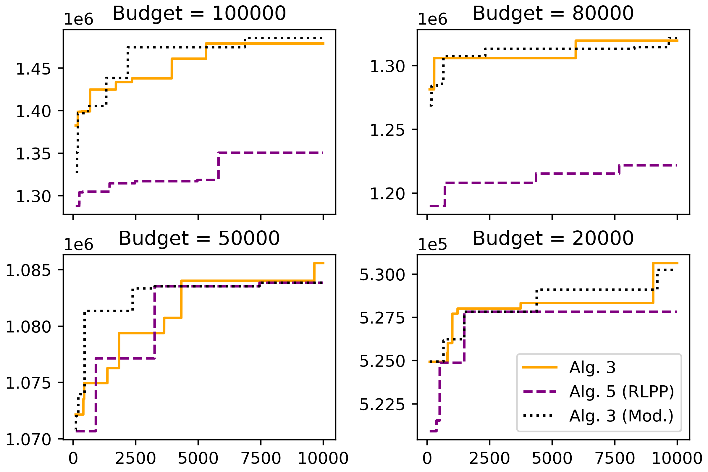
Figure 1: We compared three methods: Algorithm 5 (with $\epsilon=0.05$) from [21], Modified Algorithm 3 (which uses the same LP solution for rounding as Algorithm 5), and Algorithm 3. Note that Algorithm 3 always performs better than Algorithm 5 since they use the same realizations produced by the rounding process, which is based on the same LP solution.

4.1.3 Approximation Solution to GRLPP

In this subsection, we investigate the approximation solution to GRLPP.

As shown in [21, Appendix A.1], the LP relaxation of (3.1) can be solved with an approximation ratio of $\frac{1}{8}-\delta$ for any $\delta>0$.

It is also suggested that the same rounding process as in [21, Algorithm 1] can be applied based on the LP solution, resulting in an approximation ratio of $\frac{1}{8}\left(1-\frac{1}{e}\right)-\epsilon$ with a probability of violating the budget constraint bounded by $e^{-\epsilon^{2}k/3}$, where $k:=\frac{B}{\max_{l\in\mathcal{L}}c_{l}}$, as previously defined. However, the analysis and theoretical guarantee in [21] cannot be directly applied to this case since, when a passenger is assigned to a line, it can potentially generate different rewards, i.e., $v_{lp}^{(i)}\neq v_{lp}^{(i^{\prime})}$ for $i\neq i^{\prime}$. In this context, [21, Lemma B.1] cannot be used to demonstrate the approximation ratio because the ranking of rewards for a passenger assigned to different lines is stochastic rather than deterministic based on the randomized rounding process, which is a critical assumption in [21, Lemma B.1].

Nonetheless, as demonstrated in Theorem 3.2, Algorithm 1 and Algorithm 3 presented in this paper can be employed for randomized rounding based on the LP solution, yielding a solution to (3.1) with an approximation ratio of $\frac{1}{16}\left(1-\frac{1}{\sqrt{k}}\right)-\epsilon$ and $\frac{1}{16}\left(1-\frac{1}{\sqrt{k}}\right)\frac{k-1}{k}-\epsilon$ respectively.

4.2 Generalized Budgeted Multi-Visit Team Orienteering Problem

In this section, we demonstrate the application of our framework to construct approximation algorithms for the Generalized Budgeted Multi-Visit Team Orienteering Problem (GBMTOP), assuming the availability of an approximation algorithm for the corresponding single-vehicle orienteering problem. First, let us provide a formal definition of the problem.

Consider a complete undirected graph $G=(N\cup\{s,t\},E)$, where $N=\{n_{1},n_{2},\dots,n_{P}\}$ represents a set of $P$ nodes requiring service, $s$ denotes the source node, and $t$ indicates the destination node. Note that nodes $s$ and $t$ may or may not be co-located. An edge exists in $E$ between any two nodes in $N\cup\{s,t\}$.

There are $L>1$ heterogeneous vehicles available to serve the nodes in $N$, with all vehicles initially located at the source node $s$. Each vehicle $l$ must find a simple path $P_{l}$ from node $s$ to node $t$, with $1\leq l\leq L$. If $P_{l}$ crosses edge $e\in E$ or node $n_{p}\in N$, we say $e\in P_{l}$ or $p\in P_{l}$.

For each vehicle $l$, there are $m_{l}$ different modes, and it can choose one mode before departing from node $s$.

For $e\in E$, the time taken to traverse $e$ for vehicle $l$ is denoted by $d^{(l)}_{e}$. There is an upper bound $D^{(i)}_{l}$ for the time consumed by vehicle $l$ with mode $i$ on $P_{l}$, i.e.,

$$\sum_{e\in P_{l}}d^{(l)}_{e}\leq D^{(i)}_{l}.$$

For each node $n_{p}$, $p\in\{1,2,\dots,P\}$, it can be visited at most $\rho$ times, and each vehicle can visit a node at most once. Additionally, there is a reward $v^{(i)}_{lp}$ when vehicle $l$ with mode $i$ visits node $n_{p}$. In this context, each vehicle with the selected mode can represent one type of service, and each visit signifies that a node is served by the vehicle with the selected mode. Let $S=(S_{1},S_{2},\ldots,S_{m_{l}})$ be an assignment of nodes visited by vehicle $l$. When vehicle $l$ selects mode $i^{\prime}$, $S_{i}=\emptyset$ for all $i\neq i^{\prime}$, and $S_{i^{\prime}}$ is the set of all nodes visited by vehicle $l$ with mode $i^{\prime}$. A node assignment for vehicle $l$ is considered feasible if there exists a feasible path $P_{l}$ to visit all the nodes included in the assignment. Let $I_{l}$ be the collection of all feasible node assignments for vehicle $l$ across all possible modes. We say $S\in I_{l}$ when a feasible path $P_{l}$ exists to visit the nodes in $S$ by vehicle $l$ with the corresponding mode.

Furthermore, dispatching vehicle $l$ with the mode indicated by $S\in I_{l}$ incurs a cost $c_{lS}$, and there is a budget $B$ for it.

To solve GBMTOP, we must maximize the rewards produced by vehicle visits to nodes so as to satisfy all of the aforementioned constraints. Specifically, we can formulate it same as (3.1).

Consider that when $B=\infty$, $\rho=1$, $m_{l}=1$ for all $l$, and vehicles are homogeneous, GBMTOP simplifies to the regular team orienteering problem. In scenarios where only one vehicle with only one possible mode is accessible, the problem transforms into a classic single-vehicle orienteering problem.

The orienteering problem, along with its numerous variations, has been extensively studied in the literature [23, 16]. For metric graphs, Chekuri et al. [11] developed an approximation algorithm for the single-vehicle orienteering problem, achieving an approximation ratio of $\frac{1}{2}-\epsilon$, where the starting node $s$ and ending node $t$ can be different and $\epsilon$ is a given constant such that $0<\epsilon\leq 1$. In the context of the orienteering problem in Euclidean space, Chen and Har-Peled [12] introduced a Polynomial Time Approximation Scheme (PTAS), providing a $(1-\epsilon)$-approximate solution, where $\epsilon$ is a constant satisfying $0<\epsilon\leq 1$.

Additionally, research has been conducted on the team orienteering problem (TOP), which seeks to determine service tours for multiple vehicles, with each node visited by at most one vehicle. Various exact algorithms and metaheuristics for TOP and its variations have been proposed in the literature (see for example [8, 24, 17, 20]). Bock et al. [4] proposed a $\left(\frac{1}{3}-\epsilon\right)$-approximation algorithm for single-vehicle capacitated orienteering problems, in which the total demand of visited nodes does not exceed a given capacity bound. They further generalized this to a $3.53$-approximation algorithm for capacitated team orienteering problems with homogeneous vehicles. Xu et al. [25] presented an $\left(1-\frac{1}{e^{2+\epsilon}}\right)$-approximation algorithm for a generalized team orienteering problem (GTOP), which aims to find service paths for multiple homogeneous vehicles in a network such that the profit sum of serving the nodes in the paths is maximized, subject to the cost budget of each vehicle. It is important to note that, in GTOP, a node can be served by multiple vehicles.

To the best of our knowledge, GBMTOP has not been previously studied in the literature. The main distinctions between GBMTOP and the TOP variants are as follows: (i) the presence of budget constraints for dispatching vehicles, (ii) the allowance of heterogeneous vehicles, and (iii) the flexibility for vehicles to select distinct modes.

If we have a $\beta$-approximation algorithm for the single orienteering problem, we can use Algorithm 1 and Algorithm 3 to solve GBMTOP, provided that we can obtain a $\left(\beta-\delta\right)$-approximation solution to the dual of the LP relaxation of (3.1) in the context of GBMTOP. For details on how to obtain an approximation solution to the LP relaxation of (3.1) in the context of GBMTOP, please refer to Appendix E.

By employing Theorem 3.2, we can achieve a $\beta\left(1-\frac{1}{\sqrt{\rho+3}}\right)\left(1-\frac{1}{\sqrt{k}}\right)-\epsilon$ approximation. Chekuri et al. [11] discovered a $\left(\frac{1}{2}-\epsilon\right)$-approximation algorithm in an undirected weighted graph for general metrics. This result promptly leads to $\frac{1}{2}\left(1-\frac{1}{\sqrt{\rho+3}}\right)\left(1-\frac{1}{\sqrt{k}}\right)-\epsilon$ approximation algorithms for GBMTOP.

Naturally, we can also apply our framework to other variations of the orienteering problems. For instance, we can introduce the following constraints: each node $n_{p}$ requires service by vehicle $l$ with mode $i$ for $h^{(i)}_{lp}$ hours, each node can receive at most $\rho$ types of services, and each vehicle with mode $i$ can provide a maximum of $H^{(i)}_{l}$ hours for the services. Note that vehicle $l$ with mode $i$ must supply all the $h^{(i)}_{lp}$ hours of services to node $n_{p}$ to obtain the reward. Thus, by the approximation algorithm by [4] with an approximation ratio of $\frac{1}{3}-\epsilon$ for the capacitated orienteering problems, we can generate an $\left(\frac{1}{3}\left(1-\frac{1}{\sqrt{\rho+3}}\right)\left(1-\frac{1}{\sqrt{k}}\right)-\epsilon\right)$-approximation algorithm for the budgeted multi-visit orienteering problems with service hour constraints.

Appendix A Solve the relaxation

In this section we will show how to solve (3.3), which can be written as the following.

$$\underset{\{X_{lS}\}}{\max}~{}~{}~{}~{}~{}~{}~{} \sum_{p\in[P]}\sum_{l\in[L]}\sum_{S\in I_{l}:p\in S_{i}}v^{(i)}_{lp}X_{lS}$$ (A.1a)

$$s.t.~{}~{}~{}~{}~{}~{}~{}~{} \sum_{S\in I_{l}}X_{lS}\leq 1~{}~{}~{}~{}\forall l\in[L]$$ (A.1b)

$$\sum_{l\in[L]}\sum_{S\in I_{l}:p\in S}X_{lS}\leq\rho~{}~{}~{}~{}\forall p\in[P]$$ (A.1c)

$$\sum_{l\in[L]}\sum_{S\in I_{l}}c_{lS}X_{lS}\leq B-\epsilon$$ (A.1d)

$$X_{lS}\in[0,1]$$ (A.1e)

Its dual can be written as:

$$\underset{\{q_{l},\lambda_{p},\alpha_{1},\alpha_{2}\}}{\min}~{}~{}~{}~{}~{}~{}~{} \sum_{l\in[L]}q_{l}+\sum_{p\in[P]}\rho\lambda_{p}+B\alpha$$ (A.2a)

$$s.t~{}~{}~{}~{}~{}~{}~{}~{}~{}~{}~{} q_{l}+\alpha c_{l}\geq\sum_{p\in S_{i},i\in[m_{l}]}(v^{(i)}_{lp}-\lambda_{p}-\alpha c^{(i)}_{lp})~{}~{}~{}~{}~{}~{}\forall l\in[L],S\in I_{l}$$ (A.2b)

$$q_{l},\lambda_{p},\alpha\geq 0~{}~{}~{}\forall l\in[L],~{}p\in[P].$$ (A.2c)

The dual (A.2) has exponentially many constraints but polynomially many variables. Considering a point $(q_{l},\lambda_{p},\alpha~{}|~{}p\in[P])$, a $\beta$-approximation algorithm ($\beta\leq 1$) for the corresponding single-bin problem either returns a violated constraint or ensures that $(q_{l}/\beta,\lambda_{p},\alpha/\beta~{}|~{}p\in[P])$ is feasible for the current constraints of the dual. Following the same logic as [15, Lemma 2.2], for any $\delta\geq 0$, we can develop a polynomial-time $(\beta-\delta)$-approximation algorithm to solve the linear program (E.2) and, consequently, the linear program (E.1). Then, by replacing $\epsilon$ in (3.3) with $\frac{\epsilon}{2}$ and finding an appropriate $\delta$, we can find a $\beta$-approximation solution to (3.3).

Appendix B Proof for Theorem 3

Again, we define an algorithm that can be no better than Algorithm 3. Thus, its approximation ratio is also applicable to Algorithm 3.

Note that Step 5 and 6 are only used for analysis. Therefore, it is not necessary to round up $c_{l}$ like in Algorithm 2.

Algorithm 4.

1. Find a $\left(\beta-\epsilon\right)$-approximation solution to the relaxation of (3.1) and let $\widetilde{X}$ be the solution.

2. Reorder the bins so that

   $$\frac{\sum_{S\in I_{l}}\left(\widetilde{X}_{lS}\sum_{p\in S_{i}}v^{(i)}_{lp}\right)}{c_{l}\sum_{S\in I_{l}}\widetilde{X}_{lS}}\geq\frac{\sum_{S\in I_{l^{\prime}}}\left(\widetilde{X}_{l^{\prime}S}\sum_{p\in S_{i}}v_{l^{\prime}p}^{(i)}\right)}{c_{l^{\prime}}\sum_{S\in I_{l^{\prime}}}\widetilde{X}_{l^{\prime}S}}~{}~{}~{}~{}~{}~{}\mbox{ for }1\leq l<l^{\prime}\leq L.$$ (B.1)

   Note that here if the denominators are zeros, the corresponding numerators are also zeros, and the corresponding bins can be ignored in the following rounding process. Thus, we can define $\frac{0}{0}:=0$ in (3.14).

3. Independently for each $l\in[L]$, randomly flip a two-sided coin with probability $\sum_{S\in I_{l}}\widetilde{X}_{lS}$ as head. If the result is head, then $H_{l}=1$. Otherwise, $H_{l}=0$.

4. For each $l\in[L]$, $\widetilde{c}_{l}={c}_{l}H_{l}$, and its distribution can be written as

   $$P(\widetilde{c}_{l}=c)=\begin{cases}1-\sum_{S\in I_{l}}\widetilde{X}_{lS}&\text{if }c=0\\ \sum_{S\in I_{l}}\widetilde{X}_{lS}&\text{if }c={c}_{l}\end{cases}.$$

5. Create a generalized $\left(1-\frac{1}{\sqrt{k}}\right)$-conservative magician with a $k$ units of mana (we will refer to this as a type-0 magician).

6. The magician is presented with a sequence of $L$ type-0 boxes from box $1$ to box $L$. The distribution of $\widetilde{c}_{l}$ is written on type-0 box $l$. The amount of mana the magician will lose if type-0 box $l$ is opened and equal to the value of ${c}_{l}$. The magician will decide whether to open type-0 box $l$ following Definition 2.2. Let the decision variable be $Z_{l}$ such that $Z_{l}=1$ if the magician decides to open type-0 box $l$, and $Z_{l}=0$ otherwise.

7. Let $B_{0}=k$. Let $l$ be from $1$ to $L$. At $l$th iteration, if $B_{l}=B_{l-1}-{c}_{l}H_{l}\geq 0$, then let $\xi_{l}=1$. Otherwise, $\xi_{l}=0$.

8. Independently for each $l\in[L]$, if $\sum_{S\in I_{l}}\widehat{X}_{lS}=0$, then $H_{l}^{S}=0$ for each $S\in I_{l}$ (and in this case, $H_{l}=0$ with probability $1$). Otherwise, randomly select a set $S^{\prime}_{l}$ from $I_{l}$ following the distribution below:

   $$P({S^{\prime}}_{l}=S)=\frac{\widehat{X}_{lS}}{\sum_{S\in I_{l}}\widehat{X}_{lS}}\text{ for }S\in I_{l}.$$

   Then let $H_{l}^{S^{\prime}_{l}}=1$, and $H_{l}^{S}=0$ if $S\in I_{l}\backslash\{S^{\prime}_{l}\}$. Let $Z_{l}^{S}=H_{l}\cdot H_{l}^{S}$ for $S\in I_{l}$. If there exists $S\in I_{l}$ such that $Z_{l}^{S}=1$, then let $T_{l}=S$. Otherwise, $T_{l}=\emptyset$.

9. For each $l\in[L]$ and $p\in[P]$, define a random variable $\widetilde{Y}_{lp}:=\sum_{S\in I_{l};~{}p\in S}Z_{l}^{S}$. Its distribution can be written as

   $$P(\widetilde{Y}_{lp}=y)=\begin{cases}1-\sum_{S\in I_{l};~{}p\in S}\widetilde{X}_{lS}&\text{if }y=0\\ \sum_{S\in I_{l};~{}p\in S}\widetilde{X}_{lS}&\text{if }y=1\end{cases}.$$

10. For each $p\in[P]$, create a generalized $\left(1-\frac{1}{\sqrt{\rho+3}}\right)$-conservative magician with $\rho$ units of mana (called type-p magician). The magician of $p$ is presented with a sequence of $L$ type-$p$ boxes from box $L$ to box $1$. The distribution of $\widetilde{Y}_{lp}$ is written on type-$p$ box $l$. The amount of mana the magician will lose if open type-$p$ box $l$ is equal to the value of $\widetilde{Y}_{lp}$. The magician will decide whether to open type-$p$ box $l$ following Definition 2.2. Let the (random) decision variable be $Z_{l}^{p}$, i.e., $Z_{l}^{p}=1$ if the magician for $p$ decides to open type-$p$ box $l$, and $Z_{l}^{p}=0$ otherwise.

11. If $p\in T_{l}$, $\xi_{l}=1$ and $Z_{l}^{p}=1$, then we assign $p$ to $l$ in the final solution.

We first show that the $Z_{l}^{S}$ defined in Algorithm 4 is actually equivalent to the $Z_{l}^{S}$ defined in Algorithm 2.

Lemma B.1.

For each $l\in[L]$, the joint distribution of $\{Z_{l}^{S}\}_{\{S\in I_{l}\}}$ is

$$P(Z_{l}^{S}=1,Z_{l}^{S^{\prime}}=0\mbox{ for each }S\in I_{l},~{}S^{\prime}\in I_{l}\backslash\{S\})=\widehat{X}_{l}^{S},$$ (B.2)

$$P(Z_{l}^{S}=0\mbox{ for each }S\in I_{l})=1-\sum_{S\in I_{l}}\widehat{X}_{l}^{S}.$$ (B.3)

Proof.

By Step 8, $Z_{l}^{S}=H_{l}\cdot H_{l}^{S}$. We know that $H_{l}$ and $H_{l}^{S}$ are independent by their definitions. Thus, we have

$$P(Z_{l}^{S}=1,Z_{l}^{S^{\prime}}=0\mbox{ for each }S^{\prime}\in I_{l}\backslash\{S\})$$ (B.4)

$$= P(H_{l}=1)P(H_{l}^{S}=1,H_{l}^{S^{\prime}}=0\mbox{ for each }S^{\prime}\in I_{l}\backslash\{S\})~{}~{}~{}\mbox{for $S\in I_{l}$}.$$ (B.5)

$$P(Z_{l}^{S}=0\mbox{ for each }S\in I_{l})=P(H_{l}=0).$$ (B.6)

Then we can substitute the distributions of $H_{l}$ and $H_{l}^{S}$ and finish the proof. ∎

Remark B.2.

The reason why we do not directly define $Z_{l}^{S}$ in Algorithm 4 as in Algorithm 2 is that this makes the analysis clearer from our perspective.

Again, we can prove the following independence results in a similar way as Lemma 3.5.

Lemma B.3.

We have that $Z_{l}^{p}$ is independent to $\xi_{l}$, $Z_{l}$ and $Z_{l}^{S}$ for each $l\in[L]$ and $S\in I_{l}$.

We will also use the following lemma to prove the approximation ratio for Algorithm 4.

Lemma B.4.

$$\mathbb{E}\left[\sum_{l\in[L]}\sum_{p\in[P]}\sum_{S\in I_{l}:p\in S_{i}}v^{(i)}_{lp}Z_{l}^{S}\cdot\xi_{l}\right]$$ (B.7)

$$\geq \frac{k-1}{k}\left(1-\frac{1}{\sqrt{k}}\right)\sum_{l\in[L]}\sum_{p\in[P]}\sum_{S\in I_{l}:p\in S_{i}}v^{(i)}_{lp}\widehat{X}_{lS}$$ (B.8)

With these results, we can demonstrate the claimed approximation ratio of Algorithm 4.

Theorem B.5.

The solution given by Algorithm 4 is feasible. The expected objective value of the solution is at least $\beta\left(1-\frac{1}{\sqrt{\rho+3}}\right)\frac{k-1}{k}\left(1-\frac{1}{\sqrt{k}}\right)-\epsilon$ of the optimal value of the solution to the relaxation of (3.3).

Proof.

By the design of the algoithm, we can prove that the following two inequalities are guaranteed:

$$\sum_{l\in[L]}\xi_{l}c_{l}\sum_{S\in I_{l}}Z_{l}^{S}\leq k$$

$$\sum_{l\in[L]}\xi_{l}Z_{l}^{p}\sum_{S\in I_{l}:~{}p\in S}Z_{l}^{S}\leq\sum_{l\in[L]}Z_{l}^{p}\sum_{S\in I_{l}:~{}p\in S}Z_{l}^{S}\leq\rho\mbox{ for each }p\in[P].$$

Thus the final solution satisfies that the budget is not breached, and item $p$ can be assigned to at most $\rho$ bins. Step 3 guarantees that each bin can have at most one copy of each item since each $S\in I_{l}$ contains at most one copy of each item.

We will prove the rest of the theorem.

$$~{}~{}~{}~{}\mathbb{E}\left[\sum_{l\in[L]}\sum_{S\in I_{l}}\sum_{p\in S_{i}}v^{(i)}_{lp}Z_{l}^{p}Z_{l}^{S}\cdot\xi_{l}\right]$$ (B.9)

$$=\sum_{l\in[L]}\sum_{S\in I_{l}}\sum_{p\in S_{i}}v^{(i)}_{lp}\mathbb{E}\left[Z_{l}^{p}Z_{l}^{S}\cdot\xi_{l}\right]$$ (B.10)

$$=\sum_{l\in[L]}\sum_{S\in I_{l}}\sum_{p\in S_{i}}v^{(i)}_{lp}\mathbb{E}\left[Z_{l}^{p}\right]\mathbb{E}\left[Z_{l}^{S}\cdot\xi_{l}\right]$$ (B.11)

$$=\sum_{l\in[L]}\sum_{S\in I_{l}}\sum_{p\in S_{i}}v^{(i)}_{lp}\left(1-\frac{1}{\sqrt{\rho+3}}\right)\mathbb{E}\left[Z_{l}^{S}\cdot\xi_{l}\right]$$ (B.12)

$$\geq\left(1-\frac{1}{\sqrt{\rho+3}}\right)\mathbb{E}\left[\sum_{l\in[L]}\sum_{S\in I_{l}}\sum_{p\in S_{i}}v^{(i)}_{lp}Z_{l}^{S}\cdot\xi_{l}\right]$$ (B.13)

$$\geq\left(1-\frac{1}{\sqrt{\rho+3}}\right)\frac{k-1}{k}\left(1-\frac{1}{\sqrt{k}}\right)\sum_{l\in[L]}\sum_{p\in[P]}\sum_{S\in I_{l}:p\in S_{i}}v^{(i)}_{lp}\widehat{X}_{lS}$$ (B.14)

Eq. (B.11) is due to Lemma B.3, Inequality (B.12) is by Theorem 2.3, and Inequality (B.14) is based on Lemma B.4. ∎

The final step to finish the proof of Theorem B.5 is to prove Lemma B.4.

The following independence result can be checked based on the design of Algorithm 4.

Lemma B.6.

We have that $Z_{l}$ and $Z_{l}^{S}$ are mutually independent for each $l\in[L]$ and $S\in I_{l}$. Moreover, $H_{l}^{S}$ is independent to $Z_{l}$ and $H_{l}$.

Then we can derive the following lemma based on Lemma B.1, Lemma B.6 and Theorem 2.3 in the same way as the proof of Theorem 3.2.

Lemma B.7.

$$\mathbb{E}\left[\sum_{l\in[L]}\sum_{p\in[P]}\sum_{S\in I_{l}:p\in S_{i}}v^{(i)}_{lp}Z_{l}^{S}\cdot Z_{l}\right]\geq \left(1-\frac{1}{\sqrt{k}}\right)\sum_{l\in[L]}\sum_{p\in[P]}\sum_{S\in I_{l}:p\in S_{i}}v^{(i)}_{lp}\widehat{X}_{lS}$$ (B.15)

Proof.

$$\mathbb{E}\left[\sum_{l\in[L]}\sum_{p\in[P]}\sum_{S\in I_{l}:p\in S_{i}}v^{(i)}_{lp}Z_{l}^{S}\cdot Z_{l}\right]$$ (B.16)

$$= \sum_{l\in[L]}\sum_{p\in[P]}\sum_{S\in I_{l}:p\in S_{i}}v^{(i)}_{lp}\mathbb{E}\left[Z_{l}^{S}\cdot Z_{l}\right]$$ (B.17)

$$= \sum_{l\in[L]}\sum_{p\in[P]}\sum_{S\in I_{l}:p\in S_{i}}v^{(i)}_{lp}\mathbb{E}\left[Z_{l}^{S}\right]\cdot\mathbb{E}\left[Z_{l}\right]$$ (B.18)

$$= \left(1-\frac{1}{\sqrt{k}}\right)\sum_{l\in[L]}\sum_{p\in[P]}\sum_{S\in I_{l}:p\in S_{i}}v^{(i)}_{lp}\widehat{X}_{lS}$$ (B.19)

∎

We now proceed with the proof of the following result, which immediately implies Lemma B.4 after combining with Lemma B.7.

Lemma B.8.

$$\mathbb{E}\left[\sum_{l\in[L]}\sum_{p\in[P]}\sum_{S\in I_{l}:p\in S_{i}}v^{(i)}_{lp}Z_{l}^{S}\cdot\xi_{l}\right]\geq \frac{k-1}{k}\mathbb{E}\left[\sum_{l\in[L]}\sum_{p\in[P]}\sum_{S\in I_{l}:p\in S_{i}}v^{(i)}_{lp}Z_{l}^{S}\cdot Z_{l}\right]$$ (B.20)

Proof.

Given $\{\widehat{H}_{l}\}_{l\in[L]}$ and $\{\widehat{Z}_{l}\}_{l\in[L]}$ as a possible realization of $\{H_{l}\}_{l\in[L]}$ and $\{Z_{l}\}_{l\in[L]}$, it suffices to show that

$$\mathbb{E}\left[\sum_{l\in[L]}\sum_{p\in[P]}\sum_{S\in I_{l}:p\in S_{i}}v^{(i)}_{lp}Z_{l}^{S}\cdot\xi_{l}\Big{|}{H}_{l}=\widehat{H}_{l},Z_{l}=\widehat{Z_{l}},\mbox{ for all }l\in[L]\right]$$

$$\geq \frac{k-1}{k}\mathbb{E}\left[\sum_{l\in[L]}\sum_{p\in[P]}\sum_{S\in I_{l}:p\in S_{i}}v^{(i)}_{lp}Z_{l}^{S}\cdot Z_{l}\Big{|}{H}_{l}=\widehat{H}_{l},Z_{l}=\widehat{Z_{l}},\mbox{ for all }l\in[L]\right].$$

Note that given $\{\widehat{H}_{l}\}_{l\in[L]}$, the realization of $\{{\xi}_{l}\}_{l\in[L]}$ is also determined. Let it be $\{\widehat{\xi}_{l}\}_{l\in[L]}$. We first rewrite the two terms on both sides of the above inequality based on the independence results from Lemma B.6.

$$\mathbb{E}\left[\sum_{l\in[L]}\sum_{p\in[P]}\sum_{S\in I_{l}:p\in S_{i}}v^{(i)}_{lp}Z_{l}^{S}\cdot\xi_{l}\Big{|}{H}_{l}=\widehat{H}_{l},Z_{l}=\widehat{Z_{l}}\mbox{ for all }l\in[L]\right]$$ (B.21)

$$= \mathbb{E}\left[\sum_{l\in[L]}\sum_{p\in[P]}\sum_{S\in I_{l}:p\in S_{i}}v^{(i)}_{lp}H_{l}^{S}\cdot\widehat{H}_{l}\cdot\widehat{\xi}_{l}\right]$$ (B.22)

$$= \sum_{l\in[L]}\sum_{p\in[P]}\sum_{S\in I_{l}:p\in S_{i}}v^{(i)}_{lp}\cdot\widehat{H}_{l}\cdot\widehat{\xi}_{l}\cdot\mathbb{E}\left[H_{l}^{S}\right]$$ (B.23)

$$= \sum_{l\in[L]}\widehat{H}_{l}\cdot\widehat{\xi}_{l}\sum_{p\in[P]}\sum_{S\in I_{l}:p\in S_{i}}v^{(i)}_{lp}\cdot\mathbb{E}\left[H_{l}^{S}\right]$$ (B.24)

$$\mathbb{E}\left[\sum_{l\in[L]}\sum_{p\in[P]}\sum_{S\in I_{l}:p\in S_{i}}v^{(i)}_{lp}Z_{l}^{S}\cdot Z_{l}\Big{|}{H}_{l}=\widehat{H}_{l},Z_{l}=\widehat{Z_{l}}\mbox{ for all }l\in[L]\right]$$ (B.25)

$$= \mathbb{E}\left[\sum_{l\in[L]}\sum_{p\in[P]}\sum_{S\in I_{l}:p\in S_{i}}v^{(i)}_{lp}H_{l}^{S}\cdot\widehat{H}_{l}\cdot\widehat{Z_{l}}\right]$$ (B.26)

$$= \sum_{l\in[L]}\sum_{p\in[P]}\sum_{S\in I_{l}:p\in S_{i}}v^{(i)}_{lp}\cdot\widehat{H}_{l}\cdot\widehat{Z_{l}}\cdot\mathbb{E}\left[H_{l}^{S}\right]$$ (B.27)

$$= \sum_{l\in[L]}\widehat{H}_{l}\cdot\widehat{Z_{l}}\sum_{p\in[P]}\sum_{S\in I_{l}:p\in S_{i}}v^{(i)}_{lp}\cdot\mathbb{E}\left[H_{l}^{S}\right].$$ (B.28)

(B.22) and (B.26) are based on Lemma B.6 and the definition in Step 8 that $Z_{l}^{S}=H_{l}\cdot H_{l}^{S}$.

Let $\widehat{\Lambda}_{1}:=\{l\in[L]:\widehat{H}_{l}=1\}$, $\widehat{\Lambda}_{2}:=\{l\in\widehat{\Lambda}_{1}:\widehat{Z}_{l}=1\}$, and $\widehat{\Lambda}_{3}:=\{l\in\widehat{\Lambda}_{1}:\widehat{\xi}_{l}=1\}$. For simplicity, define $\beta_{l}:=\sum_{p\in[P]}\sum_{S\in I_{l}:p\in S_{i}}v^{(i)}_{lp}\cdot\mathbb{E}\left[H_{l}^{S}\right]$. Then we can rewrite the above equations further

$$\sum_{l\in[L]}\widehat{H}_{l}\cdot\widehat{Z_{l}}\sum_{p\in[P]}\sum_{S\in I_{l}:p\in S_{i}}v^{(i)}_{lp}\cdot\mathbb{E}\left[H_{l}^{S}\right]=\sum_{l\in\widehat{\Lambda}_{2}}\sum_{p\in[P]}\sum_{S\in I_{l}:p\in S_{i}}v^{(i)}_{lp}\cdot\mathbb{E}\left[H_{l}^{S}\right]=\sum_{l\in\widehat{\Lambda}_{2}}\beta_{l}$$

$$\sum_{l\in[L]}\widehat{H}_{l}\cdot\widehat{\xi}_{l}\sum_{p\in[P]}\sum_{S\in I_{l}:p\in S_{i}}v^{(i)}_{lp}\cdot\mathbb{E}\left[H_{l}^{S}\right]=\sum_{l\in\widehat{\Lambda}_{3}}\sum_{p\in[P]}\sum_{S\in I_{l}:p\in S_{i}}v^{(i)}_{lp}\cdot\mathbb{E}\left[H_{l}^{S}\right]=\sum_{l\in\widehat{\Lambda}_{3}}\beta_{l}$$

To finish the proof of the claim, it suffices to prove that

$$\sum_{l\in\widehat{\Lambda}_{3}}\beta_{l}\geq\frac{k-1}{k}\sum_{l\in\widehat{\Lambda}_{2}}\beta_{l}.$$

If $\widehat{\Lambda}_{2}\subseteq\widehat{\Lambda}_{3}$, then this is straightforward. Otherwise, let $l_{\max}=\max_{l\in\widehat{\Lambda}_{3}}l$. Then by definition of $\xi$, $\widehat{\Lambda}_{3}=\{l\in\widehat{\Lambda}_{1}:\widehat{\xi}_{l}=1,l\leq l_{\max}\}$. Let $c_{0}=k-\sum_{l\in\widehat{\Lambda}_{3}}c_{l}$. Then we have $0\leq c_{0}<1$, and $c_{0}+\sum_{l\in\widehat{\Lambda}_{3}}{c}_{l}=k$. The magician guarantees that $\sum_{l\in\widehat{\Lambda}_{2}}c_{l}\leq k$. By the definition of $\{\widehat{Z}_{l}\}_{l\in[L]}$ and $\{\widehat{\xi}_{l}\}_{l\in[L]}$, we have $\min_{l\in\widehat{\Lambda}_{2}\backslash\widehat{\Lambda}_{3}}l>\max_{l\in\widehat{\Lambda}_{3}}l$. By Step 2 in Algorithm 4, we have

$$\frac{\sum_{S\in I_{l}}\left(\widehat{X}_{lS}\sum_{p\in S_{i}}v^{(i)}_{lp}\right)}{c_{l}\sum_{S\in I_{l}}\widehat{X}_{lS}}\geq\frac{\sum_{S\in I_{l^{\prime}}}\left(\widehat{X}_{l^{\prime}S}\sum_{p\in S_{i}}v^{(i)}_{l^{\prime}p}\right)}{c_{l^{\prime}}\sum_{S\in I_{l^{\prime}}}\widehat{X}_{l^{\prime}S}}~{}~{}~{}~{}~{}~{}\mbox{ for }1\leq l<l^{\prime}\leq L.$$ (B.29)

It implies that

$$\frac{\sum_{S\in I_{l}}\left(\widehat{X}_{lS}\sum_{p\in S_{i}}v^{(i)}_{lp}\right)}{c_{l}\sum_{S\in I_{l}}\widehat{X}_{lS}}=\frac{1}{c_{l}}\sum_{p\in[P]}\sum_{S\in I_{l}:p\in S_{i}}v^{(i)}_{lp}\cdot\mathbb{E}\left[H_{l}^{S}\right]=\frac{1}{c_{l}}\beta_{l}$$

$$\geq \frac{\sum_{S\in I_{l^{\prime}}}\left(\widehat{X}_{l^{\prime}S}\sum_{p\in S_{i}}v^{(i)}_{l^{\prime}p}\right)}{c_{l^{\prime}}\sum_{S\in I_{l^{\prime}}}\widehat{X}_{l^{\prime}S}}=\frac{1}{c_{l^{\prime}}}\sum_{p\in[P]}\sum_{S\in I_{l^{\prime}}:p\in S_{i}}v^{(i)}_{l^{\prime}p}\cdot\mathbb{E}\left[H_{l^{\prime}}^{S}\right]=\frac{1}{c_{l^{\prime}}}\beta_{l^{\prime}}$$

$$\mbox{ for }1\leq l<l^{\prime}\leq L.$$

Combining all of these implies that

$$\frac{\beta_{l_{\max}}}{c_{l_{\max}}}\cdot c_{0}+\sum_{l\in\widehat{\Lambda}_{3}}\beta_{l}\geq\sum_{l\in\widehat{\Lambda}_{2}}\beta_{l}.$$

Also, since $0\leq c_{0}<1$, we have

$$\sum_{l\in\widehat{\Lambda}_{3}}\beta_{l}\geq\frac{k-1}{k}\left(\frac{\beta_{l_{\max}}}{c_{l_{\max}}}\cdot c_{0}+\sum_{l\in\widehat{\Lambda}_{3}}\beta_{l}\right)\geq\frac{k-1}{k}\sum_{l\in\widehat{\Lambda}_{2}}\beta_{l}.$$

This finishes the proof.

∎

Appendix C Hardness result for RLPP

Definition C.1.

Given a set of $n$ elements: $G=\{p_{1},\ldots,p_{n}\}$, and a collection of subsets of $[P]$: $\mathcal{F}:=\{G_{1},G_{2},\ldots,G_{L}\}$, max $k$-cover is the problem of selecting $k$ sets from $\mathcal{F}$ such that their union contains as many elements as possible.

The following hardness result has been proven in [13].

Theorem C.2.

For any $\epsilon>0$ and any positive integer $U$, there is always an integer $k$ such that $k\geq U$ and max $k$-cover problem cannot be approximated in polynomial time within an approximation ratio of $(1-\frac{1}{e}+\epsilon)$, unless $P=NP$.

Proof of Theorem 4.2.

Given an instance of max-$k$ cover problem with $G$ and $\mathcal{F}$ as defined in Definition C.1, it suffices to create an equivalent RLPP problem with $k=\frac{B}{\max_{l}c_{l}}$. We first create a complete graph with $2n$ vertices $\{o_{1,1},o_{1,2},o_{2,1},o_{2,2},\ldots,o_{n,1},o_{n,2}\}$. Without loss of generality, let the set $G$ represents the set of travelers in the created graph. Assume that traveler $p_{i}$ needs to go from $o_{i,1}$ to $o_{i,2}$ for all $i\in\{1,\ldots,n\}$. For a set $G_{j}:=\{p_{j_{1}},\ldots,p_{j_{|G_{j}|}}\}\in\mathcal{F}$, where $j_{1}\leq j_{2}\leq\ldots\leq j_{|G_{j}|}$, create a line $j$ with capacity $1$ in the following way. Include the edges connecting $o_{j_{i},1}$ and $o_{j_{i},2}$ for $i\in\{1,\ldots,|G_{j}|\}$, and the edges connecting $o_{j_{i},2}$ and $o_{j_{i+1},1}$ for $i\in\{1,\ldots,|G_{j}|-1\}$ so that this is a connected line. Then we set $c_{l}=1$ and $v_{lp}=1$ for each $l\in\{1,\ldots,L\}$ and $p\in G$. This is equivalent to the given max $k$-cover instance if we set the budget to be $k$. ∎

Appendix D Comparison between Algorithm 1 and the method in [21]

Here we first restate the method in [21] while omitting the aggregation step.

Algorithm 5.

1. Let $\widehat{X}$ be the solution to the LP relaxation of (3.3).

2. Independently for each $l\in[L]$, randomly select a set $T_{l}$ from $I_{l}\cup\{\emptyset\}$ following the distribution below:

   $$P({T}_{l}=S)=\begin{cases}1-\sum_{S\in I_{l}}\widehat{X}_{lS}&\text{if }S=\emptyset\\ \widehat{X}_{lS}&\text{if }S\in I_{l}\end{cases}.$$

   Let the (random) decision variable be $Z_{l}^{S}$, i.e., $Z_{l}^{S}=1$ if $S=T_{l}$, and $Z_{l}^{S}=0$ otherwise for $S\in I_{l}\cup\{\emptyset\}$.

3. Temporarily assign all the elements in $T_{l}$ to bin $l$ for each $l\in[L]$.

4. For $p\in[P]$, we remove each item $p$ that is assigned to more than $\rho$ bins from all but the $\rho$ bins with highest rewards $v_{lp}$ it is assigned to.

5. Open all the lines that have been assigned with at least one passenger, and close all the other lines. If this assignment does not exceed the budget, then we take this assignment as the final solution.

Appendix E Approximate the LP relaxation of (3.1) in the context of GBMTOP

The LP relaxation can be written as the following.

$$\underset{\{X_{lS}\}}{\max}~{}~{}~{}~{}~{}~{}~{} \sum_{p\in[P]}\sum_{l\in[L]}\sum_{S\in I_{l}:p\in S_{i}}v^{(i)}_{lp}X_{lS}$$ (E.1a)

$$s.t.~{}~{}~{}~{}~{}~{}~{}~{} \sum_{S\in I_{l}}X_{lS}\leq 1~{}~{}~{}~{}\forall l\in[L]$$ (E.1b)

$$\sum_{l\in[L]}\sum_{S\in I_{l}:p\in S}X_{lS}\leq\rho~{}~{}~{}~{}\forall p\in[P]$$ (E.1c)

$$\sum_{l\in[L]}\left(\sum_{S\in I_{l}}c_{lS}X_{lS}\right)\leq B$$ (E.1d)

$$X_{lS}\in[0,1]$$ (E.1e)

Its dual can be written as:

$$\underset{\{q_{l},\lambda_{p},\alpha\}}{\min}~{}~{}~{}~{}~{}~{}~{} \sum_{l\in[L]}q_{l}+\sum_{p\in[P]}\rho\lambda_{p}+B\alpha$$ (E.2a)

$$s.t~{}~{}~{}~{}~{}~{}~{}~{}~{}~{}~{} q_{l}+\alpha c_{lS}\geq\sum_{p\in S_{i},i\in[m_{l}]}(v^{(i)}_{lp}-\lambda_{p})~{}~{}~{}~{}~{}~{}\forall l\in[L],S\in I_{l}$$ (E.2b)

$$q_{l},\lambda_{p},\alpha\geq 0~{}~{}~{}\forall l\in[L],~{}p\in[P].$$ (E.2c)

Given a $\beta$-approximation algorithm to single-vehicle orienteering problem, for each mode $i$, we apply it to find an $s-t$ path that adheres to the constraints provided by the definition of single-vehicle orienteering problems in order to maximize the accumulated rewards for each vehicle $l$ with mode $i$. It is important to note that the reward generated by vehicle $l$ with mode $i$ visiting node $n_{p}$ is given by $v^{(i)}_{lp}-\lambda_{p}$. If the reward is negative, we simply remove the corresponding node when solving the orienteering problem.

Considering a point $(q_{l},\lambda_{p},\alpha~{}|~{}p\in[P])$, a $\beta$-approximation algorithm for the orienteering problem either returns a violated constraint or ensures that $(q_{l}/\beta,\lambda_{p},\alpha/\beta~{}|~{}p\in[P])$ is feasible for the current constraints of the dual. Following the same logic as [15, Lemma 2,2], for any $\delta\geq 0$, we can develop a polynomial-time $(\beta-\delta)$-approximation algorithm to solve the linear program (E.2).

References

- [1] Saeed Alaei. Bayesian combinatorial auctions: Expanding single buyer mechanisms to many buyers. SIAM Journal on Computing, 43(2):930–972, 2014.
- [2] Saeed Alaei, MohammadTaghi Hajiaghayi, and Vahid Liaghat. The online stochastic generalized assignment problem. In Approximation, Randomization, and Combinatorial Optimization. Algorithms and Techniques, pages 11–25. Springer, 2013.
- [3] Marco Bender, Clemens Thielen, and Stephan Westphal. Packing items into several bins facilitates approximating the separable assignment problem. Information Processing Letters, 115(6-8):570–575, 2015.
- [4] Adrian Bock and Laura Sanità. The capacitated orienteering problem. Discrete Applied Mathematics, 195:31–42, 2015.
- [5] Geoff Boeing. Osmnx: A python package to work with graph-theoretic openstreetmap street networks. Journal of Open Source Software, 2(12), 2017.
- [6] Ralf Borndörfer, Martin Grötschel, and Marc E Pfetsch. A column-generation approach to line planning in public transport. Transportation Science, 41(1):123–132, 2007.
- [7] Ralf Borndörfer and Marika Karbstein. A direct connection approach to integrated line planning and passenger routing. In 12th Workshop on algorithmic approaches for transportation modelling, optimization, and systems. Schloss Dagstuhl-Leibniz-Zentrum fuer Informatik, 2012.
- [8] Sylvain Boussier, Dominique Feillet, and Michel Gendreau. An exact algorithm for team orienteering problems. 4or, 5:211–230, 2007.
- [9] Gruia Calinescu, Chandra Chekuri, Martin Pal, and Jan Vondrák. Maximizing a monotone submodular function subject to a matroid constraint. SIAM Journal on Computing, 40(6):1740–1766, 2011.
- [10] Chandra Chekuri and Sanjeev Khanna. A polynomial time approximation scheme for the multiple knapsack problem. SIAM Journal on Computing, 35(3):713–728, 2005.
- [11] Chandra Chekuri, Nitish Korula, and Martin Pál. Improved algorithms for orienteering and related problems. ACM Transactions on Algorithms (TALG), 8(3):1–27, 2012.
- [12] Ke Chen and Sariel Har-Peled. The euclidean orienteering problem revisited. SIAM Journal on Computing, 38(1):385–397, 2008.
- [13] Uriel Feige. A threshold of ln n for approximating set cover. Journal of the ACM (JACM), 45(4):634–652, 1998.
- [14] Uriel Feige and Jan Vondrak. Approximation algorithms for allocation problems: Improving the factor of 1-1/e. In 2006 47th Annual IEEE Symposium on Foundations of Computer Science (FOCS’06), pages 667–676. IEEE, 2006.
- [15] Lisa Fleischer, Michel X Goemans, Vahab S Mirrokni, and Maxim Sviridenko. Tight approximation algorithms for maximum separable assignment problems. Mathematics of Operations Research, 36(3):416–431, 2011.
- [16] Aldy Gunawan, Hoong Chuin Lau, and Pieter Vansteenwegen. Orienteering problem: A survey of recent variants, solution approaches and applications. European Journal of Operational Research, 255(2):315–332, 2016.
- [17] Saïd Hanafi, Renata Mansini, and Roberto Zanotti. The multi-visit team orienteering problem with precedence constraints. European journal of operational research, 282(2):515–529, 2020.
- [18] Ariel Kulik, Hadas Shachnai, and Tami Tamir. Approximations for monotone and nonmonotone submodular maximization with knapsack constraints. Mathematics of Operations Research, 38(4):729–739, 2013.
- [19] Karl Nachtigall and Karl Jerosch. Simultaneous network line planning and traffic assignment. In 8th Workshop on Algorithmic Approaches for Transportation Modeling, Optimization, and Systems (ATMOS’08). Schloss Dagstuhl-Leibniz-Zentrum für Informatik, 2008.
- [20] Christos Orlis, Nicola Bianchessi, Roberto Roberti, and Wout Dullaert. The team orienteering problem with overlaps: An application in cash logistics. Transportation Science, 54(2):470–487, 2020.
- [21] Noémie Périvier, Chamsi Hssaine, Samitha Samaranayake, and Siddhartha Banerjee. Real-time approximate routing for smart transit systems. Proceedings of the ACM on Measurement and Analysis of Computing Systems, 5(2):1–30, 2021.
- [22] Lionel Adrian Silman, Zeev Barzily, and Ury Passy. Planning the route system for urban buses. Computers & operations research, 1(2):201–211, 1974.
- [23] Pieter Vansteenwegen, Wouter Souffriau, and Dirk Van Oudheusden. The orienteering problem: A survey. European Journal of Operational Research, 209(1):1–10, 2011.
- [24] Thibaut Vidal, Nelson Maculan, Luiz Satoru Ochi, and Puca Huachi Vaz Penna. Large neighborhoods with implicit customer selection for vehicle routing problems with profits. Transportation Science, 50(2):720–734, 2016.
- [25] Wenzheng Xu, Weifa Liang, Zichuan Xu, Jian Peng, Dezhong Peng, Tang Liu, Xiaohua Jia, and Sajal K Das. Approximation algorithms for the generalized team orienteering problem and its applications. IEEE/ACM Transactions on Networking, 29(1):176–189, 2020.