Parallel Path Progression DAG Scheduling

Abstract

To satisfy the increasing performance needs of modern cyber-physical systems, multiprocessor architectures are increasingly utilized. To efficiently exploit their potential parallelism in hard real-time systems,

appropriate task models and scheduling algorithms that allow providing timing guarantees are required. Such scheduling algorithms and the corresponding worst-case response time analyses usually suffer from resource over-provisioning due to pessimistic analyses based on worst-case assumptions. Hence, scheduling algorithms and analysis with high resource efficiency are required. A prominent parallel task model is the directed-acyclic-graph (DAG) task model, where precedence constrained subjobs express parallelism.

This paper studies the real-time scheduling problem of sporadic arbitrary-deadline DAG tasks. We propose a path parallel progression scheduling property with only two distinct subtask priorities, which allows to track the execution of a collection of paths simultaneously. This novel approach significantly improves the state-of-the-art response time analyses for parallel DAG tasks for highly parallel DAG structures. Two hierarchical scheduling algorithms are designed based on this property, extending the parallel path progression properties and improving the response time analysis for sporadic arbitrary-deadline DAG task sets.

I Introduction

Modern cyber-physical systems have gradually shifted from uniprocessor to multiprocessor systems in order to deal with thermal and energy constraints, as well as the computational demands of increasingly complex applications, like control, perception algorithms, or video processing algorithms. This shift poses multiple challenges for the real-time verification, e.g., how to efficiently utilize the parallelism provided by multiprocessors for task sets with inter- and intra-task parallelism while guaranteeing that each task meets its deadline. While inter-task parallelism refers to the parallel execution of distinct tasks, each of which executes sequentially, intra-task parallelism refers to the parallel execution of a single task. Intra-task parallelism requires task models with subtask level granularity that can be scheduled in parallel, e.g., Fork-join models [23], synchronous parallel task models, or DAG (directed-acyclic graph) based task models.

A plethora of real-time scheduling algorithms and response time analyses thereof have been proposed, e.g., for generalized parallel task models [29], and for DAG (directed-acyclic graph) based task models [17, 12, 35, 14, 15, 2, 4, 26]. For DAG-based task models, improvements in the response time analyses can be categorized into analyses that improve inter-task interference, e.g., in [12, 14], or intra-task interference as e.g., in [24, 17, 18, 35]. In general, intra-task interference analyses build upon the interference analysis along the execution of the envelope (or critical path). The envelope (or critical path) of a DAG is a schedule-dependent sequence of subjobs of the DAG. The sequence starts with the last finishing subjob in a concrete schedule and is iteratively composed by choosing the subjob that finishes latest among all directly preceding subjobs of the current subjob under consideration. When no further predecessors exist, the envelope is complete. Since these subjobs envelope the execution of the DAG, the interference of the execution of this sequence (or path) bounds the response time. In federated scheduling [24], the intra-task interference of the envelope execution is upper-bounded by the workload of the non-envelope subjobs divided by the number of processors. The corresponding response time analysis requires no information about the internal structure of the DAG except for the total workload and the longest path.

This analysis was improved by He et al. [17], who proposed a specific intra-node priority assignment for list-scheduling that must respect the topological ordering of the nodes within the DAG. This priority assignment and the inspection of the DAG structure results in a less pessimistic upper-bound for a task’s self-interference of the envelope path compared to federated scheduling. These results are further improved and extended by Zhao et al. [35], where subjob dependencies are explicitly considered along the execution of the envelope path to more accurately bound self-interference. Most recently, He et al. [18] improve their prior work by lifting the topological order restrictions in their intra-node priority assignments, which further improved the results by Zhao et al. [35].

In contrast to the state-of-the-art, we consider the progress of many parallel paths instead of only the envelope in the response time analysis. The number of parallel paths can amount to the degree of maximum parallelism, i.e., the number of processors. Since paths, i.e., a sequence of directly preceding subtasks, inherently limit the parallelism of a DAG, a path-based analysis instead of a subtask-based analysis is beneficial. More precisely, inversely to prior approaches, we do not track the execution progress by the analysis of envelope path interference, but track analyzable simultaneous progress of a collection of many parallel paths alongside the envelope path using intra-task prioritization. By virtue of this novel approach, we only have to account for the interference of subjobs that do not belong to any of these parallel paths for a response time bound.

To the best of our knowledge, this is the first paper that proposes parallel path progression concepts and corresponding response time analyses as well as extensions to handle sporadic arbitrary-deadline DAG tasks. Notably, our work is a generalization of the hierarchical DAG scheduling approach by Ueter et al. [33], which considers the special case when the number of considered parallel paths is reduced to one.

Contributions.  We provide the following contributions:

• Based on Parallel Path Progression Concepts in Section III-A, we propose a scheduling algorithm and a sustainable (or anomaly free) response time analysis for an arbitrary collection of paths of at most the number of processors in Section III-B. In Section IV, we provide an approximation algorithm to find a path collection that allows to prove a bounded worst-case response-time with respect to an optimal response-time.

• We extend our findings to two hierarchical scheduling algorithms in Section V. Namely a sporadic arbitrary-deadline gang reservation system in Section V-A and a sporadic arbitrary-deadline ordinary reservation system in Section V-B that make use of the Parallel Path Progression Concepts. The hierarchical scheduling algorithm can be applied to sporadic arbitrary-deadline DAG tasks, which may be executed concurrently with tasks described by a different task model.

• For both reservation systems, we provide response time analyses and algorithms to generate feasible reservation systems in Section V-A and Section V-B, respectively.

• In Section VI, we evaluate our approach using synthetically generated DAG task sets and demonstrate that our approach outperforms the state-of-the art in high-parallelism scenarios and show that the performance of our approach is between the start-of-the-art and federated scheduling in more sequential scenarios.

II Task Model and Problem Description

Figure 1: An exemplary directed-acyclic graph (DAG) with subtasks $v_{1},v_{2},\dots,v_{9}$. The numbers within the nodes denote the subjob’s worst-case execution time. The arrows represent the precedence constraints indicating that the release of a subjob depends on the finishing of all incident subjobs.

We consider a finite set $\mathbb{T}:=\left\{{\tau_{1},\dots,\tau_{z}}\right\}$ of sporadic arbitrary-deadline directed-acyclic graph (DAG) tasks that are scheduled and executed upon $M$ homogeneous processors. Each task $\tau_{i}:=(G_{i},D_{i},T_{i})\in\mathbb{T}$ is defined by a DAG $G_{i}$ describing the subtasks and precedence constraints, minimal inter-arrival time $T_{i}$, and relative deadline $D_{i}$. Each task releases an infinite sequence of task instances, called jobs. We use $J_{i}^{\ell}$ to denote the $\ell$-th job of task $\tau_{i}$, and $a_{i}^{\ell}$, $f_{i}^{\ell}$, and $d_{i}^{\ell}=a_{i}^{\ell}+D_{i}$ to refer to the arrival time, finishing time, and (absolute) deadline of job $J_{i}^{\ell}$.

DAG.  The task’s DAG $G_{i}$ is defined by the tuple $(V_{i},E_{i})$, where $V_{i}$ denotes the finite set of subtasks and the relation $E_{i}\subseteq V_{i}\times V_{i}$ denotes the precedence constraints among them, such that there are no cyclic precedence constraints. To be mathematically precise, each job $J_{i}^{\ell}$ is associated with an instance of the DAG $G_{i}^{\ell}$ with corresponding $\ell$-th subjobs $v_{j}^{\ell}$ where $v_{j}$ is a subtask in $V_{i}$. A subjob of the $\ell$-th job of task $\tau_{i}$, namely $v_{j}^{\ell}$ for $v_{j}\in V_{i}$, is released when all $\ell$-th subjobs $v_{k}^{\ell}$ for $(v_{k},v_{j})\in V_{i}$ have finished execution. To reduce this notation, we drop the index of the task as well as of the job when analyzing one specific job. That is, we refer to $G=(V,E)$ and $v_{j}\in V$ to denote a subjob of a specific DAG job. An exemplary DAG is illustrated in Figure 1.

Volume.  The volume $vol_{i}:V_{i}\to\mathbb{N}_{\geq 0}$ specifies the worst-case execution time of each subtask $v_{j}\in V_{i}$, which means that no subjob (instance) $v_{j}^{\ell}$ ever executes for more than $vol_{i}(v_{j})$ time-units on the execution platform, but may finish earlier. Moreover, the volume of any subset of subtasks $W\subseteq V_{i}$ is $vol(W):=\sum_{v_{j}\in W}vol_{i}(v_{j})$. In particular, the total volume of a task is given by $C_{i}:=vol_{i}(V_{i})$.

Release & Deadline.  In real-time systems, tasks must fulfill timing requirements, i.e., each job must finish at most its total volume between the arrival of a job at $a_{i}^{\ell}$ and that job’s absolute deadline at $a_{i}^{\ell}+D_{i}$. A task $\tau_{i}$ is said to meet its deadline if each job meets its deadline, i.e., $f_{i}^{\ell}\leq a_{i}^{\ell}+D_{i}$ for all $\ell\in\mathbb{N}$. We consider arbitrary-deadlines, which means that we do not make any assumptions about the relation of deadline and inter-arrival time. For example, the relative deadline may be less than the minimal inter-arrival time $(D_{i}\leq T_{i})$ in which case a new job is only released if the previous job is finished. Alternatively, the deadline can be larger than the minimal inter-arrival time $(D_{i}>T_{i})$ in which case a new job can be released despite an unfinished prior job. The release times of any two subsequent jobs of $\tau_{i}$ is at least $T_{i}$ time-units apart, i.e., $a_{i}^{\ell+1}\geq a_{i}^{\ell}+T_{i}$ for all $\ell\in\mathbb{N}$.

III Parallelism & Path-Aware Scheduling

The parallelism of a DAG task is inherently limited by the (simple) paths it is composed of, since a path enforces a sequential execution order of the subjobs along the path. In particular, the intertwining of paths degrades parallelism; for example, two disjoint paths allow for fully parallel execution, while two intertwined paths result in limited parallel execution. In this paper, we aim to reduce intra-task interference by enforcing properties that track and guarantee parallel progress of a collection of paths within a DAG and thus allow to significantly improve the worst-case response time for high-parallel use cases.

To that end, we answer the following questions: (1) What are the minimal theoretical properties required to track and guarantee parallel path progression on a set of dedicated processors? (2) Can any collection of paths be used for parallel progression and if so what is an optimal selection? (3) How can the results from (1) and (2) be extended to consider inter-task interference?

III-A Parallel Path Progression Concepts

In this subsection, we examine the required properties to achieve parallel path progression on $M$ processors dedicated to execute a single job of a DAG task. By that, we avoid any inter-task interference and solely focus on intra-task interference.

Definition 1 (Path).

Let $G=(V,E)$ denote a DAG then for each subtask $v_{j}\in V$ the set of predecessors of $v_{j}$ and the set of successor of $v_{j}$ is given by $pred(v_{j}):=\left\{{v_{i}\in V\leavevmode\nobreak\ |\leavevmode\nobreak\ (v_{i},v_{j})\in E}\right\}$ and $succ(v_{j}):=\left\{{v_{i}\in V\leavevmode\nobreak\ |\leavevmode\nobreak\ (v_{j},v_{i})\in E}\right\}$, respectively. A path in $G$ is a partially ordered set of subtasks $\pi:=\left\{{v_{1},\dots,v_{k},\dots,v_{n}}\right\}$ such that $pred(v_{1})=\emptyset$, $succ(v_{n})=\emptyset$ and $v_{k}\in pred(v_{k+1})$ for all $k\in\left\{{1,\dots,n-1}\right\}$. If either $pred(v_{1})\neq\emptyset$ or $succ(v_{n})\neq\emptyset$ holds then $\pi$ is considered a sub-path.

Definition 2 ($n$-Path Collection).

Given a DAG $G=(V,E)$ the enumeration of all possible paths in $G$ namely $\Psi(G):=\left\{{\pi\leavevmode\nobreak\ |\leavevmode\nobreak\ \pi\leavevmode\nobreak\ \text{is a path according to Definition\leavevmode\nobreak\ \ref{def:path} in}\leavevmode\nobreak\ G}\right\}$ can be computed in exponential time. Any subset of paths $\psi\in\mathcal{P}(\Psi(G))$ from the powerset of $\Psi(G)$ is called a path collection. A path collection $\psi\in\mathcal{P}(\Psi(G))$ is an $n$-path collection if $|\psi|=n$, i.e., a collection of $n$ paths.

It is intuitively clear that the maximal number of paths that can be executed in parallel is limited by the number of parallel processing elements, i.e., the number of processors $M$. Therefore we constrain our solution space to $n$-path collections where $n\in\left\{{1,\dots,M}\right\}$. Based on a concrete $n$-path collection $\psi$, the set of subtasks that belong to at least one of the paths in $\psi$ is defined by $V_{s}(\psi):=\pi_{\psi_{1}}\cup\dots\cup\pi_{\psi_{n}}$ for each $\pi_{\psi_{1}},\dots,\pi_{\psi_{n}}\in\psi$. Conversely, the complement set of subtasks that do not belong to any of the selected paths is denoted by $V_{s}^{c}(\psi):=\left\{{v\in V\leavevmode\nobreak\ |\leavevmode\nobreak\ v\notin V_{s}(\psi)}\right\}$. We propose a parallel-progress prioritization that gives each subtask a priority based on the membership of the above sets, which is formalized in the following definition. Later in this section, we explain how this prioritization can be used to better analyze the self-interference by explicitly considering the parallel execution of paths in $\psi$ in the response-time analysis.

Definition 3 (Parallel Path Progression Prioritization).

Let $V_{s}(\psi)$ denote the set of subtasks from an $n$-path collection $\psi$ of a DAG $G=(V,E)$. A fixed-priority policy for all subtasks $v\in V$ is a parallel path progression prioritization if and only if $\Pi(v_{i})<\Pi(v_{k})\leavevmode\nobreak\ \text{for any two}\leavevmode\nobreak\ v_{i}\in V_{s}(\psi)\leavevmode\nobreak\ \text{and}\leavevmode\nobreak\ v_{k}\in V_{s}^{c}(\psi)$, where $\Pi(v_{i})$ denotes the priority of subtask $v_{i}$.

Note that in our notation for the priorities, a higher value of $\Pi$ implies a higher priority, i.e., $\Pi(v_{i})>\Pi(v_{k})$ implies that $v_{i}$ has a higher priority than $v_{k}$. A sufficient policy to satisfy the parallel path progression prioritization property is to only use two distinct priority-levels.

For clarity of notation, we elaborate the above definitions collectively in the following example. The DAG in Figure 1 can be exhaustively decomposed into six paths, i.e., $\Psi(G):=\left\{{\pi_{1},\pi_{2},\dots,\pi_{6}}\right\}$. The individual paths are: $\pi_{1}:=\{v_{1},v_{2},v_{3}\}$, $\pi_{2}:=\{v_{1},v_{4},v_{5},v_{9}\}$, $\pi_{3}:=\{v_{1},v_{4},v_{5},v_{6}\}$, $\pi_{4}:=\{v_{1},v_{7},v_{5},v_{9}\}$, $\pi_{5}:=\{v_{1},v_{7},v_{5},v_{6}\}$, and $\pi_{6}:=\{v_{1},v_{7},v_{8}\}$. A $2$-path collection $\psi$ from the powerset $\mathcal{P}(\Psi(G))$ is for instance given by $\psi:=\left\{{\pi_{2},\pi_{3}}\right\}$. Subsequently, $V_{s}(\psi)=\pi_{2}\cup\pi_{3}=\left\{{v_{1},v_{4},v_{5},v_{6},v_{9}}\right\}$ and $V_{s}^{c}(\psi):=\left\{{v_{2},v_{3},v_{7},v_{8}}\right\}$. If for instance all subjobs $v_{i}\in V_{s}(\psi)$ are assigned priority $\Pi(v_{i})=1$ and conversely all subjobs $v_{i}\in V_{s}^{c}(\psi)$ are assigned priority $\Pi(v_{i})=2$, then this prioritization is a valid parallel path progression prioritization.

III-B Parallel Path Progression Scheduling

In this subsection, we look at a single DAG job that is scheduled on $M$ dedicated processors by a work-conserving preemptive and non-preemptive list scheduling algorithm in conjunction with the parallel path progression prioritization. We elaborate how this prioritization aids the analysis of the parallel progression of a path collection and in consequence the response time analysis of the DAG job. Furthermore, we show the sustainability of our timing analysis with respect to timing anomalies.

Definition 4 (List-FP).

In a preemptive list-FP schedule on $M$ dedicated processors, a task instance (job) of a DAG task $G=(V,E)$ with a fixed-priority assignment of each each subjob $v\in V$ is scheduled according to the following rules:

• A subjob arrives to the ready list if all preceding subjobs have executed until completion, i.e., the subjob arrival time $a_{i}$ for each subjob $v_{i}$ is given by $\max\left\{{f_{j}\leavevmode\nobreak\ |\leavevmode\nobreak\ v_{j}\in pred(v_{i})}\right\}$. An arrived but not yet finished subjob is considered pending.

• At any time $t$, the $M$ highest-priority pending subjobs are executed on the $M$ processors and a lower-priority subjob is preempted if necessary.

For a non-preemptive list-FP schedule, we assume that each subjob is non-preemptible, i.e., runs to completion once it started executing.

Note that the required theoretical properties for parallel path progression are satisfied using only two distinct priorities and are thus satisfied regardless of which lower-priority subjob is preempted at any point in time. From a practical standpoint however, unnecessary preemptions of different subjobs should be avoided by, e.g., favoring to preempt the subjobs that have already been preempted before to retain cache coherence.

Before we are able to provide a response time analysis, we introduce and formalize the concept of an envelope of a schedule.

Definition 5 (Envelope).

Let $S$ be any concrete schedule of the subjobs $V=\left\{{v_{1},\dots,v_{\ell}}\right\}$ of a given DAG job of some DAG task $G=(V,E)$. Let each subjob $v_{k}\in V$ have the arrival time $a_{k}$ and finishing time $f_{k}$ in $S$. We define the envelope of $G$ in $S$ as the collection of arrival and finishing time intervals $[a_{k_{1}},f_{k_{1}}),[a_{k_{2}},f_{k_{2}}),\dots,[a_{k_{p}},f_{k_{p}})$ for some $p\in\left\{{1,\dots,\ell}\right\}$ backwards in an iterative manner as follows:

1. $k_{i}\neq k_{j}\in\left\{{1,\dots,\ell}\right\}$ for all $i\neq j$.

2. $v_{k_{p}}$ is the subjob in $V$ with the maximal finishing time.

3. $v_{k_{i-1}}$ is the subjob preceding $v_{k_{i}}$ with maximal finishing time, for all $i\in\left\{{p,p-1,\dots,2}\right\}$.

4. $v_{k_{1}}$ is a source node, i.e., has no predecessor.

We call $\pi_{e}:=\left\{{v_{k_{1}},v_{k_{2}},\dots,v_{k_{p}}}\right\}$ the envelope path. We note that the definition of an envelope for a DAG job may not be unique if there are subjobs with the same finishing times. In that case, ties can be broken arbitrarily.

In the remainder of this subsection, we analyze the response time of a DAG job using the previously introduced properties. Let a schedule $S$ be generated for a single job $J$ according to the policy in Definition 4 on $M$ dedicated processors using the prioritization described in Definition 3. For the schedule $S$, the time interval $[a_{J},f_{J})$ between the arrival time and finishing time of said job $J$ is partitioned into times that an envelope sub job is executed (busy interval) and times that no envelope subjob is executed (non-busy interval), i.e., $I_{B}:=\left\{{t\in[a_{J},f_{J})\leavevmode\nobreak\ |\leavevmode\nobreak\ \text{envelope subjob is executed at $t$}}\right\}$ and $I_{N}:=\left\{{t\in[a_{J},f_{J})\leavevmode\nobreak\ |\leavevmode\nobreak\ \text{envelope subjob is not executed at $t$}}\right\}$. In consequence of the fact that $I_{B}\cap I_{N}=\emptyset$ and $I_{B}\cup I_{N}\equiv[a_{J},f_{J})$, the response time of DAG job $J$ is given by the cumulative amount of time spent in either of these two states. We require that $\psi$ is at most an $M$- path collection, since the number of available processors naturally limits the parallel execution. For the following analysis, please recall that a subjob $v\in V$ is called pending at time $t$ if $v$ has arrived and has not yet finished.

Given an envelope path $\pi_{e}:=\left\{{v_{k_{1}},v_{k_{2}},\dots,v_{k_{p}}}\right\}$ for $S$ with parallel path prioritization of an $n$-path collection $\psi$, we partition each arrival and finishing time interval $[a_{k_{i}},f_{k_{i}})$ for each envelope subjob $i\in\left\{{1,\dots,p}\right\}$ into busy $[a_{k_{i}},f_{k_{i}})\cap I_{B}$ and non-busy $[a_{k_{i}},f_{k_{i}})\cap I_{N}$ sub sets. Moreover, the non-busy partition is further classified into parallel path non-busy if $v_{k_{i}}\in V_{s}(\psi)$ and non-parallel path non-busy if $v_{k_{i}}\in V_{s}^{c}(\psi)$. The intuition of this approach is to tie the execution of an envelope subjob to the execution of subjobs of the path collection $\psi$, which is used in the forthcoming analyses.

Theorem 6 (Preemptive Response Time Bound).

The response time of a DAG job $J$ with an arbitrary $n$-path collection $\psi=\left\{{\pi_{\psi_{1}},\dots,\pi_{\psi_{n}}}\right\}\in\mathcal{P}(\Psi(G))$ (of $n$ at most $M$) scheduled on $M$ dedicated homogeneous processors using preemptive List-FP scheduling is bounded from above by

$$R_{J}\leq vol(\pi_{*})+\frac{vol(V_{s}^{c}(\psi))}{M-n+1}$$ (1)

Proof.

By the definition of the envelope (cf. Definition 5), we know that the interval $[a_{J},f_{J})$ of DAG job’s arrival to its finishing time in a concrete preemptive List-FP schedule $S$ can be partitioned into contiguous intervals $[a_{k_{1}},f_{k_{1}}=a_{k_{2}}),\dots,[f_{k_{n-1}}=a_{k_{n}},f_{k_{n}})$ where $[a_{k_{i}},f_{k_{i}})$ denotes the arrival and finishing time of subjob $v_{k_{i}}$ for all $i\in\left\{{1,\dots,p}\right\}$ in the envelope $\pi_{e}:=\left\{{v_{k_{1}},v_{k_{2}},\dots,v_{k_{p}}}\right\}$.

Busy Interval.  The amount of busy time is trivially given by $|[a_{k_{i}},f_{k_{i}})\cap I_{B}|\leq vol(v_{k_{i}})$ for each interval, which yields that $|[a_{J},f_{J})\cap I_{B}|\leq vol(\pi_{e})\leq vol(\pi_{*})$.

Non-Busy Interval.  Since our scheduling policy is work-conserving we have that whenever an envelope subjob $v_{k_{i}}$ is not executing during $[a_{k_{i}},f_{k_{i}})$ then all $M$ processors must be busy executing non-envelope jobs. Since the subjobs $v_{k_{i}}$ from the envelope can be exclusively either in $V_{s}(\psi)$ or $V_{s}^{c}(\psi)$, we analyze $|I_{N}\cap[a_{k_{i}},f_{k_{i}})|$ for both cases individually:

• Parallel Path Let $v_{k_{i}}\in V_{s}(\psi)$ and by assumption not execute at time $t$ then at most $n-1$ processors execute subjobs from $V_{s}(\psi)$. That is because all subjobs in $V_{s}(\psi)$ stem from $n$ different paths, which implies that there can never be more than $n$-many subjobs from $V_{s}(\psi)$ pending concurrently. Moreover, since $v_{k_{i}}\in V_{s}(\psi)$ by assumption and is not executing at $t$ at most $n-1$ processors execute subjobs from $V_{s}(\psi)$. Conversely, we know that at least $M-(n-1)$ processors execute subjobs from $V_{s}^{c}(\psi)$, since otherwise $v_{k_{i}}$ would be executed contradicting the case assumption.

• Non-Parallel Path Let $v_{k_{i}}\in V_{s}^{c}(\psi)$ and by assumption not be executing at time $t$ then it must be that no processor is executing any subjob from $V_{s}(\psi)$. That is because if any of the lower-priority subjobs in $V_{s}(\psi)$ would be executing, then the higher-priority envelope subjob $v_{k_{i}}\in V_{s}^{c}(\psi)$ would be executing as well, which contradicts the case assumption. Conversely, we know that all $M$ processors are exclusively used to execute subjobs from $V_{s}^{c}(\psi)$.

In conclusion, during each interval $[a_{k_{i}},f_{k_{i}})$, whenever $v_{k_{i}}$ is not executed then at least $M$ processors execute subjobs from $V_{s}^{c}(\psi)$ for a parallel path non-busy interval and $M-(n-1)$ processors execute subjobs from $V_{s}^{c}(\psi)$ for a parallel path busy interval. Since $M-(n-1)<M$ the maximal cumulative amount of time during $[a_{J},f_{J})$ that an envelope subjob is not executed is no more than $vol(V_{s}^{c}(\psi))/(M-(n-1))$. ∎

Corollary 7 (Non-Preemptive Response Time Bound).

The response time of a DAG job $J$ with an arbitrary $n$-path collection $\psi=\left\{{\pi_{\psi_{1}},\dots,\pi_{\psi_{n}}}\right\}\in\mathcal{P}(\Psi(G))$ (of $n$ at most $M-1$) scheduled on $M$ dedicated homogeneous processors using non-preemptive List-FP scheduling is bounded from above by

$$R_{J}\leq vol(\pi_{*})+\frac{vol(V_{s}^{c}(\psi))}{M-n}$$ (2)

Proof.

In the non-preemptive case, lower-priority subjobs from $V_{s}(\psi)$ can interfere with higher-priority subjobs from $V_{s}^{c}(\psi)$ if former subjobs arrive earlier than latter. Since this inversion only affects the non-parallel path non-busy interval analysis, we only analyse this case. Let $v_{k_{i}}\in V_{s}^{c}(\psi)$ and by assumption not be executing at time $t$ then at most $n$ subjobs from $V_{s}(\psi)$ block the higher-priority subjobs from $V_{s}^{c}(\psi)$ from execution due to non-preemption. Conversely, we know that at least $M-n$ processors are used to execute subjobs from $V_{s}^{c}(\psi)$. By similar arguments as in the proof of Theorem 6 and since $M-n<M-(n-1)$ the maximal cumulative amount of time during $[a_{J},f_{J})$ that an envelope subjob is not executed is no more than $vol(V_{s}^{c}(\psi))/(M-n))$ for $M>n$ and the amount of time envelope subjobs are executed are $vol(\pi_{e})\leq vol(\pi_{*})$, which concludes the proof. ∎

Sustainability of our response time analysis.  Many multiprocessor hard real-time scheduling algorithms and schedulability analyses presented in the literature are not sustainable, which means that they suffer from timing anomalies. These anomalies describe the counter-intuitive phenomena that a job that was verified to always meet its deadline can miss its deadline by augmenting resources, e.g., to execute the job on more processors or to decrease the execution-time (early completion). In Corollary 8, we show that our response time bound is sustainable with respect to the number of processors and the subjob execution-time. This is a beneficial property in dynamic environments, where available processors and execution times vary, and ultimately simplifies implementation efforts in real systems.

Corollary 8 (Sustainability).

The response time bounds in Theorem 6 and Corollary 7 holds true for a DAG job with $G=(V,E)$ even if any subjob $v\in V$ completes before its worst-case execution time or if the number of processors is increased.

Proof.

This comes directly from the observation that the volume of the envelope path $vol(\pi_{e})$ as well as the length of parallel path non-busy and non-parallel path non-busy intervals can only decrease if the worst-case execution time of any subjob decreases or the number of processors is increased. Since the response time is upper-bounded by the sum of times that an envelope job is executed and the sum of times that no envelope job is executed, the corollary is proved. ∎

III-C Parallel Path Progression Schedule Example & Discussion

Figure 2: An exemplary List-FP schedule for the DAG in Figure 1 is shown in Figure 2 on $3$ processors. A $3$-path collection $\psi:=\left\{{\left\{{v_{1},v_{7},v_{5},v_{6}}\right\},\left\{{v_{1},v_{7},v_{8}}\right\},\left\{{v_{1},v_{2},v_{3}}\right\}}\right\}$ is chosen, which results in the corresponding set of subjobs $V_{s}(\psi)=\left\{{v_{1},v_{2},v_{3},v_{5},v_{6},v_{7},v_{8}}\right\}$ (hatched) and $V_{s}^{c}(\psi)=\left\{{v_{4},v_{9}}\right\}$ (blank).

In this subsection, we exemplify the introduced parallel path progression scheduling properties. We also demonstrate the resulting response time analysis improvements of our approach against federated scheduling, which can be seen as a pessimistic special case of our approach when only one path is considered, i.e., $|\psi|=n=1$.

A parallel path progression schedule for the DAG in Figure 1 on $3$ processors is shown in Figure 2. A $3$-path collection $\psi:=\left\{{\left\{{v_{1},v_{7},v_{5},v_{6}}\right\},\left\{{v_{1},v_{7},v_{8}}\right\},\left\{{v_{1},v_{2},v_{3}}\right\}}\right\}$ is chosen, which results in the corresponding set of subjobs $V_{s}(\psi)=\left\{{v_{1},v_{2},v_{3},v_{5},v_{6},v_{7},v_{8}}\right\}$ of the parallel progress paths and $V_{s}^{c}(\psi)=\left\{{v_{4},v_{9}}\right\}$. The subjobs in $V_{s}(\psi)$ are emphasized by the hatchings, whereas subjobs in $V_{s}^{c}(\psi)$ are left blank. In the given example, no preemption is required since at no point in time are there more subjobs pending than processors available. Subsequently, the pending intervals coincide with the execution intervals of each subjob.

By inspection of the schedule, we observe that each time $t\in[0,10)$ is parallel path progressive, since at each time all pending subjobs of $V_{s}(\psi)$ are executed. Respectively, the cumulative non-parallel path progressive set length is $0$ by visual inspection.

Starting from the latest finishing subjob $v_{6}$ the envelope of the schedule is emphasized by the arrows. All subjobs of the envelope path $\pi_{e}:=\left\{{v_{6},v_{5},v_{7},v_{1}}\right\}$ are subjobs from $V_{s}(\psi)$ and thus the cumulative parallel path progressive set length is exactly given by the volume of the longest path, which is $10$ in the shown example.

In contrast to the exact result, the analytic bound as stated in Eq. (1) bounds the cumulative response time by $10+2=2$. The improvements compared to federated scheduling [24] are directly observable. In federated scheduling, only the longest path in the DAG is considered, which results in a more pessimistic response time upper-bound of $10+8/3=12.7$.

IV Path Collection Algorithm

In our approach, any $n$-path collection, where $n$ is at most the number of dedicated processors $M$ can potentially be chosen. We are however interested in the minimal achievable worst-case response time of a single DAG job (i.e., the minimum makespan of the DAG job) as stated in Eq. (2). While it is obvious that in the case that $n=1$, the volume of the set $V^{c}_{s}(\psi)$ is minimal if the longest path is chosen, finding a makespan optimal $n$-path collection for $n>1$ is non-trivial to the best of our knowledge.

For a given DAG $G=(V,E)$ however, it is possible to determine the minimal number of paths to cover all vertexes in $V$ in polynomial time as described by Dilworth  [10] and König-Egevary [9]. The minimal required number of paths to cover a DAG $G$ is commonly denoted as the width of $G$. The paths that cover the complete DAG can be calculated in polynomial time using a reduction to the maximal matching problem in bipartite graphs. We use PathCover to refer to this algorithm and point to the literature for a detailed discussion of that algorithm.

Another related algorithm is the Weighted Maximum Coverage [28] problem. Hereinafter, we map the problem of finding of an $n$-path collection $\psi$ for a DAG $G$ that maximizes $vol(V_{s}(\psi))$ to this problem as follows:

• Input: A problem instance $I$ of the Weighted Maximum Coverage problem is given by a collection of sets $S:=\left\{{S_{1},\dots,S_{m}}\right\}$, a weight function $\omega$, and a natural number $k$. Each set $S_{i}\subseteq U$ is a subset from some universe $U$ for each $i\in\left\{{1,\dots,m}\right\}$ and each element $s\in S_{i}$ is associated with a weight as given by the function $\omega(s)$.

• Objective: For a given problem instance $I$, the objective is to find a subset $S^{\prime}\subseteq S$ such that $|S^{\prime}|\leq k$ and $\sum_{s\in\left\{{\cup\left\{{S_{i}\in S^{\prime}}\right\}}\right\}}w(s)$ is maximized.

It was shown by Nemhauser et al. [28] that any polynomial time approximation algorithm of the Weighted Maximum Coverage problem has an asymptotic approximation ratio with respect to an optimal solution that is lower-bounded by $1-1/e$ unless $P=NP$, where $e$ is Euler’s number. This approximation ratio can be achieved by a greedy strategy that always chooses the set which contains the largest weights of not yet chosen elements. Despite Weighted Maximum Coverage and our problem not being equivalent, we use the approximation strategy for the $n$-path Collection Approximation in Algorithm 1.

Algorithm 1 $n$-Path Collection Approximation (nPCA)

1:DAG $G=(V,E)$, No. CPU $M$, WCET $vol$.

2:An approximately optimal $n$-path collection $\psi$

3:$\psi^{*}\leftarrow$ $\small{\textsc{PathCover}}(G):=\left\{{\pi_{\psi_{1}},\dots,\pi_{\psi_{w}}}\right\}$

4:if $w\leq M$ then

5:     return $(\psi^{*},w)$;

6:create $\psi_{0}\leftarrow\emptyset$;

7:$z\leftarrow\infty$;

8:$C_{i}\leftarrow vol(V)$;

9:for each $n\in\left\{{1,\dots,M}\right\}$ do

10:     create $\psi_{n}\leftarrow\psi_{n-1}$;

11:     $\pi_{n}^{*}\leftarrow$ use $\small{\textsc{DFS}(G)}$ to search the max. volume path;

12:     $\psi_{n}\leftarrow\psi_{n}\cup\pi_{n}^{*}$;

13:     for each $v\in\pi_{n}^{*}$ do

14:         update $vol(v)$ to $0$;      

15:     $z^{\prime}\leftarrow(C_{i}-vol(\psi_{n}))/(M-(n-1))$;

16:     if $z^{\prime}<z$ then

17:         solution $(\psi^{*},n^{*})\leftarrow(\psi_{n},n)$;

18:         update $z\leftarrow z^{\prime}$;      

19:return solution $(\psi^{*},n^{*})$;

$n$-Path Collection Approximation Algorithm.  From line 3 to line 5 in Algorithm 1, the minimal number $w$ of paths and the respective paths to cover the complete DAG is computed. If the number of processors $M$ is sufficient to allow the parallel execution of all $w$ paths, i.e., $w\leq M$ then those paths are chosen for the path collection.

In the other case, from line 6 to 19 an approximate solution is computed. In each iteration $n\in\left\{{1,\dots,M}\right\}$, the longest path $\pi_{n}^{*}$ with respect to the current iteration’s volume function is chosen. After the path is chosen, all volumes of that path’s subjobs are set to $0$ to indicate that the subjobs have already been covered. By this strategy, we always choose the path, which contains the largest amount of volume of not yet chosen subjobs in each iteration. Moreover, in each $n$-th iteration, it is probed in line 16 if the solution $\psi_{n}$ strictly improves the prior solution $\psi_{n-1}$ with one path less (line 15) . At the end of the $M$-th iteration, an $n^{*}$-path collection $\psi^{*}$ is found that yields formal guarantees as stated in Theorem 9.

The maximal bipartite matching can be obtained in $\mathcal{O}(|V|\cdot|E|)$ using the Ford-Fulkerson algorithm. The time-complexity of $n$PCA is dominated by the for-loop and the depth-first search (DFS) in line 11 that is invoked in each of the iterations, resulting in $\mathcal{O}(M\cdot|V|\cdot|E|)$.

Theorem 9 (nPCA).

The worst-case response time of a DAG job $J$ on $M$ dedicated processors using parallel path progression scheduling and for which the $n^{*}$-path collection is calculated according to Algorithm 1, is at most

$$R_{opt}\cdot\begin{cases}1+\frac{M}{M-n^{*}+1}\cdot\left(1-\frac{1}{w}\right)^{n^{*}}\leq 2-\frac{1}{w}&w>M\geq n^{*}\\ 1&\,M\geq w\end{cases}$$ (3)

where $w$ denotes the width of the DAG.

Proof.

We prove this theorem for the cases $M\geq w$ and $M<w$ individually.

• In the first case let $M\geq w$. By definition of the width $w$ of a DAG $G=(V,E)$, each $v\in V$ is covered by at least one of those $w$ many paths. Obviously, in the case that $w\leq M$, the graph’s total workload can be covered by those $w$ paths. The optimal paths are returned in line 5. In consequence, the response-time bound is given by

  $$R_{J}\leq vol(\pi_{*})+\frac{0}{M-(w-1)}\leq R_{opt}$$ (4)

• In the other case let $w>M\geq n\geq 1$, i.e., $V$ can not be fully covered by any $n$ paths and thus the graph’s total workload can be neither. Thus starting from line 9, we approximate an optimal $n$-path collection where $n$ is at most $M$. In the remainder of this proof, we will use $C_{i}$ to denote $vol(V)$ with the initial $vol$ function, i.e., before any updates have occurred during the execution of the algorithm. In the $n$-th iteration of line 9 it must be that there exists a path $\pi$ such that $vol(\pi)$ covers at least $1/w$ of $C_{i}-vol(\psi_{n-1})$. Since by definition $vol(\pi_{n}^{*})\geq vol(\pi)$ holds, we have that

  $$vol(\pi_{n}^{*})\geq\frac{C_{i}-vol(\psi_{n-1})}{w}$$ (5)

  where $\psi_{0}:=\emptyset$ and $vol(\psi_{0})=0$. We prove by induction that for each $n\in\left\{{n\in\mathbb{N}\leavevmode\nobreak\ |\leavevmode\nobreak\ w>M\geq n\geq 1}\right\}$

  $$C_{i}-vol(\psi_{n})\leq\left(1-\frac{1}{w}\right)^{n}\cdot C_{i}$$ (6)

  holds.

  Induction Hypothesis.  For $n=1$, Eq. (6) reduces to $w\cdot vol(\psi_{1})\geq C_{i}$, which holds true since we know that there exists some $w<\infty$ such that $vol(\pi_{\psi_{1}}\cup\dots\cup\pi_{\psi_{w}})=C_{i}\leq\sum_{i=1}^{w}vol(\pi_{\psi_{i}})\leq w\cdot vol(\psi_{1})$, since $\psi_{1}$ only contains the longest path in $G$.

  Induction Step.  In the induction step $n\rightarrow n+1$, we have that

  $$C_{i}-vol(\psi_{n+1})=C_{i}-(vol(\psi_{n})+vol(\pi^{*}_{n+1}))$$ (7)

  Using Eq. (5), we conclude that

  $$\text{Eq.}\leavevmode\nobreak\ \eqref{eq:induction-init} \leq C_{i}-vol(\psi_{n})-\frac{C_{i}-vol(\psi_{n})}{w}$$ (8)

  $$\leq(C_{i}-vol(\psi_{n}))\cdot\left(1-\frac{1}{w}\right)$$ (9)

  $$\leq\left(1-\frac{1}{w}\right)^{n}\cdot C_{i}\cdot\left(1-\frac{1}{w}\right)$$ (10)

  Conclusion.  In conclusion for the considered case, Eq. (6) yields that after the $n$-th iteration of $n$PCA,

  $$(1-\left(1-\frac{1}{w}\right)^{n})\cdot C_{i}\leq vol(\psi_{n})$$ (11)

  holds and thus the maximum response-time using the computed $n$-path collection $\psi_{n}$ is at most

  $$R_{J}\leq vol(\pi_{*})+\frac{C_{i}}{M}\cdot\frac{M}{M-n+1}\cdot\left(1-\frac{1}{w}\right)^{n}$$ (12)

  Due to the fact that $R_{opt}\geq\max\left\{{vol(\pi_{*}),C_{i}/M}\right\}$ and the minimal response time solution $(\psi^{*},n^{*})$ returned by $n$PCA in line 19 using Eq. (12) we have that

  $$R_{J} \leq R_{opt}\cdot\min_{n\geq 1}\left\{{1+\frac{M}{M-n+1}\cdot\left(1-\frac{1}{w}\right)^{n}}\right\}$$ (13)

  $$\leq R_{opt}\cdot\min_{n\geq 1}\left\{{1+n\cdot\left(1-\frac{1}{w}\right)^{n}}\right\}$$ (14)

  $$\leq R_{opt}\cdot\left(2-\frac{1}{w}\right)$$ (15)

  Additionally, we have that

  $$R_{J}\leq R_{opt}\cdot\left(1+\frac{M}{M-n^{*}+1}\cdot\left(1-\frac{1}{w}\right)^{n^{*}}\right)$$ (16)

  Finally, we have $R_{J}\leq Eq.\leavevmode\nobreak\ \eqref{eq:bound-first}\leq Eq.\leavevmode\nobreak\ \eqref{eq:bound-second}$, which concludes the proof.

∎

V Hierarchical Scheduling

We extend the properties of parallel path progression to a system with inter-task interference using a hierarchical scheduling approach. That is, the scheduling problem is separated into different scheduling levels. On the lowest level, reservation systems are scheduled on the physical processors by some scheduling policy that is compliant with the model of the reservation system. On the higher level, the workload, i.e., the subjobs of a DAG job, is executed by the reservations in a temporally and spatially isolated environment. The isolation property allows to analyse each DAG job’s response time without inter-task interference. Most importantly, reservation systems can be co-scheduled with other tasks on the same set of physical processors using existing response time analyses.

We propose and discuss two reservation schemes, namely a gang reservation system in Section V-A and an ordinary reservation system in Section V-B, and provide resource provisioning rules and response time analyses. The hierarchical scheduling problem consists of two interconnected problems:

• Service provisioning of the respective gang-reservation or ordinary-reservation systems such that a DAG job can finish within the provided service.

• Verification of the schedulability of the provisioned reservation systems by any existing analyses that support the respective task models, e.g., sporadic arbitrary-deadline gang tasks or sporadic arbitrary-deadline ordinary sequential tasks.

For the remainder of this section, we assume the existence of a feasible schedule upon $M$ identical multiprocessors for the studied reservation system model and focus on the service provisioning problem. We assume that a reservation system satisfies the following four properties regardless of the specific reservation model.

Property 1 (Parallel Service).  The reservation systems release $m$ parallel reservations such that at each time, during which the reservation system promises service, at most $m$ reservations can provide service concurrently.

Property 2 (Association of Service).  An instance of the reservation system serves exactly one DAG job of a DAG task. This means that an instance of the $m$ parallel reservations that serve the $\ell$-th job $J_{i}^{\ell}$ of DAG task $\tau_{i}$ all arrive synchronous at time $a_{i}^{\ell}$ and the deadline is given by $d_{i}^{\ell}$. Note that if the next DAG job arrives before the previous one is finished, a new instance (job) of reservations is released. This allows to directly deal with arbitrary-deadlines without further considerations.

Property 3 (Sustained Service).  The service of a reservation is provided whenever the reservation system is scheduled, irrespective of whether there are insufficient number of pending subjobs to be served at that time.

Property 4 (Internal Dispatching).  The reservation system’s internal dispatching of each subjob $v\in V$ of a DAG job $G=(V,E)$ with parallel path-progression prioritization on $m$ reservations follows List-FP in Definition. 4 with only one difference: At any time $t$ the, let $m(t)$ denote the concurrently scheduled reservations then the $m(t)$ highest-priority pending subjobs are executed on the reservations and a lower-priority subjob is preempted if necessary.

V-A Gang Reservation System

Figure 3: Exemplary schedule for a $2$-gang reservation system denoted as $\tau_{1}$ and $\tau_{2}$ with a $2$- path collection of the DAG illustrated in Figure 1 with a deadline of $16$ time units.

In gang scheduling, a set of threads is grouped together into a so-called gang with the additional constraint that all threads of a gang must be co-scheduled at the same time on available processors. It has been demonstrated that gang-based parallel computing can often improve the performance [13, 19, 34]. Due to its performance benefits, the gang model is supported by many parallel computing standards, e.g., MPI, OpenMP, Open ACC, or GPU computing. Motivated by the practical benefits and the conceptual fit of parallel path progressions in our approach and the gang execution model, we propose an $m$-Gang reservation system as follows.

Definition 10 ($m$-Gang Reservation System).

A sporadic arbitrary-deadline $m_{i}$-gang reservation system $\mathcal{G}$ that serves a sporadic arbitrary-deadline DAG task $\tau_{i}:=(G_{i},D_{i},T_{i})$ is defined by the tuple $\mathcal{G}_{i}:=(m_{i},E_{i},D_{i},T_{i})$ such that $m_{i}\cdot E_{i}$ service is provided during the arrival- and deadline interval with the gang scheduling constraint that all reservations must be co-scheduled at the same time.

Hence, the provisioning problem of $\mathcal{G}_{i}$ for a DAG task $\tau_{i}$ is to find $m_{i}$ and $E_{i}$ such that given the properties 1-4 and the gang scheduling constraint, each DAG job can complete within one of the $m_{i}$ reservations before its absolute deadline.

Theorem 11 (Gang Reservation Provisioning).

Each job $J_{i}^{\ell}$ of a sporadic arbitrary-deadline DAG task $\tau_{i}:=(G_{i},D_{i},T_{i})$ can complete its total volume within its respective gang reservation instance of the $m_{i}$ parallel reservations of size $E_{i}$ before its absolute deadline if

$$vol(\pi_{*})+\frac{vol(V_{s}^{c}(\psi))}{m_{i}-n+1}\leq E_{i}\leq D_{i}$$ (17)

holds for any $n$- path collection $\psi$ of at most $m_{i}$ and the gang reservation system $\mathcal{G}_{i}$ is verified to be schedulable, i.e., able to provide all service before the absolute deadline.

Proof.

Since in an $m$-gang all reservations provide service simultaneously, the arrival and finishing time window $[a_{J},f_{J}]$ of any DAG job $J$ of task $\tau_{i}$ can be partitioned into busy, non-busy, and non-service intervals in which none of the $m_{i}$ gang reservations are scheduled and thus provide no service. In analogy to previous proofs, the response time is no more than the cumulative length of these sets, where the cumulative length of non-service times is upper-bounded by $D_{i}-E_{i}$ given the assumption that the $m_{i}$ gang is schedulable. In consequence, if Eq. (17) holds, then

$$R_{J}\leq vol(\pi_{*})+\frac{vol(V_{s}^{c}(\psi))}{m_{i}-n+1}+D_{i}-E_{i}\leq D_{i}$$ (18)

which concludes the proof. ∎

For illustration, an example of a feasibly provisioned gang reservation system is shown in Figure 3 for the DAG in Figure 1 with longest path volume $10$, total volume $18$, and relative deadline $16$. Using Eq. (17) for a $2$-gang and the $2$- path collection $V_{s}(\psi)=\left\{{v_{1},v_{7},v_{5},v_{6},v_{2},v_{3}}\right\}$ yields $10+(18-14)/(2-2+1)=14\leq 16$. Figure 3 shows a feasible schedule of this provisioned $2$-gang system.

Algorithm 2 Feasible Minimal Waste $m_{i}$-Gang

1:DAG Task $\tau_{i}:=(G_{i},D_{i},T_{i})$, No. CPU $M$, $vol_{i}$.

2:Minimal Waste $m_{i}$-Gang $\mathcal{G}_{i}$ for DAG task $\tau_{i}$ and $n$.

3:$\xi\leftarrow[0,\dots,0]$;

4:for each $n\in\left\{{1,\dots,M}\right\}$ do

5:     search the longest path $\pi_{*}$ in $G_{i}$ with respect to $vol_{i}$;

6:     if $vol(\pi_{*})>0$ then $\triangleright$ Some subjobs not yet visited

7:         $\xi[n]\leftarrow\xi[n-1]+vol_{i}(\pi_{*})$;

8:         set $vol_{i}(v):=0$ for each $v$ in $\pi_{*}$;

9:     else

10:         break;      

11:$W_{\sigma}\leftarrow[\emptyset,\infty];$ $\triangleright$ $((m_{i},n),waste(m_{i},n))$

12:for each $m_{i}\in\left\{{1,\dots,M}\right\}$ do

13:     for each $n\in\left\{{1,\dots,m_{i}}\right\}$ do

14:         if $E_{i}\leftarrow$ using Eq. (17) with $(m_{i},n)>D_{i}$ then

15:              continue;          

16:          $W\leftarrow m\cdot\xi[1]+\frac{m_{i}}{m_{i}-n+1}(C_{i}-\xi[n])-C_{i}$;

17:         if $W<W_{\sigma}[2]$; then

18:              $W_{\sigma}[1]\leftarrow(m_{i},n)$ and $W_{\sigma}[2]\leftarrow W$;               

19:return $\mathcal{G}_{i}=(m_{i},E_{i},D_{i},T_{i})$ and $n$;

Finding the best provisioning for specific gang reservation systems depends on the concrete schedulability problem at hand and the other tasks that are to be co-scheduled. Hence, it may be beneficial to trade decreased budgets for increased gang size in some concrete scenarios. Determining such specific provisions is beyond the scope of this work. In general, due to the gang restriction, increasing the number of reservations $m_{i}$ beyond the number of processors $M$ that the reservations are going to be executed upon is not possible. In a more generic optimization attempt, we seek to find a provisioning that minimizes the unused gang service (waste), which is described as $m_{i}\cdot E_{i}-C_{i}$. Due to the fact that $n\in\left\{{1,\dots,m_{i}}\right\}$ and $m_{i}\in\left\{{1,\dots,M}\right\}$, an exhaustive search can be applied to find the feasible tuple $((m_{i},E_{i},D_{i},T_{i}),n)$ with $E_{i}\leq D_{i}$ that approximately minimize the waste objective

$$m_{i}\cdot vol(\pi_{*})+m_{i}\cdot\frac{C_{i}-vol(V_{s}(\psi))}{m_{i}-n+1}-C_{i}$$ (19)

as shown in Algorithm 2.

V-B Ordinary Reservation System

Despite the practical benefits of gang scheduling, the analytic schedulability due to the co-scheduling constraint is reduced compared to an equivalent ordinary reservation system without such constraints.

Theorem 12 ($m$-Ordinary Reservation Provisioning).

Each job $J_{i}^{\ell}$ of a sporadic arbitrary-deadline DAG task $\tau_{i}:=(G_{i},D_{i},T_{i})$ can complete within its respective ordinary reservation instance $\mathcal{O}_{i}$ before its absolute deadline if firstly

$$vol(\pi_{*})+\frac{vol(V_{s}^{c}(\psi))+(n-1)\cdot D_{i}}{m_{i}-n+1}\leq\frac{\sum_{p=1}^{m}E_{i}^{p}}{m_{i}-n+1}$$ (20)

holds for any $n$-path collection $\psi$ where $n$ is at most $m_{i}$ and $E_{i}^{p}\geq vol(\pi_{*})$ for $p\in\left\{{1,\dots,m_{i}}\right\}$; and secondly, the ordinary reservation system $\mathcal{O}_{i}$ is verified to be schedulable, i.e., each individual reservation is able to provide all service before the absolute deadline.

Proof.

Let $S$ be a schedule of $m_{i}$ ordinary reservations that are feasibly schedulable. That is, each individual reservation is guaranteed to provide $E_{i}^{p}$ service to the DAG job $J:=J_{i}^{\ell}$ during the interval $[a_{J},a_{J}+D_{i})$ for $p\in\left\{{1,\dots,m_{i}}\right\}$. Let $\psi:=\left\{{\pi_{\psi_{1}},\dots,\pi_{\psi_{n}}}\right\}$ denote the $n$-path collection that composes the set of subjobs $V_{s}(\psi)$. Let $m_{i}(t)\in\left\{{0,1,\dots,m_{i}}\right\}$ denote the number of reservations that provide service at time $t$ and let $h(t)\in\left\{{0,\dots,m_{i}(t)}\right\}$ denote the number of reservations providing service to subjobs in $V_{s}^{c}(\psi)$ at time $t$. Similar to the previous proof, $[a_{J},f_{J})$ is partitioned into times that an envelope subjob is serviced and executed, namely a busy interval, and times that an envelope subjob is not serviced and executed, namely a non-busy interval. In consequence of the fact that both intervals are disjoint and cover the interval $[a_{J},f_{J})$, the response time of $J$ is given by the cumulative amount of time spent in either of these two states.

Now consider an envelope path $\pi_{e}:=\left\{{v_{k_{1}},v_{k_{2}},\dots,v_{k_{p}}}\right\}$ derived from $S$ we partition each arrival and finishing time interval $[a_{k_{i}},f_{k_{i}})$ for each envelope subjob $i\in\left\{{1,\dots,p}\right\}$ into busy $[a_{k_{i}},f_{k_{i}})\cap I_{B}$ and non-busy $[a_{k_{i}},f_{k_{i}})\cap I_{N}$ sub sets.

Busy Interval.  Clearly, the amount of cumulative busy times is the same as in case of dedicated processors, namely $|[a_{k_{i}},f_{k_{i}})\cap I_{B}|=vol(v_{k_{i}})$.

Non-Busy Interval.  We further partition the non-busy interval into parallel path non-busy if the envelope subjob $v_{k_{i}}\in V_{s}(\psi)$ and non-parallel path non-busy if $v_{k_{i}}\in V_{s}^{c}(\psi)$. Since our scheduling policy is work-conserving we have that whenever an envelope subjob $v_{k_{i}}$ is not serviced at time $t\in[a_{k_{i}},f_{k_{i}})$ then all $m(t)$ reservations must be servicing non-envelope jobs. We analyze the non-busy interval by cases:

• Non-Parallel Path Let by assumption $v_{k_{i}}\in V_{s}^{c}$ then for any time $t\in[a_{k_{i}},f_{k_{i}})\cap I_{N}$ each of the $m(t)$ reservations is exclusively servicing subjobs from $V_{s}^{c}(\psi)\setminus v_{k_{i}}$ . This is due to the fact that $V_{s}(\psi)$ subjobs have lower-priority than $V_{s}^{c}(\psi)$ subjobs and thus the servicing of a subjob from $V_{s}(\psi)$ would imply the servicing of all pending $V_{s}^{c}(\psi)$ subjobs, which contradicts the assumption that $v_{k_{i}}\in V_{s}^{c}$ is not serviced despite being pending. In consequence of this implication we have that $I_{k_{i}}:=\left\{{t\in[a_{k_{i}},f_{k_{i}})\cap I_{N}}\right\}\subseteq\left\{{t\in[a_{k_{i}},f_{k_{i}})\leavevmode\nobreak\ |\leavevmode\nobreak\ h(t)=m_{i}(t)}\right\}$ and thus

  $$|I_{k_{i}}|\leq\int_{a_{k_{i}}}^{f_{k_{i}}}[h(t)=m_{i}(t)]\leavevmode\nobreak\ dt$$ (21)

  We introduce the auxiliary function $\bar{m}_{i}(t)=m_{i}-m_{i}(t)$ to formalize the non-service at time $t$. Since $(h(t)+\bar{m}_{i}(t))/m_{i}\leq 1\leavevmode\nobreak\ \forall t\in[a_{k_{i}},f_{k_{i}})\cap I_{N}$, we bound

  $$|I_{k_{i}}|\leq\int_{a_{k_{i}}}^{f_{k_{i}}}\frac{h(t)+\bar{m}_{i}(t)}{m_{i}}\leavevmode\nobreak\ dt$$ (22)

• Parallel Path Let by assumption the envelope subjob $v_{k_{i}}\in V_{s}$ not being serviced by any $m_{i}(t)$ at time $t\in[a_{k_{i}},f_{k_{i}})$. Further let $[a_{i_{1}},f_{i_{1}}),[a_{i_{2}},f_{i_{2}}),\dots,[a_{i_{z}},f_{i_{z}})$ denote the arrival and finishing time intervals of the subjobs $v_{i_{1}},\dots,v_{i_{z}}$ for each of the paths $\pi_{\psi_{1}},\pi_{\psi_{i}},\dots,\pi_{\psi_{n}}$ from $\psi$ in the concrete schedule $S$. Note that, in contrast to an envelope, the arrival and finishing time intervals of those paths are not necessarily contiguous, i.e., $a_{i_{j+1}}\geq f_{i_{j}}$ for $j\in\left\{{1,\dots,z-1}\right\}$ and thus requires more thought to asses when subjobs are pending. We use $n(t)\in\left\{{1,\dots,n}\right\}$ to denote the number of pending subjobs from $V_{s}(\psi)$ at time $t$, which depends on the above arrival and finishing time intervals in $S$. By case assumption, we know that for each $t\in[a_{k_{i}},f_{k_{i}})\cap I_{N}$ at most $n(t)-1$ subjobs from $V_{s}(\psi)$ are serviced by $m_{i}(t)$ at time $t$. Additionally, we know that pending $V_{s}^{c}(\psi)$ subjobs are prioritized before $V_{s}(\psi)$ subjobs, i.e.,

  $$h(t) \geq m_{i}(t)-\min\left\{{m_{i}(t),n(t)-1}\right\}$$ (23)

  $$\geq m_{i}(t)-(n(t)-1)\geq m_{i}(t)-(n-1)$$ (24)

  In consequence of this implication we have that $I_{k_{i}}\subseteq\left\{{t\in[a_{k_{i}},f_{k_{i}})\leavevmode\nobreak\ |\leavevmode\nobreak\ h(t)\geq m_{i}(t)-(n-1)}\right\}$ and thus

  $$|I_{k_{i}}|\leq\int_{a_{k_{i}}}^{f_{k_{i}}}[h(t)\geq m_{i}(t)-(n-1)]\leavevmode\nobreak\ dt$$ (25)

  Reusing the auxiliary function $\bar{m}_{i}(t)=m_{i}-m_{i}(t)$ and the fact that

  $$\frac{h(t)+\bar{m}_{i}(t)}{m_{i}-n(t)+1}\geq 1\leavevmode\nobreak\ \forall t\in[a_{k_{i}},f_{k_{i}})\cap I_{N}$$ (26)

  we conclude that

  $$|I_{k_{i}}|\leq\int_{a_{k_{i}}}^{f_{k_{i}}}\frac{h(t)+\bar{m}(t)}{m_{i}-(n-1)}\leavevmode\nobreak\ dt$$ (27)

In conclusion we have that

$$|I_{N}|\leq\sum_{i=1}^{p}|I_{k_{i}}|:=\begin{cases}\text{Eq.\leavevmode\nobreak\ \eqref{eq:bound-non-busy-collection}}&\text{if $v_{k_{i}}\in V_{s}(\psi)$}\\ \text{Eq.\leavevmode\nobreak\ \eqref{eq:bound-non-busy-complement}}&\text{if $v_{k_{i}}\in V_{s}^{c}(\psi)$}\end{cases}$$ (28)

and since Eq. (27) $\geq$ Eq. (22), we conclude that

$$|I_{N}|\leq\sum_{i=1}^{p}\int_{a_{k_{i}}}^{f_{k_{i}}}\frac{h(t)+\bar{m}(t)}{m_{i}-(n-1)}\leavevmode\nobreak\ dt=\int_{a_{J}}^{f_{J}}\frac{h(t)+\bar{m}(t)}{m_{i}-(n-1)}\leavevmode\nobreak\ dt$$ (29)

By definition of $\int_{a_{J}}^{f_{J}}h(t)\leavevmode\nobreak\ dt=vol(V_{s}^{c}(\psi))$ we conclude that

$$|I_{N}|\leq\frac{vol(V_{s}^{c}(\psi))}{m_{i}-n+1}+\int_{a_{J}}^{f_{J}}\frac{\bar{m}_{i}(t)}{m_{i}-n+1}\leavevmode\nobreak\ dt$$ (30)

In conclusion, we know that $R_{j}=|I_{B}|+|I_{N}|$

$$R_{J}\leq vol(\pi_{*})+\frac{vol(V_{s}^{c}(\psi))+\int_{a_{J}}^{f_{J}}\bar{m}_{i}(t)\leavevmode\nobreak\ dt}{m_{i}-n+1}$$ (31)

The contract of the reservation system for a job of DAG task $\tau_{i}$ promises to provide $E_{i}^{1},\dots,E_{i}^{m_{i}}$ service during the arrival time of the DAG job $J$ and its deadline $[a_{J},a_{J}+D_{i})\supseteq[a_{J},f_{J})$. Therefore, each of the $m_{i}$ individual reservations does not provide service for at most $D_{i}-E_{i}^{p}$ for $p\in\left\{{1,\dots,m_{i}}\right\}$ amount of time, which implies that

$$\int_{a_{J}}^{f_{J}}\bar{m}_{i}(t)\leavevmode\nobreak\ dt\leq\sum_{p=1}^{m_{i}}D_{i}-E_{i}^{p}$$ (32)

Furthermore, injecting Eq. (32) into Eq. (31),

$$R_{J}\leq vol(\pi_{*})+\frac{vol(V_{s}^{c}(\psi))+m_{i}D_{i}-\sum_{p=1}^{m_{i}}E_{i}^{p}}{m_{i}-n+1}$$

$$= D_{i}+vol(\pi_{*})+\frac{vol(V_{s}^{c}(\psi))+(n-1)D_{i}-\sum_{p=1}^{m_{i}}E_{i}^{p}}{m_{i}-n+1}$$

$$\leq D_{i}\qquad\qquad(\mbox{due to Eq.\leavevmode\nobreak\ (\ref{eq:res-theorem})})$$

∎

Figure 4: Exemplary schedule for an ordinary reservation system of the DAG illustrated in Figure 1 with a deadline of $16$. A reservation system that consists of $4$ equally sized reservations of $13.5$ time units using a $3$- greedy path collection.

Algorithm 3 Minimal Service $m_{i}$-Ordinary Reservations

1:DAG Task $\tau_{i}:=(G_{i},D_{i},T_{i})$, No. CPU $M$, $vol_{i}$.

2:Minimal Service $m_{i}$-ordinary Reservations $\mathcal{O}_{i}$.

3:$\xi\leftarrow[0,\dots,0]$;

4:for each $n\in\left\{{1,\dots,M}\right\}$ do

5:     search the longest path $\pi_{*}$ in $G_{i}$ with respect to $vol$;

6:     if $vol_{i}(\pi_{*})>0$ then $\triangleright$ Some subjobs not yet visited

7:         $\xi[n]\leftarrow\xi[n-1]+vol_{i}(\pi_{*})$;

8:         set $vol_{i}(v):=0$ for each $v$ in $\pi_{*}$;

9:     else

10:         break;      

11:$E_{\sigma}\leftarrow(\emptyset,\infty);$ $\triangleright$ $((m_{i},n),\sum_{p=1}^{m_{i}}E_{i}^{p})$

12:for each $m_{i}\in\left\{{1,\dots,M}\right\}$ do

13:     for each $n\in\left\{{1,\dots,m_{i}}\right\}$ do

14:         $E\leftarrow(m_{i}-n+1)\cdot\xi[1]+(n-1)\cdot D_{i}+C_{i}-\xi[n]$;

15:         if $E\geq m_{i}\cdot D_{i}$ or $E\leq m_{i}\cdot\xi[1]$ then

16:              continue;          

17:         if $E<E_{\sigma}[2]$; then

18:              $E_{\sigma}[1]\leftarrow(m_{i},n)$ and $E_{\sigma}[2]\leftarrow E$;               

19:return $\mathcal{O}_{i}:=\left\{{(E_{\sigma}[1],D_{i},T_{i}),\dots,(E_{\sigma}[1],D_{i},T_{i})}\right\}$;

An exemplary $4$-ordinary reservation system using a $3$- path collection for the DAG shown in Figure 1 with deadline $16$ is illustrated in Figure 4. In this example, each reservation is equal in size which results to $E_{i}^{p}=13.5$ for $p\in\left\{{1,\dots,4}\right\}$ according to Eq. (20) with $D_{i}=16$, $n=3$, $m_{i}=4$, and $vol(V_{s}^{c}(\psi))=4$. Please notice that the service can be provided arbitrarily depending on a concrete schedule as long as the promised service is provided in the arrival and deadline interval. Similar to the problem of gang reservation provisioning, we search for feasible provisions that minimize the total service $\sum_{p=1}^{m_{i}}E_{i}^{p}$ under the constraint that $vol(\pi_{*})\leq E_{i}^{p}\leq D_{i}$ for $p\in\left\{{1,\dots,m_{i}}\right\}$ by exhaustive search and the greedy heuristic for the $n$- path collection problem as shown in Algorithm 3.

VI Evaluation

The objectives of our evaluations are twofold, namely to first asses the performance strengths and weaknesses of the parallel path progression concepts compared to state-of-the-art single path approaches as represented by He et al. [18] with respect to the makespan problem. Secondly, we evaluate our proposed gang and ordinary reservation systems provisioning strategies from Algorithm 2 and Algorithm 3 for resource over-provisioning with respect to a lower-bound.

In our hierarchical scheduling approach, the schedulability depends on the schedulability analysis used for the reservations’ task models and the over-provisioning ratio. Since we are only interested in the evaluation of the reservations systems themselves, we abstain from schedulability acceptance ratio experiments and focus on the over-provision ratio. Throughout this section, we use HE to refer to He et al. [18], FED to refer to federated scheduling from Li et al.[24], OUR, OUR-GANG, and OUR-ORD to refer to the bounds in Eq. (2), Eq. (17), and Eq. (20), respectively.

Directed-Acyclic Graph Generation.  Motivated by the fact that the internal structure of the DAG under evaluation strongly impacts the performance of the evaluated analyses, a parameterized generation process is used to randomly generate DAGs whose structure that can be attributed to the specified parameters. To that end, we use a layer-by-layer DAG generation process with the parameters parallelism, min layer, max layers, and connection probability. In a generation step, the number of layers is chosen uniform at random from the range min layer to max layer. In each layer, the number of subtasks is drawn uniform at random from the range $1$ to parallelism. The connection of subtasks at a layer $\ell$ is only allowed by subtasks from layer $\ell-1$. Each newly generated subtask is connected with a subtask from the previous layer with probability connection probability. Each subtask is assigned an integer worst-case execution time drawn uniform at random from the range $1$ to $100$.

VI-A Makespan Experiment

We generated 100 DAGs with $5$-$10$ layers for each experiment with the following varying parameters; parallelism in $\left\{{2,4,8,16,20}\right\}$ and connection probability in $\left\{{.2,.6,.8}\right\}$, and evaluate the makespan, i.e., the worst-case response time of a single DAG job on $M$ processors exclusively, where $M$ is in $\left\{{2,4,8,16}\right\}$. A representative selection of the results is shown in the box plots in Figure 5, Figure 6, Figure 7, and Figure 8. where the makespan of HE, FED, and OUR is normalized to a theoretical lower-bound of $\max\left\{{C/M,vol(\pi_{*})}\right\}$, i.e., $100\%$ implies a tight result.

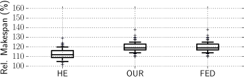
Figure 5: Rel.makespan for $100$ DAGs generated with parallelism $8$, connection probability $20\%$ on $2$ processors.

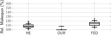
Figure 6: Rel.makespan for $100$ DAGs generated with parallelism $4$, connection probability $80\%$ on $8$ processors.

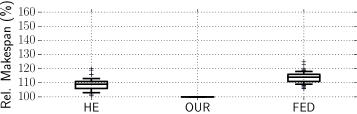
Figure 7: Rel.makespan for $100$ DAGs generated with parallelism $8$, connection probability $80\%$ on $16$ processors.

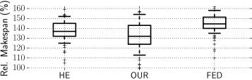
Figure 8: Rel.makespan for $100$ DAGs generated with parallelism $20$, connection probability $20\%$ on $16$ processors.

Observation (Low-Parallelism).  As shown in Figure 5 for the DAG set that was generated with the parameters parallelism $8$ and connection probability $20\%$ on $2$ processors, the analysis HE yields an average relative makespan of roughly $112\%$, whilst OUR approach degenerates to federated scheduling FED with roughly $119\%$. Due to the limited number of processors, our approach can not benefit from the inherent parallelism of the DAGs.

The other case, in which the parallel execution is limited by the number of processors, is shown in Figure 8. Here, the parallelism of $20$ is larger than the number of processors $16$, and OUR approach outperforms HE on average by as much as $5\%$. This case demonstrates that OUR approach can leverage the parallelism offered by the processors and the inherent parallelism of the DAGs to improve the response time.

Observation (High-Parallelism).  The largest performance improvements of OUR can be observed for highly parallel DAGs in combination with high processor availability. This case is shown in Figure 7 with parallelism of $8$ on $16$ processors and Figure 6 with parallelism of $4$ on $8$ processors. We observe that OUR approach not only outperforms HE in both cases, but that OUR approach even yields tight results for most evaluated DAGs.

VI-B Reservations Over-Provisioning Experiment

Waste Ratio. (%)	P=4	P=8	P=16
OUR-GANG min.	27.26	29.22	36.22
OUR-GANG max.	76.85	82.33	82.19
OUR-GANG average	53.76	59.26	61.97
OUR-GANG variance	87.06	74.42	62.14
OUR-ORD min.	13.79	21.89	36.87
OUR-ORD max.	76.64	81.77	82.07
OUR-ORD average	53.33	59.54	62.4
OUR-ORD variance	97.17	73.72	58.01

Table I: Minimal over-provisioning ratio for DAG sets with different degrees of parallelism $P$ on a system with infinite processors.

We compare OUR-GANG in Algorithm 2 and OUR-ORD in Algorithm 3 in terms of an waste ratio, i.e., the reserved service minus the total workload divided by the reserved service.

We generated 100 DAGs with $5$-$10$ for each of the following varying parameters: parallelism in $\left\{{4,8,16}\right\}$, connection probability in $\left\{{.1,.2,.3}\right\}$, deadline such that $vol(\pi_{*})<D<\min\left\{{\rho\cdot vol(\pi_{*}),C}\right\}$ for $\rho\in\left\{{1.2,1.4,1.6,1.8}\right\}$. We assume that a sufficient number of processors is available such that a reservation system can be found for every generated deadline. We then evaluated all generates sets with the same parallelism $P$ together and present the results in Table. I.

Observation.  The overall statistics of both reservation systems are quite similar for each level of parallelism. Especially, the average values only differ by $0.42\%$. For both, the waste ratio slightly increases with the amount of parallelism, resulting from the increased number of paths in a path collection (and thus at least a similar increase in the number of reservations) to exploit the parallelism and satisfy deadline constraints.

VI-C Reservations Improvement Experiment

Lastly, we compare our ordinary reservation system to the state-of-the-art hierarchical DAG scheduling approach proposed by Ueter et al. [33]. Recall that OUR-ORD is a generalization of their approach. That is, OUR-ORD, as generated by Algorithm 3, always has a higher resource efficiency, since a solution of Ueter et al. [33] is identical to our approach if $n=1$. However, to what extend resources in terms of the number of reservations and the overall service can be saved is not clear beforehand and thus subject to our second experiment. We use the same setup as described in Section VI-B and evaluate the reservation system as generated by Ueter et al. [33] referred to as UET against OUR-ORD with respect to the overall reserved service and the number of parallel reservations for DAGs with parallelism $P\in\left\{{4,8,16}\right\}$.

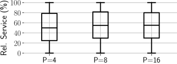
Figure 9: Reserved service of OUR-ORD normalized to UET for $100$ DAGs generated with parallelism $P\in\left\{{4,8,16}\right\}$.

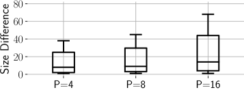
Figure 10: Absolute difference of the number of reservations of UET minus OUR-ORD for parallelism $P\in\left\{{4,8,16}\right\}$.

Size Difference	P=4	P=8	P=16
min.	1	1	1
max.	839	2035	3489
average	30.42	48.57	64.72
variance	5404.84	21760.85	43247.11

Table II: Statistics of the absolute reservation size differences for different degrees of parallelism $P$.

Observation (Service).  Figure 9 shows that the reserved service of OUR-ORD saves roughly $50\%$ on average for each level of parallelism, while the improvements are larger for smaller parallelism.

Observation (Size).  In Figure 10 and Table II, the results for the absolute differences in the reservation sizes, i.e., UET minus OUR-ORD, is shown. Table II shows that OUR-ORD can significantly decrease the number of required parallel reservations to meet deadline constraints by roughly $30,\leavevmode\nobreak\ 49,$ and $65$ reservations. Interestingly, the average difference is relatively stable compared to the range and variance for increasing degree of parallelism. This demonstrates that our approach can improve UET to be applicable for highly parallel DAG tasks with tight deadline constraints.

VII Related Work

Real-time aware scheduling of parallel task systems has been extensively studied for a variety of different proposed task models. Goosens et al. [16] have provided a classification of parallel task with real-time constraints.

Early work on parallel task models focused on synchronous parallel task models, e.g., [25, 29, 7]. Synchronous parallel task models extend the fork-join model [8] in such a way that they allow different numbers of subtasks in each (synchronized) segment where the number of subtasks can exceed the number of processors.

A prominent parallel task model that has been subject to many recent scheduling and analysis efforts, is the directed-acyclic graph (DAG) task model. The DAG models subtask-level parallelism by acyclic precedence constraints for a set of subtasks. This parallel model has been shown to correspond to models available in parallel computing APIs such as OpenMP by Melani et al. [30], Sun et al. [32], or Serrano et al. [31]. The parallel DAG task model has been studied for global [4, 27, 6] and partitioned scheduling [15, 5, 3, 14].

The proposed scheduling algorithms and analyses in the literature can be categorized into decompositional and non-decompositional. In the former, the parallel task model is decomposed into a set of sequential task models, which is scheduled and analyzed in their stead, e.g., [21]. Non-decompositional approaches consider the peculiarities of the parallel task models, e.g., [24, 33, 1, 27, 12, 4].

A prominent decomposition based approach is federated scheduling by Li et al. [24] that avoids inter-task interference for parallel tasks. It has been extended in, e.g., [22, 20, 11, 33, 1, 2]. In the original federated scheduling approach, the set of DAG tasks is partitioned into tasks that can be executed sequentially on a single processor and tasks that need to execute in parallel to finish before their respective deadlines.

VIII Conclusion and Future Work

We present the parallel path progression concept that allows to improve the self-interference analysis by explicitly considering the parallel execution of paths in the DAG. We propose a sustainable scheduling algorithm and analysis that is extended by virtue of hierarchical scheduling for gang-based and ordinary reservation systems for sporadic arbitrary-deadline DAG tasks. We designed an approximation algorithm for the $n$-path collection and proved that the then resulting makespan in our parallel path progression scheduling algorithm yields upper-bounds with respect to an optimal solution. For these reservations, we provide heuristic algorithms that provision reservation systems with respect to the service they require. We evaluated our approach using synthetically generated DAG task sets and demonstrated that our approach can improve the state-of-the art in high-parallelism scenarios while demonstrating reasonable performance for low-parallelism scenarios. In future work, we plan to improve the active idling issues of the proposed reservation systems by considering self-suspension behaviour for the reservation systems.

References

- [1] S. Baruah. The federated scheduling of constrained-deadline sporadic DAG task systems. In Proceedings of the Design, Automation & Test in Europe Conference & Exhibition, DATE, pages 1323–1328, 2015.
- [2] S. Baruah. Federated scheduling of sporadic DAG task systems. In IEEE International Parallel and Distributed Processing Symposium, IPDPS, pages 179–186, 2015.
- [3] S. Ben-Amor, L. Cucu-Crosjean, and D. Maxim. Worst-case Response Time Analysis for Partitioned Fixed-Priority DAG tasks on identical processors. In IEEE International Conference on Emerging Technologies and Factory Automation (ETFA), pages 1423–1426, 2019.
- [4] V. Bonifaci, A. Marchetti-Spaccamela, S. Stiller, and A. Wiese. Feasibility analysis in the sporadic dag task model. In ECRTS, pages 225–233, 2013.
- [5] D. Casini, A. Biondi, G. Nelissen, and G. Buttazzo. Partitioned Fixed-Priority Scheduling of Parallel Tasks Without Preemptions. In IEEE Real-Time Systems Symposium (RTSS), pages 421–433, 2018.
- [6] J.-J. Chen and K. Agrawal. Capacity augmentation bounds for parallel dag tasks under G-EDF and G-RM. Technical Report 845, Faculty for Informatik at TU Dortmund, 2014.
- [7] H. S. Chwa, J. Lee, K. Phan, A. Easwaran, and I. Shin. Global EDF Schedulability Analysis for Synchronous Parallel Tasks on Multicore Platforms. In Euromicro Conference on Real-Time Systems, ECRTS, pages 25–34, 2013.
- [8] M. E. Conway. A Multiprocessor System Design. In Proceedings of the November 12-14, 1963, Fall Joint Computer Conference, AFIPS ’63 (Fall), page 139–146. Association for Computing Machinery, 1963.
- [9] R. W. Deming. Independence numbers of graphs-an extension of the koenig-egervary theorem. Discrete Mathematics, 27(1):23–33, 1979.
- [10] R. P. Dilworth. A Decomposition Theorem for Partially Ordered Sets, pages 7–12. Birkhäuser Boston, Boston, MA, 1990.
- [11] S. Dinh, C. Gill, and K. Agrawal. Efficient deterministic federated scheduling for parallel real-time tasks. In 2020 IEEE 26th International Conference on Embedded and Real-Time Computing Systems and Applications (RTCSA), pages 1–10, 2020.
- [12] Z. Dong and C. Liu. Work-in-progress: New analysis techniques for supporting hard real-time sporadic dag task systems on multiprocessors. In 2018 IEEE Real-Time Systems Symposium (RTSS), pages 151–154, 2018.
- [13] D. G. Feitelson and L. Rudolph. Gang scheduling performance benefits for fine-grain synchronization. Journal of Parallel and Distributed Computing, 16:306–318, 1992.
- [14] J. Fonseca, G. Nelissen, and V. Nélis. Improved Response Time Analysis of Sporadic DAG Tasks for Global FP Scheduling. In Proceedings of the 25th International Conference on Real-Time Networks and Systems, pages 28–37, 2017.
- [15] J. C. Fonseca, G. Nelissen, V. Nélis, and L. M. Pinho. Response time analysis of sporadic DAG tasks under partitioned scheduling. In 11th IEEE Symposium on Industrial Embedded Systems, SIES, pages 290–299, 2016.
- [16] J. Goossens and V. Berten. Gang FTP scheduling of periodic and parallel rigid real-time tasks. CoRR, abs/1006.2617, 2010.
- [17] Q. He, x. jiang, N. Guan, and Z. Guo. Intra-task priority assignment in real-time scheduling of dag tasks on multi-cores. IEEE Transactions on Parallel and Distributed Systems, 30(10):2283–2295, 2019.
- [18] Q. He, M. Lv, and N. Guan. Response time bounds for DAG tasks with arbitrary intra-task priority assignment. In ECRTS, volume 196, pages 8:1–8:21, 2021.
- [19] M. A. Jette. Performance characteristics of gang scheduling in multiprogrammed environments. In Proceedings of the 1997 ACM/IEEE Conference on Supercomputing, SC ’97, 1997.
- [20] X. Jiang, N. Guan, H. Liang, Y. Tang, L. Qiao, and W. Yi. Virtually-federated scheduling of parallel real-time tasks. In 2021 IEEE Real-Time Systems Symposium (RTSS), pages 482–494, 2021.
- [21] X. Jiang, N. Guan, X. Long, and H. Wan. Decomposition-based real-time scheduling of parallel tasks on multicores platforms. IEEE Transactions on Computer-Aided Design of Integrated Circuits and Systems, 39, 2020.
- [22] X. Jiang, N. Guan, X. Long, and W. Yi. Semi-federated scheduling of parallel real-time tasks on multiprocessors. In Proceedings of the 38nd IEEE Real-Time Systems Symposium, RTSS, 2017.
- [23] K. Lakshmanan, S. Kato, and R. R. Rajkumar. Scheduling parallel real-time tasks on multi-core processors. In Proceedings of the 31st IEEE Real-Time Systems Symposium, pages 259–268, 2010.
- [24] J. Li, J.-J. Chen, K. Agrawal, C. Lu, C. D. Gill, and A. Saifullah. Analysis of federated and global scheduling for parallel real-time tasks. In 26th Euromicro Conference on Real-Time Systems, ECRTS, pages 85–96, 2014.
- [25] C. Maia, M. Bertogna, L. Nogueira, and L. M. Pinho. Response-Time Analysis of Synchronous Parallel Tasks in Multiprocessor Systems. In M. Jan, B. B. Hedia, J. Goossens, and C. Maiza, editors, 22nd International Conference on Real-Time Networks and Systems, RTNS, page 3, 2014.
- [26] A. Melani, M. Bertogna, V. Bonifaci, A. Marchetti-Spaccamela, and G. C. Buttazzo. Response-Time Analysis of Conditional DAG Tasks in Multiprocessor Systems. In Proceedings of the 2015 27th Euromicro Conference on Real-Time Systems, 2015.
- [27] M. Nasri, G. Nelissen, and B. B. Brandenburg. Response-Time Analysis of Limited-Preemptive Parallel DAG Tasks Under Global Scheduling. In 31st Euromicro Conference on Real-Time Systems (ECRTS), pages 21:1–21:23, 2019.
- [28] G. L. Nemhauser, L. A. Wolsey, and M. L. Fisher. An analysis of approximations for maximizing submodular set functions—i. Mathematical Programming, 14:265–294, 1978.
- [29] A. Saifullah, K. Agrawal, C. Lu, and C. Gill. Multi-Core Real-Time Scheduling for Generalized Parallel Task Models. In Proceedings of the 32nd IEEE Real-Time Systems Symposium, pages 217–226, 2011.
- [30] M. A. Serrano, A. Melani, R. Vargas, A. Marongiu, M. Bertogna, and E. Quiñones. Timing characterization of OpenMP4 tasking model. In International Conference on Compilers, Architecture and Synthesis for Embedded Systems, CASES, pages 157–166, 2015.
- [31] M. A. Serrano, S. Royuela, and E. Quiñones. Towards an openmp specification for critical real-time systems. In B. R. de Supinski, P. Valero-Lara, X. Martorell, S. Mateo Bellido, and J. Labarta, editors, Evolving OpenMP for Evolving Architectures, pages 143–159, Cham, 2018. Springer International Publishing.
- [32] J. Sun, N. Guan, Y. Wang, Q. He, and W. Yi. Real-time scheduling and analysis of OpenMP task systems with tied tasks. In IEEE Real-Time Systems Symposium, RTSS, pages 92–103, 2017.
- [33] N. Ueter, G. von der Brüggen, J.-J. Chen, J. Li, and K. Agrawal. Reservation-based federated scheduling for parallel real-time tasks. In IEEE Real-Time Systems Symposium (RTSS), pages 482–494, 2018.
- [34] S. Wasly and R. Pellizzoni. Bundled scheduling of parallel real-time tasks. In RTAS, pages 130–142. IEEE, 2019.
- [35] S. Zhao, X. Dai, I. Bate, A. Burns, and W. Chang. DAG scheduling and analysis on multiprocessor systems: Exploitation of parallelism and dependency. In RTSS, pages 128–140. IEEE, 2020.