What Impulse Response Do Instrumental Variables Identify?

Macro shocks are often composites, yet overlooked in the impulse response analysis. When an instrumental variable (IV) is used to identify a composite shock, it violates the common IV exclusion restriction. We show that the Local Projection-IV estimand is represented as a weighted average of component-wise impulse responses but with possibly negative weights, which occur when the IV and shock components have opposite correlations. We further develop alternative (set-) identification strategies for the LP-IV based on sign restrictions or additional granular information. Our applications confirm the composite nature of monetary policy shocks and reveal a non-defense spending multiplier exceeding one.

Keywords: local projection, structural vector moving average, instrumental variables, sectoral heterogeneity, impulse response, government spending multiplier, sign restrictions, set identification

1   Introduction

In contemporary applied macroeconometrics literature, instrumental variables (IVs) are frequently employed as a crucial source of external variation for identifying impulse response functions to macroeconomic shocks relevant to policy analysis. Two commonly used approaches for utilizing IVs are the IV estimation in the local projection (LP-IV) framework and the estimation of extended structural vector autoregressions (SVARs), wherein the external IVs are included in the system. This approach includes the proxy SVAR.

While the interpretation of estimates in the extended SVAR is more straightforward due to its specification of a complete system, the same cannot be said for the LP-IV approach, since an instrumental variable model is inherently partial. The econometric literature has devoted substantial effort to build a general framework, under which one can properly interpret IV estimands, as evidenced by the development of methods such as the local average treatment effect (LATE) in Imbens and Angrist (1994); Bartik instruments in Goldsmith-Pinkham, Sorkin, and Swift (2020), Borusyak, Hull, and Jaravel (2022), and Adao, Kolesár, and Morales (2019); two-stage least squares in Mogstad, Torgovitsky, and Walters (2021), and others. A common identification assumption for the LP-IV estimand is the so-called IV exclusion restriction as in Plagborg-Møller and Wolf’s (2021) Eq. (16) or Stock and Watson’s (2018) Condition LP-IV^⟂, in which the IV is correlated with only a single structural shock. It is too restrictive since it even excludes various proxy SVAR models.

To address this issue, we employ a potentially non-invertible vector moving average (SVMA) model and allow for the IVs to be correlated with multiple structural shocks. Specifically, the SVMA model recognizes that a monetary or fiscal policy shock, with which IVs are associated, may not be homogeneous but composite in nature. For instance, a government spending shock can be a combination of sectoral spending shocks with varying relative magnitudes, while a monetary policy surprise comprises expectations about policy tightening in different time horizons or a pure monetary shock along with the central bank’s assessment of economic conditions. Although the composite nature of macro shocks has been well understood in macroeconomics literature, the current LP-IV literature does not adequately account for it (e.g., Stock and Watson (2018), Plagborg-Møller and Wolf (2021, 2022)). Therefore, this paper aims to bridge this gap by considering the composite nature of macro shocks within the LP-IV framework.

We show that the impulse response identified by the LP-IV method can be expressed as a weighted sum of impulse responses to the individual components of the composite shock, with the weights determined by the correlation between the instrument and each component shock. Since the correlation is not restricted to be non-negative, this implies that the LP-IV estimand does not necessarily identify any informative quantity as to the impulse response we aim to recover.

To fix ideas, suppose that we are to estimate the response of GDP at horizon $h$ to a unit change in government spending. Since the observed changes in government spending is unlikely exogenous, an IV is required to identify the government spending multiplier. Ramey and Zubairy (2018) use the narrative military news as the instrument to provide exogenous variation in government spending. The cumulative government spending multiplier is estimated by LP-IV. The LP-IV estimand (the population counterpart of the estimator) is given by

$$\beta_{h}=\frac{\text{cov}\left(\sum_{j=0}^{h}y_{t+j},z_{t}\right)}{\text{cov}\left(\sum_{j=0}^{h}x_{t+j},z_{t}\right)},$$ (1)

where $y_{t}$ is the GDP, $x_{t}$ is the government spending variable, and $z_{t}$ is the military news shock. Since government spending consists of defense and non-defense spending, we find that

$$\beta_{h}=w_{\text{defense}}\times\theta_{h,\text{defense}}+w_{\text{non-defense}}\times\theta_{h,\text{non-defense}},$$ (2)

where $\theta_{h,\text{defense}}$ and $\theta_{h,\text{non-defense}}$ are the defense and non-defense spending multipliers, respectively, and $w$ is the weight whose sign depends on the correlation of the military news shock and the sectoral spending shock. $\beta_{h}$ has a causal interpretation only if $w$ is between zero and one. It may be interpreted as the aggregate spending multiplier when $w$ is the proportion of sectoral spending. However, in our replication of Ramey and Zubairy (2018) in Section 5, we find that for $h=18$ (eighteen quarters) the LP-IV estimator is decomposed as

$$\begin{array}[]{ccccccccc}\widehat{\beta}_{h}&=&\widehat{w}_{\text{defense}}&\times&\widehat{\theta}_{h,\text{defense}}&+&\widehat{w}_{\text{non-defense}}&\times&\widehat{\theta}_{h,\text{non-defense}}.\\ 0.37&&1.87&&0.68&&-0.87&&1.02\\ \end{array}$$ (3)

Due to the negative weight, the estimated government spending multipler is much smaller than either the defense or non-defense spending multiplier. This would lead to an inaccurate empirical conclusion for researchers and policy makers even when the instrument and the estimation procedure are legitimate and valid.

The issue arising from the negative weights has received much attention recently in the microeconometrics literature. For instance, de Chaisemartin and D’Haultfoeuill (2020) show that the regression coefficient in the two-way fixed effects model can be expressed as a weighted sum of the average treatment effects where the weight can be negative due to different timing of treatment receipts across units. Mogstad, Torgovitsky, and Walters (2021) show that the two-stage least squares estimand using multiple instruments may lose a causal interpretation due to negative weights assigned to some subpopulation under general treatment effect heterogeneity.

Our finding that the impulse response identified by an instrument is an informative quantity only if the weights are nonnegative has important practical implications. Researchers should carefully discuss potential shock components in the macro shock of interest and their correlation with the instrument. Depending on the sign of the correlations, some instruments provide valid structural interpretations while others do not, despite all being valid in the conventional IV framework.

What if your instrument shows negative correlation with specific component shocks? Fortunately, it still holds value. By utilizing the two identification strategies we propose below, one can infer on the impulse responses to the individual components of the component shock.

Our first identification strategy is sign restrictions, which uses the signs of the weights to obtain bounds for the identified set of componentwise impulse responses. Sign restrictions are commonly used in the SVAR literature (e.g. Uhlig, 2005) and suggested by Plagborg-Møller and Wolf (2021) in the LP framework. Our approach differs in that we place restrictions on the weight rather than the structural impulse response. Since the sign of the weight is determined by the sign of the correlation between the instrument and the individual component shock, our sign restrictions are easier to justify. Additionally, our strategy requires no additional computation since LP-IV estimates are directly used as bound estimates, unlike other approaches that often require extensive computation or simulation. Lastly, our approach easily accommodates sign restrictions with multiple instruments as a tighter identified set can be obtained by simply intersecting the bounds.

To illustrate the first identification strategy, in Section 4 we revisit Jarociński and Karadi (2020) where the central bank information shock is purged from the central bank’s monetary policy announcement to identify the pure monetary policy shock. By using high-frequency financial market surprises as the instruments, we impose sign restrictions between the monetary policy shock and the instruments in the LP-IV model to obtain the identified set for the pure monetary policy shock. We note that the analysis of Jarociński and Karadi (2020) is based on the Bayesian SVAR, which is the standard approach to use sign restrictions in the VAR model (e.g., Uhlig, 2005). Moon and Schorfheide (2012) and Granziera, Moon, and Schorfheide (2018) have analyzed the asymptotic difference between the Bayesian and frequentist approaches to the set estimation and shown that the Bayesian highest posterior density sets excludes parts of the estimated identified sets while the frequentist confidence sets extend beyond the boundaries of the estimated identified set.

Our second identification strategy for componentwise impulse responses is to use more granular level data to identify the weights. For example, quarterly data on defense and non-defense spending in the US after the WWII are available and we can use these variables to identify the weights for the defense and non-defense spending multipliers. In addition, when the number of available instruments is at least as many as the number of components in the composite shock, the componentwise impulse responses can be point identified. In Section 5 we estimate the defense and non-defense spending multipliers using the sectoral spending data and two instruments, the military news shock of Ramey and Zubairy (2018) and the current defense spending shock of Blanchard and Perotti (2002).

We would like to highlight that although our main results are based on the impulse responses estimated by LP-IV, our findings have broader implications. Plagborg-Møller and Wolf (2021) have demonstrated that LP-IV and SVAR with the instrument ordered first in the triangular system, estimate the same impulse responses asymptotically. While their analysis did not include composite macro shocks, we believe that our findings could similarly extend to impulse responses estimated by SVAR with instruments. We focus on the LP-IV due to its simplicity in estimation and structural interpretation (Stock and Watson, 2018). Moreover, since the LP specification is more flexible than the SVAR specification, the LP-IV estimator may be more robust to misspecification of the true data generating process (Nakamura and Steinsson, 2018).

Our paper is related to program evaluations under treatment effect heterogeneity. In their influential paper, Imbens and Angrist (1994) demonstrated that a valid IV can only identify the LATE in the potential outcomes framework. Since it is natural to consider a macroeconomic shock as the treatment and the impulse response as the treatment effect, our result can be seen as an extension of LATE to impulse response analysis. However, there are several important differences between our framework and the potential outcomes framework. First, unlike the potential outcomes framework, where the set of treatments is a singleton or finite, we define the composition of the macroeconomic shock as the treatment, which is naturally a continuum. For example, a one-unit exogenous change in government spending may consist entirely of defense spending or some combination of defense and non-defense spending. Second, unlike the potential outcomes framework, where everyone gets homogeneous treatment but their individual treatment effects are heterogeneous, the composition of a macro shock provides heterogeneous treatment, but the response of the macro variables is homogeneous conditional on the composition. We discuss the similarities and differences in the identified structural parameters and identifying conditions between our framework and the potential outcomes framework in detail in Section 2.3.

Lastly, we provide a brief literature review. There is a significant body of work that uses IVs in macroeconometrics. Some notable examples include Stock and Watson (2012), Mertens and Ravn (2013), Gertler and Karadi (2015), and Jarociński and Karadi (2020), who employ IVs for identification in SVAR models. The LP method were introduced by Jordà (2005), and LP-IV have been used in several studies, such as Jordà, Schularick, and Taylor (2015, 2020), Stock and Watson (2018), and Ramey and Zubairy (2018).

Our paper is organized as follows. Section 2 introduces the underlying structural model and shows what the LP-IV identifies. We develop identification strategies for the componentwise impulse responses in Section 3, employing sign restrictions or leveraging granular data. The empirical applications concerning the analysis of monetary policy and the fiscal multiplier are given in Section 4 and 5. Section 6 concludes. The proofs of Propositions, supplementary inference procedures, and their theoretical justifications are collected in the Appendix.

2   Model and Identification

We adopt the non-invertible structural vector moving average (SVMA) model and investigate identifiability of the structural parameters in the model that determine the impulse responses and policy multipliers. SVMA is useful due to its flexible nature such that it allows for a larger number of structural shocks than the observable endogenous variables.

2.1 Structural Vector Moving Average

Let $\bm{Y}_{t}$ be an $n\times 1$ vector of observed endogenous variables and let $\bm{\varepsilon}_{t}$ be an $m\times 1$ vector of unobserved structural shocks. The endogenous variables $\bm{Y}_{t}$ is written as a linear combination of current and past $\bm{\varepsilon}_{t}$’s:

$$\bm{Y}_{t}=\bm{\Theta}(L)\bm{\varepsilon}_{t}$$ (4)

where $L$ is the lag operator, $\bm{\Theta}(L)=\bm{\Theta}_{0}+\bm{\Theta}_{1}L+\bm{\Theta}_{2}L^{2}+\cdots$, and $\bm{\Theta}_{h}$ for $h=0,1,2,...$ is an $n\times m$ matrix of impulse response coefficients. We assume that $E[\bm{\varepsilon}_{t}]=0$, $E[\bm{\varepsilon}_{t}\bm{\varepsilon}_{t}^{\prime}]>0$, and the shocks are mutually uncorrelated. A word on notation: we reserve the index ‘$s$’ to indicate an element in the system (4), e.g., $\varepsilon_{s,t}$ then denotes the $s$-th element of $\bm{\varepsilon}_{t}$.

Let $y_{t}$ be the last element of $\bm{Y}_{t}$ without loss of generality. We define the impulse response of $y_{t}$ at horizon $h$ to the shock $\varepsilon_{s,t}$ as

$$\theta_{h,ys}\equiv E[y_{t+h}|\varepsilon_{s,t}=1]-E[y_{t+h}|\varepsilon_{s,t}=0].$$

Here we are slightly abusing notation by letting $\theta_{h,ys}$ be the $(n,s)$-th element of $\bm{\Theta}_{h}$. This is to emphasize that $y_{t}$ is the main variable of interest.

The researcher is interested in the impulse response of $y_{t}$ at horizon $h$ to a macroeconomic shock $\xi_{t}$, $\theta_{h,y\xi}\equiv E[y_{t+h}|\xi_{t}=1]-E[y_{t+h}|\xi_{t}=0]$. The shock $\xi_{t}$ may not be an element of $\bm{\varepsilon}_{t}$ but a composite shock that consists of multiple structural shocks $\varepsilon_{s,t}$ for $s\in\mathcal{S}_{\xi}\subseteq\{1,2,...,m\}$. Without loss of generality, let the elements of $\mathcal{S}_{\xi}$ be the first $S$ elements of $\bm{\varepsilon}_{t}$, so that we can write

$$\xi_{t}=\sum_{s=1}^{S}\varepsilon_{s,t}.$$

Conventionally in the literature, the shock $\xi_{t}$ has been often treated as a single unit as if it consisted of identical structural shocks.

Quite a few papers document that a policy shock is a composite shock consisting of either more disaggregate policy shocks or shocks with distinct, often opposite nature and impact. For fiscal policy shocks, Auerbach and Gorodnichenko (2012) show that more disaggregate spending behave differently relative to an aggregate fiscal policy shock. Cox, Müller, Pasten, Schoenle, Weber (2020) and Bouakez, Rachedi and Santoro (2020) note that the composition of aggregate government spending heavily affects the aggregate spending multiplier and discuss sector-specific government spending multipliers. Meanwhile, monetary policy shocks, unlike government spending which can be easily categorized by sectors, are categorized by its impact to the economy. For instance, Jarociński and Karadi (2020) decompose a monetary policy announcement into a pure monetary policy shock and an information shock. Kaminska, Mumtaz, and S̆ustek (2021), on the other hand, decompose it to three components: shocks to the short term policy rate (action shocks), shocks due to communication about future economic conditions or policy intentions (path shocks), and shocks to risk premia due to the effect of communication on uncertainty (premia shocks).

When researchers consider the impulse response of $y_{t+h}$ to a composite shock $\xi_{t}$ (i.e., $\theta_{h,y\xi}$), what they wish to identify is some weighted average of $\theta_{h,ys}$ for $s=1,2,...,S$. To illustrate this, assume that the shocks are discrete random variables. Further assuming the convention that $E[y_{t+h}|\xi_{t}=0]$ corresponds to $\bm{e}_{t}\equiv(\varepsilon_{1,t},\varepsilon_{2,t},\cdots,\varepsilon_{S,t})^{\prime}=\bm{0}$, we can write

$$\theta_{h,y\xi}= \sum_{\bm{a}\in\{\xi_{t}=1\}}\frac{P(\bm{e}_{t}=\bm{a})}{P(\{\xi_{t}=1\})}\left(E[y_{t+h}|\bm{e}_{t}=\bm{a}]-E[y_{t+h}|\bm{e}_{t}=\bm{0}]\right)$$ (5)

$$= \sum_{\bm{a}\in\{\xi_{t}=1\}}\frac{P(\bm{e}_{t}=\bm{a})}{P(\{\xi_{t}=1\})}\bm{a}^{\prime}\bm{\theta}_{h,y}$$

$$= E[\bm{e}_{t}|\xi_{t}=1]^{\prime}\bm{\theta}_{h,y}$$ (6)

where $\bm{a}$ is an $S\times 1$ non-random vector, $\{\xi_{t}=1\}$ is a collection of realizations of $\bm{e}_{t}$ such that $\xi_{t}=1$, and $\bm{\theta}_{h,y}=(\theta_{h,y1},\theta_{h,ys},...,\theta_{h,yS})^{\prime}$. Thus, $\theta_{h,y\xi}$ is a weighted average of componentwise impulse responses and the weights are the mean of $\varepsilon_{s,t}$ conditional on $\xi_{t}=1$, which are non-negative for a large class of reasonable distributions of $\bm{e}_{t}$. For example, if we assume $\varepsilon_{s,t}$ for $s=1,...,S$ are i.i.d., then $E[\varepsilon_{s,t}|\xi_{t}=1]=1/S$ and (6) becomes the equal-weighted average.

However, $\xi_{t}$ is typically unobserved and its scale is indeterminate. A common solution to this problem is to measure the magnitude of $\xi_{t}$ by means of an observable endogenous variable $x_{t}$ and then to use an instrument $z_{t}$ correlated with $x_{t}$ to get external variation. As a result, the response of $y_{t+h}$ to $z_{t}$ relative to the response of $x_{t}$ to $z_{t}$ can be interpreted as the average response of $y_{t+h}$ to $\xi_{t}$ of a magnitude that corresponds to a unit change in $x_{t}$. Stock and Watson (2018) provide an example that the causal effect of GDP growth ($y_{t}$) to a monetary policy shock ($\xi_{t}$) can be identified by the ratio of the impulse responses of GDP growth and the federal fund rate ($x_{t}$) to a monetary policy announcement ($z_{t}$). Ramey and Zubairy (2018) calculate the government spending multiplier as a ratio of the impulse responses of GDP ($y_{t}$) and total government spending ($x_{t}$) to the military news shock ($z_{t}$).

Let $x_{t}$ be the first element of $\bm{Y}_{t}$ without loss of generality. Similar to $y_{t}$, we define the impulse response of $x_{t}$ at horizon $h$ to the shock $\varepsilon_{s,t}$ as $\theta_{h,xs}$ by slightly abusing notation. To fix the scale of $\varepsilon_{s,t}$, we assume that $\theta_{0,xs}=1$ for all $s=1,2,...,S$, which is referred to as the unit effect normalization in the literature (Stock and Watson, 2018). In the government spending shock example, the unit effect normalization means a unit change in a sectoral spending shock changes the total spending by one unit.

2.2 Local Projections with Instrumental Variables

Let $z_{t}$ be an instrument that satisfies the following assumptions.

Assumption 1.

1. $E[z_{t}\xi_{t}]\neq 0$ (relevance)

2. $E[z_{t}\varepsilon_{s,t}]=0$ for all $s=S+1,S+2,...,m$ (contemporaneous exogeneity)

3. $E[z_{t}\bm{\varepsilon}_{t+j}]=0$ for $j\neq 0$ (lead-lag exogeneity)

Define $E[z_{t}\varepsilon_{s,t}]=\alpha_{s}$. Assumption 1(i) implies that $\alpha_{s}\neq 0$ for some $s=1,2,...,S$. Assumption 1 is an extension of Condition LP-IV of Stock and Watson (2018) allowing that more than one structural shocks are correlated with the instrument $z_{t}$ and the correlations are heterogeneous across the shocks.

For illustration purposes, let us assume that the instrument $z_{t}$ is binary and $0<P(z_{t}=1)<1$. Write $P_{z}=P(z_{t}=1)$. Also assume that $S=2$ so that $\xi_{t}$ is the sum of two structural shocks, $\varepsilon_{1,t}$ and $\varepsilon_{2,t}$. A direct IV estimator of the impulse response is the LP-IV estimator, whose population version is given by

$$\beta_{h}\equiv\frac{E[y_{t+h}|z_{t}=1]-E[y_{t+h}|z_{t}=0]}{E[x_{t}|z_{t}=1]-E[x_{t}|z_{t}=0]}.$$

The LP-IV estimand $\beta_{h}$ is the ratio of two IV-impulse responses and it takes the form of the Wald estimand in the microeconometrics literature. Since $y_{t+h}$ is a linear combination of $\bm{\varepsilon}_{t+h-j}$ for $j=0,1,2,...$ by (4), the numerator of $\beta_{h}$ can be written as

$$E[y_{t+h}|z_{t}=1]-E[y_{t+h}|z_{t}=0]=\sum_{s=1}^{2}(E[\varepsilon_{s,t}|z_{t}=1]-E[\varepsilon_{s,t}|z_{t}=0])\theta_{h,ys}=\frac{\alpha_{1}\theta_{h,y1}+\alpha_{2}\theta_{h,y2}}{P_{z}(1-P_{z})}$$

under Assumption 1. Likewise,

$$E[x_{t}|z_{t}=1]-E[x_{t}|z_{t}=0]=\sum_{s=1}^{2}(E[\varepsilon_{s,t}|z_{t}=1]-E[\varepsilon_{s,t}|z_{t}=0])\theta_{0,xs}=\frac{\alpha_{1}+\alpha_{2}}{P_{z}(1-P_{z})},$$

under the unit effect normalization. As a result, $\beta_{h}$ can be written as

$$\beta_{h}=\frac{\alpha_{1}}{\alpha_{1}+\alpha_{2}}\theta_{h,y1}+\frac{\alpha_{2}}{\alpha_{1}+\alpha_{2}}\theta_{h,y2},$$ (7)

which is an affine combination of the impulse responses $\theta_{h,y1}$ and $\theta_{h,y2}$. Equation (7) demonstrates that without a restriction on $\alpha_{s}$ we would not be able to interpret $\beta_{h}$ as a structural parameter. To see this, suppose that $\theta_{h,y1}=1$ and $\theta_{h,y2}=2$ so the impulse responses are both positive. However, if $\alpha_{1}=2$ and $\alpha_{2}=-1$, we have $\beta_{h}=0$. This can happen if the instrument $z_{t}$ is correlated with the two structural shocks, $\varepsilon_{1,t}$ and $\varepsilon_{2,t}$, in the opposite direction. Without a restriction on $\alpha_{s}$, $\beta_{h}$ can be any real number.

We do not have this problem when the composite shock consists of one structural shock ($S=1$). In this case, $\xi_{t}=\varepsilon_{s,t}$ and the LP-IV estimand $\beta_{h}=\theta_{h,ys}$. This special case corresponds to the standard LP-IV setup of Stock and Watson (2018) and Plagborg-Møller and Wolf (2021).

The following proposition establishes that the LP-IV estimand with a general non-binary IV is an affine combination of the structural impulse responses. The proof is in Appendix A.

Proposition 1.

If random variables $y_{t}$ and $x_{t}$ are elements of $\bm{Y}_{t}$ generated according to (4) and a random variable $z_{t}$ satisfies Assumption 1, then for $h=0,1,2,...$,

$$\beta_{h}\equiv\frac{Cov(y_{t+h},z_{t})}{Cov(x_{t},z_{t})}=\sum_{s=1}^{S}w_{s}\theta_{h,ys},$$ (8)

under the unit effect normalization, where

$$w_{s}=\frac{\alpha_{s}}{\sum_{s^{\prime}=1}^{S}\alpha_{s^{\prime}}}.$$

When there is only one component in $\xi_{t}$ (i.e., $S=1$), (8) simplifies to Equation (8) of Stock and Watson (2018). Thus, Proposition 1 generalizes the previous identification result to cases when the instrument is correlated with multiple structural shocks in the SVMA model (4).

Proposition 1 is not a complete identification result because the RHS of (8) is not a convex combination, i.e., a weighted average with non-negative weights, but an affine combination. To interpret $\beta_{h}$ as a meaningful average of the underlying structural impulse responses, we require the following assumption.

Assumption SS.

For all $s=1,2,...,S$, either $\alpha_{s}\geq 0$ or $\alpha_{s}\leq 0$. (same-sign)

Assumption SS restricts the way the instrument $z_{t}$ is correlated with the endogenous variable $x_{t}$ via the relevant structural shocks $\varepsilon_{s,t}$. Assumption SS is analogous to the monotonicity assumption for identification of LATE (Imbens and Angrist, 1994). We provide further discussion comparing the conditions and identification results in Section 2.3.

Since $E[\bm{Y}_{t}]=0$, $\bm{Y}_{t}$ is typically specified in differences or changes, but researchers may be interested in the level of $\bm{Y}_{t}$. The difference in the levels between $t$ and $t+h$ can be written as the cumulative changes over the $h$ periods: $\sum_{j=0}^{h}\bm{Y}_{t+j}$. Write $\widetilde{y}_{t+h}=\sum_{j=0}^{h}y_{t+j}$ and $\widetilde{x}_{t+h}=\sum_{j=0}^{h}x_{t+j}$. Define the cumulative impulse responses as $\widetilde{\theta}_{h,ys}=\sum_{j=0}^{h}\theta_{j,ys}$ and $\widetilde{\theta}_{h,xs}=\sum_{j=0}^{h}\theta_{j,xs}$, respectively.

Corollary 1.

If random variables $y_{t}$ and $x_{t}$ are elements of $\bm{Y}_{t}$ generated according to (4), a random variable $z_{t}$ satisfies Assumption 1, and $\widetilde{\theta}_{h,xs}\neq 0$ for all $s=1,2,...,S$, then for $h=0,1,2,...$,

$$\widetilde{\beta}_{h}\equiv\frac{Cov\left(\widetilde{y}_{t+h},z_{t}\right)}{Cov\left(\widetilde{x}_{t+h},z_{t}\right)}=\sum_{s=1}^{S}\left(\frac{\alpha_{s}\widetilde{\theta}_{h,xs}}{\sum_{s^{\prime}=1}^{S}\alpha_{s^{\prime}}\widetilde{\theta}_{h,xs^{\prime}}}\right)\frac{\widetilde{\theta}_{h,ys}}{\widetilde{\theta}_{h,xs}}.$$ (9)

Corollary 1 is relevant for identification and estimation of the cumulative impulse responses, such as the cumulative government spending multiplier using external instruments as in Ramey and Zubairy (2018). Their LP-IV estimand takes the form of the LHS of (9) after controlling for the lagged variables, where $y_{t}$ is the GDP, $x_{t}$ is government spending, $z_{t}$ is the military news shock, all relative to the trend GDP.

Assume that the government spending shock consists of defense ($s=1$) and non-defense ($s=2$) spending shocks: $\xi_{t}=\varepsilon_{1,t}$ + $\varepsilon_{2,t}$. For the LP-IV estimand to have structural interpretation, a version of Assumption SS is required to ensure non-negative weights. This would be that for $s=1,2$, either $\alpha_{s}\widetilde{\theta}_{h,xs}\geq 0$ or $\alpha_{s}\widetilde{\theta}_{h,xs}\leq 0$. We can check if the assumption is plausible. First, it is reasonable to assume that positive sectoral spending shocks have positive impacts on the cumulative government spending: $\widetilde{\theta}_{h,xs}>0$ for $s=1,2$. Next, it is reasonable to assume that the military news shock is positively correlated with the defense spending shock ($\alpha_{1}>0$). Thus, the weight for the non-defense spending multiplier would be non-negative if the military news shock is non-negatively correlated with the non-defense spending shock ($\alpha_{2}\geq 0$). If this is justified, then the estimand is a weighted average of the cumulative sectoral spending multiplier. On the other hand, if $\alpha_{2}<0$, the estimand may not provide meaningful information about the government spending multiplier because the estimand can be close to zero or even negative while the defense and non-defense spending multipliers are strictly greater than one. We find empirical evidence supporting $\alpha_{2}<0$ in Section 5.

2.3 Comparison with Other IV Estimands

2.3.1 Potential outcomes framework and LATE

Imbens and Angrist (1994) and Angrist, Imbens, and Rubin (1996) show that the local average treatment effect (LATE) is identified by an instrument under treatment effect heterogeneity. Let $Y_{i}$ be the observed outcome and $D_{i}$ be an indicator of treatment for individual $i$. Their analysis is based on the potential outcomes framework: the potential outcomes $Y_{i}(1)$ and $Y_{i}(0)$ are defined as the outcome with treatment ($D_{i}=1$) and without treatment ($D_{i}=0$), respectively. The observed outcome is written as $Y_{i}=Y_{i}(0)+(Y_{i}(1)-Y_{i}(0))D_{i}$. The individual treatment effect is $Y_{i}(1)-Y_{i}(0)$, which is assumed to be heterogeneous. Since the potential outcomes for an individual are not observed at the same time, the individual treatment effect is not identified. Therefore, the goal is to identify the average treatment effect (ATE), $E[Y_{i}(1)-Y_{i}(0)]$, or a version of ATE. Here, the treatment is homogeneous within the treated and non-treated groups, but the treatment effects are heterogeneous.

In comparison, the composite shock $\xi_{t}$ is the (unobserved) treatment. The ATE corresponds to the impulse response of $y_{t+h}$ to $\xi_{t}$: $E[y_{t+h}|\xi_{t}=1]-E[y_{t+h}|\xi_{t}=0]$, which is a weighted average of componentwise impulse responses as shown in (6). Unlike the ATE, heterogeneity arises in the composition of $\xi_{t}$, so that the treatment is heterogeneous. Since the componentwise impulse responses are assumed constant, the treatment effect of a particular composition in $\xi_{t}$ is homogeneous.

The IV provides exogenous variation in the endogenous variable in both cases. However, due to the different nature of the endogeneity (selection vs simultaneity), how the instrument provides identification of structural parameters in the two frameworks are different. This is illustrated in Figure 1.

Figure 1: Monotonicity and Same-Sign

First, consider a binary instrument $Z_{i}$ in the LATE case (left panel in Figure 1). $D_{i}$ is endogenous because it is not randomly assigned. For each value of $Z_{i}$, define the potential treatment status $D_{i}(1)$ and $D_{i}(0)$, which corresponds to $Z_{i}=1$ and $Z_{i}=0$, respectively. Angrist, Imbens, and Rubin (1996) define four subpopulations depending on the potential treatment status: always-takers ($D_{i}(1)=D_{i}(0)=1$), never-takers ($D_{i}(1)=D_{i}(0)=0$), compliers ($D_{i}(1)=1$, $D_{i}(0)=0$), and defiers ($D_{i}(1)=0$, $D_{i}(0)=1$). Imbens and Angrist (1994) show that the IV estimand identifies the ATE of the compliers (thus the local average), who would receive the treatment if $Z_{i}=1$ but not otherwise. Here, the key identification condition is the monotonicity condition (Condition 2 of Imbens and Angrist, 1994) that there is no defiers (who behave in the opposite way to the compliers) in the population. This is a restriction on the individual behavior, which should be justified carefully within the context.

Now consider our framework (right panel in Figure 1). Since $\xi_{t}$ is not observed and its scale is indeterminate, we need to measure the response of $y_{t+h}$ to $\xi_{t}$ relative to the response of another observable endogenous variable $x_{t}$ to $\xi_{t}$. $x_{t}$ is endogenous due to simultaneity because the shock $\xi_{t}$ affects $y_{t+h}$ and $x_{t}$ simultaneously. The LP-IV estimand has a structural interpretation only if the correlation between the instrument and the shock components in $\xi_{t}$ have the same sign. This same-sign condition (Assumption SS) plays an analogous role to the monotonicity condition as it restricts the average relationship between the instrument and the shocks.

There are a few papers using the potential outcomes framework in the time-series context. Angrist and Kuersteiner (2011) develop semiparametric tests for conditional independence, also known as the unconfoundedness condition. Analogous to the cross-sectional case, the potential outcomes with and without the treatment at time $t$ are not observed simultaneously and the time-specific treatment effects are heterogeneous. Their framework is different from ours because (i) the policy variable (treatment) is observed, (ii) the policy variable is independent of potential outcomes after conditioning on observables, and as a result, (iii) the role of IV is not discussed.

Rambachan and Shephard (2021) provide a more general potential outcomes framework allowing for unobserved treatment and the use of IV. Their IV identification result relies on a time-series version of the monotonicity condition. Since our same-sign condition plays a similar role to their monotonicity condition, it is worth comparing the two conditions. Consider a binary instrument $Z_{t}$ and two components in $\xi_{t}$ so that $\xi_{t}=\varepsilon_{1,t}+\varepsilon_{2,t}$. Following the framework of Rambachan and Shephard (2021), we define the potential shock (“assignment” in their term) with and without the instrument as $\varepsilon_{s,t}(1)$ and $\varepsilon_{s,t}(0)$, respectively, for $s=1,2$. Also assume that $(\varepsilon_{s,t}(1),\varepsilon_{s,t}(0))^{\prime}\sim_{iid}N((\delta,-\delta)^{\prime},I_{2})$ for some constant $\delta>0$ and $Z_{t}$ is independently generated with $E[Z_{t}]=0.5$. Then $E[\varepsilon_{s,t}]=0$, $s=1,2$ because $\varepsilon_{s,t}=\varepsilon_{s,t}(1)Z_{t}+\varepsilon_{s,t}(0)(1-Z_{t})$ and $\varepsilon_{1,t}$ and $\varepsilon_{2,t}$ are uncorrelated. By some algebra we can also show that the same-sign condition is strictly satisfied because $E[Z_{t}\varepsilon_{s,t}]=\delta/2>0$ for $s=1,2$. However, the monotonicity condition (Assumption iv of Corollary 1 in Rambachan and Shephard, 2021), which states $\xi_{t}(0)\equiv\varepsilon_{1,t}(0)+\varepsilon_{2,t}(0)\leq\varepsilon_{1,t}(1)+\varepsilon_{2,t}(1)\equiv\xi_{t}(1)$ with probability one, is not satisfied for this basic distribution because $\xi_{t}(0)\sim N(-2\delta,2)$ and $\xi_{t}(1)\sim N(2\delta,2)$. This example demonstrates that our approach can offer causal interpretations of the IV estimand under weaker distributional assumptions.

2.3.2 Bartik instrument

Our research design is related to the Bartik instruments in that we assume a form of linear heterogeneity where there are constant impulse responses to each component shock. This is the same view underlying the identification analysis for the Bartik IV estimator by Goldsmith-Pinkham, Sorkin, and Swift (2020), Borusyak, Hull, Jaravel (2022), and Adao, Kolesár, and Morales (2019). Under this view, the heterogeneity in the impulse response stems from the different (even negative) responses of each component shock to the variation in an instrumental variable, not from outcome heterogeneity.

3   Identification of Componentwise Impulse Responses

In this section, we present two strategies for identifying the componentwise impulse responses: imposing sign restrictions and utilizing more granular level data.

For simplicity, our identification strategies build on the $S=2$ (two components) case, which covers the main applications in Sections 4-5. The shock of interest is $\xi_{t}=\varepsilon_{1,t}+\varepsilon_{2,t}$. By Proposition 1, the LP-IV estimand can be written as

$$\beta_{h}=w_{1}\theta_{h,y1}+w_{2}\theta_{h,y2},$$ (10)

where $w_{s}=\alpha_{s}/(\alpha_{1}+\alpha_{2})$ for $s=1,2$. Since $\beta_{h}$ and $\alpha_{1}+\alpha_{2}=Cov(x_{t},z_{t})$ are functions of the observable moments, the unknown parameters are $\theta_{h,y1}$ and $\theta_{h,y2}$ (componentwise impulse responses), and $\alpha_{1}$ and $\alpha_{2}$ (correlation between the instrument and each of the structural shocks). We focus on identification of $\theta_{h,y1}$ and $\theta_{h,y2}$, (i) by imposing sign restrictions on $\alpha_{s}$, and (ii) by finding more granular level data $x_{s,t}$ such that $x_{t}=x_{1,t}+x_{2,t}$.

3.1 Identification Bounds by Sign Restrictions

Since $w_{2}=1-w_{1}$, by solving (10) for $w_{1}$ and $w_{2}$ we have

$$w_{1}=\frac{\beta_{h}-\theta_{h,y2}}{\theta_{h,y1}-\theta_{h,y2}},~{}~{}w_{2}=\frac{\theta_{h,y1}-\beta_{h}}{\theta_{h,y1}-\theta_{h,y2}}$$ (11)

provided that $\theta_{h,y1}\neq\theta_{h,y2}$. Without loss of generality, suppose that $Cov(x_{t},z_{t})>0$ so that the sign of $w_{s}$ is determined by $\alpha_{s}$, the correlation between the instrument and the component shock, for $s=1,2$. Thus, we consider sign restrictions on $w_{s}$, $s=1,2$. An example of sign restrictions on the correlation between the instrument and the component shock is Jarociński and Karadi (2020). We apply our identification strategy given in this section to Jarociński and Karadi (2020) in Section 4.

For each sign restriction on the weight, we derive the following sets from (11):

$$w_{1}>0:~{} \{(\theta_{h,y1},\theta_{h,y2})|\theta_{h,y1}>\theta_{h,y2},~{}\beta_{h}>\theta_{h,y2}\}\text{~{}or~{}}\{(\theta_{h,y1},\theta_{h,y2})|\theta_{h,y1}<\theta_{h,y2},~{}\beta_{h}<\theta_{h,y2}\}$$ (12)

$$w_{1}<0:~{} \{(\theta_{h,y1},\theta_{h,y2})|\theta_{h,y1}>\theta_{h,y2},~{}\beta_{h}<\theta_{h,y2}\}\text{~{}or~{}}\{(\theta_{h,y1},\theta_{h,y2})|\theta_{h,y1}<\theta_{h,y2},~{}\beta_{h}>\theta_{h,y2}\}$$ (13)

$$w_{2}>0:~{} \{(\theta_{h,y1},\theta_{h,y2})|\theta_{h,y1}>\theta_{h,y2},~{}\beta_{h}<\theta_{h,y1}\}\text{~{}or~{}}\{(\theta_{h,y1},\theta_{h,y2})|\theta_{h,y1}<\theta_{h,y2},~{}\beta_{h}>\theta_{h,y1}\}$$ (14)

$$w_{2}<0:~{} \{(\theta_{h,y1},\theta_{h,y2})|\theta_{h,y1}>\theta_{h,y2},~{}\beta_{h}>\theta_{h,y1}\}\text{~{}or~{}}\{(\theta_{h,y1},\theta_{h,y2})|\theta_{h,y1}<\theta_{h,y2},~{}\beta_{h}<\theta_{h,y1}\}$$ (15)

Trivially, if $w_{1}=0$ then $\beta_{h}=\theta_{h,y2}$ and if $w_{1}=1$, then $\beta_{h}=\theta_{h,y1}$. Since $w_{1}+w_{2}=1$, $w_{1}$ and $w_{2}$ cannot be negative together. In addition, $w_{1}>0$ and $w_{2}<0$ can be exchanged with $w_{1}<0$ and $w_{2}>0$ by defining $z_{t}^{*}=-z_{t}$. Thus, it is sufficient to consider two combinations of sign restrictions, $\{w_{1}>0,w_{2}>0\}$ and $\{w_{1}>0,w_{2}<0\}$. The intersection of (12) and (14) gives the identified set for the first case, while that of (12) and (15), which is (15), is for the second case. Formally,

Proposition 2.

Suppose that Assumption 1 holds. The identified set for $(\theta_{h,y1},\theta_{h,y2})$ under the sign restriction of $\{w_{1}>0,w_{2}>0\}$ is

$$\Theta_{++}=\{(\theta_{h,y1},\theta_{h,y2})|\theta_{h,y1}>\beta_{h}>\theta_{h,y2}\text{~{}~{}or~{}~{}}\theta_{h,y1}<\beta_{h}<\theta_{h,y2}\}.$$

And the identified set under $\{w_{1}>0,w_{2}<0\}$ is

$$\Theta_{+-}=\{(\theta_{h,y1},\theta_{h,y2})|\beta_{h}>\theta_{h,y1}>\theta_{h,y2}\text{~{}~{}or~{}~{}}\beta_{h}<\theta_{h,y1}<\theta_{h,y2}\}.$$

The identified sets are illustrated in Figure 2. In each panel, the sets that correspond to $\Theta_{++}$ and $\Theta_{+-}$ are shown as shaded areas (we set $\beta_{h}>0$).

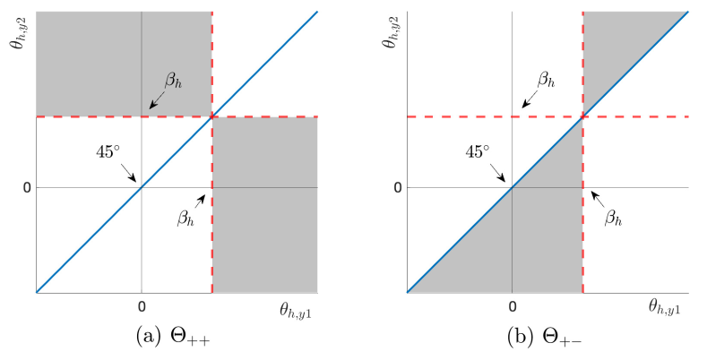
Figure 2: Identified Sets for Sign Restrictions on the Weight

One advantage of our sign restrictions strategy is that multiple instruments can be handled straightforwardly. Applying Proposition 2 to two or more instrumental variables, we construct an identified set by intersection. The shape of the identified set differs depending on the set of sign restriction imposed.

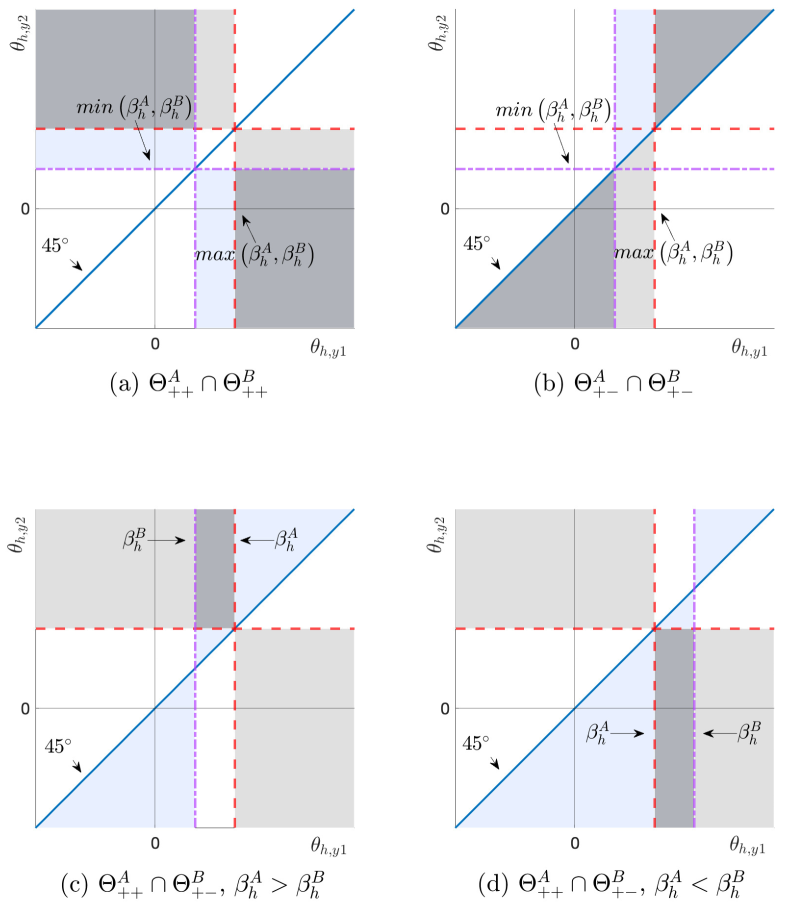
Figure 3: Intersection of Identified Sets

We illustrate the intersections in Figure 3, where the identified set by two instruments (denoted by $A$ and $B$) are shown as dark shaded areas. Let $\beta_{h}^{A}$ and $\beta_{h}^{B}$ be the IV estimand using each of the instrument $A$ and $B$ one at a time, respectively. Panel (a) shows the identified set when $w_{s}^{A}>0$ and $w_{s}^{B}>0$ for $s=1,2.$ In this case, $max(\beta_{h}^{A},\beta_{h}^{B})<\theta_{h,ys}$ if $\theta_{h,ys}>\theta_{h,ys^{\prime}}$ and $\theta_{h,ys}<min(\beta_{h}^{A},\beta_{h}^{B})$ if $\theta_{h,ys}<\theta_{h,ys^{\prime}}$ for $s,s^{\prime}=1,2$ and $s\neq s^{\prime}$. Panel (b) shows the identified set when $w_{s}^{A}>0$ and $w_{s}^{B}<0$ for $s=1,2.$ In this case, the identified set for $\theta_{h,y2}<\theta_{h,y1}<min(\beta_{h}^{A},\beta_{h}^{B})$ or $max(\beta_{h}^{A},\beta_{h}^{B})<\theta_{h,y1}<\theta_{h,y2}$. In both cases considered in Panels (a) and (b), the identified set for $\theta_{h,ys}$ depends on the value of $\theta_{h,ys^{\prime}}$ for $s,s^{\prime}=1,2$ and $s\neq s^{\prime}$.

Panels (c) and (d) show the cases where multiple instruments can provide more informative bound for the structural impulse responses. This can happen when the intersection of $\Theta_{++}^{A}$ and $\Theta_{+-}^{B}$ provides the identified set. That is, if the instrument $A$ is positively correlated with both $\varepsilon_{1,t}$ and $\varepsilon_{2,t}$ and the instrument $B$ is positively correlated with $\varepsilon_{1,t}$ but is negatively correlated with $\varepsilon_{2,t}$, then the identified set for $\theta_{h,y1}$ is $\{\theta_{h,y1}:min(\beta_{h}^{A},\beta_{h}^{B})<\theta_{h,y1}<max(\beta_{h}^{A},\beta_{h}^{B})\}$. The identified set for $\theta_{h,y2}$ depends on whether $\beta_{h}^{A}$ is larger than $\beta_{h}^{B}$ or not: If $\beta_{h}^{A}>\beta_{h}^{B}$, the set is $\{\theta_{h,y2}:\beta_{h}^{A}<\theta_{h,y2}\}$ and if $\beta_{h}^{B}>\beta_{h}^{A}$, the set is $\{\theta_{h,y2}:\beta_{h}^{A}>\theta_{h,y2}\}$. These cases correspond to the application in Section 4. We provide the detailed procedure of obtaining confidence sets for the identified set in Appendix D.2.

3.2 Identification by Granular Level Data

Suppose that we have more granular level data $x_{s,t}$ for $s=1,2$ such that $x_{t}=x_{1,t}+x_{2,t}$. For example, defense and non-defense spending data as well as the total government spending data are available. These granular data can provide point-identification of the weight $w_{s}$ under appropriate conditions. Since $w_{s}$ is point-identified, the identified set for the structural impulse responses $\theta_{h,y1}$ and $\theta_{h,y2}$ is obtained. With multiple instruments, the structural impulse responses can be point-identified.

To give a precise condition, we consider the SVMA model augmented with the granular variables (given in Appendix B). The model specifies that the granular level variables $x_{1,t}$ and $x_{2,t}$ are part of the vector moving average system so that for $s=1,2$,

$$x_{s,t}=\psi_{0,s1}\varepsilon_{1,t}+\psi_{0,s2}\varepsilon_{2,t}+\cdots+\psi_{0,sm}\varepsilon_{m,t}+\{\bm{\varepsilon}_{t-1},\bm{\varepsilon}_{t-2},\cdots\}$$

where $\psi_{0,sr}=E[x_{s,t}|\varepsilon_{r,t}=1]-E[x_{s,t}|\varepsilon_{r,t}=0]$ and $\{\cdots\}$ is a linear combination of the elements in the curly brackets. Since $x_{t}=x_{1,t}+x_{2,t}$, the baseline model (4) is a reduced SVMA model from the augmented SVMA model.

For identification of $w_{s}$, we impose that the $s$th component shock $\varepsilon_{s,t}$ does not enter the moving average representation of the granular macro variable $x_{s^{\prime},t}$ for $s\neq s^{\prime}$.

Assumption 2.

$0=\psi_{0,12}=\psi_{0,21}$ (no contemporaneous inter-sectoral causal effects)

Consider again the government spending data example. Assumption 2 is satisfied if the defense spending shock ($\varepsilon_{2,t}$) does not affect non-defense spending ($x_{1,t}$) contemporaneously and vice versa. This condition puts a similar structural restriction with the recursive causal ordering in the triangular SVAR model to identify the impulse responses. This assumption can be tested if additional instruments are available. We propose such a test in Appendix C.

Under Assumption 2, the weight $w_{s}$ is identified as

$$w_{1}=\frac{Cov(x_{1,t},z_{t})}{Cov(x_{t},z_{t})},~{}~{}w_{2}=\frac{Cov(x_{2,t},z_{t})}{Cov(x_{t},z_{t})}.$$ (16)

Now we have the following proposition.

Proposition 3.

Suppose that Assumptions 1-2 hold. The identified set for $(\theta_{h,y1},\theta_{h,y2})$ is

$$\Theta_{L}=\left\{(\theta_{h,y1},\theta_{h,y2})\left|w_{1}\theta_{h,y1}+w_{2}\theta_{h,y2}=\beta_{h}\right.\right\},$$

where $\beta_{h}$, $w_{1}$, and $w_{2}$ are functions of the observable moments.

The identified set is given by a hyperplane in $R^{2}$ (i.e., a line). Figure 4(a) illustrates the identified set $\Theta_{L}^{A}$ with the instrument $A$ when $\beta_{h}^{A}/w_{2}^{A}>0$ (intercept) and $-w_{1}^{A}/w_{2}^{A}>0$ (slope). Proposition 3 is useful in calibration analyses. For example, if the sequence of $\theta_{h,y1}$ for each $h$ is given then the corresponding sequence of $\theta_{h,y2}$ is obtained.

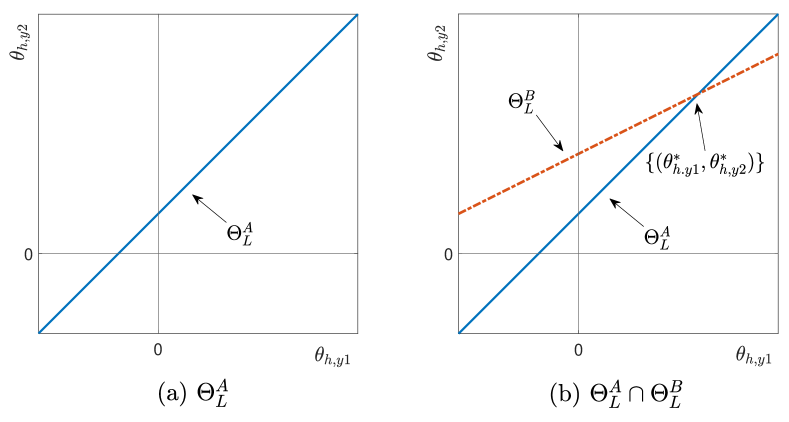
Figure 4: Identified Sets using Granular Level Data

Proposition 3 also implies that two instruments provide two distinct lines. In this case, the intersection of the identified set can be a singleton. Denote the additional instrument by superscript $B$. By using the instrument $B$, we get $\beta_{h}^{B}=Cov(y_{t+h}z_{t}^{B})/Cov(x_{t},z_{t}^{B})$, and $w_{1}^{B}$ and $w_{2}^{B}$ as in (16). Then the intersection of $\Theta_{L}^{A}$ and $\Theta_{L}^{B}$ is the solution of the simultaneous equations in matrix form:

$$\underbrace{\left(\begin{array}[]{cc}w_{1}^{A}&w_{2}^{A}\\ w_{1}^{B}&w_{2}^{B}\\ \end{array}\right)}_{\equiv W}\left(\begin{array}[]{c}\theta_{h,y1}\\ \theta_{y,h2}\end{array}\right)=\left(\begin{array}[]{c}\beta_{h}^{A}\\ \beta_{h}^{B}\end{array}\right).$$ (17)

Provided that $W$ is invertible, the solution exists and unique, which is shown as in Figure 4(b). When more than two instruments are available, the model is overidentified and a GMM type identification and estimation method can be used.

The identification strategy using more granular level data is illustrated in Section 5 to obtain the defense and non-defense spending multipliers from the LP-IV estimates of the aggregate multipliers.

4   Monetary Policy and Central Bank Information Shock

Jarociński and Karadi (2020; hereinafter JK2020) argue that central bank monetary policy shocks, such as those from the US Federal Open Market Committee (FOMC) and the European Central Bank (ECB) announcements, contain valuable information about the central bank’s assessment of economic conditions and monetary policy. JK2020 disentangles the central bank information shock from the composite monetary policy shock using Bayesian structural VAR with sign restrictions on the co-movements of the shocks in central bank announcements and high-frequency surprises in the financial markets.

In this section, we apply the sign restrictions approach described in Section 3.1 to the dataset of JK2020. Using the same sign restrictions and instruments as JK2020 but with LP-IV, we obtain set-identified impulse responses to the pure monetary policy shock, which are separated from the effect of the central bank information shock.

Let $\varepsilon_{mp,t}$ be the pure monetary policy shock, and $\varepsilon_{cb,t}$ be the central bank information shock. We assume that the FOMC announcements contain $\varepsilon_{mp,t}$ and $\varepsilon_{cb,t}$, along with other structural shocks and measurement errors, that belong to the right-hand side of the SVMA model (4). The instruments are the high-frequency surprises (the change between 10 minutes before and 20 minutes after the announcements) in the fed funds futures ($z_{t}^{ff}$) and in the stock price ($z_{t}^{sp}$). These instruments react to the central bank announcements in the very short time period, so they are assumed to be uncorrelated with any other structural shocks except for $\varepsilon_{mp,t}$ and $\varepsilon_{cb,t}$. That is, the instruments satisfy Assumption 1. The sign restrictions we impose are the same as those in Table 1 of JK2020, given by:

$$Cov(z_{t}^{ff},\varepsilon_{mp,t})>0,~{}~{}Cov(z_{t}^{ff},\varepsilon_{cb,t})>0,$$ (18)

$$Cov(z_{t}^{sp},\varepsilon_{mp,t})<0,~{}~{}Cov(z_{t}^{sp},\varepsilon_{cb,t})>0.$$ (19)

In other words, a monetary policy shock is positively correlated with the surprise in the interest rate but negatively correlated with the surprise in the stock market. On the other hand, the central bank information shock is positively correlated with the surprises in both the interest rate and the stock market.

Since the scale of $\varepsilon_{mp,t}$ and $\varepsilon_{cb,t}$ is indeterminate, the monthly average of the one-year constant-maturity Treasury yield ($x_{t}$) is used to fix the scale of the shocks. Let $z_{t}$ be either $z_{t}^{ff}$ or $z_{t}^{sp}$. According to Proposition 1, the LP-IV estimand is decomposed as follows:

$$\beta_{h}\equiv\frac{Cov(y_{t+h},z_{t})}{Cov(x_{t},z_{t})}=\frac{Cov(z_{t},\varepsilon_{mp,t})}{Cov(z_{t},x_{t})}\theta_{h,mp}+\frac{Cov(z_{t},\varepsilon_{cb,t})}{Cov(z_{t},x_{t})}\theta_{h,cb}.$$ (20)

where $Cov(z_{t},x_{t})=Cov(z_{t},\varepsilon_{mp,t})+Cov(z_{t},\varepsilon_{cb,t})$. Let’s first consider $z_{t}=z_{t}^{ff}$. Assuming that $Cov(z_{t}^{ff},x_{t})>0$ (which is justified by the data) and using the sign restrictions (18), the LP-IV estimand $\beta_{h}^{ff}$ becomes a proper weighted average of $\theta_{h,mp}$ and $\theta_{h,cb}$ since the weights are positive. Since this instrument satisfies Assumption SS, we can interpret $\beta_{h}$ as a structural impulse response to a composite monetary policy shock. In contrast, $\beta_{h}^{sp}$ using $z_{t}^{sp}$ as the instrument does not have a structural interpretation due to the opposite signs in (19).

The econometric model for LP-IV is given by:

$$y_{t+h}=\mu_{h}+\beta_{h}x_{t}+\bm{\phi}_{h}(L)^{\prime}\bm{R}_{t-1}+u_{t+h},$$ (21)

where $y_{t}$ is a macro variable of interest: the monthly average of the one-year Treasury yield, the monthly average of the S&P 500 index in log levels, the real GDP and the GDP deflator in log levels, or the excess bond premium (EBP), $\mu_{h}$ is a constant, $x_{t}$ is the monthly average of the one-year Treasury yield, and $\bm{R}_{t-1}$ is a set of control variables. These control variables include lagged values of all of the macro variables included in the impulse response analysis, as well as $x_{t}$ and the instrument $z_{t}$. $\bm{\phi}_{h}(L)$ is a coefficient vector of polynomial in the lag operator of order 12. The lag choice follows JK2020. The coefficient $\beta_{h}$ for each $h$ is the impulse response of $y_{t+h}$ to a shock that changes $x_{t}$ by one unit.

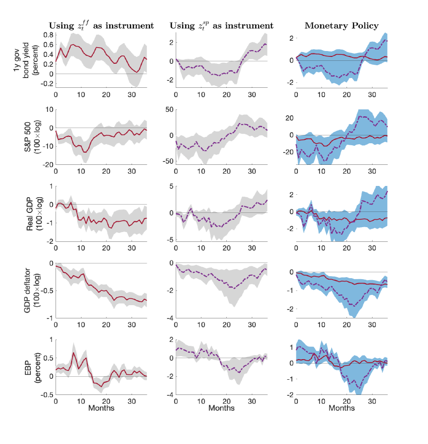
Figure 5: Identified Set for Responses to Pure Monetary Policy Shock

The first two columns in Figure 5 show $\widehat{\beta}_{h}$ in the LP-IV model (20) by using $z_{t}^{ff}$ and $z_{t}^{sp}$ one at a time, respectively. The third column shows the identified set of the impulse responses to the pure monetary policy shock obtained by imposing the sign restrictions (18)-(19) on the LP-IV estimates. The bands represent the pointwise 68% asymptotic confidence bands which are calculated using Proposition 4 in Appendix D.2. The impulse responses are with respect to 25 basis-point (BP) change in one-year government bond yield.

The impulse responses in the first column correspond to the responses to a (composite) monetary policy shock, comprising a pure monetary policy shock and a central bank information shock, identified using high-frequency surprises in the fed fund futures ($z_{t}^{ff}$). On impact, the one-year government bond yield increases by 25BP by construction, and the effect is quite persistent. Stock prices initially decline but eventually start recovering after approximately one year. The negative impact on real GDP and the price level exhibits greater persistence. The excess bond premium initially increases, but the effect is not persistent. It is important to note that the sign restrictions (18) justify the aforementioned interpretations as being legitimate and structural. Furthermore, the identified set for the structural impulse responses is given by $\Theta_{++}$ in Proposition 2, as illustrated in Figure 2(a). However, using $z_{t}^{ff}$ alone, we cannot determine the relative magnitude of the effects of pure monetary policy shocks versus central bank information shocks.

The responses identified by the high-frequency surprises in the S&P 500 index ($z_{t}^{sp}$) are presented in the second column. Combining sign restrictions (19) with $Cov(z_{t}^{sp},x_{t})<0$ (justified by the data), we argue that these responses are not a proper weighted average of the structural impulse responses. The identified set for the structural impulse responses is given by $\Theta_{+-}$ in Proposition 2, as illustrated in Figure 2(b).

By intersecting the identified sets, we obtain a more informative identified set for the impulse responses to a pure monetary policy shock. This is shown in the third column of Figure 5, which represents the areas between the two LP-IV estimates in the first two columns. The blue shaded areas indicate the identified sets with 68% pointwise confidence bands (the detailed procedure is provided in Appendix D.2). The results are highly informative. In response to a pure monetary policy shock, the interest rate response is less persistent, and the negative effects on the stock market and the price level are stronger compared to the composite monetary policy shock. This finding is also consistent with JK2020, who find “…fairly low persistence of the interest rate response and vigorous price-level decline.”

In sum, our sign restrictions approach based on LP-IV can be an attractive alternative to existing Bayesian VAR methods due to its simplicity and flexibility. For instance, if additional high-frequency instruments satisfying certain sign restrictions are available, the identified set of responses to monetary policy in Figure 5 can be further refined using additional LP-IV estimates. Furthermore, the LP-IV model (21) can be extended to include higher-order or non-linear terms, and our sign restrictions approach can still be applied.

5   Government Spending Multiplier in the U.S.

The government spending multiplier is the ratio of the change in GDP to the change in government spending. Understanding the magnitude of the multiplier is crucial for making fiscal policies, but there is still a debate in the literature about whether it is larger than one. For instance, studies by Blanchard and Perotti (2002), Barro and Redlick (2011), Ramey (2011), Auerbach and Gorodnichenko (2012), Nakamura and Steinsson (2014), and Ramey and Zubairy (2018) have explored this question extensively.

Most studies focus on estimating the aggregate or defense spending multipliers by examining variations in defense spending. This is because non-defense spending varies less than defense spending, and more importantly, non-defense spending is likely to be endogenous concerning GDP (Barro and Redlick, 2011).

In this section, we estimate the non-defense spending multiplier in the United States in the post WWII period. Building on the identification results from the previous sections, we break down the aggregate spending multipliers, which were estimated by external instruments (LP-IV estimates), into sectoral spending multipliers. To achieve this, we use granular level data and two instruments, as outlined in Figure 4(b). We focus on the post-WWII period because quarterly sectoral spending data are only available after WWII.

The LP-IV model is

$$\sum_{j=0}^{h}y_{t+j}=\mu_{h}+\beta_{h}\sum_{j=0}^{h}x_{t+j}+\bm{\phi}_{h}(L)^{\prime}\bm{R}_{t-1}+u_{t+h},$$

where $y_{t}$ is GDP, $x_{t}$ is government spending, $\bm{R}_{t}$ is a set of control variables, and $\bm{\phi}_{h}(L)$ is a coefficient vector of polynomial in the lag operator of order 4. Since $\sum_{j=0}^{h}y_{t+j}$ is the sum of GDP over $h$ periods and $\sum_{j=0}^{h}x_{t+j}$ is the sum of government spending over $h$ periods, the parameter $\beta_{h}$ is the cumulative government spending multiplier. The instrument is $z_{t}$. The control variables include lagged values of $y_{t}$, $x_{t}$, and $z_{t}$.

We use two instruments in our analysis: the military news shock from Ramey and Zubairy (2018), referred to as ‘RZ news shock’, and the current defense spending shock from Blanchard and Perotti (2002), labeled as ‘BP defense shock’. The BP defense shock is (the residual of) current defense spending. When using the ’BP defense shock’ as an IV, our control variables consist of the lagged values of GDP, government (aggregate) spending, and defense spending. This approach aligns with the construction of the Blanchard-Perotti (2002) shock in Ramey and Zubairy (2018) using current government spending.

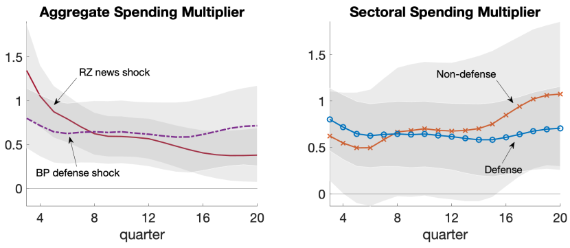
Figure 6: Cumulative Multipliers Across Different Horizons with 90% Confidence Bands. Left: aggregate spending multipliers identified by RZ news shock (solid), BP defense shock (dash-dotted). Right: non-defense spending multiplier (x), defense spending multiplier (circle)

Figure 6 presents the cumulative government spending multipliers for each horizon from two quarters to five years out. The bands are the pointwise 90% confidence bands using Newey-West (1987) standard errors. In the left panel, the cumulative government spending multipliers are depicted using the LP-IV estimates based on two different IV’s: the RZ news shock (solid line) and the BP defense shock (dash-dotted). These estimates correspond to the LHS of (9) in Corollary 1.

Consistent with Ramey and Zubairy (2018), the estimated multipliers using either of the RZ and BP shocks are below one after the first year. When the BP defense shock is used, the initial multiplier is smaller than the RZ shock but shows more prolonged effects after three years.

In the right panel of Figure 6, we present the cumulative sectoral spending multipliers derived from the two LP-IV estimates of the government spending multipliers shown in the left panel. The estimation procedure is provided in Appendix D.

The magnitude of the defense spending multiplier (circle markers) is similar to that of the aggregate spending multiplier using the BP defense shock. The cumulative non-defense spending multiplier (x markers) shows interesting trajectories, starting at around 0.7 after two years but steadily increasing past 1 after four years. This suggests a prolonged effect of non-defense spending on GDP. Additionally, the non-defense spending multiplier can exceed one, even when the government spending multipliers estimated using the RZ news shock and the BP defense shock are both below one. This is due to the negative weight assigned to the non-defense spending multiplier in the government spending multiplier decomposition.

To understand the role of weights in the government spending multiplier, we examine the decomposition of the cumulative government spending multiplier for eighteen-quarters ($h=18$). Let $s=1$ denote defense spending and $s=2$ denote non-defense spending. The government spending multiplier estimated by the RZ news shock, is then decomposed as

$$\begin{array}[]{ccccccccc}\widehat{\beta}^{RZ}_{h}&=&\widehat{w}_{h,1}^{RZ}&\times&\widehat{\frac{\widetilde{\theta}_{h,y1}}{\widetilde{\theta}_{h,x1}}}&+&\widehat{w}_{h,2}^{RZ}&\times&\widehat{\frac{\widetilde{\theta}_{h,y2}}{\widetilde{\theta}_{h,x2}}},\\ 0.37&&1.87&&0.68&&-0.87&&1.02\\ \end{array}$$ (22)

and the multiplier estimated by the BP defense shock is decomposed as

$$\begin{array}[]{ccccccccc}\widehat{\beta}^{BP}_{h}&=&\widehat{w}_{h,1}^{BP}&\times&\widehat{\frac{\widetilde{\theta}_{h,y1}}{\widetilde{\theta}_{h,x1}}}&+&\widehat{w}_{h,2}^{BP}&\times&\widehat{\frac{\widetilde{\theta}_{h,y2}}{\widetilde{\theta}_{h,x2}}}.\\ 0.69&&0.97&&0.68&&0.03&&1.02\\ \end{array}$$ (23)

Under Assumption 2, the weights are consistently estimated using sectoral spending data by

$$\widehat{w}_{h,s}^{(j)}=\frac{\sum_{t=1}^{T-h}z_{t}^{\perp(j)}\left(\sum_{j=0}^{h}x_{s,t+j}^{\perp(j)}\right)}{\sum_{t=1}^{T-h}z_{t}^{\perp(j)}\left(\sum_{j=0}^{h}x_{t+j}^{\perp(j)}\right)},$$

where $j$ denotes the RZ news shock or the BP defense shock and $v_{t}^{\perp(j)}$ denotes the residual of $v_{t}$ after regressing it on the set of control variables including the lagged values of the instrument $j$. The estimated weights show similar magnitudes and signs across different $h$ for both instruments.

The decomposition (22)-(23) reveals that the government spending multiplier estimated using the RZ news shock is smaller than both sectoral spending multipliers due to the negative weight assigned to the non-defense spending multiplier in (22). This indicates a violation of the same-sign condition (Assumption SS) for the RZ news shock as an IV. The positive military news shock leads to a positive impact on defense spending, but at the same time, it has a negative impact on non-defense spending. Consequently, the positive non-defense spending multiplier has a negative effect on GDP, thereby underestimating the sectoral spending multipliers. This raises concerns about the structural interpretation of the government spending multiplier estimated using the RZ news shock.

In contrast, for the government spending multiplier estimated using the BP defense shock, both weights have positive signs, but the weight for the non-defense spending multiplier is very small (0.03). As a result, the government spending multiplier estimated by the BP defense shock closely resembles the defense spending multiplier.

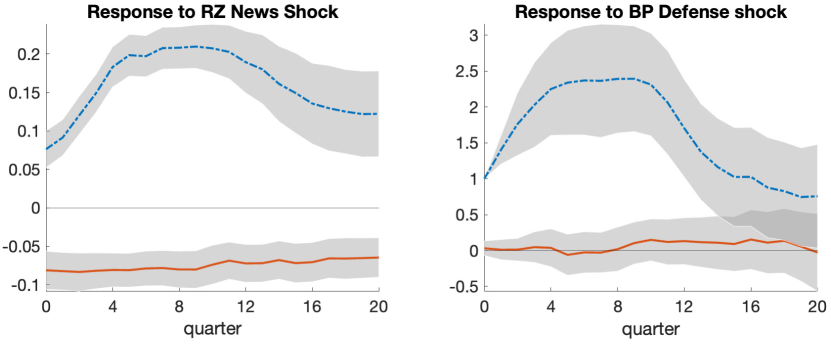
Figure 7: Impulse Response of Sectoral Spending to the Instruments with 90% Confidence Bands: Defense spending (dash-dotted), Non-defense spending (solid)

Figure 7 shows the impulse response of defense spending (dash-dotted line) and non-defense spending (solid line) to the RZ news shock (left panel) and to the BP defense shock (right panel). Note that the dependent variables are sectoral spending ($x_{s,t+h}$), rather than the cumulative sectoral spending ($\sum_{j=0}^{h}x_{s,t+j}$).

The RZ news shock has a relatively small but statistically significant negative effect on non-defense spending. In contrast, the response of non-defense spending to the BP defense shock is statistically insignificant for all $h$. Given that the decomposition (23) suggests that the BP defense shock closely approximates the structural defense spending shock, the insignificant response of non-defense spending to the BP shock supports the cumulative version of Assumption 2.

5.1 Further Analysis

In this subsection, we address two cases: (I) when the weights cannot be point-identified due to the lack of granular level data but sign restrictions can be imposed, and (II) when granular level data are available, but the number of instruments is smaller than the number of components.

First consider Case (I), which can be analyzed using the identification method described in Section 3.1. In this scenario, we cannot point-identify the weights because sectoral level spending data are unavailable. We use GDP, total government spending, and the two instruments. We impose the following restrictions:

1. $\widetilde{\theta}_{h,xs}\geq 0$ for $h=1,2,...,H$ and $s=1,2$: Both of defense and non-defense spending shocks have positive effects on the cumulative government spending over the $h$ periods.

2. $Cov(z_{t}^{RZ},\varepsilon_{1,t})>0$: The RZ news shock is positively correlated with a defense spending shock.

3. $Cov(z_{t}^{RZ},\varepsilon_{2,t})<0$: The RZ news shock is negatively correlated with a non-defense spending shock.

4. $Cov(z_{t}^{BP},\varepsilon_{2,t})=0$: The BP defense shock is uncorrelated with a non-defense spending shock.

The restrictions (i) and (ii) are straightforward. (iii) is based on the government budget constraint argument. (iv) is a structural restriction similar to the ordering of endogenous variables in the SVAR model.

According to Corollary 1,

$$\beta_{h}^{j}=\frac{Cov(z_{t}^{j},\varepsilon_{1,t})\widetilde{\theta}_{h,x1}}{Cov(z_{t}^{j},\widetilde{x}_{t+h})}\times\frac{\widetilde{\theta}_{h,y1}}{\widetilde{\theta}_{h,x1}}+\frac{Cov(z_{t}^{j},\varepsilon_{2,t})\widetilde{\theta}_{h,x2}}{Cov(z_{t}^{j},\widetilde{x}_{t+h})}\times\frac{\widetilde{\theta}_{h,y2}}{\widetilde{\theta}_{h,x2}},$$ (24)

for $j=RZ,BP$. The restriction (iv) implies that $\beta_{h}^{BP}=\widetilde{\theta}_{h,y1}/\widetilde{\theta}_{h,x1}$. That is, the cumulative defense spending multiplier is point-identified by the LP-IV estimand using the BP defense shock. The restrictions (i)-(iii) determine the sign of the weight in the decomposition using the RZ news shock as the instrument because the sample estimates of $Cov(z_{t}^{RZ},\widetilde{x}_{t+h})$ are positive for $h\geq 1$. This set corresponds to $\Theta_{+-}$ in Proposition 2. By intersecting the identified sets, we can obtain the identified set for the cumulative sectoral spending multipliers.

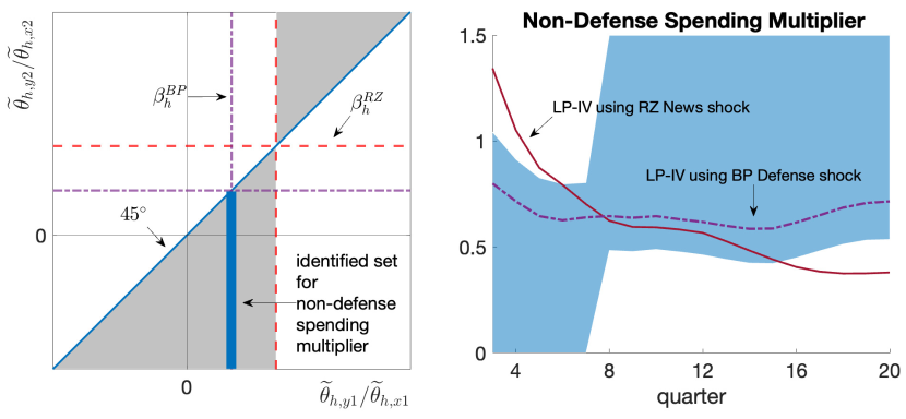
Figure 8: Identified Set for Non-Defense Spending Multiplier using Sign Restrictions and Two IVs. Left panel: $\widetilde{\theta}_{h,y1}/\widetilde{\theta}_{h,x1}$ is the defense spending multiplier and $\widetilde{\theta}_{h,y2}/\widetilde{\theta}_{h,x2}$ is the non-defense spending multiplier. Right panel: The blue shaded area is the set-identified non-defense spending multiplier with 68% confidence bands.

Figure 8 displays the intersection of the identified set (left panel) and the set-identified non-defense spending multiplier with 68% confidence bands (right panel).

In the left panel, the shaded areas represent the identified set based on the sign restrictions (i)-(iii). Since the LP-IV estimand using the BP defense shock as the instrument is equivalent to the defense spending multiplier due to (iv), the intersection is represented by a line assuming $\beta_{h}^{BP}<\beta_{h}^{RZ}$. In this scenario, $\beta_{h}^{BP}$ serves as the upper bound for the non-defense spending multiplier. Conversely, if $\beta_{h}^{BP}>\beta_{h}^{RZ}$, $\beta_{h}^{BP}$ becomes the lower bound. Additionally, we calculate the pointwise (for each $h$) confidence interval for the identified set using the formula provided in Appendix D.2. The resulting set is shown on the right panel.

The non-defense spending multiplier is bounded above by the LP-IV estimate using the BP defense shock until approximately two years, and from then onwards, it is bounded below. It is noteworthy that the point estimates of the non-defense spending multipliers in Figure 6 fall within the identified set presented in Figure 8. This demonstrates that our sign restrictions approach can provide an informative bounds for the componentwise impulse responses even in situations where granular level data is unavailable.

In Case (II), when only granular level data and one instrument are available, we use GDP, total government spending, defense and non-defense spending, and the RZ news shock instrument. The LP-IV estimand using the RZ news shock instrument can be decomposed according to (24). Under Assumptions 1 and 2, the weights are identified as

$$w_{h,1}=\frac{E[z_{t}\widetilde{x}_{1,t+h}]}{E[z_{t}\widetilde{x}_{t+h}]},~{}~{}w_{h,2}=\frac{E[z_{t}\widetilde{x}_{2,t+h}]}{E[z_{t}\widetilde{x}_{t+h}]},$$

where $\widetilde{x}_{1,t}$ and $\widetilde{x}_{2,t}$ are cumulative defense and non-defense spending, respectively. By Proposition 3, we obtain the identified set $\Theta_{L}$ for $(\widetilde{\theta}_{h,y1}/\widetilde{\theta}_{h,x1},\widetilde{\theta}_{h,y2}/\widetilde{\theta}_{h,x2})$.

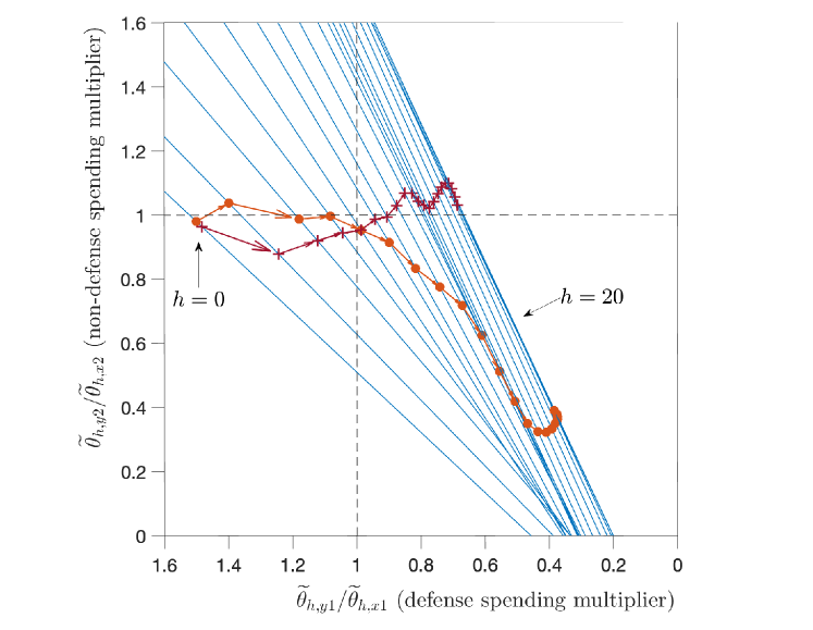
Figure 9: Identified Set for Sectoral Spending Multipliers using Sectoral Spending Data and the RZ News Shock Instrument. $\bullet$: Calibrated defense spending multiplier is transitory; $+$: Calibrated defense spending multiplier is persistent.

Figure 9 illustrates the identified set $\Theta_{L}$ for each $h=0,...,20$ (represented by blue solid lines). As $h$ increases, the lines exhibit steeper slopes with larger y-intercepts. This observation implies that as time progresses, for a given magnitude of the defense spending multiplier (x-axis), the corresponding magnitude of the non-defense spending multiplier becomes larger.

More specifically, to achieve a non-defense spending multiplier greater than one, the magnitude of the defense spending multiplier needs to be larger than 1.5 when $h=0$ (immediate impact), but only 0.67 when $h=20$ (five years out).

The identified set can also be used for counterfactual analyses using calibration. For this purpose, we calibrate the defense spending multiplier based on the result of Auerbach and Gorodnichenko (2012) and Barro and Redlick (2011). We consider two trajectories of the defense spending multiplier: transitory and persistent. Both calibrations set the defense spending multiplier is 1.5 on impact, but the transitory defense spending multiplier declines more rapidly than the persistent defense spending multiplier, reaching 0.67 after two years, rather than 0.85 which is the persistent multiplier case.

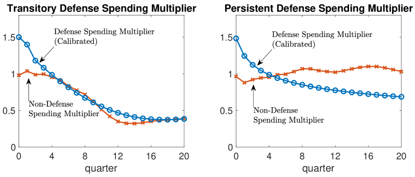
Figure 10: Sectoral Spending Multipliers using Calibration

In Figure 9, we observe two trajectories of the sectoral spending multipliers represented by circle and plus markers. Each trajectory corresponds to a specific calibrated defense spending multiplier value from the identified set for each $h$, as shown in Figure 10.

The results highlight that even a small difference in the magnitude of the defense spending multiplier can lead to a substantial difference in the non-defense spending multiplier. Particularly, if the magnitude of the defense spending multiplier remains around 0.8 persistently after two years, then the non-defense spending multiplier can exceed one, even when the aggregate and defense spending multipliers are below one.

6   Conclusion

This paper presents the first formal analysis of the identification power of the LP-IV approach in a more empirically relevant setting, along with a systematic method for incorporating sign restrictions within the LP-IV framework.

On one hand, our findings caution that the robustness of the IV approach depends on the specific situation, and problematic cases can arise in practical applications. On the other hand, we demonstrate that the problematic LP-IV estimand can be transformed into valuable information when multiple IVs are available, as it facilitates the generation of informative identified intervals for structural parameters.

Given the simplicity, flexibility, and widespread use of the LP-IV approach in empirical studies, our discovery that it can effectively handle multiple IVs and sign restrictions will enable researchers to apply it in a more diverse range of cases and interpret outcomes more reasonably. This is likely to foster greater adoption of the LP-IV approach in various research contexts.

Appendix

Appendix A Proofs

A.1 Proof of Proposition 1

Write $y_{t+h}$ and $x_{t+h}$ as

$$y_{t+h}= \sum_{j=0}^{\infty}\left(\sum_{s=1}^{S}\theta_{j,ys}\varepsilon_{s,t+h-j}+\sum_{r=S+1}^{m}\theta_{j,yr}\varepsilon_{r,t+h-j}\right),$$

$$x_{t+h}= \sum_{j=0}^{\infty}\left(\sum_{s=1}^{S}\theta_{j,xs}\varepsilon_{s,t+h-j}+\sum_{r=S+1}^{m}\theta_{j,xr}\varepsilon_{r,t+h-j}\right).$$

By Assumption 1 and the unit effect normalization, we obtain

$$Cov(y_{t+h},z_{t})= E[y_{t+h}z_{t}]=\sum_{s=1}^{S}E[z_{t}\varepsilon_{s,t}]\theta_{h,ys}=\sum_{s=1}^{S}\alpha_{s}\theta_{h,ys},$$

$$Cov(x_{t},z_{t})= E[x_{t}z_{t}]=\sum_{s=1}^{S}E[z_{t}\varepsilon_{s,t}]\theta_{0,xs}=\sum_{s=1}^{S}\alpha_{s},$$

as desired. ∎

A.2 Proof of Corollary 1

The proof is similar to the proof of Proposition 1, and thus omitted.

Appendix B Augmented SVMA

The augmented SVMA model extends the baseline SVMA model (4) to include the granular level variables, $x_{s,t}$ for $s=1,2,...,S$ such that $x_{t}=\sum_{s=1}^{S}x_{s,t}$. The $x_{s,t}$’s are the components of the aggregate variable $x_{t}$. To avoid unnecessary confusion, we call $s$ as sectors and $x_{s,t}$ as sectoral variables, although they do not necessarily have to be. The augmented SVMA model is given by

$$\bm{Y}_{t}^{A}=\bm{\Psi}(L)\bm{\varepsilon}_{t}$$ (25)

where $\bm{Y}_{t}^{A}=(x_{1,t},x_{2,t},...,x_{S,t},...,y_{t})^{\prime}$ is an $(n+S-1)\times 1$ vector of observed endogenous variables, $\bm{\Psi}(L)=\bm{\Psi}_{0}+\bm{\Psi}_{1}L+\bm{\Psi}_{2}L^{2}+\cdots$, and $\bm{\Psi}_{h}$ for $h=0,1,2,...,$ is an $(n+S-1)\times m$ matrix of impulse responses. Let $\bm{B}=(\bm{i}_{n}~{}\bm{i}_{n}~{}\cdots~{}\bm{i}_{n}~{}\bm{I}_{n})$ be the $n\times(n+S-1)$ matrix where $\bm{i}_{n}=(1,0,...,0)^{\prime}$ and $\bm{I}_{n}$ is the $n\times n$ identity matrix. By pre-multiplying $\bm{B}$ both sides of (25), we can obtain (4) and $\bm{\Theta}(L)=\bm{B}\bm{\Psi}(L)$. Without any further restrictions on the impulse response matrices, (25) is more general than (4). Note that the last $n-1$ rows of $\bm{\Psi}(L)$ are identical to the last $n-1$ rows of $\bm{\Theta}(L)$.

Let $\psi_{h,rs}$ be the response of sectoral variable $x_{r,t+h}$ to the shock $\varepsilon_{s,t}$. This impulse response is the $(r,s)$-th element of $\bm{\Psi}_{h}$. With the unit effect normalization for each sectoral shock ($\psi_{0,ss}=1$ for $s=1,2,...,S$), $\varepsilon_{s,t}$ is scaled so that one unit change in $\varepsilon_{s,t}$ corresponds to the unit change in $x_{s,t}$. For example, if $x_{1,t}$ and $x_{2,t}$ are non-defense and defense spending and $\varepsilon_{1,t}$ and $\varepsilon_{2,t}$ are the corresponding sectoral spending shocks, then a positive unit sectoral spending shock increases the corresponding sectoral spending by one unit.

For the componentwise impulse responses in the augmented SVMA model to be identified we need a restriction on $\bm{\Psi}_{0}$ that there is no contemporaneous inter-sectoral causal effects, i.e., for all $r,s=1,2,...,S$ and $r\neq s$,

$$0=E[x_{r,t}|\varepsilon_{s,t}=1]-E[x_{r,t}|\varepsilon_{s,t}=0].$$ (26)

In other words, the $s$-th sectoral shock $\varepsilon_{s,t}$ does not enter the moving average representation of the $r$-th sectoral observation $x_{r,t}$ where $r\neq s$. The condition is formally stated as follows:

Assumption 2^′.

For all $r\neq s$ and $r,s\in\mathcal{S}_{\xi}$, $\psi_{0,rs}=0$.

Assumption 2^′ may be tested if we have enough number of instruments. A formal testing procedure is given in Appendix Section C. Note that $\psi_{0,ss}=\theta_{0,xs}=1$ under Assumption 2^′ and the unit effect normalization.

Appendix C Testing No Inter-Sectoral Causal Effects

Assumption 2^′ can be tested by the generalized method of moments (GMM). The idea is to jointly estimate the componentwise impulse responses $\psi_{0,rs}$ and $\theta_{h,ys}$ for $r,s=1,2,...,S$ by GMM and then test $\psi_{0,rs}=0$ for $r\neq s$.

Let $\bm{Z}_{t}$ be an $l\times 1$ vector of instruments and $\bm{X}_{t}=(x_{1,t},x_{2,t},\cdots,x_{S,t})^{\prime}$ be the $S\times 1$ vector of sectoral observations. We require that the instruments are jointly relevant, which is Assumption 3^′.

Assumption 3^′.

$rank(E[\bm{Z}_{t}\bm{X}_{t}^{\prime}])=S$.

A necessary condition for Assumption 3^′ is $l\geq S$.

Let $\bm{e}_{t}\equiv(\varepsilon_{1,t},\varepsilon_{2,t},...,\varepsilon_{S,t})^{\prime}$, $\bm{\Lambda}\equiv E[\bm{Z}_{t}\bm{e}_{t}^{\prime}]$, and $\bm{\theta}_{h,y}\equiv(\theta_{h,y1},...,\theta_{h,yS})^{\prime}$. Also let $\bm{\Psi}_{0,X}$ be the $S\times S$ upper left submatrix of $\bm{\Psi}_{0}$ in the augmented SVMA model (25). Assuming the unit effect normalization, but not assuming Assumption 2^′, $\bm{\Psi}_{0,X}$ is given by

$$\bm{\Psi}_{0,X}=\left(\begin{array}[]{cccc}1&\psi_{0,12}&\cdots&\psi_{0,1S}\\ \psi_{0,21}&1&\cdots&\psi_{0,2S}\\ \vdots&\vdots&\vdots&\vdots\\ \psi_{0,S1}&\psi_{0,S2}&\cdots&1\end{array}\right).$$

Since $E[\bm{Z}_{t}x_{s,t}]=\bm{\Lambda}\times(\psi_{0,s1},\psi_{0,s2},...,\psi_{0,sS})^{\prime}$,

$$Cov(\bm{Z}_{t},\bm{X}_{t}^{\prime})=E[\bm{Z}_{t}\bm{X}_{t}^{\prime}]=\bm{\Lambda}\bm{\Psi}_{0,X}^{\prime}.$$ (27)

Assume that $\bm{\Psi}_{0,X}$ is invertible. Plugging $E[\bm{Z}_{t}\bm{X}_{t}^{\prime}]\bm{\Psi}_{0,X}^{-1^{\prime}}=\bm{\Lambda}$ from (27) into $E[\bm{Z}_{t}y_{t+h}]=\bm{\Lambda}\bm{\theta}_{h,y}$, we have the moment condition

$$E[\bm{Z}_{t}(y_{t+h}-\bm{X}_{t}^{\prime}\bm{\Psi}_{0,X}^{-1^{\prime}}\bm{\theta}_{h,y})]=0.$$

Since the number of unknown parameters is $S^{2}$, i.e., $S^{2}-S$ unknown elements in $\bm{\Psi}_{0,X}$ plus $S$ unknown elements in $\bm{\theta}_{h,y}$, if at least $l=S^{2}$ instruments are available then a necessary condition for identification is satisfied. Since the moment condition is nonlinear in the parameters, having as many instruments as the unknown parameters does not necessarily imply global identification. In general, finding primitive conditions for identification of parameters in a nonlinear model is difficult (Newey and McFadden, 1994, p.2127). Nevertheless, by assuming identification, Assumption 2^′ can be written as the null hypothesis:

$$H_{0}:~{}\bm{\Psi}_{0,X}=I_{S}$$

where $I_{S}$ is the $S\times S$ identity matrix. We can use the GMM based tests such as the Wald test or the Lagrange multiplier test.

Appendix D Estimation and Inference

In this section, we provide estimation and inference procedures for the empirical results in the main text.

D.1 LP-IV Estimator and Standard Error

The LP-IV model is a single equation linear IV model given by

$$y_{t+h}=x_{t}\beta_{h}+\bm{R}_{t}^{\prime}\bm{\gamma}_{h}+u_{t+h},$$ (28)

for $t=1,2,...,T$ and $h=0,1,2,...,H$, where the control variables $\bm{R}_{t}$ include a constant and the lagged values of the endogenous variable and the instrument.

The parameters $(\beta_{h},\bm{\gamma}_{h}^{\prime})$ are estimated by the IV regression using $(z_{t},\bm{R}_{t}^{\prime})$ as the IV for $(x_{t},\bm{R}_{t}^{\prime})$. The LP-IV estimator is

$$\left(\begin{array}[]{c}\widehat{\beta}_{h}\\ \widehat{\bm{\gamma}}_{h}\end{array}\right)=\left(\sum_{t=1}^{T-h}\left[\begin{array}[]{cc}z_{t}x_{t}&z_{t}\bm{R}_{t}^{\prime}\\ \bm{R}_{t}x_{t}&\bm{R}_{t}\bm{R}_{t}^{\prime}\\ \end{array}\right]\right)^{-1}\sum_{t=1}^{T-h}\left(\begin{array}[]{c}z_{t}y_{t+h}\\ \bm{R}_{t}y_{t+h}\end{array}\right).$$

We use the Newey-West standard errors based on the heteroskedasticity and autocorrelation robust covariance matrix estimator.

D.2 Confidence Intervals for the Identified Set

We present how to construct a confidence interval for the identified set. We focus on the case of two IVs, which covers the applications in the main text.

Let $\widehat{\bm{\beta}}$ be the bivariate IV estimates for a given $h$. Suppose that $\sqrt{T}\left(\widehat{\bm{\beta}}-\bm{\beta}\right)\xrightarrow{d}N\left(0,\Sigma\right)$ and $\widehat{\Sigma}$ is a consistent estimator of the asymptotic variance $\Sigma$. The sample size is $T$. For a bivariate random vector $X\sim N\left(0,\Sigma\right)$, let

$$p\left(c_{1},c_{2},\Sigma\right)=\Pr\left\{X_{1}\leq c_{1},X_{2}>-c_{2}\right\}$$

where $X_{1}$ and $X_{2}$ are the first and second elements of $X$, respectively. Define

$$\left(c_{10},c_{20}\right)=\arg\min_{c_{1},c_{2}\geq 0}\left(c_{1}+c_{2}\right)\quad\text{s.t. }\quad p\left(c_{1,}c_{2},\Sigma\right)=1-\alpha,$$ (29)

for a given $\alpha>0$ and $\Sigma$. Also, let $\left(\widehat{c}_{1},\widehat{c}_{2}\right)$ denote the solution of (29) when $\Sigma=\widehat{\Sigma}$.

Let $\beta_{1}$ and $\beta_{2}$ be the first and the second elements of $\bm{\beta}$ and let $\theta$ be the componentwise impulse response. Depending on the imposed sign restrictions, we will be in one of the following situations: $\left(i\right)$ $\beta_{1}\leq\theta\leq\beta_{2}$, $\left(ii\right)$ $\beta_{2}\leq\theta\leq\beta_{1}$, $\left(iii\right)$ $\beta_{1},\beta_{2}\leq\theta$, and $\left(iv\right)$ $\beta_{1},\beta_{2}\geq\theta$. For each case, we propose the confidence interval as follows:

• $\left(i\right)$$\beta_{1}\leq\theta\leq\beta_{2}$ or $\left(ii\right)$ $\beta_{2}\leq\theta\leq\beta_{1}$. Introduce

  $$\mathcal{C}_{1n}=\left[\widehat{\beta}_{1}-\frac{\widehat{c}_{1}}{\sqrt{T}},\widehat{\beta}_{2}+\frac{\widehat{c}_{2}}{\sqrt{T}}\right].$$

  if $\widehat{\beta}_{1}<\widehat{\beta}_{2}$, and

  $$\mathcal{C}_{2n}=\left[\widehat{\beta}_{2}-\frac{\widehat{c}_{2}}{\sqrt{T}},\widehat{\beta}_{1}+\frac{\widehat{c}_{1}}{\sqrt{T}}\right],$$

  otherwise. Then, the confidence set for $\theta$ is written as

  $$\mathcal{C}_{n}=\left(\mathcal{C}_{1n}\cap\left\{\widehat{\beta}_{1}<\widehat{\beta}_{2}\right\}\right)\cup\left(\mathcal{C}_{2n}\cap\left\{\widehat{\beta}_{1}>\widehat{\beta}_{2}\right\}\right).$$

• $\left(iii\right)$ $\beta_{1},\beta_{2}\leq\theta$. Then, the confidence interval for $\theta$ is given by

  $$\mathcal{C}_{3n}=\left[\widehat{\beta}_{\widehat{i}}-\frac{\widehat{q}_{1-\alpha}}{\sqrt{T}},\infty\right),$$

  where $\widehat{q}_{1-\alpha}$ denotes the $\left(1-\alpha\right)$ quantile of $\max_{i=1,2}\left\{X_{i}\right\}$ when $\Sigma=\widehat{\Sigma}$ and $\widehat{i}$ be the index of $\arg_{i=1,2}\max\left\{\widehat{\beta}_{i}\right\}$.

• $\left(iv\right)$ $\beta_{1},\beta_{2}\geq\theta$. Then, the confidence interval for $\theta$ is given by

  $$\mathcal{C}_{4n}=\left(-\infty,\widehat{\beta}_{\widehat{i}}+\frac{\widehat{q}_{1-\alpha}}{\sqrt{T}}\right],$$

  Note that since $X$ is a centered bivariate normal, it implies $\max_{i=1,2}\{X_{i}\}\stackrel{{\scriptstyle d}}{{=}}\max_{i=1,2}\{-X_{i}\}$ and thus $\min_{i=1,2}\{X_{i}\}\stackrel{{\scriptstyle d}}{{=}}-\max_{i=1,2}\{X_{i}\}$.

Proposition 4.

The coverage probability of $\mathcal{C}_{n}$, $\mathcal{C}_{3n}$, or $\mathcal{C}_{4n}$ converges to $1-\alpha$ under each scenario.

Proof.

First note that $\widehat{c}_{1}$ and $\widehat{c}_{2}$ are positive and converges in probability to $c_{1}$ and $c_{2}$, respectively, due to the consistency of $\widehat{\Sigma}$. We give the proof of the first two cases.

First consider Case (i) with $\beta_{1}\leq\theta\leq\beta_{2}$. If $\beta_{1}<\beta_{2}$, $\widehat{\beta}_{1}<\widehat{\beta}_{2}$ with probability approaching one and

$$\Pr\left\{\theta\in\mathcal{C}_{1n}\right\}\geq\Pr\left\{\widehat{\beta}_{1}-\frac{\widehat{c}_{1}}{\sqrt{n}}\leq\beta_{1}\text{ and }\beta_{2}\leq\widehat{\beta}_{2}+\frac{\widehat{c}_{2}}{\sqrt{n}}\right\}\to 1-\alpha,$$

where the inequality holds because $\left\{\left(a,b\right):a\leq\beta_{1}\text{ and }\beta_{2}\leq b\right\}\subset\left\{\left(a,b\right):a\leq\theta\leq b\right\}$ due to the fact $\beta_{1}\leq\theta\leq\beta_{2}$. The same reasoning applies for the case of $\beta_{1}>\beta_{2}$. Thus, we obtain the correct coverage.

Next, suppose that $\beta_{1}=\beta_{2}=\theta$. Then, $\theta\in\mathcal{C}_{1n}\cap\left\{\widehat{\beta}_{1}<\widehat{\beta}_{2}\right\}$ implies the following event

$$\left\{\sqrt{n}\left(\widehat{\beta}_{1}-\beta_{1}\right)\leq\widehat{c}_{1},-\widehat{c}_{2}\leq\sqrt{n}\left(\widehat{\beta}_{2}-\beta_{2}\right)\text{ and }\widehat{\beta}_{1}<\widehat{\beta}_{2}\right\}.$$

Similarly, $\theta\in\mathcal{C}_{2n}\cap\left\{\widehat{\beta}_{1}>\widehat{\beta}_{2}\right\}$ implies the following event

$$\left\{\sqrt{n}\left(\widehat{\beta}_{1}-\beta_{1}\right)\geq-\widehat{c}_{2},\widehat{c}_{1}\geq\sqrt{n}\left(\widehat{\beta}_{2}-\beta_{2}\right)\text{ and }\widehat{\beta}_{1}>\widehat{\beta}_{2}\right\}.$$

The union of the two contains the set $\left\{\sqrt{n}\left(\widehat{\beta}_{1}-\beta_{1}\right)\geq-\widehat{c}_{2},\widehat{c}_{1}\geq\sqrt{n}\left(\widehat{\beta}_{2}-\beta_{2}\right)\right\}$, whose probability converges to $1-\alpha$ due to the definition of the convergence in distribution and the construction of $\widehat{c}_{i}$, $i=1,2$. Then, $\lim_{n}\Pr\left\{\theta\in\mathcal{C}_{1n}\right\}\geq 1-\alpha$.

Now consider Case $\left(iii\right)$ $\beta_{1},\beta_{2}\leq\theta$. The coverage probability of $\mathcal{C}_{3n}$ is easily justified if $\beta_{1}\neq\beta_{2}$ since in that case one estimator is greater than the other with probability approaching 1. Note that $q_{1-\alpha}$ is greater than the $\left(1-\alpha\right)$ quantile of an element in $X$. If $\beta_{1}=\beta_{2}=\beta$, then

$$\sqrt{n}\left(\max_{i}\left\{\widehat{\beta}_{i}\right\}-\beta\right)=\max_{i}\left\{\sqrt{n}\left(\widehat{\beta}_{i}-\beta\right)\right\}\to^{d}\max_{i}\left\{X_{i}\right\},$$

due to the continuous mapping theorem as required. The proof for Case $\left(iv\right)$ $\beta_{1},\beta_{2}\geq\theta$ is analogous and omitted. ∎

References

- [1] Adao, R., Kolesár, M., & Morales, E. (2019). Shift-share designs: Theory and inference. The Quarterly Journal of Economics, 134(4), 1949-2010.
- [2] Angrist, J. D., Imbens, G. W., & Rubin, D. B. (1996). Identification of causal effects using instrumental variables. Journal of the American Statistical Association, 91(434), 444-455.
- [3] Angrist, J. D., & Kuersteiner, G. M. (2011). Causal effects of monetary shocks: Semiparametric conditional independence tests with a multinomial propensity score. Review of Economics and Statistics, 93(3), 725-747.
- [4] Auerbach, A. J., & Gorodnichenko, Y. (2012). Measuring the output responses to fiscal policy. American Economic Journal: Economic Policy, 4(2), 1-27.
- [5] Barro, R. J., & Redlick, C. J. (2011). Macroeconomic effects from government purchases and taxes. The Quarterly Journal of Economics, 126(1), 51-102.
- [6] Blanchard, O., & Perotti, R. (2002). An empirical characterization of the dynamic effects of changes in government spending and taxes on output. The Quarterly Journal of Economics, 117(4), 1329-1368.
- [7] Borusyak, K., Hull, P., & Jaravel, X. (2022). Quasi-experimental shift-share research designs. The Review of Economic Studies, 89(1), 181-213.
- [8] Bouakez, H., Rachedi, O., & Santoro, E. (2020). The sectoral origins of the spending multiplier. Working paper.
- [9] Cox, L., Müller, G., Pasten, E., Schoenle, R., & Weber, M. (2020). Big G (No. w27034). National Bureau of Economic Research.
- [10] de Chaisemartin, C., & d’Haultfoeuille, X. (2020). Two-way fixed effects estimators with heterogeneous treatment effects. American Economic Review, 110(9), 2964-2996.
- [11] Gertler, M., & Karadi, P. (2015). Monetary policy surprises, credit costs, and economic activity. American Economic Journal: Macroeconomics, 7(1), 44-76.
- [12] Granziera, E., Moon, H. R., & Schorfheide, F. (2018). Inference for VARs identified with sign restrictions. Quantitative Economics, 9(3), 1087-1121.
- [13] Goldsmith-Pinkham, P., Sorkin, I., & Swift, H. (2020). Bartik instruments: What, when, why, and how. American Economic Review, 110(8), 2586-2624.
- [14] Imbens, G. W., & Angrist, J. D. (1994). Identification and Estimation of Local Average Treatment Effects. Econometrica, 62(2), 467-475.
- [15] Jarociński, M., & Karadi, P. (2020). Deconstructing monetary policy surprises—the role of information shocks. American Economic Journal: Macroeconomics, 12(2), 1-43.
- [16] Jordà, Ò. (2005). Estimation and inference of impulse responses by local projections. American Economic Review, 95(1), 161-182.
- [17] Jordà, Ò., Schularick, M., & Taylor, A. M. (2015). Betting the house. Journal of International Economics, 96, S2-S18.
- [18] Jordà, Ò., Schularick, M., & Taylor, A. M. (2020). The effects of quasi-random monetary experiments. Journal of Monetary Economics, 112, 22-40.
- [19] Kaminska, I., Mumtaz, H., & S̆ustek, R. (2021). Monetary policy surprises and their transmission through term premia and expected interest rates. Journal of Monetary Economics, 124, 48-65.
- [20] Mertens, K., & Ravn, M. O. (2013). The dynamic effects of personal and corporate income tax changes in the United States. American Economic Review, 103(4), 1212-47.
- [21] Mogstad, M., Torgovitsky, A., & Walters, C. R. (2021). The causal interpretation of two-stage least squares with multiple instrumental variables. American Economic Review, 111(11), 3663-3698.
- [22] Montiel Olea, J. L., & Pflueger, C. (2013). A robust test for weak instruments. Journal of Business & Economic Statistics, 31(3), 358-369.
- [23] Montiel Olea, J. L., & Plagborg-Møller, M. (2021). Local projection inference is simpler and more robust than you think. Econometrica, 89(4), 1789-1823.
- [24] Moon, H. R., & Schorfheide, F. (2012). Bayesian and frequentist inference in partially identified models. Econometrica, 80(2), 755-782.
- [25] Nakamura, E., & Steinsson, J. (2014). Fiscal stimulus in a monetary union: Evidence from US regions. American Economic Review, 104(3), 753-92.
- [26] Nakamura, E., & Steinsson, J. (2018). Identification in macroeconomics. Journal of Economic Perspectives, 32(3), 59-86.
- [27] Newey, W. K., & McFadden, D. (1994). Large sample estimation and hypothesis testing. Handbook of econometrics, 4, 2111-2245.
- [28] Newey, W. K., & West, K. D. (1987). A simple, positive semi-definite, heteroskedasticity and autocorrelation consistent covariance matrix. Econometrica, 55(3), 703-708.
- [29] Plagborg-Møller, M., & Wolf, C. K. (2021). Local projections and VARs estimate the same impulse responses. Econometrica, 89(2), 955-980.
- [30] Plagborg-Møller, M., & Wolf, C. K. (2022). Instrumental variable identification of dynamic variance decompositions. Journal of Political Economy, 130(8), 2164-2202.
- [31] Ramey, V. A. (2011). Identifying government spending shocks: It’s all in the timing. The Quarterly Journal of Economics, 126(1), 1-50.
- [32] Rambachan, A., & Shepherd, N. (2021). When do common time series estimands have nonparametric causal meaning?. Working paper.
- [33] Ramey, V. A., & Zubairy, S. (2018). Government spending multipliers in good times and in bad: evidence from US historical data. Journal of Political Economy, 126(2), 850-901.
- [34] Stock, J. H., & Watson, M. W. (2012). Disentangling the Channels of the 2007-2009 Recession (No. w18094). National Bureau of Economic Research.
- [35] Stock, J. H., & Watson, M. W. (2018). Identification and estimation of dynamic causal effects in macroeconomics using external instruments. The Economic Journal, 128(610), 917-948.
- [36] Uhlig, H. (2005). What are the effects of monetary policy on output? Results from an agnostic identification procedure. Journal of Monetary Economics, 52(2), 381-419.