SSD – Software for Systems with Delays: Reproducible Examples and Benchmarks on
Model Reduction and $\mathcal{H}_{2}$ Norm Computation

Abstract

We present SSD – Software for Systems with Delays, a de novo MATLAB package for the analysis and model reduction of retarded time delay systems (RTDS). Underneath, our delay system object bridges RTDS representation and Linear Fractional Transformation (LFT) representation of MATLAB. This allows seamless use of many available visualizations of MATLAB. In addition, we implemented a set of key functionalities such as $\mathcal{H}_{2}$ norm and system gramian computations, balanced realization and reduction by direct integral definitions and utilizing sparse computation. As a theoretical contribution, we extend the frequency-limited balanced reduction to delay systems first time, propose a computational algorithm and give its implementation. We collected two set of benchmark problems on $\mathcal{H}_{2}$ norm computation and model reduction. SSD is publicly available in GitHub. Our reproducible paper and two benchmarks collections are shared as executable notebooks.

1 Introduction

Software packages are essential and practical tools for analysis and design of control systems. Considerable research effort is devoted to extend classical and modern control techniques to accommodate delays. Without being exhaustive and focusing only publicly available ones, we can group software packages as:

• Solution of delay differential equations, Hairer et al. (1995); Enright et al. (1997); Shampine et al. (2001).

• Stability and bifurcation analyses, Engelborghs et al. (2002); Breda et al. (2009); Wu et al. (2012); Avanessoff et al. (2013); Vyhlidal et al. (2014); Breda et al. (2016).

• System norms and other metrics, Michiels et al. (2010); Gumussoy et al. (2010); Appeltans et al. (2019).

• Controller design:

  • Stabilization, Michiels (2011b).

  • Pole placement, Boussaada et al. (2021).

  • PID design, Gumussoy et al. (2012); Appeltans et al. (2022).

  • $\mathcal{H}_{\infty}$ control, Gumussoy et al. (2011).

This paper gives a guided tour to a new MATLAB package, Software for Delay Systems (SSD) focusing on model reduction and $\mathcal{H}_{2}$ norm computation for retarded time delay systems (RTDSs). Our main contributions are

• allowing easy-to-access MATLAB’s time and frequency domain visualizations by bridging RTDS and MATLAB’s LFT representation,

• publicly available implementation of model reduction and $\mathcal{H}_{2}$ norm computation using their direct definitions of the integral form and utilizing sparse computation,

• as a theoretical contribution, extension of the frequency-limited balanced reduction first time for RTDS and a computational algorithm via integral expressions for delay systems,

• collecting two sets of benchmark problems on model reduction and $\mathcal{H}_{2}$ norm computation and sharing them as two executable notebooks,

• making our paper completely executable and reproducible to facilitate reproducible research.

Our goals are two folds: First, to introduce publicly available functionalities as a baseline approach for comparison with the advanced techniques in model reduction and $\mathcal{H}_{2}$ norm computation. Second, to facilitate the analysis of delay systems having small to mid-size state dimensions by SSD’s easy-to-use interface.

The paper is organized as follows. First we define the delay system representation as an RTDS and show its use in the next section. We illustrate how time and frequency domain visualizations are used in Section 3. The model reduction functionalities and $\mathcal{H}_{2}$ norm computation are overviewed in Section 4. We summarized the collected benchmark problems in Section 5. We give details on the computational aspects of our MATLAB package in Section 6. We end our paper with concluding remarks and some future directions.

2 Delay System Definition

SSD constructs a retarded time-delay system as

$$\dot{x}(t) = \sum_{i=0}^{m_{A}}\ A_{i}\ x(t-h^{A}_{i})+\sum_{i=0}^{m_{B}}\ B_{i}\ u(t-h^{B}_{i}),$$ (1)

$$y(t) = \sum_{i=0}^{m_{C}}\ C_{i}\ x(t-h^{C}_{i})+\sum_{i=0}^{m_{D}}\ D_{i}\ u(t-h^{D}_{i}).$$

The system matrices are $A_{i}\in\mathbb{R}^{n\times n}$, $B_{i}\in\mathbb{R}^{n\times n_{u}}$, $C_{i}\in\mathbb{R}^{n_{y}\times n}$ and $D_{i}\in\mathbb{R}^{n_{y}\times n_{u}}$. The number of time delays are $m_{A}$, $m_{B}$ for states and inputs in the state equation and $m_{C}$, $m_{D}$ for states and inputs in the output equation. By convention, $h_{0}^{A}=h_{0}^{B}=h_{0}^{C}=h_{0}^{D}=0$. All delays are non-negative real numbers.

The ssd object is constructed using the function ssd as

>> sys = ssd(A,hA,B,hB,C,hC,D,hD);

where $A$, $B$, $C$, and $D$ matrices are $3$-dimensional matrices and $hA$, $hB$, $hC$, and $hD$ are unique, increasing non-negative vectors as shown below in Figure 1.

Figure 1: System matrices and delays in ssd object.

We borrow the following delay system from Jarlebring et al. (2013) as a motivational example,

$$\dot{x}(t) = \left[{\begin{array}[]{cc}-2&-1\\ -3/2&-1/2\\ \end{array}}\right]x(t)+\left[{\begin{array}[]{cc}0&1/2\\ 1&0\\ \end{array}}\right]x(t-1)+\left[{\begin{array}[]{c}1\\ -1\\ \end{array}}\right]u(t),$$ (8)

$$y(t) = \left[{\begin{array}[]{cc}2&0.2\\ \end{array}}\right]x(t).$$ (10)

We first define the system matrices as follows,

>> A0 = [-2 -1; -3/2 -1/2];
>> A1 = [0 1/2; 1 0];
>> A = cat(3,A0,A1);
>> B = [1; -1];
>> C = [2 0.2];

Then we create the ssd object by

>> sys = ssd(A,[0 1],B,0,C,0)

sys =

  ssd with properties:

       A: [222 double]
      hA: [0 1]
       B: [21 double]
      hB: 0
       C: [2 0.2000]
      hC: 0
       D: 0
      hD: 0
    name: []

Note that there is no $D$ matrix in the above example. Therefore, the matrix and its delay argument are not included. Alternatively, one can set them to empty vector, $\left[\ \right]$ or enter zero matrix with appropriate dimensions and zero delay.

The interface of ssd is a natural extension of state-space object, ss(A,B,C,D), of MATLAB by introducing extra delays per system matrix. While the ssd object keeps the delay system structure, it also constructs the MATLAB’s LFT-based ss object with delays behind the scenes to leverage pre-defined functionalities of MATLAB as we illustrate in the next section.

3 Time / Frequency Domain Visualizations

Time and frequency domain plots gives additional insights for the analysis and design of delay systems. The ssd object interfaces with MATLAB plotting functionality and enables frequency domain plots, bode, bodemag, sigma, nyquist and the time domain plot, step as in MATLAB including multiple system support.

Continuing with the same system matrices of previous example, sys, we define two additional systems, one with a state delay of $0.5$ and the other one with no delay.

>> sys1 = ssd(A,[0 0.5],B,0,C,0);
>> sys2 = ssd(sum(A,3),0,B,0,C,0);
>> sys2.name=’no delay’;
>> step(sys,’r’,sys1,’g.-’,sys2,’b--’);

Figure 2: Step responses of multiple systems.

Figure 3: Analytical and numerical $\mathcal{H}_{2}$ norm values.

Note that sys2 is a standard state-space system with no delay. As seen in Figure 3, SSD shows the system names and allows the user to modify the names as needed.

4 $\mathcal{H}_{2}$ Norm and Model Reduction

SSD provides a set of functionality on $\mathcal{H}_{2}$ norm computation and model reduction. In next two sections, we introduce the basic definitions, outline our direct computational approach and illustrate their use with the example codes.

4.1 $\mathcal{H}_{2}$ Norm Computation

Assuming the exponential stability of the delay system, its $\mathcal{H}_{2}$ norm is defined in frequency domain as,

$$\|G\|_{2}:=\sqrt{\frac{1}{2\pi}\int_{-\infty}^{\infty}trace\left(G(j\omega)^{*}G(j\omega)\right)dw}$$ (11)

where $G(s)=\mathcal{C}(s)\left(sI-\mathcal{A}(s)\right)^{-1}\mathcal{B}(s)$ with the auxiliary terms, $\mathcal{A}(s):=\sum_{i=0}^{m_{A}}A_{i}e^{-j\omega h_{i}^{A}}$, $\mathcal{B}(s):=\sum_{i=0}^{m_{B}}B_{i}e^{-j\omega h_{i}^{B}}$, and $\mathcal{C}(s):=\sum_{i=0}^{m_{C}}C_{i}e^{-j\omega h_{i}^{C}}$. By definition, $D$ matrix is zero for a well-defined $\mathcal{H}_{2}$ norm.

We borrow the hot shower problem from Jarlebring et al. (2011) (included in benchmarks_h2norm.mlx at GitHub as the first benchmark). The system equations are

$$\dot{x}=-ax(t-h)+bu(t),\quad y(t)=cx(t).$$

This example admits a closed form for the $\mathcal{H}_{2}$ norm as, $\|G\|_{2}^{2}=\frac{c^{2}b^{2}}{2a}\frac{cos(ah)}{1-sin(ah)}$. Set the system parameters as $a=b=c=1$, then the following code computes the analytical and approximate $\mathcal{H}_{2}$ norms.

>> a = 1; b = 1; c = 1;
>> h = 0.1:.1:1;
>> h2 = ((c*b)^2/2/a)*(cos(a*h)./(1-sin(a*h)));
>> for ct=1:length(h)
>>    sys = ssd(cat(3,0,-a),[0 h(ct)],1,0,1,0);
>>    happrox(ct) = h2norm(sys);
>> end
>> plot(h,sqrt(h2),’o’,h,happrox);

Figure 3 shows the comparison. The values are same within numerical tolerances.

SSD utilizes sparse computation inside the integrals for $\mathcal{H}_{2}$ norm computation (11). For delay systems with large dimensions, enabling sparse option inside ssdoptions can speed up the computation considerably. Computing $\mathcal{H}_{2}$ norm without and with the sparse option enabled for the heated rod example sys4 of order $1000$ (included in our benchmark problems) results in $50$ times speed up.

>> tic; h2 = h2norm(sys4); time=toc

time = 400.7489

>> opt = ssdoptions(’sparse’,true);
>> tic; h2_sparse = h2norm(sys4,opt); time=toc

time = 8.3189

4.2 Balanced Reduction

SSD implements one of the standard model reduction techniques, the balanced reduction (a survey of model reduction techniques is given in Antoulas (2002)). In balanced reduction, a transformation matrix is computed where the transformed states are ordered from easy to difficult according to the measure of how difficult to observe and reach them simultaneously. Such transformation matrix is the balancing transformation and the transformed system is the balanced realization. The measure of reachability and observability for delay systems is defined in terms of system gramians in frequency domain as,

$$W_{c} = \frac{1}{2\pi}\int_{-\infty}^{\infty}G_{\mathcal{A}\mathcal{B}}(j\omega)G_{\mathcal{A}\mathcal{B}}^{*}(j\omega)d\omega,$$ (12)

$$W_{o} = \frac{1}{2\pi}\int_{-\infty}^{\infty}G_{\mathcal{C}\mathcal{A}}^{*}(j\omega)G_{\mathcal{C}\mathcal{A}}(j\omega)d\omega.$$ (13)

where $G_{\mathcal{A}\mathcal{B}}(s)=\left(sI-\mathcal{A}(s)\right)^{-1}\mathcal{B}(s)$ and $G_{\mathcal{C}\mathcal{A}}(s)=\mathcal{C}(s)\left(sI-\mathcal{A}(s)\right)^{-1}$.

Note that we define the gramians in the sense of position balancing, Jarlebring et al. (2013), p.$160$. For convenience, we drop the term position in our paper.

The function gram computes the system gramians. It calculates the system gramians by the direct definitions (12) and (13) and the integral function of MATLAB. For our example system, sys, the system gramians are

>> [Wc,Wo] = gram(sys,’co’)

Wc =

    0.9273   -1.7426
   -1.7426    3.6292

Wo =

    1.2674   -0.4129
   -0.4129    0.3674

which are equal to the values given in Jarlebring et al. (2013), p.$160$. The sparse computation is also available for system gramians. It can be set from ssdoptions" and passed to the gram" function as an argument. The function \verbbalreal” computes the balanced realization. It first computes the system gramians as above, then finds the balancing transformation as in Algorithm $1$ in Jarlebring et al. (2013), p.$160$ without any truncation and applies to the delay system.

>> [sysb,info] = balreal(sys);
>> plot(info)

where sysb" is a balanced realization of sys" with the same system matrices given in Jarlebring et al. (2013), p. $162$. One can see that the state contributions by plotting the info" object. Figure LABEL:fig:info_plot shows that the first transformed state’s contribution is major. \begin{figure}[h] \centering \begin{minipage}[t][][b]{0.25\textwidth} \centering \includegraphics[width=\linewidth]{balreal_info_plot} \end{minipage}% \begin{minipage}[t][][b]{0.25\textwidth} \centering \includegraphics[width=\linewidth]{balred_step} \end{minipage} \par \begin{minipage}[t]{.23\textwidth} \centering \caption{Energy contributions of the states.\label{fig:info_plot}} \end{minipage}\hspace{3mm} \begin{minipage}[t]{.23\textwidth} \centering \caption{Step responses of \texttt{sys} and \texttt{sysr}.\label{fig:balred_step_plot}} \end{minipage} \end{figure} Based on the energy contributions of the states, the balanced reduction eliminates the states of the balanced realization upto a desired order defined by the user. The function \verbbalred” performs this reduction. Figure LABEL:fig:info_plot suggests that the first-order model may approximate the sys well. We reduce the system and compare the step responses of the original and the reduced systems by

>> sysr = balred(sys,1);
>> step(sys,sysr);

Figure LABEL:fig:balred_step_plot shows that the first-order model captures most of the dynamics as expected.

As a theoretical contribution, to the best of the author’s knowledge, SSD extends the frequency-limited balanced reduction to delay systems first time where the system gramians are computed over the frequency intervals of interest (see Gawronski et al. (1990) for standard case). The resulting reduced system approximates the dynamics better over the desired frequency range with less number of states.

Let sys3 represent the delay system Example $3$ in Jarlebring et al. (2011) (included as the third benchmark in benchmarks_h2norm.mlx). The frequency interval is defined in FreqInt field of ssdoptions object.

>> sys3r = balred(sys3,2);
>> opt = ssdoptions(’FreqInt’,[20 Inf]);
>> sys3rf = balred(sys3,2,opt);
>> sigma(sys3,sys3r,sys3rf);

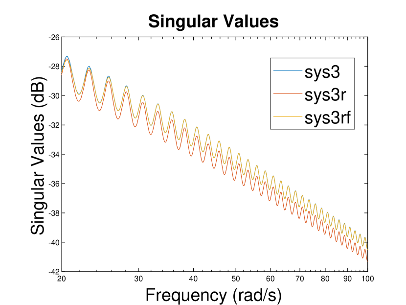
Figure 4: Reduced systems sys3r and sys3rf over $[20,\infty)$.

The zoomed version of the sigma plot, Figure 4, shows that the frequency-limited balanced reduction approximates better compared to the standard reduction over the focused frequency range.

As a final remark, the object info stores the gramian related information and the full balancing transformation matrices. The function balred computes the reduced orders very fast when info is provided since it does not recompute gramian information, i.e.,

>> tic; [sys3r,info3] = balred(sys3,2); time=toc
>> tic; sys3r1 = balred(sys3,4,info3); time=toc

time = 3.1990

time = 0.0041

5 Benchmark Problems

We surveyed the literature and collected two sets of benchmark problems for the model reduction and the $\mathcal{H}_{2}$ norm computation. We prepared two executable notebooks in which we define the benchmark problems and show how to use SSD on them in GitHub repository.

5.1 Model Reduction

There are five benchmark problems provided in the executable notebook, benchmarks_model_reduction.mlx. We used the model reduction functionality of SSD on the selected benchmarks:

1. The heated rod (HR$2$) Example in Michiels (2011a): A $100^{\textrm{th}}$-order model with a single delay derived from the discretization of heat equations describing the temperature in a rod controlled with distributed delayed feedback.

2. Mass-spring (MS) system in Saadvandi et al. (2012): A $1000^{\textrm{th}}$-order coupled mass-spring system with dampers and feedback controls with delays.

3. Platoon of eight vehicles (P$8$V) in Scarciotti et al. (2014): A $23^{\textrm{rd}}$-order model describing the problem of controlling a group of vehicles tightly spaced following a leader, all moving in longitudinal direction.

4. Example $1$ in Lordejani et al. (2020): A $6^{\textrm{th}}$-order synthetic model with one state and one output delay.

5. Second-order system with proportional damping example (SOSPD) in Jiang et al. (2019): A $2000^{\textrm{th}}$-order model with a single state delay.

Table 1 shows the state, output, input dimensions and the number of delays for all system matrices. Since the maximum delay may affect the complexity of the method, this information is included in the table.

The examples in Saadvandi et al. (2012) and Jiang et al. (2019) are second-order mechanical systems and the orders of their first-order equivalent models are twice of their dimensions. The benchmark problems are single-input-single-output (SISO) systems and mostly single state delay in the state equation is considered.

Ex.	Dimensions	# Delays	Max.
	($n$,$n_{y}$,$n_{u}$)	($m_{A}$,$m_{B}$,$m_{C}$,$m_{D}$)	Delay
HR$2$	$(100,1,1)$	$(1,0,0,0)$	$1$
MS	$(1000^{\dagger},1,1)$	$(1,0,0,0)$	$2$
P$8$V	$(23,1,1)$	$(1,0,0,0)$	$0.005$
Ex.$1$	$(6,1,1)$	$(1,0,1,0)$	$1.6$
SOSPD	$(2000^{\dagger},1,1)$	$(1,0,0,0)$	$1$

${\dagger}$ The dimension of the second-order system.

Table 1: Model reduction benchmark problems

A snapshot of the heated rod example from our notebook can be seen in Figure 6.

Figure 5: A snapshot of the heated rod example.

Figure 6: A snapshot of the hot shower example.

5.2 $\mathcal{H}_{2}$ Norm Computation

There are six benchmark problems for $\mathcal{H}_{2}$ norm computation collected in our notebook, benchmarks_h2norm.mlx:

1. The hot shower (HS) problem in Jarlebring et al. (2011), Ex.$1$: A first-order state-space model whose $\mathcal{H}_{2}$ norm can be computed analytically. Its delay can be set by the user.

2. Example $2.b$ in Jarlebring et al. (2011), Ex.$2$b: A $3^{\textrm{rd}}$-order synthetic model with two state delays.

3. Example $3$ in Jarlebring et al. (2011), Ex.$3$: A $9^{\textrm{th}}$-order model with two state-delays obtained from discretization of partial differential equations with delays.

4. The heat exchanger (HE) example in Michiels et al. (2019): A $5^{\textrm{th}}$-order model with seven delays for a heat exchanger for which the controller based on a combination of static state feedback and proportional integral control.

5. The heated rod (HR$2$) Example in Peeters et al. (2013): A $100^{\textrm{th}}$-order model with a single delay, same as the previous example in the model reduction benchmarks.

6. The heated rod (HR$4$) Example in Michiels et al. (2019): A $10000^{\textrm{th}}$-order model with a single delay, same as the previous example with larger size.

Ref.	Dimensions	# Delays	Max.
	($n$,$n_{y}$,$n_{u}$)	($m_{A}$,$m_{B}$,$m_{C}$,$m_{D}$)	Delay
HS	$(1,1,1)$	$(1,0,0,0)$	User-defined
Ex.$2$b	$(3,1,1)$	$(2,0,0,0)$	$1$
Ex.$3$	$(9,1,1)$	$(2,0,0,0)$	$3$
HE	$(5,1,5)$	$(7,0,0,0)$	$40$
HR$2$	$(100,1,1)$	$(1,0,0,0)$	$1$
HR$4$	$(10000,1,1)$	$(1,0,0,0)$	$1$

Table 2: $\mathcal{H}_{2}$ benchmark problems

Table 2 summarizes the dimensions and the number of delays for all system matrices. In general, the examples in the literature has one or two state delays and no delays at input and output matrices excluding $D$ matrices which must be zero for well-posedness of the norm. Most examples are SISO systems. Finally, we share a snapshot from the executable notebook for the hot shower example in Figure 6.

6 Computational Aspects

For experimental testing of the computational complexity of balanced reduction and $\mathcal{H}_{2}$ norm computation, we randomly generate delay systems with the following properties:

• Input and output sizes are $3$, $n_{y}=n_{u}=3$,

• There are $3$ delays, $m_{A}=m_{B}=m_{C}=3$,

• All delays are uniformly selected from $(0,1)$,

• All matrices are dense whose elements uniformly selected from $[-3,3]$ and in addition, $3I$ subtracted from $A_{0}$ matrix to make it stable.

• $D$ matrices are set to zero since they are not needed for $\mathcal{H}_{2}$ norm computation and balanced reduction.

We validated that the generated delay systems have rich dynamics. We measured the computation time of h2norm and gram (computing both gramians) functions since the latter function is the main computational bottleneck of balreal and balred. The number of states varies as $1-10$, $10-100$ by $10$ increments and $100-500$ for by $100$ increments (The upper bound is $400$ for model reduction). For each step, we created $5$ delay systems, computed the average of computational times and the standard deviation.

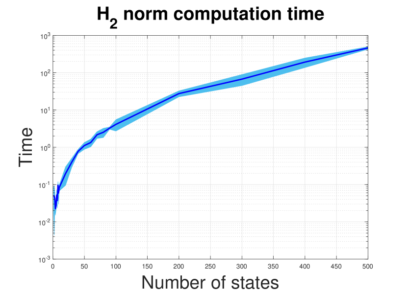
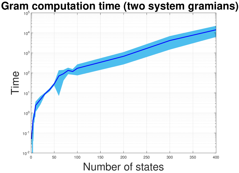
Figure 7: Average and standard deviation of the computation time of h2norm (left) and gram (right) functions with respect to the number of states.

Figure 7 (left) shows that the $\mathcal{H}_{2}$ norm computation time is in the order of seconds upto $100$ states, that of minutes upto $300$ states and around $8$ minutes for $500$ states.

Figure 7 (right) shows that the gram(sys,’co’) computation time is under a minute upto $50$ states, under $10$ minutes upto $200$ states and almost $2$ hours for $400$ states. In the light of these experiments, we see that SSD can handle small to medium size state dimensions.

For large-scale delay systems with sparse matrices, the sparse option of ssdoptions can be used to speed up the computation. As a large-scale benchmark, we computed the $\mathcal{H}_{2}$ norm of HR$4$ example with $10,000$ states from Section 5.2. We set the absolute tolerance a little high $10^{-3}$ to make the relative error active and set the relative error to $10^{-4}$ as reported in Michiels et al. (2019) and get similar order of time magnitude, around $6$ seconds, compared to their results $4.8$ seconds obtained by their special large-scale approach.

>> opt = ssdoptions(’Sparse’,true, ...
                    ’RelTol’,1e-4, ’AbsTol’,1e-3);
>> tic
>> h2 = h2norm(sys_hr4,opt)
>> time=toc

h2 = 0.4357

time = 5.9651

As a final remark, the function integral over $[0,\infty]$ interval may be computationally expensive or less accurate when the integrand has highly oscillatory behavior for a large part of the interval. In our experiments, it shows satisfactory performance.

7 Concluding Remarks

We took a guided tour of a new MATLAB package, SSD, on several examples. SSD seamlessly integrates with the time and frequency domain visualization capabilities of MATLAB while offering new features on model reduction and $\mathcal{H}_{2}$ norm computations built on a frequently-used RTDS delay system representation. The list of SSD functions is given in Table 3.

Focus	Function names
Visualizations	bode, bodemag, sigma, nyquist, step
Norm	h2norm†
Model Reduction	gram†, balreal, balred
Options	ssdoptions

${\dagger}$ Sparse computation is available.

Table 3: SSD functions

Our computational analysis shows that SSD is suitable for small to mid-size state dimensions. We hope that SSD’s delay system definition of matrices and delays, easy-to-use interface, and provided functionalities will facilitate the analysis of delay systems and be used as a baseline for advanced techniques.

All the examples in this paper are reproducible by our executable notebook, introduction.mlx. We share two executable notebooks, benchmarks_model_reduction.mlx and benchmarks_h2norm.mlx with a collection of benchmark problems on model reduction and $\mathcal{H}_{2}$ norm computation. SSD and three notebooks are available at the GitHub repo

https://github.com/gumussoysuat/ssd.

The author thanks Izmir D. Gumussoy for the fruitful discussions.

References

- Antoulas (2002) A. C. Antoulas. Approximation of Large-Scale Dynamical Systems. SIAM, 2005.
- Appeltans et al. (2019) P. Appeltans and W. Michiels. A pseudo-spectra based characterisation of the robust strong H-infinity norm of time-delay systems with real-valued and structured uncertainties. ArXiv, 1909.07778, 2019.
- Appeltans et al. (2022) P. Appeltans, S.-I. Niculescu, and W. Michiels. Analysis and Design of Strongly Stabilizing PID Controllers for Time-Delay Systems. SIAM J. Control Optim., 60:124-–146, 2022.
- Avanessoff et al. (2013) D. Avanessoff, A. R. Fioravanti, and C. Bonnet. YALTA: a Matlab toolbox for the -stability analysis of classical and fractional systems with commensurate delays. IFAC Proceedings Volumes, 46:839–844, 2013.
- Boussaada et al. (2021) I. Boussaada, G. Mazanti, S.-I. Niculescu, A. Leclerc, J. Raj, and M. Perraudin. New Features of P3 software: Partial Pole Placement via Delay Action. IFAC-PapersOnLine, 54:215–-221, 2021.
- Breda et al. (2009) D. Breda, S. Maset, and R. Vermiglio. TRACE-DDE: a Tool for Robust Analysis and Characteristic Equations for Delay Differential Equations. Topics in Time Delay Systems, Springer, 388:145–155, 2009.
- Breda et al. (2016) D. Breda, O. Diekmann, M. Gyllenberg, F. Scarabel and R. Vermiglio. Pseudospectral discretization of nonlinear delay equations: New prospects for numerical bifurcation analysis. SIAM J. Appl. Dyn. Syst., 15:1–23, 2016.
- Engelborghs et al. (2002) K. Engelborghs, T. Luzyanina, and D. Roose. Numerical bifurcation analysis of delay differential equations using DDE-BIFTOOL. ACM Transactions on Mathematical Software, 28:1–21, 2002.
- Enright et al. (1997) W. H. Enright and H. Hayashi. A delay differential equation solver based on a continuous Runge-Kutta method with defect control. Numerical Algorithms, 16:349–364, 1997.
- Gawronski et al. (1990) W. Gawronski and J.-N. Juang. Model reduction in limited time and frequency intervals. International Journal of Systems Science, 21:349–376, 1990.
- Gumussoy et al. (2010) S. Gumussoy and W. Michiels. A predictor–corrector type algorithm for the pseudospectral abscissa computation of time-delay systems. Automatica, 46:657–664, 2010.
- Gumussoy et al. (2011) S. Gumussoy and W. Michiels. Fixed-Order H-Infinity Control for Interconnected Systems Using Delay Differential Algebraic Equations. SIAM J. Control Optim, 49:2212–2238, 2011.
- Gumussoy et al. (2012) S. Gumussoy, B. Eryilmaz, and P. Gahinet. Working with Time-Delay Systems in MATLAB. IFAC Proceedings Volumes, 45:108–-113, 2012.
- Hairer et al. (1995) E. Hairer and G. Wanner. RETARD: Software for Delay Differential Equations. http://www.unige.ch/ hairer/software.html, 1995.
- Jarlebring et al. (2011) E. Jarlebring, J. Vanbiervliet, and W. Michiels. Characterizing and Computing the Norm of Time-Delay Systems by Solving the Delay Lyapunov Equation. IEEE Transactions on Automatic Control, 56:814–-825, 2011.
- Jarlebring et al. (2013) E. Jarlebring, T. Damm, and W. Michiels. Model reduction of time-delay systems using position balancing and delay Lyapunov equations. Math. Control Signals Syst., 25:147–-166, 2013.
- Jiang et al. (2019) Y.-L. Jiang, Z.-Y. Qiu, and P. Yang. Structure preserving model reduction of second-order time-delay systems via approximate Gramians. IET Circuits, Devices & Systems, 14:130–-136, 2019.
- Lordejani et al. (2020) S. Naderi Lordejani, B. Besselink, A. Chaillet, and N. van de Wouw. Model order reduction for linear time delay systems: A delay-dependent approach based on energy functionals. Automatica, 112:1–-10, 2020.
- Michiels et al. (2010) W. Michiels and S. Gumussoy. Characterization and computation of H-infinity norms of time-delay systems. SIAM Journal on Matrix Analysis and Applications, 31:2093–2115, 2010.
- Michiels (2011a) W. Michiels, E. Jarlebring, and K. Meerbergen. Krylov-Based Model Order Reduction of Time-delay Systems. SIAM J. Matrix Anal. Appl., 32:1399–-1421, 2011.
- Michiels (2011b) W. Michiels. Spectrum-based stability analysis and stabilisation of systems described by delay differential algebraic equations. IET Control Theory & Applications, 5:1829–-1842, 2011.
- Michiels et al. (2019) W. Michiels and B. Zhou. Computing Delay Lyapunov Matrices and Norms for Large-scale Problems. SIAM J. Matrix Anal. Appl., 40:845–-869, 2019.
- Peeters et al. (2013) J. Peeters and W. Michiels. Computing the H2 norm of large-scale time-delay systems. IFAC Proceedings Volumes, 46:114–-119, 2013.
- Saadvandi et al. (2012) M. Saadvandi, K. Meerbergen, and E. Jarlebring. On dominant poles and model reduction of second order time-delay systems. Applied Numerical Mathematics, 62:21–-34, 2012.
- Scarciotti et al. (2014) G. Scarciotti and A. Astolfi. Model Reduction by Moment Matching for Linear Time-Delay Systems. IFAC Proceedings Volumes, 47:9462–-9467, 2014.
- Shampine et al. (2001) L. F. Shampine and S. Thompson. Solving DDEs in Matlab. Applied Numerical Mathematics, 37:441–458, 2001.
- Vyhlidal et al. (2014) T. Vyhlídal, and P. Zítek. QPmR-Quasi-polynomial root-finder: Algorithm update and examples. Delay Systems, Springer, 1:299–312, 2014.
- Wu et al. (2012) Z. Wu and W. Michiels. Reliably computing all characteristic roots of delay differential equations in a given right half plane using a spectral method. Journal of Computational and Applied Mathematics, 236:2499–2514, 2012.