Ordinal analysis of lexical patterns

Abstract

Words are fundamental linguistic units that connect thoughts and things through meaning. However, words do not appear independently in a text sequence. The existence of syntactic rules induces correlations among neighboring words. Using an ordinal pattern approach, we present an analysis of lexical statistical connections for eleven major languages. We find that the diverse manners that languages utilize to express word relations give rise to unique pattern structural distributions. Furthermore, fluctuations of these pattern distributions for a given language can allow us to determine both the historical period when the text was written and its author. Taken together, our results emphasize the relevance of ordinal time series analysis in linguistic typology, historical linguistics and stylometry.

Natural languages are systems where complex relations are established between a huge number of words. This leads to a plentiful variety of forms that substantialize linguistic rules. Surprisingly enough, we find that a handful of ordinal patterns suffices to reliably characterize any language. Moreover, statistical fluctuations of these patterns can shed light on both date and authorship identification. Our method utilizes the sequential nature of language, which enables to map a sufficiently long text into a time series of word rankings.

I Introduction

Despite its complexity, language seems to be organized with a few structural principles Hauser, Chomsky, and Fitch (2002). For example, every language has a lexicon of thousands of words. These are basic elements with a particular meaning which can be combined in utterances to transmit a full idea. Although the potential number of combinations can be overwhelmingly large, a statistical analysis of lexical frequencies shows a scaling behavior (Zipf’s law Zipf (1935)) that establishes an inverse proportion with respect to word rankings. This probability distribution holds for large corpora and many different languages Piantadosi (2014) and has been linked to a cognitive principle of least effort in human communication Mandelbrot (1953); Ferrer i Cancho and Solé (2003).

Yet, the Zipf’s law yields no information on the selection rules that govern grammatical arrangements within a sentence. Indeed, words with the highest frequencies often operate with a purely syntactic purpose, such as determiners (e.g., the in English), prepositions (of), conjunctions (and) or pronouns (I), but unigram distributions like the Zipf’s law cannot provide insight into the deep relationships formed between function and content words to produce meaningful sentences. What is desirable, thus, is to investigate distributions of bigrams, trigrams, etc. Ha et al. (2009) to have a complete picture of the statistical patterns that underlie human language.

At first sight the task looks formidable. If $N$ is the vocabulary cardinality, the number of distinct $n$-grams is $N^{n}$. For a rough estimate of $N=10^{4}$, the possible combinations become exceedingly large already for $n=3$ and cannot hence be statistically analyzed with the largest available resources (e.g., the Google Books corpus Michel et al. (2011) includes around $10^{11}$ tokens). Even if one takes into account syntactic rules that forbid certain combinations, the number would continue to be enormous. Here, we take an approach that significantly simplifies the problem while revealing at the same time interesting linguistic patterns.

Our approach is based on an ordinal analysis Bandt and Pompe (2002); Zanin and Olivares (2021). A text is viewed as a time series where the time dimension corresponds to the discrete position of the word inside the text. This perspective is accurate because language is sequential in nature: one word comes after the other. Let us consider the beginning of the The Man Who Was Thursday, a 1908 novel by G. K. Chesterton: “A cloud was on the mind of men and wailing went the weather…". In Fig. 1 we plot the ranking of these words calculated from their absolute frequencies within the novel as a function of position. It follows that the is the top word type and appears at the bottom of the time series while content words (cloud, mind, men) possess a much lower occurrence and come into the high part of the time series. As a consequence, any text portion in the book consists of a succession of ups and downs as the story unfolds. Our aim is to study this ranking sequence rather than the particular ranking value as the Zipf’s law does. Below, we show that the distribution of increasing and decreasing patterns contains valuable information not only about the language itself but also about its history and the writer who generates the text. It is worth mentioning here that Sigaki et al. Sigaki, Perc, and Ribeiro (2018) have recently shown that physics-inspired measures estimated from ordinal patterns distributions, when plotted in a complexity-entropy plane, are able to capture relevant information about paintings, their style and their temporal evolution. Moreover, these measures can be consistently connected with qualitative canonical concepts proposed by art historians to distinguish artworks. Furthermore, the same bidimensional representation space, but just using unigram word frequencies for estimating information theory quantifiers, has previously been applied with success to characterize plays and poems by Shakespeare and other English Renaissance authorsRosso, Craig, and Moscato (2009). However, to the best of our knowledge, there has been no previous applications of ordinal analysis to texts. This is an interesting possibility that we explore in this work.

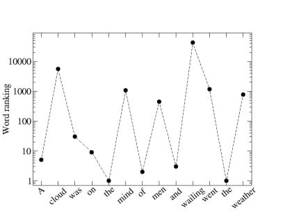
Figure 1: The text seen as a time series. The frequency count for the tokens that appear in The Man Who Was Thursday establishes a frequency ranking for all word types therein. For illustrative purposes, we show the beginning of the novel.

II Method

Let $W$ be the number of words in a given text. We rank its words according to their absolute frequency and convert the text into a sequence of rankings: $\mathcal{S}_{r}=\{r_{1},r_{2},\ldots,r_{W}\}$. This way, the $i$-th word in the sequence is replaced with its frequency ranking $r_{i}$. The rankings are calculated from each text separately. This guarantees that each word is assigned with a ranking. Another possibility is to use a common ranking for all works under consideration (see Appendix A), but our results are not significantly altered because $W$ is large for the texts considered in this work. A word of caution is necessary for rare words Tanaka-Ishii and Bunde (2016) since it may be that two words with very low frequency share the same ranking. Whenever this happens we randomly modify the rankings of the affected words to make sure that in $\mathcal{S}_{r}$ two neighboring terms are never equal. In Appendix B we give details of this procedure and prove that this modification does not affect the final results.

Our objective is to obtain the ordinal pattern distribution for the text. Depending on the embedding dimension $D$ in the time series Tsonis (1992) there exist $D!$ ordinal patterns. For instance, if $D=2$ as described above we have either an increasing or a decreasing pattern between two consecutive words with rankings $r_{i}<r_{i+1}$ in the first case and $r_{i+1}<r_{i}$ in the second case. We plot a sketch of these in the top-left panel of Fig. 2. Then, for the data in Fig. 1 the ordinal pattern sequence becomes $\mathcal{S}_{p}=\{1,2,2,2,1,2,1,2,1,2,2,1\}$, where we have assigned the symbols $1$ ($2$) to the increasing (decreasing) pattern. For $D=3$ we have six possibilities, namely, $1$ ($r_{i}<r_{i+1}<r_{i+2})$, $2$ ($r_{i}<r_{i+2}<r_{i+1}$), $3$ ($r_{i+1}<r_{i}<r_{i+2}$), $4$ ($r_{i+2}<r_{i}<r_{i+1}$), $5$ ($r_{i+1}<r_{i+2}<r_{i}$) and $6$ ($r_{i+2}<r_{i+1}<r_{i}$), see top-right panel in Fig. 2. As a result, the sequence in Fig. 1 can be symbolized as $\mathcal{S}_{p}=\{2,6,6,3,2,5,2,3,2,6,5\}$. The procedure can be straightforwardly generalized to higher embedding dimensions (see bottom panel in Fig. 2 for the 24 ordinal patterns with $D=4$).

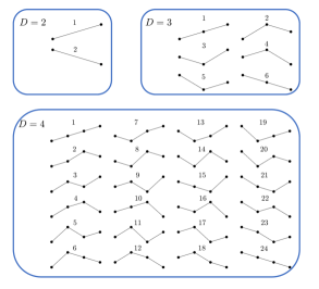
Figure 2: Ordinal patterns employed in this work. We take embedding dimensions $D=2$ (top left), $D=3$ (top right) and $D=4$ (bottom). Each dot represents a value in a word ranking diagram such as the one in Fig. 1.

Additionally, one may consider the embedding delay $\tau\in\mathbb{N}$ that defines the time separation between the elements Tsonis (1992). In the remainder of this paper, we take $\tau=1$, which implies consecutive data, thus fulfilling the sequential property of language. As a consequence, the embedding dimension agrees with the number of items in an $n$-gram. Another remark is in order. The pattern sequences $\mathcal{S}_{p}$ are generated allowing for overlaps between frequency rankings. Linguistically, this implies that our method probes the phrase structure of the sentence. This can be understood as follows. Quite generally, the pattern distributions show text correlations between segments of length $(D-1)\tau$. We have checked that for $\tau=3$ the results do not differ from a random sequence obtained by shuffling the text words. It follows that the method is sensitive to short-range correlations, unlike recent works that have paid attention to long-range correlations Schenkel, Zhang, and Zhang (1993); Ebeling and Pöschel (1994); Montemurro and Pury (2002); Altmann, Cristadoro, and Esposti (2012); Alvarez-Lacalle et al. (2006). These short-range correlations occur at the phrase (syntagmatic) level Montemurro and Pury (2002). Below, we provide further evidence for this.

We perform an analysis in three different levels. In the macroscale, we contrast the different ordinal pattern distributions across major language families Gordon (2005): Indo-European (English, Spanish, French, German, Latin and Russian), Afro-Asiatic (Somali), Niger-Congo (Xhosa), Turkic (Turkish), Austroasiatic (Vietnamese) and Austronesian (Tagalog). Our choice also allows for a broad variety of linguistic typologies. Since word order plays a crucial role in our findings (see Sec. III below), we focus on the most common subject-verb-object (SVO) arrangements found in human language: SVO (English, Spanish, French, Russian, Vietnamese, Xhosa), SOV (German, Latin, Somali, Turkish) and VSO (Tagalog), which amount to 96% of the existing typologies. We only exclude East Asian families (Sino-Tibetan, Japonic, Koreanic) because word boundaries are not clearly depicted in their written samples. However, the number of selected languages suffices to support our findings. To avoid possible differences due to the distinct nature of the analyzed texts and allow for a fair comparison, we need a single work, long enough, translated to the previously mentioned languages. The Bible fulfills all these requirements, is publicly available for natural language processing purposes Christodouloupoulos and Steedman (2015) and has already been employed in quantitative linguistics Mehri and Jamaati (2017).

In the mesoscale, we only consider one language (English) and examine its ordinal pattern distribution over time. For definiteness, we bring our attention to the four periods into which scholars traditionally divide the history of English: Old English, Middle English, Early Modern English and Modern English Sampson (1970). We pick representative works for each period (see Table 2 in Appendix C).

Finally, the microscale is concerned with individual authors. We fix both the language and the period (Modern English) and analyze a literary corpus gut (2021) corresponding to four writers: G. K. Chesterton, A. C. Doyle, H. P. Lovecraft and E. A. Poe. Notice that the two most important varieties of English (British and American) are equally represented with these authors. In Table 2 of Appendix C, we quote the five book titles for each of these writers employed for our microscale analysis.

All texts are tokenized using standard natural language processing toolkits Bird, Klein, and Loper (2009). This way, word forms are extracted and their rankings are straightforwardly calculated. We neglect lemmatization because this affects a small amount of word types and because Zipf’s law is preserved for lemmas Corral, Boleda, and Ferrer-i Cancho (2015). Hence, we do not expect significant changes in the results.

III Results

III.1 Macroscale level

We start our analysis by showing with blue curves in Fig. 3 the normalized frequencies of the $D=2$ pattern 1 for the different Bibles. (The frequency for the pattern 2 can be simply derived from probability normalization.) Each frequency is calculated for a temporal window of $10^{4}$ words. Then, the window is shifted $10^{3}$ time units until the book finishes. For all languages, the signals appear stochastic but clearly differ from a random sequence obtained by shuffling all the words (red curves). In the latter case, the series also fluctuate but their mean is $0.5$ as should be. In contrast, the expectation value for the original text is above or below $0.5$, depending on the language, suggesting that the stationary probabilities contain correlations entirely due to the word ordering dictated by the syntactic rules that operate in each human language. Note that we depict two sequences for German, each corresponding to a different Bible translation, showing that their dynamical behavior do not show significant changes.

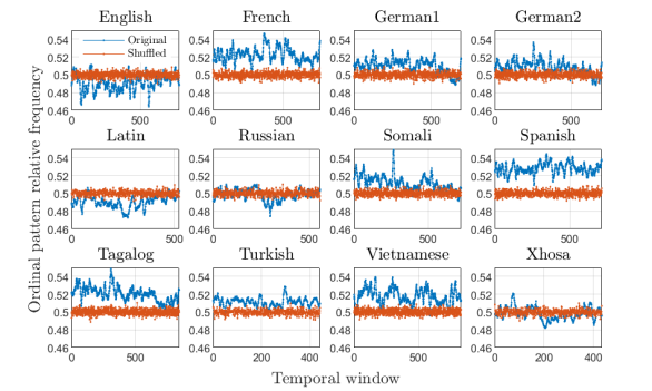
Figure 3: Relative frequency as a function of the text position for the Bible and the languages indicated above. We take pattern 1 as defined in Fig. 2 for embedding dimension $D=2$. Each frequency is calculated for a temporal window of $10^{4}$ words. Then, the window is shifted $10^{3}$ time units until the text finishes. Labels in the horizontal axis indicate the different, consecutive, window series. Whereas the blue curves correspond to the original text, the red dots indicate a shuffled (random) realization generated by randomly varying the token positions.

We now compare in Fig. 4 (blue curves) the probability distributions for the observed stationary ordinal patterns. Here, we choose a representative value for $D$ ($D=4$ but the same conclusion is achieved for any other value provided that $D!\ll W$). Quite remarkably, we find that every language has its own fingerprint. Admittedly, a few languages display similar histograms, such as French and Spanish (both Romance languages), but this should not make us think that the distributions are determined by the linguistic family. For instance, English and German are both Germanic languages and show distinct probability functions. On the other hand, Xhosa (and possibly Turkish) shows a uniform distribution close to the shuffled case, the latter shown as a red band with $3\sigma$ limits obtained after $100$ independent realizations. This diversity of possible ordering of the time series under analysis can be quantified with the permutation entropy (PE in the insets of Fig. 4), which is defined as the Shannon entropy of the ordinal pattern probability distribution. PE is the most representative and widely used ordinal descriptor. As seen, PE is essentially 1 for Xhosa and Turkish while the other languages show deviations form the uniform distribution. We attribute this result to the fact that Xhosa is a strongly agglutinative language where articles and prepositions are not typically independent words but morphemes that join to root words. We further discuss this particular effect in Appendix B. We also note that the results shown in Figs. 4 are not altered if the text sentences are shuffled, which is another proof that our ordinal approach only detects short-range correlations that typically occur among words inside a sentence (see Appendix D for a more detailed discussion). Finally, we do not observe any connection between the SVO order and the pattern probabilities. The linguistic reason underlying the divergences must be sought for somewhere else.

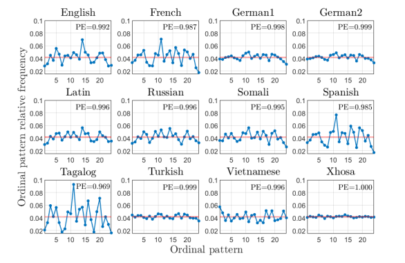
Figure 4: Macroscale results. We calculate pattern probability distributions at $D=4$ for the Bible in the indicated languages. In the $x$-axis we label the $D!=24$ possible patterns ordered as indicated in Fig. 2. Similarly to Fig. 3, the blue dots correspond to the original texts while the red curves show results for an ensemble of 100 shuffled realizations. Normalized permutation entropy (PE) estimated values are also included in each panel.

To gain further insight, we include in Table 1 the most frequent bigrams and their $D=2$ associated pattern for both English (top) and Spanish (bottom). Whereas in English the pattern 2 is more common, in Spanish the pattern with the highest probability is 1. What is the rationale for this difference? If we examine the top bigrams we find that their parsing is preposition + determiner (of the in English or de la in Spanish) or determiner + noun (the Lord in English or la tierra in Spanish). Therefore, their deep structures (in the generative grammar language sense Crystal (1997)) do not differ. It is instead the surface structure that determines the mean values for each pattern. Since the is the top word type in English, we find more instances of pattern 2 corresponding to the group preposition + determiner. Contrarily, this structure is built in Spanish with the preposition de, which is the top word type in this language and, as a consequence, pattern 1 appears more often. It is therefore not surprising that, as compared with Spanish, we derive an almost equal distribution in French, which employ similar words for these functions and with similar frequencies. Thus, the concrete pattern distributions are not only caused by the syntactic rules but also by the diverse strategies that languages employ to express these rules with the vocabulary at their disposal. This does not preclude the existence of linguistic universals Greenberg (1963); Montemurro and Zanette (2011) but these are not captured within our method.

Table 1: Bigrams with the largest frequencies. We consider both the English (top) and Spanish (bottom) Bibles. We also include their $D=2$ ordinal pattern as labeled in Fig. 2.

Bigram	Counts	Pattern
of the	11545	2
the lord	7036	1
and the	6278	2
in the	5031	2
and he	2794	1

(a)

Bigram	Counts	Pattern
de la	4250	1
de los	3966	1
en el	2494	2
a los	2331	1
la tierra	2202	1

(b)

III.2 Mesoscale level

Let us now discuss the mesoscale level. It is well known that language changes with time. Then, we expect that pattern distributions will evolve along history. We illustrate this phenomenon in Fig. 5. We take representative works for each historical period. In the Old English case [Fig. 5a)], we plot the probability distribution function for the following works: Andreas (curve 1), Anglo-Saxon Chronicle (2), Beowulf (3), Christ (4), Genesis (5) and Guthlac (6). Despite the fact that these texts are quite short, the distributions appear similar (with fluctuations due to the different lengths and genre). For the Middle English [Fig. 5b)] we use Layamon’s Brut (to have texts of similar lengths we split this work in curves 7 and 8), Canterbury Tales (9, 10 and 11), Confession Amantis (12, 13 and 14), Book of the Knight of La Tour-Landry (15) and Mandeville’s Travels (16). It is interesting to see the evolution in the patterns from the Old [Fig. 5a)] to the Middle periods [Fig. 5b)]. The latter distributions appear more similar because of both the smaller time range of their period and a higher language standardization, a process that began in the Late Middle Ages. The Early-Modern English corpus [Fig. 5c)] comprises works of Ben Jonson and those of Christopher Marlowe, Milton’s Paradise Lost, and Shakespeare’s Tragedies and Comedies (see Table 2 in Appendix C for their number identification). Finally, those chosen authors living in the Modern English period [Fig. 5d)] were previously mentioned and their numbering are also included in Table 2 in Appendix C. Clearly, there is an overall coherence among patterns belonging to the same time, which suggests that the traditional classification in periods has a lexical support.

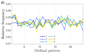
(a)

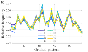
(b)

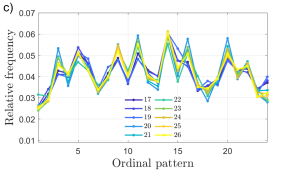
(c)

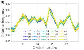
(d)

Figure 5: Mesoscale results. We show the ordinal pattern probability distribution for embedding dimension $D=4$ and different historical periods: a) Old English, b) Middle English, c) Early-Modern English and d) Modern English. Each curve corresponds to a single work or collection of works as listed in Table 2 of Appendix C. In the $x$-axis we label the $D!=24$ possible patterns ordered as indicated in Fig. 2.

This is better seen when one calculates the permutation Jensen-Shannon distance Zunino et al. (2022) between distributions and plots this distance for $D=4$ as in Fig. 6. As compared with the permutation entropy employed earlier in this work, the permutation Jensen-Shannon distance is more efficient to detect small differences between probability distributions. Remarkably, we observe four dark areas that correspond to the four historical periods, indicated with red lines. The distinction is clear between Old, Modern and the cluster formed by Middle English and Early-Modern English, between which the transition is less clear. This is because the Early-Modern English spans a period between the Renaissance, when the medieval forms were still popular, and the 17th century, when English conventions were approaching those of the Modern period. Interestingly, there exist individual deviations from the historical pattern. For instance, Anglo-Saxon Chronicle (work 2) appears to be close to the Middle English cluster whereas Paradise Lost (work 22) would be more suitable to be classified in the previous stage (Middle English), probably due to Milton’s intentionally archaic style. Another exception is Jonson (works 17, 18 and 19), whose style is better categorized within the Modern period. We highlight that despite the method’s simplicity we are not only able to correctly place literary works in their composition period but also detect singular departures assignable to particular style features.

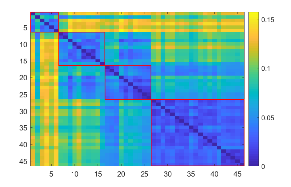
Figure 6: Permutation Jensen-Shannon distance for the mesoscale level. The distance is determined between pairwise probability distributions shown in Fig. 5 for $D=4$. Darker (lighter) colors indicate a small (large) distance, which quantifies the lexical (in the ordinal analysis language) difference among literary works belonging to distinct English historical periods. Red lines are included to help guide the eye.

III.3 Microscale level

Previous results are encouraging because they show that on top of a common background which characterizes written works in a given language there may exist fluctuations large enough that allow us to determine the author of a set of texts. In fact, a few subclusters with smaller distances can be distinguished in Fig. 6 for works of the same writers. This is particularly evident for Layamon’s, Gower’s, Jonson’s and Shakespeare’s works. We now pursue this idea by further analyzing the last historical period (microscale). In Fig. 7 we depict the ordinal patterns and their probability frequencies for $D=4$. Fluctuations are seen in the slight differences within the histogram. Then, we assess the pairwise distribution distance and plot the resulting matrix in Fig. 8. To obtain a more efficient discrimination between the texts, thus amplifying the fluctuations shown in Fig. 7, we set the embedding dimension to $D=6$, which allows for 720 patterns. Strikingly, we observe in Fig. 8 that each writer forms a cluster of his own, indicated with red lines. The largest distance takes place between Poe (works numbered between 16 and 20) and the rest, perhaps due to Poe’s highly mixed style. Here, we add an important caveat: the microscale is the most sensitive situation and Fig. 8 is only a proof of concept. To use this technique in author attribution tasks Grieve (2007) would require better refined analyses that fall beyond the scope of the present work.

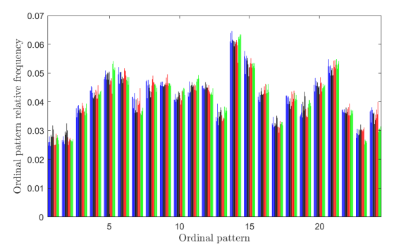
Figure 7: Microscale results. Histograms showing $D=4$ pattern probability distributions for four different authors from the same historical period (Modern English): G. K. Chesterton (blue), A. C. Doyle (black), H. P. Lovecraft (red) and E. A. Poe (green). On average the distributions are similar with fluctuations caused by author stylistic differences.

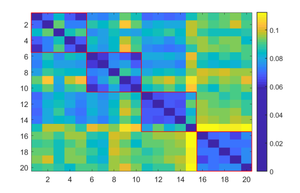
Figure 8: Permutation Jensen-Shannon distance for the microscale level. We determine the distance between the $D=6$ pattern probability distributions for the works of four English Modern authors (Chesterton, Conan Doyle, Lovecraft and Poe). The axes correspond to the numerical identification in parentheses of Table 2 of Appendix C. Red lines are included to help guide the eye.

IV Conclusion

To sum up, we have shown that the analysis of ordinal patterns is a powerful method that permits to distinguish (i) language, (ii) historical period and (iii) single authors. First, every language has a characteristic fingerprint in terms of a statistical distribution for symbolic patterns. The observed patterns emerge from a combination of the syntactic rules that shape each language and the way that this language articulates those rules. Second, a careful view of the pattern distribution provides useful information on the historical period when the text was produced. Third, since patterns have their origin in the greatly diverse procedures with which human languages embody the syntactic relations that constrain word combinations, the distributions show fluctuations that can be traced back to texts written by single authors.

The procedure discussed here has obvious limitations, the most important of which concerns semantics. Since every word is replaced with its ranking value in a table of frequencies, the symbolic patterns are agnostic with regard to meaning. However, this is the same limitation that takes place in all information-theoretic approaches to language since Shannon’s theory of communications Shannon (1951).

Our findings bode well for possible applications of our method. We envisage implementations in stylometry studies that seek a correct authorship attribution or in forensic linguistics for legal cases where linguistic data play a decisive role. Another interesting application would aim at the detection of speech impairments in individuals. Additionally, our idea could be useful within the sociolinguistics realm (characterization of dialects, registers and idiolects). An interesting avenue of future research would be to apply our method to spoken corpora and investigate whether there exist differences with the text corpora employed in this work.

Data Availability Statement

The data that support the findings of this study are openly available in Figshare at http://doi.org/10.6084/m9.figshare.21762947.v1.

Appendix A Common ranking

In this appendix, we calculate the ranking sequences differently. We consider a large corpus and arrange its words based on their occurrences. The corresponding rankings are then used to determine the ordinal patterns. The advantage of this approach is that all literary works are symbolized using the same ranking. The limitation is that word types that do not appear in the corpus cannot be assigned to a definite ranking and therefore not all patterns consist of consecutive words. However, we do not see a significant difference between both methods.

It suffices to illustrate this fact with a single language (e.g., English). We have checked that our conclusions are unaltered for different languages. The English word frequency list contains the 1/3 million most frequent words Norvig (2009) built from the Google Books Corpus (GBC) Lin et al. (2012). In Fig. 9a) we depict the symbol dynamics for $D=2$ obtained from the GBC ranking, comparing with the original series, which is reproduced in Fig. 9b) from the top left panel in Fig. 3. We find that the dynamical patterns resemble each other although the peak amplitudes differ. This is expected because the strength of the fluctuations depends on the word frequencies, which in turn are calculated from different corpora. However, the probability distributions are almost unaltered. We show this in Fig. 9c) for the GBC side by side with Fig. 9d), which is replicated from the top left panel in Fig. 4. This demonstrates the robustness of our method for alternative corpora provided that the size of the corpus is sufficiently large.

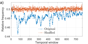
(a)

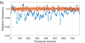
(b)

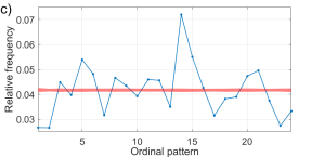
(c)

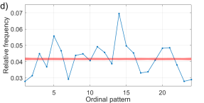
(d)

Figure 9: Dynamical behavior of the $D=2$ pattern 1 (blue curves) for the English Bible when the ranking sequences are generated by using a) a common and b) its own corpus. The corresponding ordinal pattern probability distributions for $D=4$ are displayed in c) and d), respectively. Results obtained when words are shuffled (red curves) are also included only for reference purposes. As in Sec. III.1, in the dynamical panels we only include a single shuffling realization to avoid finite size effects but in the distribution panels the red curves are indeed bands with $3\sigma$ limits calculated after 100 realizations.

Appendix B Sequences with equal rankings

If a sequence of $k$ words have the same ranking $r_{i}<r_{i+1}=r_{i+2}=\dots=r_{i+k}<r_{i+k+1}$, then we modify randomly those rankings by adding to each of $r_{i+1},\dots,r_{i+k}$ a uniform random number in the interval $(-(r_{i+1}-r_{i}),r_{i+k+1}-r_{i+k})$. Here, we provide evidence that our procedure of breaking ranking ties does not affect the main results except for a case that deserves attention. In Fig. 10 we plot with solid blue lines the pattern distributions when two words are allowed to have the same ranking. If this happens, equal rankings are sorted according to their temporal order. In addition, in Fig. 10 we reproduce with red dashed lines the case as in Fig. 4. Clearly, adding a small random number preserves the general structure of the probability distributions. The case where the two distributions seriously differ is Xhosa (and, to a smaller degree, Turkish). This is caused by the large number of word types that have occurrence 1 or 2 in the text. Therefore, it is likely that two consecutive words have the same ranking and adding a small random number is now not negligible. We ascribe this effect to the agglutinative nature of Xhosa. Unlike, e.g., English, which expresses most of its syntactic functions with isolated words, Xhosa displays agglutinated morphological complexes. It is thus natural to expect in the Xhosa Bible a large amount of hapax legomena. Any random shift will then represent a significant perturbation to the original series, as observed in our data.

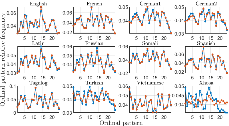
Figure 10: Distribution of linguistic ordinal patterns for embedding dimension $D=4$ for the original text sequences (blue lines) and when a small random number is added to break ranking equalities (dashed red lines).

Appendix C List of literary works

Table 2 shows the full list of literary works employed in the mesoscale and microscale analyses in Sec. III.

No.	Title	Author
1	Andreas	Anonymous
2	Anglo-Saxon Chronicle	Anonymous
3	Beowulf	Anonymous
4	Christ	Anonymous
5	Genesis	Anonymous
6	Guthlac	Anonymous
7	Brut I	Layamon
8	Brut II	Layamon
9	Canterbury I	Chaucer
10	Canterbury II	Chaucer
11	Canterbury III	Chaucer
12	Confessio Amantis I	Gower
13	Confessio Amantis II	Gower
14	Confessio Amantis III	Gower
15	The Book of the Knight of La Tour-Landry	Caxton
16	The Travels of Sir John Mandeville	Mandeville
17	Every Man in His Humor. The Poetaster	Jonson
18	Epicoene. Cynthia’s Revels	Jonson
19	Bartholomew Fair. The Alchemist	Jonson
20	Tamburlaine the Great. Hero and Leander	Marlowe
21	The Jew of Malta. The Massacre at Paris	Marlowe
22	Paradise Lost	Milton
23	Tragedies I	Shakespeare
24	Tragedies II	Shakespeare
25	Comedies I	Shakespeare
26	Comedies II	Shakespeare
27	The Innocence of Father Brown (1)	Chesterton
28	The Man Who Knew Too Much (2)	Chesterton
29	The Napoleon of Notting Hill (3)	Chesterton
30	The Man Who Was Thursday (4)	Chesterton
31	The Wisdom of Father Brown (5)	Chesterton
32	Memoirs of Sherlock Holmes (6)	Conan Doyle
33	The Return of Sherlock Holmes (7)	Conan Doyle
34	The Sign of Four (8)	Conan Doyle
35	The Hound of the Baskervilles (9)	Conan Doyle
36	The Adventures of Sherlock Holmes (10)	Conan Doyle
37	The Randolph Carter Stories (11)	Lovecraft
38	The Dream Cycle (12)	Lovecraft
39	Twenty-Nine Tales (13)	Lovecraft
40	Twenty-Nine Collaborative Stories (14)	Lovecraft et al.
41	At the Mountains of Madness (15)	Lovecraft
42	The Works of Edgar Allan Poe I (16)	Poe
43	The Works of Edgar Allan Poe II (17)	Poe
44	The Works of Edgar Allan Poe III (18)	Poe
45	The Works of Edgar Allan Poe IV (19)	Poe
46	The Works of Edgar Allan Poe V (20)	Poe

Table 2: Literary works considered in the mesoscale and microscale analyses. The numerical identification of the left column is used in the legends of Figs. 5 and the axes of Fig. 6 while the numbers in parentheses are employed for the axes of Fig. 8.

Appendix D Shuffled sentences

The shuffled realizations of Figs. 3, 4 and 9 are obtained by randomly shuffling all the words in the original text. A different shuffled realization puts the sentences in random order, instead of the individual words. Remarkably, our results obtained for shuffled sentences are the same as those obtained for the original sequences. For definiteness, we select four languages and plot in Fig. 11 both the original pattern dynamics for $D=2$ (blue dots), reproduced from Fig. 3, and the ordinal pattern when the sentences are shuffled (red dots). Obviously, the dynamics do not agree because the relative frequencies are calculated over time windows and these windows contain texts with totally different sentences in both cases. However, the stationary values and their probability distributions are not modified. This is shown in Fig. 12 for $D=4$, where one can note that there is exact match between the original Bible (blue lines as replicated from Fig. 4) and the Bible with shuffled sentences (red dots). Since the short memory encountered in our analysis is based on these statistical distributions, we can safely conclude that our method detects short-range correlations that typically occur inside a sentence.

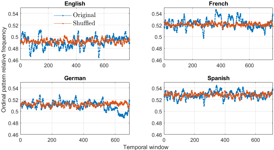
Figure 11: Dynamical behavior for $D=2$ as in Fig. 3 but comparing the original Bible (blue dots) and the Bible with shuffled sentences (red dots). In both cases, the curves differ from the case with shuffled words (the red curve in Fig. 3), which corresponds to the trivial dynamics.

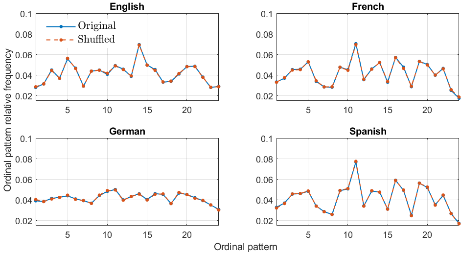
Figure 12: Pattern probability distributions for $D=4$ for the original Bible (blue lines as in Fig. 4) and the Bible with shuffled sentences (red dots).

References

- Hauser, Chomsky, and Fitch (2002) M. D. Hauser, N. Chomsky, and W. T. Fitch, “The faculty of language: What is it, who has it, and how did it evolve?” Science 298, 1569–1579 (2002).
- Zipf (1935) G. K. Zipf, The Psycho-biology of Language (Houghton-Mifflin, New York, NY, 1935).
- Piantadosi (2014) S. T. Piantadosi, “Zipf’s word frequency law in natural language: A critical review and future directions,” Psichon. Bull. Rev. 21, 1112–1130 (2014).
- Mandelbrot (1953) B. Mandelbrot, “On the theory of word frequencies and on related Markovian models of discourse,” in Structure of Language and its Mathematical Aspects, Vol. XII (1953) pp. 190–219.
- Ferrer i Cancho and Solé (2003) R. Ferrer i Cancho and R. V. Solé, “Least effort and the origins of scaling in human language,” Proceedings of the National Academy of Sciences 100, 788–791 (2003).
- Ha et al. (2009) L. Q. Ha, P. Hanna, J. Ming, and F. J. Smith, “Extending Zipf’s law to n-grams for large corpora,” Artificial Intelligence Review 32, 101–113 (2009).
- Michel et al. (2011) J.-B. Michel, Y. K. Shen, A. P. Aiden, A. Veres, M. K. Gray, T. G. B. Team, J. P. Pickett, D. Hoiberg, D. Clancy, P. Norvig, J. Orwant, S. Pinker, M. A. Nowak, and E. L. Aiden, “Quantitative analysis of culture using millions of digitized books,” Science 331, 176–182 (2011).
- Bandt and Pompe (2002) C. Bandt and B. Pompe, “Permutation entropy: A natural complexity measure for time series,” Phys. Rev. Lett. 88, 174102 (2002).
- Zanin and Olivares (2021) M. Zanin and F. Olivares, “Ordinal patterns-based methodologies for distinguishing chaos from noise in discrete time series,” Commun. Phys. 4, 190 (2021).
- Sigaki, Perc, and Ribeiro (2018) H. Y. D. Sigaki, M. Perc, and H. V. Ribeiro, “History of art paintings through the lens of entropy and complexity,” Proceedings of the National Academy of Sciences 115, E8585–E8594 (2018).
- Rosso, Craig, and Moscato (2009) O. A. Rosso, H. Craig, and P. Moscato, “Shakespeare and other English Renaissance authors as characterized by Information Theory complexity quantifiers,” Physica A 388, 916–926 (2009).
- Tanaka-Ishii and Bunde (2016) K. Tanaka-Ishii and A. Bunde, “Long-range memory in literary texts: On the universal clustering of the rare words,” PLOS ONE 11, e0164658 (2016).
- Tsonis (1992) A. A. Tsonis, Chaos: From Theory to Applications (Plenium Press, New York, NY, 1992).
- Schenkel, Zhang, and Zhang (1993) A. Schenkel, J. Zhang, and Y.-C. Zhang, “Long range correlations in human writings,” Fractals 1, 47–57 (1993).
- Ebeling and Pöschel (1994) W. Ebeling and T. Pöschel, “Entropy and long-range correlations in literary English,” EPL 26, 241–246 (1994).
- Montemurro and Pury (2002) M. A. Montemurro and P. A. Pury, “Long-range fractal correlations in literary corpora,” Fractals 10, 451–461 (2002).
- Altmann, Cristadoro, and Esposti (2012) E. G. Altmann, G. Cristadoro, and M. D. Esposti, “On the origin of long-range correlations in texts,” Proceedings of the National Academy of Sciences 109, 11582–11587 (2012).
- Alvarez-Lacalle et al. (2006) E. Alvarez-Lacalle, B. Dorow, J.-P. Eckmann, and E. Moses, “Hierarchical structures induce long-range dynamical correlations in written texts,” Proceedings of the National Academy of Sciences 103, 7956–7961 (2006).
- Gordon (2005) R. G. Gordon, Ethnologue. Languages of the World, 15th ed. (SIL International, Dallas, TX, 2005).
- Christodouloupoulos and Steedman (2015) C. Christodouloupoulos and M. Steedman, “A massively parallel corpus: the Bible in 100 languages,” Lang. Resources & Evaluation 49, 375–395 (2015).
- Mehri and Jamaati (2017) A. Mehri and M. Jamaati, “Variation of Zipf’s exponent in one hundred live languages: A study of the Holy Bible translations,” Physics Letters A 381, 2470–2477 (2017).
- Sampson (1970) G. Sampson, The Concise Cambridge History of English Literature, 3rd ed. (Cambridge University Press, Cambridge, UK, 1970).
- gut (2021) Project Gutenberg (Urbana, IL, 2021) https://www.gutenberg.org/.
- Bird, Klein, and Loper (2009) S. Bird, E. Klein, and E. Loper, Natural language processing with Python: analyzing text with the natural language toolkit (" O’Reilly Media, Inc.", 2009).
- Corral, Boleda, and Ferrer-i Cancho (2015) Á. Corral, G. Boleda, and R. Ferrer-i Cancho, “Zipf’s law for word frequencies: Word forms versus lemmas in long texts,” PloS one 10, e0129031 (2015).
- Crystal (1997) D. Crystal, The Cambridge Encyclopedia of Language, 2nd ed. (Cambridge University Press, Cambridge,UK, 1997).
- Greenberg (1963) J. H. Greenberg, “Some universals of grammar with particular reference to the order of meaningful elements,” in Universals of Language, Vol. 298, edited by J. H. Greenberg (MIT Press, 1963) pp. 73–113.
- Montemurro and Zanette (2011) M. A. Montemurro and D. H. Zanette, “Universal entropy of word ordering across linguistic families,” PLOS ONE 6, e19875 (2011).
- Zunino et al. (2022) L. Zunino, F. Olivares, H. V. Ribeiro, and O. A. Rosso, “Permutation Jensen-Shannon distance: A versatile and fast symbolic tool for complex time-series analysis,” Phys. Rev. E 105, 045310 (2022).
- Grieve (2007) J. Grieve, “Quantitative authorship attribution: An evaluation of techniques,” Literary and Linguistic Computing 22, 251–270 (2007).
- Shannon (1951) C. E. Shannon, “Prediction and entropy of printed English,” The Bell System Technical Journal 30, 50–64 (1951).
- Norvig (2009) P. Norvig, “Natural Language Corpus Data,” in Beautiful Data, edited by T. Segaran and J. Hammerbacher (O’Reilly Media, 2009) pp. 219–242.
- Lin et al. (2012) Y. Lin, J.-B. Michel, E. Lieberman Aiden, J. Orwant, W. Brockman, and S. Petrov, “Syntactic Annotations for the Google Books Ngram Corpus,” in Proceedings of the 50th Annual Meeting of the Association for Computational Linguistics (Association for Computational Linguistics, 2012) pp. 169–174.