Oscillating bound states in non-Markovian photonic lattices

Abstract

It is known that the superposition of two bound states in the continuum (BIC) leads to the phenomenon of an oscillating bound state, where excitations mediated by the continuum modes oscillate persistently. We perform exact calculations for the oscillating BICs in a 1D photonic lattice coupled to a “giant atom” at multiple points. Our work is significantly distinct from previous proposals of oscillating BICs in continuous waveguide systems due to the presence of a finite energy band contributing band-edge effects. In particular, we show that the bound states outside the energy band are detrimental to the oscillating BIC phenomenon, and can be suppressed by increasing either the number of coupling points or the separation between each coupling point. Crucially, non-Markovianity is necessary for the existence of oscillating BIC, and the oscillation amplitude increases with the characteristic delay time of the giant atom interactions. We also propose a novel initialization scheme in the BIC subspace. Our work be experimentally implemented on current photonic waveguide array platforms and opens up new prospects in utilizing reservoir engineering for the storage of quantum information in photonic lattices.

I Introduction

The study of interactions between atoms and photons traces its history all the way back to the inception of quantum mechanics itself. Since then, we have acquired a better understanding of atom-photon interactions which underpins the foundation of many quantum technologies such as atomic clocks Ludlow et al. (2015) and trapped-ion quantum computers and simulators Bruzewicz et al. (2019); Duan and Monroe (2010); Monroe et al. (2021), which harness the interaction of atoms with lasers. In many studies of atom-photon interactions, one often makes the dipole approximation Tannoudji et al. (1992), which assumes that the size of the atom is much smaller than the wavelength of the light. This is especially valid in optical regimes where the length scale of the atom $(\approx 10^{-10}\,\text{m})$ is orders of magnitude smaller than the wavelength of light $(\approx 10^{-7}\,\text{m})$. Under the dipole approximation, the time taken for the light to pass through a single atom is neglected, thus simplifying the interaction model. In the field of waveguide quantum electrodynamics (QED) Liao et al. (2016); Roy et al. (2017), which studies the interactions of atoms with a continuum of bosonic modes in a waveguide, the dipole approximation corresponds to modelling the atoms as coupled to individual points along the waveguide Shen and Fan (2005a, b). These atoms could either be actual atoms Bajcsy et al. (2009), or artificial atoms like quantum dots Akimov et al. (2007); Huck and Andersen (2016); Arcari et al. (2014) and superconducting qubits Astafiev et al. (2010a, b); Abdumalikov et al. (2010). A more complete overview of works done in this vein can be found in Chang et al. (2018); Gu et al. (2017); Sheremet et al. (2021).

However, this paradigm of dipole approximation in waveguide QED was recently broken with the discovery of the so-called “giant atoms” Frisk Kockum et al. (2014); Frisk Kockum (2021), by coupling each atom to two or more points on the waveguide. This was originally achieved by coupling the superconducting artificial atom (working in the microwave regime) to surface acoustic waves (SAW). Due to the low SAW velocity, for a given frequency the wavelength of sound is no longer assumed to be large compared to the size of the superconducting artificial atom. An alternative method to engineer giant atom coupling is by meandering the transmission line such that the atom interacts with the waveguide at multiple locations Kockum et al. (2018); Kannan et al. (2020). In these setups, we can no longer ignore the phase acquired by the light propagating in the 1D waveguide during the interaction with the giant atoms. Remarkably, by tuning the acquired phase Frisk Kockum et al. (2014), one obtains fascinating phenomena such as prolonged coherence time of a giant atom Frisk Kockum et al. (2014); Kannan et al. (2020), decoherence-free interactions between two giant atoms Kockum et al. (2018); Kannan et al. (2020) and the non-exponential decay of a giant atom Guo et al. (2017); Andersson et al. (2019), which have also been experimentally demonstrated in recent years.

Another novel feature of giant atoms in waveguide QED is the existence of oscillating bound states in the continuum (BIC), which is a genuine non-Markovian effect due to the significant time delay for information to propagate between the various coupling points of a giant atom Guo et al. (2017). The non-Markovianity manifests as a persistent oscillation of energy in the waveguide trapped between the coupling points of a giant atom, which behaves akin to a cavity. This is in stark contrast to the irreversible loss of energy from the giant atom to the waveguide in the Markovian regime. Thus, these oscillating BICs can potentially be harnessed to preserve quantum information in a non-Markovian bath by stabilizing the photonic quantum state, which we will show in this paper.

In the continuous waveguide case, it is usual to linearize the dispersion relation about the atom’s energy, since the coupling to the waveguide is weak Roy et al. (2017). The waveguide can then be regarded as having a linear dispersion with an infinite bandwidth. Instead of using a continuous waveguide such as a transmission line, we consider a 1D photonic lattice which acts as the reservoir for the giant atom. The key difference between the 1D photonic lattice that we consider here, and the continuous waveguide proposed in Guo et al. (2020), is the presence of a finite energy band where the band edge becomes significant, which restricts the allowed BICs. Experimentally, this can be achieved using a photonic waveguide array where each waveguide is side-coupled to each other via the evanescent field produced by the photon propagating inside the waveguides Jones (1965); Somekh et al. (1973). This has been proposed to simulate the non-exponential decay of a photonic giant atom Longhi (2020) which is simultaneously coupled to multiple lattice sites. We also note that while oscillating BICs have been reported in a discrete lattice system with two giant atoms Longhi (2021), manifesting as an effective Rabi oscillation between the atoms, the novelty of our work lies in only requiring a single giant atom to produce oscillating BICs.

As we will see, having a finite band gives rise to new conditions for the oscillating BIC phenomenon, which are distinct from those derived for the continuous waveguide. Moreover, we now need to consider the effect of bound states outside the energy band. These bound states outside the energy band are out of the continuum of allowed propagating modes and will henceforth be called bound states outside the continuum (BOC). As will be explained in more detail later, these BOCs are detrimental to quantum information storage as they are states with an exponentially-decaying wave function around the coupling points of the giant atom to the 1D photonic lattice. Hence, even though it is possible to observe oscillatory behavior in the emitter excitation probability with BOCs Ramos et al. (2016), we distinguish the oscillating BICs which we study here, which allow for perfect quantum information storage, from oscillations induced by BOCs which do not. We also show that the oscillating BIC is a consequence of the time-delayed interactions mediated by the 1D photonic lattice, and that a longer time delay generally results in a higher amplitude for the BIC which reduces the information leakage. A longer time delay also suppresses the unwanted contributions from the BOCs which hinder the ability of the GA to store and retrieve quantum information. This allows us to find the optimal conditions for oscillating BICs.

This paper is organized as follows: firstly, we introduce the model Hamiltonian and the theory behind BICs in Sec. II. Our main theoretical results are presented in Sec. III where we derive the new conditions for oscillating BICs in our system as well as optimal conditions to minimize the detrimental impact of BOCs. Thereafter, we present some numerical results in Sec. IV which support our analytical calculations. To demonstrate the feasibility of our theoretical results, we propose an experimental implementation of our work achievable on state-of-the art photonic hardware in Sec. V. Finally, we conclude in Sec. VI and provide several directions for future research.

II Theory

II.1 Model Hamiltonian

The Hamiltonian for the combined atom-lattice system can be written as $H=H_{a}+H_{\text{wg}}+H_{\text{int}}$, given in Eq. (1) as (setting $\hbar=1$)

$$H_{a} =\omega_{a}a^{\dagger}a+Ua^{{\dagger}2}a^{2}$$ (1a)

$$H_{\text{wg}} =J\sum_{n=1}^{N-1}(b_{n}^{\dagger}b_{n+1}+\text{H.c})$$ (1b)

$$H_{\text{int}} =\sum_{j=1}^{M}\rho_{j}(a^{\dagger}b_{n_{j}}+\text{H.c})$$ (1c)

where $a$ is the annihilation operator for the giant atom satisfying the bosonic commutation relation $[a,a^{\dagger}]=1$, and $b_{n}$ are the annihilation operators for the 1D photonic lattice with $[b_{n},b_{m}^{\dagger}]=\delta_{mn}$. $\omega_{a}$ is the detuning between the giant atom and the photonic lattice. The $N$ lattice sites are coupled to each other via a tight-binding Hamiltonian with interaction strength $J$. The giant atom is coupled to $M$ arbitrary lattice sites $\{n_{1},\ldots,n_{M}\}$ with strength $\rho_{j}$, $j=1,\ldots,M$. Here, $N$ is chosen to be a large number such that we can treat the lattice as an infinite 1D chain in both the left and right directions. The giant atom has an anharmonicity $U$, which we will take $U\to\infty$ such that it is equivalent to treating the giant atom as a two-level system. An illustration can be found in Fig. 1.

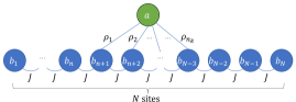
Figure 1: An illustration of the Hamiltonian in Eq. (1). Here, we have $N$ lattice sites arranged in a chain with bosonic annihilation operator $b_{n}$ for each lattice site. The $N$ lattice sites are described by a tight-binding Hamiltonian $H_{\text{wg}}$ with coupling strength $J$. We also have an extra lattice site described by the annihilation operator $a$ with Hamiltonian $H_{a}$, which we shall call the “giant atom” lattice site, due to its multiple coupling points to the 1D photonic lattice. The giant atom lattice site is coupled to the lattice sites $n_{1},n_{2},\dots n_{k}$ with coupling strengths $\rho_{1}$, $\rho_{2}$, $\dots$ $\rho_{n_{k}}$ respectively. This coupling is described by the Hamiltonian $H_{\text{int}}$.

As is shown in Appendix A, the Hamiltonian described by Eq. (1) can also be written in $k$-space in the first Brillouin zone as

$$H_{a} =\omega_{a}a^{\dagger}a$$ (2a)

$$H_{\text{wg}} =\int_{-\pi}^{\pi}dk\,\omega(k)c^{\dagger}(k)c(k)$$ (2b)

$$H_{\text{int}} =\int_{-\pi}^{\pi}dk\left\{G(k)a^{\dagger}c(k)+\text{H.c}\right\}$$ (2c)

by defining the $k$-space annihilation operators $c(k)$ through the discrete Fourier transform

$$c(k)=\frac{1}{\sqrt{2\pi}}\sum_{n=1}^{N}b_{n}e^{-ikn},\quad b_{n}=\frac{1}{\sqrt{2\pi}}\int_{-\pi}^{\pi}e^{ikn}c(k)\,dk.$$ (3)

The operators for the lattice $c(k)$ obey the bosonic commutation relations $\left[c(k),c^{\dagger}(k^{\prime})\right]=\delta(k-k^{\prime})$ with the dispersion relation $\omega(k)=2J\cos(k)$ and the spectral coupling function $G(k)=\frac{1}{\sqrt{2\pi}}\sum_{j=1}^{M}\rho_{j}e^{ikn_{j}}$. In general, $G(k)$ depends on the specific geometry of our system, such as the number of coupling points $M$ between the giant atom and the 1D photonic lattice and also the locations of the coupling points $n_{1},n_{2},\dots n_{M}$. In previous works Guo et al. (2017, 2020), the dispersion relation is linearized and the energy band formed by the waveguide modes is approximated to be infinite such that the band-edge effects become negligible. As we will see later, by confining the allowed energies to be in $[-2J,2J]$, we obtain new conditions for oscillating BICs. Before that, it is helpful to first review the essential physics of BIC in this system.

II.2 Bound states in the continuum

A system is said to have a bound state in the continuum (BIC) if there is an energy eigenstate with energy $\Omega$, where $\Omega$ lies in the band of allowed energies of the system. BICs are theoretically very interesting because conventionally, we would not expect a bound state to exist within a continuum of propagating states that would carry the energy of the bound state away, and yet these BICs truly exist and have been investigated both theoretically and experimentally Stillinger and Herrick (1975); Plotnik et al. (2011); Hsu et al. (2016); Longhi (2007). Specifically, for the setup that we are considering, the system has a BIC with energy $\Omega$ if $\Omega\in[-2J,2J]$ which is defined by the tight-binding dispersion relation $\omega(k)=2J\cos(k)$. Furthermore, for a BIC at energy $\Omega$ to exist, either the density of modes vanishes at $\omega=\Omega$ so that there is no mode in the continuum for the bound state to decay into, or the coupling to the continuum vanishes at $\omega=\Omega$. Lastly, since the BIC is a bound state by definition, we also require the energy eigenstate at frequency $\Omega$ to have a finite norm. The above conditions can be stated in more mathematically precise terms Longhi (2007).

Defining the density of modes $\rho(\omega)\equiv\frac{\partial k}{\partial\omega}$, the density of modes vanishing at $\omega=\Omega$ means that we require $\frac{\partial k}{\partial\omega}\bigr{|}_{\Omega}=0$, which is not possible for the tight-binding dispersion relation. Thus, by designing the giant atom coupling, we enforce the condition for the coupling to the continuum to vanish at $\Omega$

$$|G(k(\Omega))|^{2}=0.$$ (4)

If we restrict ourselves to the one-excitation subspace, a general time-dependent state of the system can be written as

$$|\psi(t)\rangle=\psi_{a}(t)|1_{a}\rangle+\int_{-\pi}^{\pi}dk\,\psi(k,t)|1_{k}\rangle$$ (5)

where $|1_{a}\rangle=a^{\dagger}|0\rangle$, $|1_{k}\rangle=c^{\dagger}(k)|0\rangle$. By considering an energy eigenstate $|E\rangle$ also in the one-excitation subspace, we obtain

$$\Omega-\omega_{a}=\int_{-\pi}^{\pi}dk\frac{|G(k)|^{2}}{\Omega-\omega(k)}$$ (6)

by comparing the coefficients of $|1_{a}\rangle$ and $|1_{k}\rangle$ in the energy eigenvalue equation $H|E\rangle=\Omega|E\rangle$. Hence, the requirement that we have an energy eigenstate with energy $\Omega$ within the band implies that the solution of Eq. (6) for $\Omega$ lies in the range $[-2J,2J]$. The preceding calculation also gives us an expression for the coefficient of $|1_{k}\rangle$, from which we can deduce that the finite norm requirement of the energy eigenstate is equivalent to $\rho(\omega)|G(k(\omega))|^{2}$ vanishing in the limit $\omega\to\Omega$ at least as fast as $\sim(\Omega-\omega)^{2}$. The integral in Eq. (6) can be evaluated by first evaluating the self-energy $\Sigma(s)$ defined by

$$\Sigma(s)=\int_{-\pi}^{\pi}dk\,\frac{|G(k)|^{2}}{is-\omega(k)}.$$ (7)

from which we get

$$\Omega-\omega_{a}=\text{Re}[\Sigma(s=-i\Omega\pm 0^{+})].$$ (8)

A detailed derivation of the above equations is presented in Appendix B.

II.3 Decay dynamics

In order to probe the decay dynamics of the giant atom into the 1D photonic lattice, we initialize the system with one excitation in the giant atom and the lattice in the vacuum state. Mathematically, with reference to Eq. (5), we have $\psi_{a}(0)=1$ and $\psi(k,0)=0\,\forall k\in[-\pi,\pi]$. From the Schrödinger equation $i\partial_{t}|\psi(t)\rangle=H|\psi(t)\rangle$ with these initial conditions, it can be shown (see Appendix C) that $\Sigma(s)$ controls the time-dependent probability amplitude $\psi_{a}(t)$ through the equation

$$\psi_{a}(t)=\sum_{\text{All residues}}\frac{ie^{st}}{is-\omega_{a}-\Sigma(s)}.$$ (9)

From Eq. (9), we see that poles on the right-hand-side of the equation with a non-zero real component will lead to a decay in $\psi_{a}(t)$. On the other hand, for the poles on the right-hand-side of the equation that lie on the imaginary axis, i.e if $s=-i\Omega$, the exponential factor in the numerator will be $e^{-i\Omega t}$, which is non-decaying and physically represents a BIC arising from the giant atom decay. We note that (see Appendix B) when there exists an $\Omega$ that fulfils Eq. (8) as well as $|G(k(\Omega))|^{2}=0$, then $\Omega$ will be a pole on the imaginary axis, which means that we will have a BIC at the frequency $\Omega$.

These BICs arising from giant atom decay are very interesting because by construction they are immune to decay into the 1D lattice, and hence can be used in a manner analogous to the so-called “dark states” for purposes like storing quantum information etc Johnsson and Mølmer (2004); Yang et al. (2004). Denoting the BIC energies as $\Omega_{j}$, which satisfy both Eq. (8) and Eq. (4), with simple poles at $s=-i\Omega_{j}$, we have

$$\psi_{a}(t) =\sum_{j}\lim_{s\to-i\Omega_{j}}\left[\frac{ie^{st}}{is-\omega_{a}-\Sigma(s)}(s+i\Omega)\right]$$

$$=\sum_{j}\frac{e^{-i\Omega_{j}t}}{1+i\Sigma^{\prime}(-i\Omega_{j})}$$ (10)

where we used L’Hopital’s rule and also defined $\Sigma^{\prime}=\partial_{s}\Sigma$ to get to the second line. Moreover, by noting that

$$\psi_{a}(t)=\sum_{E}e^{-iEt}|\langle 1_{a}|E\rangle|^{2}$$ (11)

we obtain the emitter contribution of each BIC as

$$|\phi_{a}^{(j)}|^{2}\equiv|\langle 1_{a}|\Omega_{j}\rangle|^{2}=\frac{1}{1+i\Sigma^{\prime}(-i\Omega_{j})}$$ (12)

The usefulness of each of these BICs can be quantified by the magnitude of $|\phi_{a}^{(j)}|^{2}$, since a large $|\phi_{a}^{(j)}|^{2}$ implies that the giant atom has a high probability of being excited despite the existence of decay channels in the continuum for it to decay into.

III Oscillating bound states

Consider the case of giant atom decay in the one-excitation subspace again. From Eq. (9), if there exists two BICs at frequency $\Omega_{\alpha}$ and $\Omega_{\beta}$ that have relative large residues compared to the other BICs, we have $\psi_{a}(t)\approx Ae^{-i\Omega_{\alpha}t}+Be^{-i\Omega_{\beta}t}$ for some complex numbers $A$ and $B$. This means that the emitter probability $|\psi_{a}(t)|^{2}$ oscillates sinusoidally with frequency $|\Omega_{\alpha}-\Omega_{\beta}|/2\pi$. We can also infer the same fact by looking at Eq. (11). In this scenario, we say that our system exhibits an oscillating BIC. Interestingly, we will show that these oscillating BICs inherently require non-Markovianity in the system, resulting in a bath-induced stabilization of a single-photon quantum state which can be used both as a photon trapped in a cavity as well as a storage for quantum information. Ideally, we would want $|A|=|B|$ so that at some time $t$, we have $|\psi_{a}(t)|^{2}=0$ which means that by turning off the giant atom couplings to the 1D lattice chain at that time, we can release the stored photon into the 1D chain.

Let us now calculate the conditions in which the setup shown in Fig. 1 exhibits an oscillating BIC. Consider the case where the giant atom has $M$ coupling points equally spaced apart by $n_{0}$ sites on the photonic lattice. For $N$ lattice sites, let the giant atom be coupled to sites $0$, $n_{0}$, $2n_{0}$, $\dots$, $(M-1)n_{0}$ with a uniform coupling strength $\rho_{0}$. For this particular setup, we have

$$G(k)=\frac{\rho_{0}}{\sqrt{2\pi}}\sum_{j=0}^{M-1}e^{ijkn_{0}}$$ (13)

As shown in Appendix E, it is not possible for an oscillating BIC to exist when $M=2$, consistent with the results in a continuous linear waveguide Guo et al. (2020). Hence, we consider the case when $M\geq 3$ for which oscillating BICs exist. Detailed calculations can be found in Appendix D. We will summarize some of the key results here. We first calculate $|G(k)|^{2}$ to be

$$|G(k)|^{2}=\frac{\rho_{0}^{2}}{2\pi}\left(M+2\sum_{r=1}^{M-1}(M-r)\cos(kn_{0}r)\right)$$ (14)

which means that when we enforce Eq. (4) for the coupling to the continuum to vanish, we have

$$k=\frac{2\pi}{n_{0}}\left(m\pm\frac{1}{M}\right)$$ (15)

where $m\in\mathbb{Z}$. Furthermore, Eq. (7) and Eq. (14) together give us

$$\Sigma(s) =\frac{\mp i\rho_{0}^{2}}{\sqrt{s^{2}+4J^{2}}}\left[M+2\sum_{r=1}^{M-1}(M-r)\alpha^{rn0}\right]$$ (16)

$$\alpha =\left(\frac{\mp i\sqrt{s^{2}+4J^{2}}+is}{2J}\right)$$ (17)

where we have the negative sign in both $\alpha$ and $\Sigma(s)$ above when $\text{Re}(s)>0$ and the positive sign when $\text{Re}(s)<0$. Since the subsequent results are the same regardless of whether we consider $\text{Re}(s)>0$ or $\text{Re}(s)<0$, we will restrict ourselves to the $\text{Re}(s)>0$ case. Thereafter, from Eq. (8), Eq. (16) and Eq. (17) we have

$$\Omega-\omega_{a}=\frac{-i\rho_{0}^{2}}{\sqrt{4J^{2}-\Omega^{2}}}\left[M+2\sum_{r=1}^{M-1}(M-r)(e^{in_{0}\theta})^{r}\right]$$ (18)

where $\theta=\arctan(-\sqrt{4J^{2}-\Omega^{2}}/\Omega)$. Hence, to obtain an oscillating BIC, we need to solve Eq. (18) together with Eq. (15) to obtain two eigenenergies $\Omega_{1}$ and $\Omega_{2}$ such that the coupling to the continuum vanishes at these two energies.

At this juncture, we consider the case where $\omega_{a}=0$, such that the giant atom energy is positioned at the band center. This is done so that the BIC energies $\Omega_{1},\Omega_{2}$ are symmetric about the band center, i.e $\Omega_{1}=-\Omega_{2}$, which is necessary to obtain perfectly sinusoidal oscillations of the giant atom emitter probability. From Eq. (15), we see that $n_{0}$ being an odd number will not give us BIC energies that are symmetric about the band centre. Hence, $n_{0}$ is restricted to be an even number which give us two possibilities, $n_{0}=2(2l)$ or $n_{0}=2(2l+1)$ where $l\in\mathbb{Z}^{+}$. Since the giant atom energy is positioned at the band center, we would expect the BIC energies that are closer to the band center to correspond to states that have a larger emitter probability. Using that criteria, we find that the optimal condition for oscillating BIC occurs for the $n_{0}=4l$ case (see Appendix D) from which we get the BIC energies $\pm\Omega_{\text{BIC}}$ given by

$$\Omega_{\text{BIC}}=2J\sin\left(\frac{2\pi}{Mn_{0}}\right).$$ (19)

We can then obtain the corresponding $\rho_{0}$ for $\pm\Omega_{\text{BIC}}$ by substituting Eq. (19) into Eq. (18) together with $\omega_{a}=0$ to obtain

$$\left(\frac{\rho_{0}}{J}\right)^{2}=\frac{2}{M}\tan\left(\frac{\pi}{M}\right)\sin\left(\frac{4\pi}{Mn_{0}}\right)$$ (20)

resulting in an oscillating BIC at the frequency $\Omega_{\text{BIC}}/\pi$. Now we can obtain the emitter probabilities of each BIC by substituting Eq. (19) and Eq. (20) into Eq. (12) to obtain

$$|\phi_{a}^{(\text{BIC})}|^{2}\equiv\langle 1_{a}|\pm\Omega_{\text{BIC}}\rangle|^{2}=\frac{ie^{-\frac{4i\pi}{M}}\left(1+e^{\frac{2i\pi}{M}}\right)\left(-1+\left(ie^{\frac{2i\pi}{Mn_{0}}}\right)^{n_{0}}\right)^{3}\csc^{2}\left(\frac{\pi}{M}\right)\cos^{2}\left(\frac{2\pi}{Mn_{0}}\right)}{4\left(2n_{0}\sin\left(\frac{4\pi}{Mn_{0}}\right)+\sin\left(\frac{2\pi(n_{0}-2)}{Mn_{0}}\right)+\sin\left(\frac{2\pi(n_{0}+2)}{Mn_{0}}\right)\right)}$$ (21)

From the emitter probabilities obtained above, using Eq. (9) and Eq. (10), we see that in the long time limit after all the non-BIC states have propagated away from the giant atom to the left and right ends of the lattice chain, we would expect oscillations in the emitter probability of the giant atom with amplitude $(2|\phi_{a}^{(\text{BIC})}|^{2})^{2}$. From Eq. (21), we note that for all values of $n_{0}=4l,l\in\mathbb{Z^{+}}$, $|\phi_{a}^{(\text{BIC})}|^{2}$ increases monotonically with $M$, eventually saturating at the limiting value $|\phi_{a}^{(\text{BIC})}|^{2}=1/3$. Consequently, for any value of $n_{0}$, having a larger number of coupling points $M$ leads to higher-amplitude oscillating BICs. It is also helpful to use Eq. (21) to compute the asymptotic behavior of $|\phi_{a}^{(\text{BIC})}|^{2}$ as $n_{0}\to\infty$, which we can write as

$$|\phi_{a}^{(\text{BIC})}|^{2} =\frac{1}{1+\frac{4\pi}{M}\csc\left(\frac{2\pi}{M}\right)}+\frac{A}{n_{0}^{2}}+\mathcal{O}\left(\frac{1}{n_{0}^{4}}\right)$$ (22)

$$\text{where }A =\frac{4\pi^{2}\sin\left(\frac{2\pi}{M}\right)\left(3M\sin\left(\frac{2\pi}{M}\right)-4\pi\right)}{3M\left(M\sin\left(\frac{2\pi}{M}\right)+4\pi\right)^{2}}.$$

By defining $\tau=(Mn_{0})/\nu_{g}$ as the time taken for the photon to propagate between the first coupling point and the $M$th coupling point (i.e, the size of the giant atom), where $\nu_{g}=2J$ is the group velocity at the band centre, and $\Gamma^{-1}=(M^{2}\rho_{0}^{2}/J)^{-1}$ as the characteristic timescale for the giant atom decay, we can quantify the amount of non-Markovianity in our system through the quantity $\tau/\Gamma^{-1}$ which can be written as

$$\frac{\tau}{\Gamma^{-1}} =M^{2}n_{0}\sin\left(\frac{4\pi}{Mn_{0}}\right)\tan\left(\frac{\pi}{M}\right)$$ (23)

$$=4M\pi\tan\left(\frac{\pi}{M}\right)-\frac{32\left(\pi^{3}\tan\left(\frac{\pi}{M}\right)\right)}{3M}\frac{1}{n_{0}^{2}}+\mathcal{O}\left(\frac{1}{n_{0}^{4}}\right)$$ (24)

where to get from the first line to the second line, we computed the asymptotic behavior as $n_{0}\to\infty$. From Eq. (24), we see that at large $n_{0}$ the non-Markovianity in our system, which has the same $1/n_{0}^{2}$ scaling as the expressions for the BIC emitter probabilities in Eq. (22). This allows us to conclude that a stronger non-Markovianity in our system arising from the time delay for information to propagate between the giant atom coupling points results in better oscillating BICs, though the amount of non-Markovianity quantified by $\tau/\Gamma^{-1}$ eventually reaches a plateau. The presence of the plateau means that even though $\tau$ increases as $n_{0}$ increases, which leads to a greater non-Markovianity in the system, this effect is quickly balanced by an increase in the giant atom lifetime $\Gamma^{-1}$ which is a result of a decreased coupling strength $\rho_{0}$. In practice, $n_{0}$ should of course not be too large since the oscillation period scales as $\sim n_{0}$ which might lead to more decoherence. Fortunately, the fast convergence $\mathcal{O}(1/n_{0}^{2})$ of the emitter probabilities means that a moderate $n_{0}$ is already sufficient to observe good oscillating BICs.

Finally, we note that for all values of $n_{0}=4l,l\in\mathbb{Z}^{+}$, as $M\to\infty$, $\tau/\Gamma^{-1}$ monotonically decreases to a limiting value of $4\pi^{2}$. This implies that our system with an oscillating BIC is inherently non-Markovian in nature, since there is a non-negligible lower bound to $\tau/\Gamma^{-1}$.

III.1 Role of imperfections: Bound states outside the continuum

Bound states outside the continuum (BOCs) are energy eigenstates of the Hamiltonian that have energy out of the range $[-2J,2J]$. For these states, the wave number $k$ is complex Munro et al. (2017), which means that these states are unable to propagate in the 1D lattice chain and hence they have a significant probability amplitude in $|1_{a}\rangle$, with an exponentially-decaying wavefunction around the coupling points of the giant atom. These states are imperfections to our oscillating BIC for two reasons. Firstly, for an oscillating BIC produced by giant atom decay, we want the emitter probability to be high for the two BICs involved at $\pm\Omega_{\text{BIC}}$, and low for all the other energy eigenstates. Yet these BOCs have a large atomic component and hence they act as imperfections to our sinusoidal oscillation as per Eq. (9). Secondly, these states leak energy outside the giant-atom coupling points due to the exponential decay of the photon amplitude from the coupling points.

To characterize the effect of BOCs on oscillating BIC produced by giant atom decay, we first use Eq. (20) to obtain $\rho_{0}$ corresponding to the oscillating BIC condition. Then, we solve for the BOC energies $\Omega_{\text{BOC}}$ where $|\Omega_{\text{BOC}}|>2J$ in Eq. (6) with $\omega_{a}=0$. In the limit of $n_{0}\to\infty$, the two BOC energies can be found as

$$\Omega_{\text{BOC}}\approx\pm 2J\left(1+\frac{2\pi^{2}\tan(\pi/M)^{2}}{M^{2}n_{0}^{2}}\right)$$ (25)

with the emitter probability

$$\left|\phi_{a}^{(\text{BOC})}\right|^{2}\sim\frac{4\pi^{2}\tan(\pi/M)^{2}}{M^{2}}\frac{1}{n_{0}^{2}}.$$ (26)

This means that for a given value of $M$, at large $n_{0}$, the contributions from the BOCs to the oscillations are suppressed by a factor of $1/n_{0}^{2}$. By comparing Eq. (26) and Eq. (24), we see that a larger non-Markovianity in our system characterized by a larger $\tau/\Gamma^{-1}$ leads to reduced imperfections from the BOC. We also note that having a larger number of coupling points $M$ leads to a diminished effect of the BOCs on our oscillating bound states, which can be explained by how a larger value of $M$ leads to a smaller coupling $\rho_{0}$ between the giant atom and the lattice chain.

III.2 Initialization in the BIC subspace

Up till now, we have considered the case of giant atom decay into the 1D lattice chain. If instead we are given the ability to initialize the state of the lattice sites in the chain, which is possible for some experimental platforms such as a side-coupled waveguide array through pulse shaping techniques, we can eliminate the effects of the BOCs even at low $n_{0}$ and also obtain perfect storage of quantum information within the legs of the giant atom. This is especially important for small values of $M$ like $M=3$, since from Eq. (26) we see that the emitter probability of the BOC states increases as $M$ decreases. Hence, we shall temporarily restrict ourselves to $M=3$ here, though it should be clear that the method below generalizes for any positive integer values of $M$.

We first write the states corresponding to the BICs at $\pm\Omega_{\text{BIC}}$ as

$$|\pm\rangle=\phi_{a,\pm}|1_{a}\rangle+\sum_{n}\phi_{n,\pm}|n\rangle.$$ (27)

Without loss of generality, we can set $\phi_{a,\pm}=|\phi_{a}^{(\text{BIC})}|$ since eigenstates are defined up to a global phase. Here $\phi_{n,\pm}$ are the photon amplitudes in real space, which for $M=3$ we can calculate $\phi_{n,\pm}$ to be given by

$$\phi_{n,+}=C\times\begin{cases}\begin{aligned} &(-1)^{n}\exp{\left(i\frac{2\pi n}{3n_{0}}\right)}\\ &-\exp{\left(-i\frac{2\pi n}{3n_{0}}\right)},0\leq n\leq n_{0}\\ &(-1)^{n+1}\exp{\left(i\frac{2\pi}{3}\left(\frac{n}{n_{0}}-2\right)\right)}\\ &+\exp{\left(-i\frac{2\pi}{3}\left(\frac{n}{n_{0}}-2\right)\right)},n_{0}\leq n\leq 2n_{0}\\ &0,\quad\text{else}\end{aligned}\end{cases}$$ (28)

where

$$C=\frac{-i^{n+1}\phi_{a}\rho_{0}}{2J\cos\left(\frac{2\pi}{3n_{0}}\right)}$$ (29)

and $\phi_{n,-}=(-1)^{n+1}\phi_{n,+}^{*}$. The above calculation also means that the state

$$|p\rangle \equiv\frac{1}{\sqrt{2}}(|+\rangle-|-\rangle)$$

$$=\frac{1}{\sqrt{2}}\sum_{n}\left(\phi_{n,+}-\phi_{n,-}\right)|n\rangle$$ (30)

is a state with no probability amplitude in $|1_{a}\rangle$ and with photon amplitudes in real space only within the $M$ coupling points of the giant atom. Thus if we initialize the state in $|p\rangle$, then there will be zero excitation leakage outside of the giant atom and the lattice sites within the $M$ coupling points. Furthermore, since the states $|\pm\rangle$ are orthogonal to the BOCs, the imperfections in the oscillations due to the BOCs are eliminated by construction. Lastly, we note that for $M=3$ the photon amplitudes are real and only differ in phase by $0$ or $\pi$, which makes it more feasible for practical implementation.

IV Numerical results

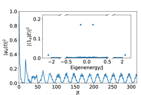
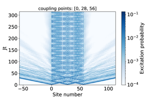
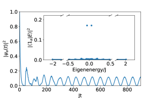
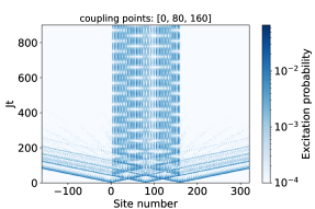
 (a)  (b)
 (c)  (d)

Figure 2: Simulation results for giant atom decay into the 1D photonic lattice for the case of $M=3$ coupling points. The coupling strength $\rho_{0}$ between the giant atom and the 1D photonic lattice can be calculated from Eq. (20). In (a) and (c) we have the excitation probability against time for the giant atom lattice site for $n_{0}=28$ and $n_{0}=80$ respectively. In the insets, we plot the emitter probability for each of the eigenstates of $H$. As can be seen in the insets, there are two eigenstates with energies in the continuum $[-2J,2J]$ that are symmetrical about $0$ and have a emitter probability. In (b) and (d) we have the excitation probability against time for some of the lattice sites in the 1D photonic lattice for $n_{0}=28$ and $n_{0}=80$ respectively. Initially we see some transient behavior as the non-bound states decay into the 1D lattice chain and are propagated away to the left and right ends of the 1D photonic lattice. Thereafter, we see the photon being trapped in between the $M=3$ coupling points with non-zero probability and oscillating between these three points with time. By comparing (a) and (c), we see that the $n_{0}=28$ case has oscillations that aren’t perfectly sinusoidal, due to the effect of the relatively large BOC emitter probabilities, as can be seen in the inset of (a). As was previously explained and is seen here in (b), the presence of these BOCs with large emitter probabilities for the $n_{0}=28$ case also lead to a leakage of the photon excitation probability beyond the coupling points of the giant atom. We can also see that this imperfection is absent for the $n_{0}=80$ case.

Here we first present in Fig. 2 some results for the $M=3$ giant atom decay coupled to a 1D photonic lattice with various values of $n_{0}$. For $M=3$, starting with a single excitation in the giant atom, in the absence of imperfections due to the BOCs, we should expect sinusoidal oscillations in the excitation probability of the giant atom lattice site with oscillation amplitude $(2|\phi_{a}^{(\text{BIC})}|^{2})^{2}\approx 0.117411$, where we have used Eq. (22) to obtain $|\phi_{a}^{(\text{BIC})}|^{2}\approx 0.171$ for $M=3$. However, for the $M=3$ case, as is seen in Fig. 3, the BOC emitter probabilities are actually quite substantial, especially at small values of $n_{0}$. Hence, this leads us to consider a strategy for the $M=3$ case where instead of considering giant atom decay, we initialize the lattice sites in the initial state Eq. (III.2) to eliminate the effects of the BOCs resulting in complete storage of quantum information within the legs of the giant atoms, and perfectly sinusoidal oscillations in the excitation probability of the giant atom lattice site with oscillation amplitude $2|\phi_{a}^{(\text{BIC})}|^{2}\approx 0.33$. An example for the $n_{0}=4$ case is shown in Fig. 4. The amplitude and phase of the initial photon excitation at each of the lattice sites can be found using Eq. (III.2), where examples for various values of $n_{0}$ are shown in Fig. 5. Finally, to show the effect of increasing $M$ on the quality of the giant atom oscillating BIC, we plot the case of giant atom decay for $M=50$ and $n_{0}=4$ case in Fig. 6. We note that for this value of $M$, we should expect the excitation probability in the giant atom lattice site to oscillate with an amplitude of $(2|\phi_{a}^{(\text{BIC})}|^{2})^{2}\approx 4/9$ as $|\phi_{a}^{(\text{BIC})}|^{2}$ approaches the asymptotic value of $1/3$ for increasing values of $M$.

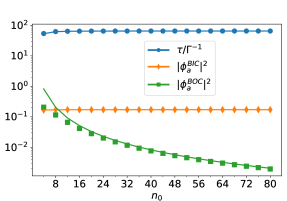
Figure 3: A plot showing how the emitter probabilities for the BICs, given by $|\phi_{a}^{(\text{BIC})}|^{2}$ and the BOCs, given by $|\phi_{a}^{(\text{BOC})}|^{2}$ scale as the number of sites $n_{0}$ between each coupling point increases. On this figure we show the values computed numerically (scatter plot) as well as the values computed from our asymptotic expansions (continuous lines) as $n_{0}\to\infty$ for the case where there are $M=3$ coupling points between the giant atom the the 1D lattice chain. On the same figure we also plot how $\tau/\Gamma^{-1}$ scales with $n_{0}$. As can be seen, as $\tau/\Gamma^{-1}$ increases and saturates at a value given by Eq. (24), $|\phi_{a}^{(\text{BIC})}|^{2}$ also increases and saturates at a value given by Eq. (22). On the other hand, $|\phi_{a}^{(\text{BOC})}|^{2}$ decreases monotonically with increasing $n_{0}$. We see that clearly, as the amount of non-Markovianity $\tau/\Gamma^{-1}$ in our system increases, we get better oscillating bound states.

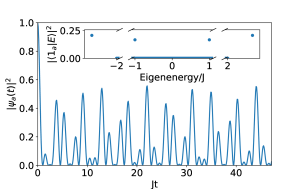
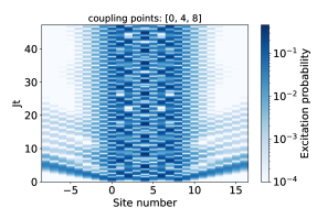
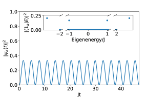
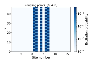
 (a)  (b)  (c)  (d)

Figure 4: Similar to Fig. 2, in (a) and (b) we consider the case of giant atom decay into the 1D lattice chain but with $M=3$ coupling points and $n_{0}=4$ sites between each coupling point. In (c) and (d), we also consider the case where we have $M=3$ coupling points and $n_{0}=4$ sites but with the giant atom lattice site initially in the vacuum state and the 1D lattice chain initialized in the state $|p\rangle$ according to Eq. (III.2). Remarkably, using Eq. (20), the required giant atom coupling strength is $\rho_{0}/J=1$. Due to the presence of the two BOCs with large emitter probabilities, for the case of the giant atom decay in (a) and (b), we see that the oscillation of the giant atom excitation probability in (a) is highly non-sinusoidal. Moreover, in (b), we see that there is a leakage of photon excitation probability beyond the coupling points due to the presence of the BOC, which is non-ideal. In (c) and (d), we see that because we are starting in the BIC subspace, the contributions due to the BOCs are totally eliminated. We see perfectly sinusoidal oscillations of the giant atom excitation probability in (c), and we also see that the photon excitation probability is strictly confined to within the coupling points of the giant atom to the 1D lattice.

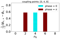
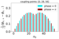
 (a)  (b)  (c)

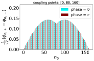
Figure 5: Here we show the amplitudes and the phases of the photonic excitation required to initialize the 1D lattice chain in the state $|p\rangle$ given by Eq. (III.2) for the case of $M=3$ coupling points between the giant atom and the 1D lattice chain. In (a),(b),(c), we plot the cases where we have $n_{0}=4$, $n_{0}=28$ and $n_{0}=80$ respectively. Sites with a phase of $0$ are indicated by a blue (lighter) color with a striped line within, whereas sites with a phase of $\pi$ are indicated by the a solid red (darker) color.

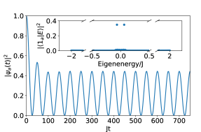
 (a)  (b)

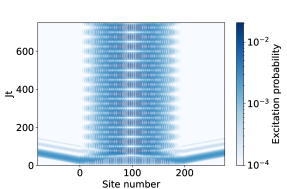
Figure 6: The analog of Fig. 2 except that we have $M=50$ coupling points between the giant atom and the 1D photonic lattice for $n_{0}=4$. As can be seen from the inset of (a), the emitter probabilities from the BOC are heaviliy suppressed as per Eq. (26) which leads to perfectly sinusoidal oscillations of the excitation probability of the giant atom lattice site. We also see in (b) that the negligible BOC emitter probability leads to an absence of loss of photonic excitation probability into the 1D lattice chain. By comparing (a) in this figure to Fig. 2, we see that a larger value of $M$ leads to larger amplitude oscillations in the excitation probability of the giant atom lattice site even for a comparatively small value of $n_{0}$, as per Eq. (21).

V Experimental implementation

The Hamiltonian in Eq. (1) can be simulated on a variety of platforms, such as coupled cavity arrays Hartmann et al. (2008); Majumdar et al. (2012) and photonic waveguide arrays Christodoulides et al. (2003); Longhi (2009); Szameit and Nolte (2010); Aspuru-Guzik and Walther (2012); Garanovich et al. (2012). In the case of a photonic waveguide array, we would have one photonic waveguide, which we call the giant atom waveguide, coupled to $M$ different photonic waveguides that are already coupled to each other to form a linear chain of $N$ waveguides, where the coupling is due to the evanescent field produced by the photon propagating within the waveguide. As the photon propagates in the waveguide, we have the relation $z=ct$, where $c$ is the group velocity of the photon in the waveguide and $z$ is the distance along the waveguide that the photon has propagated for.

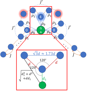
Figure 7: Possible experimental setup to see oscillating BICs. Here, we have $M=3$ and $n_{0}=4$. The giant atom waveguide is in green, with the letters “GA” inside whereas the waveguides in the waveguide chain are in blue. The coupling strength $\rho_{0}$ can be found from Eq. (20). Here, $\rho_{1}$ is the coupling between the giant atom and the next-nearest neighbor sites and $J^{\prime}$ is the hopping strength between the sites that are $\pm 1$ from the coupling point. In this set-up, we start with the giant atom in the vacuum state and instead initialize the rest of the waveguide chain in the state $|p\rangle$ according to Eq. (III.2). This means that as per Fig. 5 for the case where $n_{0}=4$, we need to send in a photon with equal probability amplitude in waveguides $2$, $4$, $6$ which we have highlighted. The red glow (site 2,6) indicates a phase of $\pi$ for the photon, whereas a waveguide with blue glow (site 4) indicate a phase of $0$. For the array of photonic waveguides, the coupling strength between each waveguide decays exponentially with the distance between the waveguides Jiao et al. (2021), hence by choosing the distances $d,d_{1}$ in the experimental setup appropriately as per the inset, we can obtain $\rho_{1}\ll\rho_{0}$ and $J^{\prime}\ll J$ which allow us to neglect the next-nearest neighbor interactions.

Following our formalism above, the nearest-neighbour coupling of the photonic waveguides in the linear chain with coupling strength $J$ gives us the tight binding Hamiltonian $H_{\text{wg}}$, whereas the coupling between the giant atom waveguide and the linear chain of waveguides at $M$ different points, each spaced $n_{0}$ apart, with coupling strength $\rho_{0}$ gives us the interaction Hamiltonian $H_{\text{int}}$. Taking the constraints of current experimental capabilities in mind, we propose an experimental setup for the case where $M=3$ and $n_{0}=4$ using the BIC subspace initialization in Fig. 7. For this photonic waveguide array system, the BIC initialization according to Fig. 7 can be achieved deterministically with a spatial light modulator that modulates a single photon source Tentrup et al. (2017). Alternatively, one can also prepare the oscillating BIC probabilistically by initializing an excitation only in the giant atom waveguide and perform photodetection on the sites outside of the giant atom coupling points, and postselect on the no-detection events.

In Fig. 7 we have also denoted the next-nearest neighbor coupling between the giant atom waveguide and the sites $0\pm 1$, $n_{0}\pm 1$ and $2n_{0}\pm 1$ with $\rho_{1}$, and also the next-nearest neighbor hopping between the lattice sites $0\pm 1$, $n_{0}\pm 1$ and $2n_{0}\pm 1$ with $J^{\prime}$. In general, the presence of $J^{\prime}$ and $\rho_{1}$ are unwanted imperfections, yet we note that by choosing the geometry and the distances accordingly as per the inset in Fig. 7, we can minimize the contributions from $\rho_{1}$ as well as $J^{\prime}$. To do so, we first use Eq. (19) to calculate the emitter energies for $n_{0}=4$, which would give us the oscillation period $T=\pi$ for the oscillating BIC. This means that to see an appreciable number of oscillations, we could simulate up to $Jz=5T\approx 15$. Now, suppose that experimentally, we can only have photonic waveguides with length $z_{\text{max}}$. This means that we require $J=5T/z_{\text{max}}$. Henceforth, we shall assume $z_{\text{max}}=100$ mm which has been done experimentally before Tang et al. (2022). From Eq. (20), we obtain $\rho_{0}/J=1$ which tells us to set $\rho_{0}=J$. It is known that the evanescent coupling strength between waveguides decay exponentially with the distance between them Jiao et al. (2021). Using the experimental values obtained in Jiao et al. (2021) for the aforementioned exponential relationship between coupling strength and distance, together with the geometry of the proposed setup in the inset of Fig. 7, we obtain $\rho_{0}=J=0.15\,\text{mm}^{-1}$, $\rho_{1}=0.0286\rho_{0}$ and $J^{\prime}=0.0286J$ which is nearly negligible. Thus, our proposed oscillating BICs are experimentally feasible using state-of-the-art photonic waveguide arrays.

Simulation results for $M=3$ and $n_{0}=4$ when $\rho_{1}=0$ and $J^{\prime}=0$ can be found in Fig. 4. The corresponding results when $\rho_{1}=0.0286\rho_{0}$ and $J^{\prime}=0.0286J$ can be found in Fig. 8.

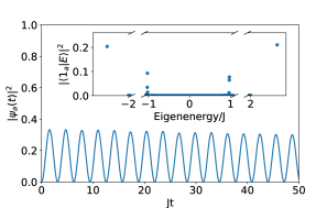
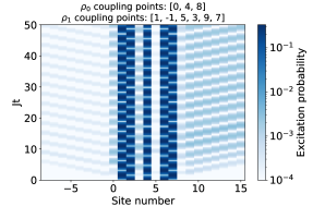
 (a)  (b)

Figure 8: Simulation results for the proposed experimental implementation with the setup in Fig. 7. Here, we initialize the waveguide array in the state $|p\rangle$ and with the giant atom lattice site in the vacuum state. Also, with reference to Fig. 7, we consider the case where we have $\rho_{1}=0.0286\rho_{0}$ and $J^{\prime}=0.0286J$ to show the impact of these experimental imperfections on our simulation. The corresponding ideal case for which $\rho_{1}=J^{\prime}=0$ can be found in (c) and (d) of Fig. 4. By comparing the ideal case with (a) and (b) in this figure, we see that the presence of experimental imperfections leads to a leakage of photon excitation probability beyond the coupling points of the giant atom, yet the effect is nearly negligible up to $Jz=15$, which is a large enough value of $Jz$ to see an appreciable number of oscillations.

VI Conclusion

In this paper, we study the phenomenon of oscillating BIC in a discrete 1D photonic lattice using a single emitter coupled to multiple lattice sites, which can be considered as the discrete analog of a giant atom coupled to a continuous waveguide. The key difference between our work and the oscillating BICs found in continuous waveguide systems Guo et al. (2020) is the presence of a finite energy band, which contributes band-edge effects to the giant atom dynamics. This gives us new conditions for the existence of oscillating BICs which lead to persistent oscillations of energy between the coupling points of the giant atom to the 1D lattice. The presence of bound states outside the continuum (BOC) hinders the trapping of excitation between the giant atom coupling points and is detrimental to the sinusoidal oscillations in the giant atom probability. Crucially, we find that these unwanted BOCs can be suppressed drastically by increasing either the number of coupling points $M$ or the number of lattice sites $n_{0}$ between each coupling point, with the BOC contribution scaling as $1/M^{2}$ and $1/n_{0}^{2}$. With this, we can summarize our key results for the conditions to produce optimal oscillating BICs to be: (1) $n_{0}=4l,l\in\mathbb{Z}^{+}$ sites between each coupling point, (2) Large $n_{0}$ and (3) Large M. In practice however, we find that a moderate $M$ and $n_{0}$ suffice to achieve good oscillating BICs with significant giant atom probability. Alternatively, by initializing the lattice sites in the BIC subspace which we have calculated, the BOC contributes can be completely eliminated, resulting in perfect oscillating BICs even for small $M$ and $n_{0}$. We stress that the oscillating BIC in our system is inherently a non-Markovian phenomenon due to the significant propagation time between the giant atom coupling points compared to the relaxation timescale of the giant atom. Moreover, we show that as the non-Markovianity in our system increases, the oscillation amplitude of the BICs increases, improving the storage of quantum information within the coupling points. To illustrate the feasibility of our theoretical model, we propose an experimental implementation of our system on photonic waveguide arrays and show that our oscillating BICs can be practically achieved even with current experimental limitations.

Our work provides a firm theoretical basis for oscillating BICs in discrete systems. In particular, oscillating BICs in discrete systems offer new possibilities that cannot be replicated in continuous systems, such as the ability to initialize the system in the BIC subspace by simply controlling the amplitude and phase of the excitation at particular lattice sites. This allows us to achieve long-time storage of quantum information within the confines of the giant atom coupling points, limited only by the intrinsic coherence time of the photonic lattice. Our setup can also be regarded as an effective cavity, serving as a physical implementation of non-Markovian cavity-QED setups Crowder et al. (2020); Arranz Regidor and Hughes (2021); Guimond et al. (2016); Černotík et al. (2019); Du et al. (2021). While we have considered the tight-binding dispersion relation in this work, the phenomenon of oscillating BICs can be generally observed in discrete systems with other dispersion relations, which can be considered for future work. Another promising direction is to study the oscillating BIC phenomenon in higher-dimensional lattices González-Tudela et al. (2019) or in synthetic dimensions Du et al. (2022); Xiao et al. (2022).

Appendix A Writing Eq. (1) in $k$-space

From Eq. (3), we can express $H_{\text{wg}}$ as

$$H_{\text{wg}}= J\sum_{n}b_{n}^{\dagger}b_{n+1}+\text{H.c}$$

$$= \frac{J}{2\pi}\iint dk\,dk^{\prime}\sum_{n}e^{i(k^{\prime}-k)n}e^{ik^{\prime}}c^{\dagger}(k)c(k^{\prime})+\frac{J}{2\pi}\iint dk\,dk^{\prime}\sum_{n}e^{-i(k^{\prime}-k)n}e^{-ik^{\prime}}c^{\dagger}(k^{\prime})c(k)$$

$$= \frac{J}{2\pi}\iint dk\,dk^{\prime}\sum_{n}e^{i(k^{\prime}-k)n}e^{ik^{\prime}}c^{\dagger}(k)c(k^{\prime})+\frac{J}{2\pi}\iint dk^{\prime}\,dk\sum_{n}e^{-i(k-k^{\prime})n}e^{-ik}c^{\dagger}(k)c(k^{\prime})$$

$$= J\iint dk\,dk^{\prime}\left(\frac{1}{2\pi}\sum_{n}e^{i(k^{\prime}-k)n}\right)\left(e^{ik^{\prime}}+e^{-ik}\right)c^{\dagger}(k)c(k^{\prime})$$

$$= J\iint dk\,dk^{\prime}\delta(k^{\prime}-k)\left(e^{ik^{\prime}}+e^{-ik}\right)c^{\dagger}(k)c(k^{\prime})$$

$$= J\int dk\,\left(e^{ik}+e^{-ik}\right)c^{\dagger}(k)c(k)$$

$$= \int dk\,2J\cos(k)c^{\dagger}(k)c(k)$$

$$= \int dk\,\omega(k)c^{\dagger}(k)c(k),$$ (31)

where we have defined $\omega(k)\equiv 2J\cos(k)$. Here, we have used the fact that for $(k^{\prime}-k)\in[0,2\pi)$, $\frac{1}{2\pi}\sum_{n}e^{i(k^{\prime}-k)n}=\delta(k^{\prime}-k)$. Similarly, we can also express $H_{\text{int}}$ as

$$H_{\text{int}} =\sum_{j=1}^{k}\rho_{j}(a^{\dagger}b_{n_{j}}+\text{H.c})$$

$$=\sum_{j=1}^{k}\rho_{j}\left\{a^{\dagger}\left(\frac{1}{\sqrt{2\pi}}\int_{-\pi}^{\pi}dk\,e^{ikn_{j}}c(k)\right)+\text{H.c}\right\}$$

$$=\int_{-\pi}^{\pi}dk\,\left\{\left(\frac{1}{\sqrt{2\pi}}\sum_{j=1}^{k}\rho_{j}e^{ikn_{j}}\right)a^{\dagger}c(k)+\text{H.c}\right\}$$

$$\equiv\int_{-\pi}^{\pi}dk\,\left\{G(k)a^{\dagger}c(k)+\text{H.c}\right\},$$ (32)

where we have defined $G(k)=\left(\frac{1}{\sqrt{2\pi}}\sum_{j=1}^{K}\rho_{j}e^{ikn_{j}}\right)$.

Appendix B Derivation of conditions for BIC

First, to derive Eq. (6) and the condition for the BIC to have a finite norm , we shall first write our energy eigenstate in the one-excitation subspace as

$$|E\rangle=\phi_{a}|1_{a}\rangle+\int dk\,e(k)|1_{k}\rangle$$ (33)

where $\phi_{a}=\langle 1_{a}|E\rangle$ and $e(k)=\langle 1_{k}|E\rangle$. Thereafter, we consider the energy eigenvalue equation $H|E\rangle=\Omega|E\rangle$. To evaluate $H|E\rangle$, we use the commutation relations $[a,a^{\dagger}]=1$ and $[c(k),c^{\dagger}(k^{\prime})]=\delta(k-k^{\prime})$, and finally we arrive at

$$H|E\rangle=\left(\omega_{a}\phi_{a}+\int dk\,G(k)e(k)\right)|1_{a}\rangle+\int dk\,\left(\omega(k)e(k)+G^{*}(k)\phi_{a}\right)|1_{k}\rangle.$$ (34)

Comparing the above equation with $\Omega|E\rangle=\Omega(\phi_{a}|1_{a}\rangle+\int dk\,e(k)|1_{k}\rangle)$, we arrive at two simultaneous equations

$$\Omega\phi_{a} =\omega_{a}\phi_{a}+\int dk\,G(k)e(k)$$ (35a)

$$\Omega e(k) =\omega(k)e(k)+G^{*}(k)\phi_{a}$$ (35b)

which we can then solve to obtain Eq. (6). Next, we note that in the one-excitation subspace, we have

$$\langle E|E\rangle =|\phi_{a}|^{2}+\int dk\,|e(k)|^{2}$$

$$=|\phi_{a}|^{2}\left(1+\int dk\,\frac{|G(k)|^{2}}{(\Omega-\omega(k))^{2}}\right)$$

$$=|\phi_{a}|^{2}\left(1+\int d\omega\,\frac{\rho(\omega)|G(k(\omega))|^{2}}{(\Omega-\omega)^{2}}\right)$$ (36)

where in the second line, we used Eq. (35b) and in the third line, we used $\rho(\omega)\equiv\frac{\partial k}{\partial\omega}$. Hence we see that the requirement that $|E\rangle$ has a finite norm corresponds to $\rho(\omega)|G(k(\omega))|^{2}$ vanishing at least as fast as $\sim(\Omega-\omega)^{2}$ as $\omega\to\Omega$.

Next, to derive Eq. (8), we note that

$$\Sigma(s=-i\Omega\pm 0^{+}) =\int_{-\pi}^{\pi}dk\frac{|G(k)|^{2}}{\Omega-\omega(k)}$$

$$=\int_{-2J}^{2J}d\omega\frac{\rho(\omega)|G(k(\omega))|^{2}}{\Omega-\omega}$$

$$=\lim_{\epsilon\to 0}\left(\int_{-2J}^{\Omega-\epsilon}d\omega\,\frac{\rho(\omega)|G(k(\omega))|^{2}}{\Omega-\omega}+\int_{\Omega+\epsilon}^{2J}d\omega\,\frac{\rho(\omega)|G(k(\omega))|^{2}}{\Omega-\omega}\right)+\int_{C}d\omega\,\frac{\rho(\omega)|G(k(\omega))|^{2}}{\Omega-\omega}$$

$$=\mathcal{P}\left(\int_{-2J}^{2J}d\omega\frac{\rho(\omega)|G(k(\omega))|^{2}}{\Omega-\omega}\right)\mp i\pi\rho(\Omega)|G(k(\Omega))|^{2}$$ (37)

where in the second last line, we note that the contour $C$ is a semi-circular contour either in the top half or bottom half of the complex plane, depending on the sign of $\pm 0^{+}$, and in the last line we used the residue theorem for the special case of a semi-circular contour. $\mathcal{P}()$ here denotes the Cauchy Principal value of the integral enclosed in the parentheses. Taking the real part of the last line, Eq. (8) follows immediately. We note here that if $\Omega$ also fulfils Eq. (4), then the second term vanishes, which gives us

$$\Sigma(s=-i\Omega\pm 0^{+})=\text{Re}[\Sigma(s=-i\Omega\pm 0^{+})].$$ (38)

Appendix C Decay dynamics

Here, we derive Eq. (9). By writing down the Schrodinger equation $H|\psi(t)\rangle=i\frac{\partial}{\partial t}|\psi(t)\rangle$ in the one-excitation subspace as per Eq. (5), we arrive at two coupled equations

$$i\frac{\partial\psi_{a}(t)}{\partial t} =\omega_{a}\psi_{a}(t)+\int_{-\pi}^{\pi}G(k)\psi(k,t)dk$$ (39a)

$$i\frac{\partial\psi(k,t)}{\partial t} =\omega(k)\psi(k,t)+G^{*}(k)\psi_{a}(t).$$ (39b)

To solve the two above equations for $\psi_{a}(t)$, we follow the standard procedure of first integrating the “bath” equation, which is Eq. (39b) in our case, to get

$$\psi(k,t)=-iG^{*}(k)e^{-i\omega(k)t}\int_{0}^{t}dt^{\prime}e^{i\omega(k)t^{\prime}}\psi_{a}(t^{\prime})+e^{-i\omega(k)t}\psi(k,0).$$ (40)

Then, we substitute the above equation into Eq. (39a) to get

$$\frac{\partial\psi_{a}(t)}{\partial t}=-i\omega_{a}\psi_{a}(t)-\int_{-\pi}^{\pi}dk\,|G(k)|^{2}e^{-i\omega(k)t}\int_{0}^{t}dt^{\prime}\,e^{i\omega(k)t^{\prime}}\psi_{a}(t^{\prime})-iA(t)$$ (41)

where $A(t)\equiv\int_{-\pi}^{\pi}dk\,G(k)e^{-i\omega(k)t}\psi(k,0)$. Next, we take the Laplace transform on both sides of the above equation by defining $\tilde{\psi}_{a}(s)=\int_{0}^{\infty}dt\,e^{-st}\psi_{a}(t)$. By also using the fact that $\int_{0}^{\infty}dt\,e^{-st}\frac{\partial\psi_{a}(t)}{\partial t}=s\tilde{\psi}_{a}(s)-\psi_{a}(0)$, and defining $\tilde{A}(s)$ as the Laplace transfrom of $A(t)$, we arrive at

$$s\tilde{\psi}_{a}(s)-\psi_{a}(0)=-i\omega_{a}\tilde{\psi}_{a}(s)-i\tilde{A}(s)-\int_{-\pi}^{\pi}dk\,|G(k)|^{2}\int_{0}^{\infty}dt\,e^{-(s+i\omega(k))t}F(t)$$ (42)

where $F(t)\equiv\int_{0}^{t}dt^{\prime}e^{i\omega(k)t^{\prime}}\psi_{a}(t^{\prime})$. Realising that $\frac{d}{dt}F(t)=e^{i\omega(k)t}\psi_{a}(t)$, we perform integration by parts on $\int_{0}^{\infty}dt\,e^{-(s+i\omega(k))t}F(t)$ and after some algebra finally arrive at

$$\left(s+i\omega_{a}+i\Sigma(s)\right)\tilde{\psi}_{a}(s)=-i\tilde{A}(s)+\psi_{a}(0)$$ (43)

where $\Sigma(s)$ as per defined in Eq. (7). By inserting into the above equation the initial conditions corresponding to the case of giant atom decay, $\psi_{a}(0)=1$ and $\psi(k,0)=0$ for all $k$, we finally arrive at

$$\tilde{\psi}_{a}(s)=\frac{1}{s+i\omega_{a}+i\Sigma(s)}$$ (44)

which we can invert via the Bromwich integral to give us $\psi_{a}(t)$ in the following manner,

$$\psi_{a}(t) =\frac{1}{2\pi i}\int_{\lambda-i\infty}^{\lambda+i\infty}\frac{e^{st}}{s+i\omega_{a}+i\Sigma(s)}$$

$$=\sum_{\text{All residues}}\frac{e^{st}}{s+i\omega_{a}+i\Sigma(s)}$$

where to go from the first line to the second line, we pick $\lambda$ sufficiently large so that all the poles of the integrand lie on the left of the line $\lambda+it$, $t\in(-\infty,\infty)$. The second line is Eq. (9) in the main text. We note that in going from the first line to the second line, we have ignored the contributions from the integration over any paths induced by possible branch cuts. This is because we will mainly use the above equation to study the behavior of BICs, which are poles on the imaginary axis and hence lead to long-term, non-decaying behavior of $\psi_{a}(t)$. The integration over any paths induced by possible branch cuts leads to transient decay behavior which we are not interested in.

Appendix D Detailed calculations for section III in the main text

D.1 Derivation of Eq. (16)

First of all, we note the important integral result

$$I_{n}(s) =\int_{-\pi}^{\pi}dk\,\frac{e^{ikn}}{is-\cos(k)}$$

$$=\frac{-2\pi i}{\sqrt{s^{2}+1}}\left(is\mp i\sqrt{s^{2}+1}\right)^{|n|}$$ (45)

where we have the minus sign when $\text{Re}(s)>0$ and the positive sign when $\text{Re}(s)<0$. The result can be derived by making the subtitution $z=e^{ik}$ and thereafter computing the resultant complex integral

$$I_{n}(s) =\oint_{C}dz\,\frac{z^{n}}{is-(1/2)(z+z^{-1})}\frac{1}{iz}$$

$$=2i\oint_{C}dz\,\frac{z^{n}}{z^{2}-2isz+1}$$

$$=2i\oint_{C}dz\,\frac{z^{n}}{(z-z_{1})(z-z_{2})}$$ (46)

where the contour $C$ is the unit circle in the complex plane and $z_{1}=i(s+\sqrt{s^{2}+1})$, $z_{2}=i(s-\sqrt{s^{2}+1})$. The above integral can then be easily evaluated by the Cauchy Residue Theorem. Now, we can show that $\text{Re}(s)>0$ implies that $|z_{1}|>1$, $|z_{2}|<1$ which means that $z_{2}$ is a simple pole in $C$. On the other hand, $\text{Re}(s)<0$ implies that $|z_{1}|<1$, $|z_{2}|>1$ which means that $z_{1}$ is a simple pole in $C$. Moreover, if $n<0$ then we also have a $n$th order pole at z=0 in $C$. Putting all of these together with the fact that $z_{1}z_{2}=1$ which means that $z_{1}^{-|n|}=z_{2}^{|n|}$, we can arrive at Eq. (D.1) after some algebra.

Thereafter, using the above result we can easily derive the following integral, with $n$ being a non-negative integer

$$\int_{-\pi}^{\pi}dk\frac{\cos(nk)}{is-2J\cos(k)}=\frac{-2\pi i}{\sqrt{s^{2}+4J^{2}}}\left(\frac{is\mp i\sqrt{s^{2}+4J^{2}}}{2J}\right)^{n}$$ (47)

where again we have the minus sign when $\text{Re}(s)>0$ and the positive sign when $\text{Re}(s)<0$. Next, we can derive

$$|G(k)|^{2} =\frac{\rho^{2}}{2\pi}\sum_{j=0}^{M-1}\sum_{l=0}^{M-1}e^{ikn_{0}(j-l)}$$

$$=\frac{\rho^{2}}{2\pi}\left(M+2\sum_{r=1}^{M-1}(M-r)\cos(kn_{0}r)\right)$$ (48)

where in going from the first line to the next, we realise that there are $M$ terms of $e^{ik(0)n_{0}}$, $(M-1)$ terms of $e^{ik(1)n_{0}}$ and its complex conjugate, $(M-2)$ terms of $e^{ik(2)n_{0}}$ and its complex conjugate, and so on, until at last we have $1$ term of $e^{ik(M-1)n_{0}}$ and its complex conjugate. With the form of $|G(k)|^{2}$ above and Eq. (47), we can get Eq. (16) from Eq. (7).

D.2 Derivation of oscillating BIC conditions

Since we are working with $\omega_{a}=0$, we want to look for two BICs as near the band centre as possible with energies $\pm\Omega_{\text{BIC}}$, where $\Omega_{\text{BIC}}$ is a positive value to be determined. Hence, we want to minimise the quantity

$$\left|\frac{\Omega}{2J}\right|=\cos\left(\frac{2\pi}{n_{0}}\left(m\pm\frac{1}{M}\right)\right)$$ (49)

over all integer values of $m$. Note that in the above expression, we have already substituted Eq. (15) into the dispersion relation $\omega(k)=2J\cos(k)$. One way to perform this minimization is to first solve $m$ in the equation $|\Omega/2J|=0$ and then rounding the value of $m$ to the closest integer. When we solve $|\Omega/2J|=0$, we obtain two cases

$$\frac{2\pi}{n_{0}}\left(m\pm\frac{1}{m}\right)=\frac{\pi}{2}\implies m=\frac{n_{0}}{4}\mp\frac{1}{m}$$ (50a)

$$\frac{2\pi}{n_{0}}\left(m\pm\frac{1}{m}\right)=\frac{3\pi}{2}\implies m=\frac{3n_{0}}{4}\mp\frac{1}{m}.$$ (50b)

At this juncture, before we round the value of $m$ obtained above to the closest integer, we note that there are two cases we need to consider: either $n_{0}=2(2l)$ or $n_{0}=2(2l+1)$ where $l\in\mathbb{Z}$. In the former case where $n_{0}=4l$, the closest integer value of $m$ would be $m=n_{0}/4$ or $m=3n_{0}/4$, which would give us the BIC frequencies in Eq. (19) when we substitute those values of $m$ into Eq. (49). Thereafter, we can obtain $\rho_{0}$ by substituting those frequencies into Eq. (18) to obtain Eq. (20).

In the latter case where $n_{0}=4l+2$, the closest integer values of $m$ would be $m=n_{0}/4\pm 1/2$ or $m=3n_{0}/4\pm 1/2$, corresponding to two possible BIC frequencies,

$$\Omega_{\text{BIC}}=\sin\left(\frac{\pi}{n_{0}}\left(1\pm\frac{2}{M}\right)\right).$$

However, when we substitute $\Omega_{\text{BIC}}=\sin((\pi/n_{0})(1-2/M))$ into Eq. (18), for the case of $\omega_{a}=0$, we end up with $\rho_{0}^{2}<0$, which means that we are only left with $\Omega_{\text{BIC}}=\sin((\pi/n_{0})(1+2/M))$ for the $n_{0}=4l+2$ case. However, since this is further from the band center as compared to the $n_{0}=4l$ case, the resultant bound states would have lower emitter probability. Hence, we can conclude that $n_{0}=4l$ would give optimal oscillating BICs.

As an example, for the case where $M=3$ and $n_{0}=4l+2,n_{0}>2$, we have the BIC frequency $|\Omega|=2J\sin\left(\frac{5\pi}{3n_{0}}\right)$ which gives us

$$\rho_{0}^{2}=\frac{2J^{2}}{\sqrt{3}}\sin\left(\frac{10\pi}{3n_{0}}\right)$$ (51)

Using Eq. (12), we find that the emitter probability

$$|\phi_{a}^{\text{BIC}}|^{2}\to\frac{9}{9+20\sqrt{3}\pi}\approx 0.0764$$ (52)

as $n_{0}\to\infty$, which is considerably smaller than the optimal value $\approx 0.171$ when $n_{0}$ is an integer multiple of $4$ for $M=3$.

D.3 Derivation of Eq. (25) and Eq. (26)

To derive Eq. (25), the method is to solve Eq. (16) using both Eq. (17) and Eq. (8) for the case where $\omega_{a}=0$ and $|\Omega|>2J$. The $|\Omega|>2J$ condition is because we are trying to solve for $\Omega$ outside the energy band. We note that there are two cases for us to consider, namely $\text{Re}(s)>0$, corresponding to $s=-i\Omega+0^{+}$ and $\text{Re}(s)<0$, corresponding to $s=-i\Omega-0^{+}$. As we will see, the $\text{Re}(s)>0$ case gives us the BOC energy for $\Omega<-2J$, and the $\text{Re}(s)<0$ case gives use the BOC energy for $\Omega>2J$. First, we consider the $\text{Re}(s)>0$ case. In this case, we have the equation

$$\left(\frac{\Omega}{2J}\right)^{2}=-\frac{1}{4}\left(\frac{\rho_{0}}{J}\right)^{2}\frac{1}{\sqrt{\left(\frac{\Omega}{2J}\right)^{2}-1}}\left(M+2\sum_{r=1}^{M-1}(M-r)\left(\frac{\Omega}{2J}+\sqrt{\left(\frac{\Omega}{2J}\right)^{2}-1}\right)^{n_{0}r}\right)$$ (53)

where we have used $\sqrt{4J^{2}-\Omega^{2}}=i\sqrt{\Omega^{2}-4J^{2}}$, since $|\Omega|>2J$. Now, we substitute $\Omega^{\prime}=\Omega/2J$ as well as Eq. (20) for $\rho_{0}/J$ to get

$$\Omega^{\prime}\sqrt{{\Omega^{\prime}}^{2}-1}=-\frac{1}{4}\frac{2}{M}\tan\left(\frac{\pi}{M}\right)\sin\left(\frac{4\pi}{Mn_{0}}\right)\left(M+2\sum_{r=1}^{M-1}(M-r)\left(\Omega^{\prime}+\sqrt{{\Omega^{\prime}}^{2}-1}\right)^{n_{0}r}\right)$$ (54)

In the $n_{0}\to\infty$ limit, for the above equation to have a solution, we must have $\Omega^{\prime}+\sqrt{{\Omega^{\prime}}^{2}-1}<1$, which means $\Omega<-2J$. Hence, taking the $n_{0}\to\infty$ limit, we have

$$\Omega^{\prime}\sqrt{{\Omega^{\prime}}^{2}-1}=-\frac{2}{M}\tan\left(\frac{\pi}{M}\right)\left(\frac{\pi}{Mn_{0}}\right)M$$ (55)

Solving for $\Omega^{\prime}$ in the above equation subject to the condition that $\Omega<-2J$, we have

$$\Omega^{\prime} =-\sqrt{\frac{1}{2}\sqrt{\frac{16\pi^{2}\tan^{2}\left(\frac{\pi}{M}\right)}{M^{2}\text{n0}^{2}}+1}+\frac{1}{2}}$$

$$\approx-1-\frac{2\pi^{2}\tan\left(\frac{\pi}{M}\right)^{2}}{M^{2}n_{0}^{2}}.$$ (56)

The last line in the above equation is Eq. (25) for the case where $\Omega<-2J$. The derivation for the $\Omega>2J$ case can be done by choosing $\text{Re}(s)<0$ and following the same steps above to arrive at

$$\Omega^{\prime} =\sqrt{\frac{1}{2}\sqrt{\frac{16\pi^{2}\tan^{2}\left(\frac{\pi}{M}\right)}{M^{2}\text{n0}^{2}}+1}+\frac{1}{2}}$$

$$\approx 1+\frac{2\pi^{2}\tan\left(\frac{\pi}{M}\right)^{2}}{M^{2}n_{0}^{2}}$$ (57)

where the last line in the above equation is Eq. (25) for the case where $\Omega>2J$. To derive Eq. (26), the method is to use Eq. (12) together with Eq. (16) and Eq. (8). We will also use Eq. (25) derived above, and also Eq. (20) for $\rho_{0}/J$. Thereafter, doing an asymptotic expansion about $\frac{1}{n_{0}}\to 0$ and keeping the lowest order, we obtain Eq. (26).

D.4 Derivation of Eq. (28)

Firstly, we write our BICs $|\pm\rangle$ as

$$|\pm\rangle =\phi_{a}^{(\pm)}|1_{a}\rangle+\int_{-\pi}^{\pi}dk\,e(k)^{\pm}|1_{k}\rangle$$

$$=\phi_{a}^{(\pm)}|1_{a}\rangle+\phi_{a}^{(\pm)}\int_{-\pi}^{\pi}dk\,\frac{G^{*}(k)}{\Omega_{\pm}-2J\cos(k)}|1_{k}\rangle$$ (58)

where $\phi_{a}^{(\pm)}=\langle 1_{a}|\pm\rangle$ and $e(k)^{\pm}=\langle 1_{k}|\pm\rangle$, and $\Omega_{\pm}$ is the energy of the $|\pm\rangle$ state respectively. In going from the first line to the second line, we used Eq. (35). In the second line above, we see that we can clearly factor out a global phase corresponding to the phase of $\langle 1_{a}|\pm\rangle$. Hence, without loss of generality, we can write $\phi_{a}\equiv\phi_{a}^{(\pm)}=\langle 1_{a}|\pm\rangle$. Then, we have

$$|\pm\rangle =\phi_{a}|1_{a}\rangle+\phi_{a}\int_{-\pi}^{\pi}dk\,\frac{G^{*}(k)}{\Omega_{\pm}-2J\cos(k)}|1_{k}\rangle$$

$$=\phi_{a}|1_{a}\rangle+\phi_{a}\int_{-\pi}^{\pi}dk\,\frac{G^{*}(k)}{\Omega_{\pm}-2J\cos(k)}c(k)^{\dagger}|0\rangle$$

$$=\phi_{a}|1_{a}\rangle+\phi_{a}\int_{-\pi}^{\pi}dk\,\frac{G^{*}(k)}{\Omega_{\pm}-2J\cos(k)}\sum_{n}e^{ikn}\frac{1}{\sqrt{2\pi}}b_{n}^{\dagger}|0\rangle$$

$$=\phi_{a}|1_{a}\rangle+\phi_{a}\int_{-\pi}^{\pi}dk\,\frac{(\rho_{0}/2\sqrt{\pi})\sum_{l=0}^{M-1}e^{-ikn_{l}}}{\Omega_{\pm}-2J\cos(k)}\sum_{n}e^{ikn}\frac{1}{\sqrt{2\pi}}b_{n}^{\dagger}|0\rangle$$

$$=\phi_{a}|1_{a}\rangle+\sum_{n}\underbrace{\frac{\rho_{0}\phi_{a}}{2\pi}\sum_{l=0}^{M-1}\int_{-\pi}^{\pi}dk\,\frac{e^{ik(n-n_{l})}}{\Omega_{\pm}-2J\cos(k)}}_{\equiv\phi_{n,\pm}}b_{n}^{\dagger}|0\rangle$$ (59)

Thereafter, to evaluate $\phi_{n,\pm}$, we note that

$$\phi_{n,\pm} =\frac{\rho_{0}\phi_{a}}{2\pi}\sum_{l=0}^{M-1}\int_{-\pi}^{\pi}dk\,\frac{e^{ik(n-n_{l})}}{\Omega_{\pm}-2J\cos(k)}$$

$$=\frac{\rho_{0}\phi_{a}}{2\pi}\sum_{l=0}^{M-1}I_{n-n_{l}}(s=-i\Omega_{\pm}+0^{+})$$ (60)

where $I_{n-n_{l}}(s)$ is given by Eq. (D.1).

Appendix E Proof that there is no oscillating BIC with $M=2$

For $n=2$, we have

$$|G(k)|^{2}=\frac{\rho_{0}^{2}}{\pi}\left(1+\cos(kn_{0})\right)$$ (61)

which gives us

$$\Sigma(s)=\frac{-2i\rho_{0}^{2}}{\sqrt{s^{2}+4J}}\left(1+\left(\frac{-i\sqrt{s^{2}+4J^{2}}+is}{2J}\right)^{n_{0}}\right).$$ (62)

Thus, we have

$$\Sigma(s=-i\Omega) =\frac{-2i\rho_{0}^{2}}{\sqrt{4J-\Omega^{2}}}\left(1+\left(\frac{-i\sqrt{4J^{2}-\Omega^{2}}+\Omega}{2J}\right)^{n_{0}}\right)$$

$$=\frac{-2i\rho_{0}^{2}}{\sqrt{4J-\Omega^{2}}}\left(1+\cos(n_{0}\theta)+i\sin(n_{0}\theta)\right)$$ (63)

where $\theta=\arctan\left(\frac{-\sqrt{4J^{2}-\Omega^{2}}}{\Omega}\right)$ and $-2J<\Omega<2J$. Using $\Delta(\Omega)=\text{Re}(\Sigma(s=-i\Omega+0^{+}))$, we have

$$\Omega-\omega_{a}=\frac{2\rho_{0}^{2}}{\sqrt{4J-\Omega^{2}}}\sin(n_{0}\theta)$$ (64)

Furthermore, enforcing $|G(k)|^{2}=0$ gives us

$$k=(2l+1)\frac{\pi}{n_{0}}$$ (65)

where $l$ is an integer. Hence, we have

$$\Omega=2J\cos\left(\frac{\pi}{n_{0}}(2l+1)\right)$$ (66)

which we can substitute into $\theta=\arctan\left(\frac{-\sqrt{4J^{2}-\Omega^{2}}}{\Omega}\right)$ to get

$$\theta=-\frac{\pi}{n_{0}}(2l+1)$$ (67)

Subtituting the above expression into Eq. (64), we have

$$\Omega=\omega_{a}.$$ (68)

Hence, when we have $K=2$ legs in our giant atom, there is only one BIC at the frequency $\Omega=\omega_{a}$, provided that

$$\omega_{a}=\Omega=2J\cos\left(\frac{\pi}{n_{0}}(2l+1)\right).$$ (69)

Otherwise, there is no BIC for $K=2$ legs. Moreover, since we only have one BIC, it is impossible to get an oscillating BIC, which requires at least two BICs at two different frequencies in the band.

Appendix F Comparison of the oscillating BIC conditions with continuous waveguide

For $M$ coupling points, and setting $\omega_{a}=0$, the oscillating BIC found for a continuous (linearized) waveguide in Ref. Guo et al. (2020) are formed from the superposition of two BICs with energies

$$\Omega_{c}=\pm\frac{1}{2}M\gamma\cot\left(\frac{n\pi}{M}\right),\quad n=1,2,\ldots,\left\lfloor M/2\right\rfloor$$ (70)

where $\gamma$ is the giant atom decay rate into the waveguide. In our case, $\gamma$ corresponds to $\rho_{0}^{2}/J$. From Eq. (19) and Eq. (20), we have, for our case,

$$\Omega_{\text{BIC}}=\pm 2J\sin\left(\frac{2\pi}{Mn_{0}}\right)=\pm 2\gamma\frac{J^{2}}{\rho_{0}^{2}}\sin\left(\frac{2\pi}{Mn_{0}}\right)=\pm\frac{1}{2}M\gamma\cot\left(\frac{\pi}{M}\right)\sec\left(\frac{2\pi}{Mn_{0}}\right)$$ (71)

which looks similar to the continuous-waveguide result for $n=1$. In fact, in the regime where $(Mn_{0})$ is large such that $\sec(2\pi/(Mn_{0}))\approx 1$, the oscillating BIC energies are approximately the same as $\Omega_{c}$.

References

- Ludlow et al. (2015) Andrew D. Ludlow, Martin M. Boyd, Jun Ye, E. Peik, and P. O. Schmidt, “Optical atomic clocks,” Rev. Mod. Phys. 87, 637–701 (2015).
- Bruzewicz et al. (2019) Colin D. Bruzewicz, John Chiaverini, Robert McConnell, and Jeremy M. Sage, “Trapped-ion quantum computing: Progress and challenges,” Applied Physics Reviews 6, 021314 (2019), https://doi.org/10.1063/1.5088164 .
- Duan and Monroe (2010) L.-M. Duan and C. Monroe, “Colloquium: Quantum networks with trapped ions,” Rev. Mod. Phys. 82, 1209–1224 (2010).
- Monroe et al. (2021) C. Monroe, W. C. Campbell, L.-M. Duan, Z.-X. Gong, A. V. Gorshkov, P. W. Hess, R. Islam, K. Kim, N. M. Linke, G. Pagano, P. Richerme, C. Senko, and N. Y. Yao, “Programmable quantum simulations of spin systems with trapped ions,” Rev. Mod. Phys. 93, 025001 (2021).
- Tannoudji et al. (1992) Claude Cohen Tannoudji, Gilbert Grynberg, and J Dupont-Roe, “Atom-photon interactions,” (1992).
- Liao et al. (2016) Zeyang Liao, Xiaodong Zeng, Hyunchul Nha, and M Suhail Zubairy, “Photon transport in a one-dimensional nanophotonic waveguide QED system,” Physica Scripta 91, 063004 (2016).
- Roy et al. (2017) Dibyendu Roy, C. M. Wilson, and Ofer Firstenberg, “Colloquium: Strongly interacting photons in one-dimensional continuum,” Rev. Mod. Phys. 89, 021001 (2017).
- Shen and Fan (2005a) Jung-Tsung Shen and Shanhui Fan, “Coherent single photon transport in a one-dimensional waveguide coupled with superconducting quantum bits,” Phys. Rev. Lett. 95, 213001 (2005a).
- Shen and Fan (2005b) J. T. Shen and Shanhui Fan, “Coherent photon transport from spontaneous emission in one-dimensional waveguides,” Opt. Lett. 30, 2001–2003 (2005b).
- Bajcsy et al. (2009) M. Bajcsy, S. Hofferberth, V. Balic, T. Peyronel, M. Hafezi, A. S. Zibrov, V. Vuletic, and M. D. Lukin, “Efficient all-optical switching using slow light within a hollow fiber,” Phys. Rev. Lett. 102, 203902 (2009).
- Akimov et al. (2007) Alexey Akimov, A Mukherjee, C Yu, D Chang, A. Zibrov, P Hemmer, H Park, and M Lukin, “Generation of single optical plasmons in metallic nanowires coupled to quantum dots,” Nature 450, 402–6 (2007).
- Huck and Andersen (2016) Alexander Huck and Ulrik L. Andersen, “Coupling single emitters to quantum plasmonic circuits,” Nanophotonics 5, 483–495 (2016).
- Arcari et al. (2014) M. Arcari, I. Söllner, A. Javadi, S. Lindskov Hansen, S. Mahmoodian, J. Liu, H. Thyrrestrup, E. H. Lee, J. D. Song, S. Stobbe, and P. Lodahl, “Near-unity coupling efficiency of a quantum emitter to a photonic crystal waveguide,” Phys. Rev. Lett. 113, 093603 (2014).
- Astafiev et al. (2010a) O. Astafiev, A. M. Zagoskin, A. A. Abdumalikov, Yu. A. Pashkin, T. Yamamoto, K. Inomata, Y. Nakamura, and J. S. Tsai, “Resonance fluorescence of a single artificial atom,” Science 327, 840–843 (2010a), https://www.science.org/doi/pdf/10.1126/science.1181918 .
- Astafiev et al. (2010b) O. V. Astafiev, A. A. Abdumalikov, A. M. Zagoskin, Yu. A. Pashkin, Y. Nakamura, and J. S. Tsai, “Ultimate on-chip quantum amplifier,” Phys. Rev. Lett. 104, 183603 (2010b).
- Abdumalikov et al. (2010) A. A. Abdumalikov, O. Astafiev, A. M. Zagoskin, Yu. A. Pashkin, Y. Nakamura, and J. S. Tsai, “Electromagnetically induced transparency on a single artificial atom,” Phys. Rev. Lett. 104, 193601 (2010).
- Chang et al. (2018) D. E. Chang, J. S. Douglas, A. González-Tudela, C.-L. Hung, and H. J. Kimble, “Colloquium: Quantum matter built from nanoscopic lattices of atoms and photons,” Rev. Mod. Phys. 90, 031002 (2018).
- Gu et al. (2017) Xiu Gu, Anton Frisk Kockum, Adam Miranowicz, Yu xi Liu, and Franco Nori, “Microwave photonics with superconducting quantum circuits,” Physics Reports 718-719, 1–102 (2017), microwave photonics with superconducting quantum circuits.
- Sheremet et al. (2021) Alexandra S. Sheremet, Mihail I. Petrov, Ivan V. Iorsh, Alexander V. Poshakinskiy, and Alexander N. Poddubny, “Waveguide quantum electrodynamics: collective radiance and photon-photon correlations,” (2021).
- Frisk Kockum et al. (2014) Anton Frisk Kockum, Per Delsing, and Göran Johansson, “Designing frequency-dependent relaxation rates and lamb shifts for a giant artificial atom,” Phys. Rev. A 90, 013837 (2014).
- Frisk Kockum (2021) Anton Frisk Kockum, “Quantum optics with giant atoms—the first five years,” in International Symposium on Mathematics, Quantum Theory, and Cryptography, edited by Tsuyoshi Takagi, Masato Wakayama, Keisuke Tanaka, Noboru Kunihiro, Kazufumi Kimoto, and Yasuhiko Ikematsu (Springer Singapore, Singapore, 2021) pp. 125–146.
- Kockum et al. (2018) Anton Frisk Kockum, Göran Johansson, and Franco Nori, “Decoherence-free interaction between giant atoms in waveguide quantum electrodynamics,” Phys. Rev. Lett. 120, 140404 (2018).
- Kannan et al. (2020) Bharath Kannan, Max Ruckriegel, Daniel Campbell, Anton Frisk Kockum, Jochen Braumüller, David Kim, Morten Kjaergaard, Philip Krantz, Alexander Melville, Bethany Niedzielski, Antti Vepsäläinen, Roni Winik, Jonilyn Yoder, Franco Nori, Terry Orlando, Simon Gustavsson, and William Oliver, “Waveguide quantum electrodynamics with superconducting artificial giant atoms,” Nature 583, 775–779 (2020).
- Guo et al. (2017) Lingzhen Guo, Arne Grimsmo, Anton Frisk Kockum, Mikhail Pletyukhov, and Göran Johansson, “Giant acoustic atom: A single quantum system with a deterministic time delay,” Phys. Rev. A 95, 053821 (2017).
- Andersson et al. (2019) Gustav Andersson, Baladitya Suri, Lingzhen Guo, Thomas Aref, and Per Delsing, “Non-exponential decay of a giant artificial atom,” Nature Physics 15 (2019), 10.1038/s41567-019-0605-6.
- Guo et al. (2020) Lingzhen Guo, Anton Frisk Kockum, Florian Marquardt, and Göran Johansson, “Oscillating bound states for a giant atom,” Phys. Rev. Research 2, 043014 (2020).
- Jones (1965) Alan L. Jones, “Coupling of optical fibers and scattering in fibers,” J. Opt. Soc. Am. 55, 261–271 (1965).
- Somekh et al. (1973) S. Somekh, E. Garmire, A. Yariv, H.L. Garvin, and R.G. Hunsperger, “Channel optical waveguide directional couplers,” Applied Physics Letters 22, 46–47 (1973), https://doi.org/10.1063/1.1654468 .
- Longhi (2020) Stefano Longhi, “Photonic simulation of giant atom decay,” Optics Letters 45, 3017 (2020).
- Longhi (2021) Stefano Longhi, “Rabi oscillations of bound states in the continuum,” Optics Letters 46, 2091–2094 (2021).
- Ramos et al. (2016) Tomás Ramos, Benoît Vermersch, Philipp Hauke, Hannes Pichler, and Peter Zoller, “Non-markovian dynamics in chiral quantum networks with spins and photons,” Phys. Rev. A 93, 062104 (2016).
- Stillinger and Herrick (1975) Frank H Stillinger and David R Herrick, “Bound states in the continuum,” Physical Review A 11, 446 (1975).
- Plotnik et al. (2011) Yonatan Plotnik, Or Peleg, Felix Dreisow, Matthias Heinrich, Stefan Nolte, Alexander Szameit, and Mordechai Segev, “Experimental observation of optical bound states in the continuum,” Physical review letters 107, 183901 (2011).
- Hsu et al. (2016) Chia Wei Hsu, Bo Zhen, A Douglas Stone, John D Joannopoulos, and Marin Soljačić, “Bound states in the continuum,” Nature Reviews Materials 1, 1–13 (2016).
- Longhi (2007) S. Longhi, “Bound states in the continuum in a single-level Fano-Anderson model,” The European Physical Journal B 57, 45–51 (2007).
- Johnsson and Mølmer (2004) Mattias Johnsson and Klaus Mølmer, “Storing quantum information in a solid using dark-state polaritons,” Physical Review A 70, 032320 (2004).
- Yang et al. (2004) Chui-Ping Yang, Shih-I Chu, and Siyuan Han, “Quantum information transfer and entanglement with squid qubits in cavity qed: A dark-state scheme with tolerance for nonuniform device parameter,” Phys. Rev. Lett. 92, 117902 (2004).
- Munro et al. (2017) Ewan Munro, Leong Chuan Kwek, and Darrick E Chang, “Optical properties of an atomic ensemble coupled to a band edge of a photonic crystal waveguide,” New Journal of Physics 19, 083018 (2017).
- Hartmann et al. (2008) Michael J Hartmann, Fernando GSL Brandao, and Martin B Plenio, “Quantum many-body phenomena in coupled cavity arrays,” Laser & Photonics Reviews 2, 527–556 (2008).
- Majumdar et al. (2012) Arka Majumdar, Armand Rundquist, Michal Bajcsy, Vaishno D Dasika, Seth R Bank, and Jelena Vučković, “Design and analysis of photonic crystal coupled cavity arrays for quantum simulation,” Physical Review B 86, 195312 (2012).
- Christodoulides et al. (2003) Demetrios N Christodoulides, Falk Lederer, and Yaron Silberberg, “Discretizing light behaviour in linear and nonlinear waveguide lattices,” Nature 424, 817–823 (2003).
- Longhi (2009) S. Longhi, “Quantum-optical analogies using photonic structures,” Laser & Photonics Reviews 3, 243–261 (2009).
- Szameit and Nolte (2010) Alexander Szameit and Stefan Nolte, “Discrete optics in femtosecond-laser-written photonic structures,” Journal of Physics B: Atomic, Molecular and Optical Physics 43, 163001 (2010).
- Aspuru-Guzik and Walther (2012) Alán Aspuru-Guzik and Philip Walther, “Photonic quantum simulators,” Nature physics 8, 285–291 (2012).
- Garanovich et al. (2012) Ivan L. Garanovich, Stefano Longhi, Andrey A. Sukhorukov, and Yuri S. Kivshar, “Light propagation and localization in modulated photonic lattices and waveguides,” Physics Reports 518, 1–79 (2012), light propagation and localization in modulated photonic lattices and waveguides.
- Jiao et al. (2021) Zhi-Qiang Jiao, Jun Gao, Wen-Hao Zhou, Xiao-Wei Wang, Ruo-Jing Ren, Xiao-Yun Xu, Lu-Feng Qiao, Yao Wang, and Xian-Min Jin, “Two-dimensional quantum walks of correlated photons,” Optica 8, 1129 (2021).
- Tentrup et al. (2017) Tristan B. H. Tentrup, Thomas Hummel, Tom A. W. Wolterink, Ravitej Uppu, Allard P. Mosk, and Pepijn W. H. Pinkse, “Transmitting more than 10 bit with a single photon,” Opt. Express 25, 2826–2833 (2017).
- Tang et al. (2022) Hao Tang, Leonardo Banchi, Tian-Yu Wang, Xiao-Wen Shang, Xi Tan, Wen-Hao Zhou, Zhen Feng, Anurag Pal, Hang Li, Cheng-Qiu Hu, M. S. Kim, and Xian-Min Jin, “Generating haar-uniform randomness using stochastic quantum walks on a photonic chip,” Phys. Rev. Lett. 128, 050503 (2022).
- Crowder et al. (2020) Gavin Crowder, Howard Carmichael, and Stephen Hughes, “Quantum trajectory theory of few-photon cavity-qed systems with a time-delayed coherent feedback,” Phys. Rev. A 101, 023807 (2020).
- Arranz Regidor and Hughes (2021) Sofia Arranz Regidor and Stephen Hughes, “Cavitylike strong coupling in macroscopic waveguide qed using three coupled qubits in the deep non-markovian regime,” Phys. Rev. A 104, L031701 (2021).
- Guimond et al. (2016) Pierre-Olivier Guimond, Alexandre Roulet, Huy Nguyen Le, and Valerio Scarani, “Rabi oscillation in a quantum cavity: Markovian and non-markovian dynamics,” Phys. Rev. A 93, 023808 (2016).
- Černotík et al. (2019) Ond řej Černotík, Aurélien Dantan, and Claudiu Genes, “Cavity quantum electrodynamics with frequency-dependent reflectors,” Phys. Rev. Lett. 122, 243601 (2019).
- Du et al. (2021) Lei Du, Mao-Rui Cai, Jin-Hui Wu, Zhihai Wang, and Yong Li, “Single-photon nonreciprocal excitation transfer with non-markovian retarded effects,” Phys. Rev. A 103, 053701 (2021).
- González-Tudela et al. (2019) A. González-Tudela, C. Sánchez Muñoz, and J. I. Cirac, “Engineering and harnessing giant atoms in high-dimensional baths: A proposal for implementation with cold atoms,” Phys. Rev. Lett. 122, 203603 (2019).
- Du et al. (2022) Lei Du, Yan Zhang, Jin-Hui Wu, Anton Frisk Kockum, and Yong Li, “Giant atoms in a synthetic frequency dimension,” Phys. Rev. Lett. 128, 223602 (2022).
- Xiao et al. (2022) Han Xiao, Luojia Wang, Zheng-Hong Li, Xianfeng Chen, and Luqi Yuan, “Bound state in a giant atom-modulated resonators system,” npj Quantum Information 8, 80 (2022).