Translational Symmetry Broken Magnetization Plateau of the $S=2$ Antiferromagnetic Chain with Anisotropies

Abstract

The magnetization plateau of the $S=2$ antiferromagnetic chain with interaction and single-ion anisotropies is investigated using the numerical diagonalization of finite-size clusters and some size scaling analyses. The previous level spectroscopy analysis indicated that two different magnetization plateau phases appear at half of the saturation magnetization. One is due to the large-$D$ mechanism and the other is due to the Haldane one. In the present study the phase diagram is extended to wider region of the anisotropies. As a result we find another half magnetization plateau phase, where the translational symmetry is spontaneously broken .

1 Introduction

The magnetization plateau is one of interesting topics in the field of the low-temperature physics. It was proposed as the Haldane gap induced by the external magnetic field[1]. According to the extended Lieb-Schultz-Mattis theorem[1, 2], the $S=3/2$ antiferromagnetic chain was revealed to exhibit the magnetization plateau at $1/3$ of the saturation magnetization, even without any translational symmetry breaking. The previous numerical diagonalization and some finite-size scaling analyses indicated that the $1/3$ magnetization plateau of the $S=3/2$ antiferromagnetic chain would appear with some anisotropies[3, 4]. The $1/2$ magnetization plateau at half of the saturation magnetization of the $S=2$ antiferromagnetic chain would also possibly appear even without the translational symmetry breaking. The recent numerical diagonalization and the level spectroscopy analysis on the $S=2$ chain with the single-ion anisotropy $D$ and the $XXZ$ coupling anisotropy $\lambda$ [7] indicated that the system exhibited two different $1/2$ magnetization plateau phases; one is the Haldane plateau phase and the other is the large-$D$ one. The Haldane plateau phase is the symmetry protected topological (SPT) phase[5, 6], which was also revealed to appear as the intermediate-$D$ phase in the ground state of the same system without magnetic field[8, 9, 10, 11, 12]. The same numerical diagonalization and the level spectroscopy analysis indicated that the biquadratic interaction stabilizes these SPT phases[13]. In these magnetization plateau phases any translational symmetry is not broken.

In this paper we investigate the same $S=2$ antiferromagnetic chain model in wider range of the anisotropies, using some finite-size scaling analyses. As a result, we find a new $1/2$ magnetization plateau phase, where the translational symmetry is broken. Thus it should be called the Néel plateau phase. We also obtain the phase diagram at half of the saturation magnetization, which includes three plateau phases, which will be shown later.

2 Model

The magnetization process of the $S=2$ antiferromagnetic Heisenberg chain with the exchange and single-ion anisotropies, denoted by $\lambda$ and $D$, respectively, is described by the Hamiltonian

$${\cal H}={\cal H}_{0}+{\cal H}_{Z},$$ (1)

$${\cal H}_{0}=\sum_{j=1}^{L}\left[S_{j}^{x}S_{j+1}^{x}+S_{j}^{y}S_{j+1}^{y}+\lambda S_{j}^{z}S_{j+1}^{z}\right]+D\sum_{j=1}^{L}(S_{j}^{z})^{2},$$ (2)

$${\cal H}_{Z}=-H\sum_{j=1}^{L}S_{j}^{z},$$ (3)

where $S_{j}^{\mu}$ denotes the $\mu(=x,y,z)$ component of the $S=2$ operator at the $j$th site, and $H$ is the external magnetic field. The exchange interaction constant is set to unity as the unit of energy. For $L$-site systems, the lowest energy of ${\cal H}_{0}$ in the subspace where $\sum_{j}S_{j}^{z}=M$, is denoted as $E(L,M)$. The reduced magnetization $m$ is defined as $m=M/M_{\rm s}$, where $M_{\rm s}$ denotes the saturation of the magnetization, namely $M_{\rm s}=LS$ for the spin-$S$ system. $E(L,M)$ is calculated by the Lanczos algorithm under the periodic boundary condition ($\mbox{\boldmath$S$}_{L+1}=\mbox{\boldmath$S$}_{1}$) and the twisted boundary condition ($S^{x,y}_{L+1}=-S^{x.y}_{1},S^{z}_{L+1}=S^{z}_{1}$), up to $L=12$. Both boundary conditions are necessary for the level spectroscopy analysis.

3 Magnetization Plateau

We focus on the state at $m=1/2$ in the magnetization process of the system (1) at $T=0$. In this state the magnetization per unit cell is $M/L$=1. Thus Oshikawa, Yamanaka and Affleck’s theorem[1] suggests that the magnetization plateau possibly occurs without the spontaneous breaking of the translational symmetry, because $S-M/L={\rm integer}$. In the previous work[7], two different $m=1/2$ magnetization plateau phases without the translational symmetry breaking were revealed to appear and the phase diagram for $1.0<\lambda<2.5$ and $0.0<D<3.0$ was presented. The main purpose of this paper is to report a new $m=1/2$ plateau phase with the translational symmetry breaking, and present the phase diagram in wider region of the anisotropies including the previous result. Then we briefly review the previous work about two plateau phases without the translational symmetry breaking in the next subsection.

3.1 Plateau without Symmetry Breaking

In the previous work, the present system was revealed to exhibit two different $1/2$ magnetization plateau phases without the translational symmetry breaking; they are the Haldane plateau phase, where the valence bond solid[14, 15] is realized, and the large-$D$ one. Schematic pictures of these two states are shown in Figs. 1(a) and (b).

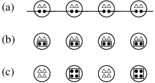
Figure 1: Schematic pictures of (a) the Haldane plateau state, (b) the large-$D$ plateau state, and (c) the Néel plateau state. An $S=2$ spin consists of four $s=1/2$ spins. Big open circles denote $S=2$ spins and small dots $s=1/2$ spins. Open triangles denote $s=1/2$ spins with $s^{z}=1/2$. Solid lines represent singlet dimer pair $(1/\sqrt{2})(|\uparrow\downarrow-\downarrow\uparrow\rangle)$ and rectangles $(1/\sqrt{2})(|\uparrow\downarrow+\downarrow\uparrow\rangle)$. Squares denote the lowest four spin state with $s_{\rm tot}^{z}=0$.

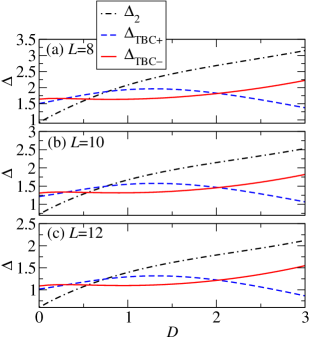
Figure 2: The $D$ dependence of three gaps $\Delta_{2}$ (black dashed-dotted line), $\Delta_{\rm TBC+}$ (blue dashed line), and $\Delta_{\rm TBC-}$ (red solid line) for $\lambda=2.5$ calculated for (a) $L=8$, (b) $L=10$ and (c) $L=12$.

These two plateau phases and the gapless Tomonaga-Luttinger liquid (TLL) phase (no plateau phase) can be distinguished using the level spectroscopy method[4]. According to this analysis, we should compare the following three energy gaps;

$$\Delta_{2}={E(L,M-2)+E(L,M+2)-2E(L,M)\over 2},$$ (4)

$$\Delta_{\rm TBC+}=E_{\rm TBC+}(L,M)-E(L,M),$$ (5)

$$\Delta_{\rm TBC-}=E_{\rm TBC-}(L,M)-E(L,M),$$ (6)

where $E_{\rm TBC+}(L,M)$ ($E_{\rm TBC-}(L,M)$) is the energy of the lowest state with the even parity (odd parity) with respect to the space inversion at the twisted bond under the twisted boundary condition, and other energies are under the periodic boundary condition. The level spectroscopy method indicates that the smallest gap among these three gaps for $M=L=M_{\rm s}/2$ determines the phase at $m=1/2$. Namely, $\Delta_{2}$, $\Delta_{\rm TBC+}$ and $\Delta_{\rm TBC-}$ correspond to the TLL, large-$D$-plateau and Haldane-plateau phases, respectively.

The $D$ dependence of the three gaps calculated for $L=8,10$, and $12$ is plotted for $\lambda=2.5$ in Figs. 2(a), (b), and (c), respectively. These figures indicate that the system is in the no-plateau phase for small $D$, in the Haldane plateau phase for intermediate $D$, and in the large-$D$ plateau phase for large $D$. The system size dependence of the boundary is predicted to proportional to $1/L^{2}$.

Thus assuming the finite-size correction proportional to $1/L^{2}$, we estimate each phase boundary in the infinite length limit from the intersections of the gaps for $L=$8, 10 and 12.

3.2 Translational Symmetry Broken Plateau

If the Ising-like anisotropy $\lambda$ is sufficiently large, the system is expected to exhibit another $m=1/2$ magnetization plateau phase, where the translational symmetry is spontaneously broken like the Néel order, namely $|\cdots,2,0,2,0,\cdots\rangle$. It should be called the Néel plateau phase. The schematic picture of the Néel plateau state is shown in Fig. 1(c). In this phase the excitation with the momentum $k=\pi$ would be degenerate to the lowest state with $k=0$. Thus the phenomenological renormalization is a good method to detect the quantum phase transition to the Néel plateau phase. The lowest excitation gap with $k=\pi$ in the subspace $m=1/2$ is denoted as $\Delta_{\pi}$. The size-dependent fixed point $\lambda_{c}(L+1)$ is determined by the equation

$$L\Delta_{\pi}(L,\lambda)=(L+2)\Delta_{\pi}(L+2,\lambda).$$ (7)

The scaled gap $L\Delta_{\pi}$ for $D=2.0$ is plotted versus $\lambda$ for $L=$6, 8, 10 and 12 in Fig. 3. The size-dependent fixed point $\lambda_{c}(L)$ for $L=$7, 9, 11 is plotted versus $1/L$ for $D=2.0$ in Fig. 5. $\lambda_{\rm c}$ in the infinite length limit is estimated as $\lambda_{\rm c}=4.896\pm 0.004$. The boundary of the Néel plateau phase is estimated by this method.

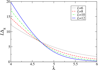
Figure 3: The scaled gap $L\Delta_{\pi}$ for $D=2.0$ is plotted versus $\lambda$ for $L=$6, 8, 10 and 12.

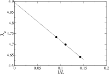
Figure 4: The size-dependent fixed point $\lambda_{\rm c}(L)$ for $L=$7, 9, 11 is plotted versus $1/L$ for $D=2.0$. Assuming the size correction proportional to $1/L$, $\lambda_{\rm c}$ in the infinite length limit is estimated as $\lambda_{\rm c}=4.896\pm 0.004$.

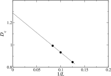
Figure 5: The boundary of the missing region $D_{\rm c}(L)$ for $\lambda=5.0$ is plotted versus $1/L$. Assuming the size correction proportional to $1/L$, $D_{\rm c}$ in the infinite length limit is estimated as $D_{\rm c}=1.286\pm 0.003$.

3.3 Phase diagram

Apart from the gapless (no plateau) and the magnetization plateau phases, there is a parameter region where the $m=1/2$ magnetization is not realized due to the magnetization jump. We think this jump corresponds to the spin flop transition [16, 17] where the Néel order parallel to the external field changes to the quasi-Néel order perpendicular to it. We can find the boundary of this missing region by checking the magnetization curve. Namely, if the $m=1/2$ magnetization is included in the magnetization jump, the system is in the missing region. The boundary of the missing region $D_{\rm c}$ for $\lambda=5.0$ is plotted versus $1/L$ in Fig. 5. Assuming the size correction proportional to $1/L$, $D_{\rm c}$ in the infinite length limit is estimated as $D_{\rm c}=1.286\pm 0.003$. The boundary of the missing region is determined by this method.

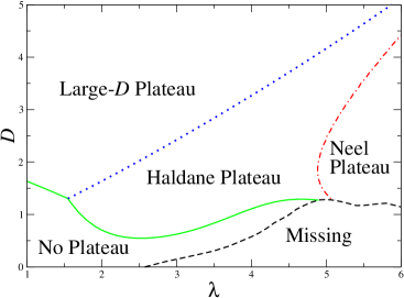
Figure 6: Ground state phase diagram at $m=1/2$ of the present model. It includes the gapless (no plateau), the Haldane, the large-$D$, the Néel plateau phases, and the missing region.

Finally we present the phase diagram at half of the saturation magnetization with respect to the anisotropies $\lambda$ and $D$ shown in Fig. 6. It includes the gapless (no plateau), the Haldane, the large-$D$, the Néel plateau phases, and the missing region. In the Néel plateau phase the translational symmetry is broken.

4 Summary

The $m=1/2$ magnetization state of the $S=2$ antiferromagnetic chain with the anisotropies $\lambda$ and $D$ is investigated using the numerical diagonalization and some finite-size scaling analyses. As a result we found a new $1/2$ magnetization plateau phase with the translational symmetry breaking. The phase diagram at half of the saturation magnetization is presented..

References

- [1] M. Oshikawa, M. Yamanaka and I. Affleck, Phys. Rev. Lett. 78, 1984 (1997).
- [2] E. H. Lieb, T. Schultz and D. J. Mattis, Ann. Phys. (N. Y. ) 16, 407 (1961).
- [3] T. Sakai and M. Takahashi, Phys. Rev. B 57, R3201 (1998).
- [4] A. Kitazawa and K. Okamoto, Phys. Rev. B 62, 940 (2000).
- [5] F. Pollmann, A. M. Turner, E. Berg and M. Oshikawa, Phys. Rev. B 81, 064439 (2010).
- [6] F. Pollmann, E. Berg, A. M. Turner and M. Oshikawa, Phys. Rev. B 85, 075125 (2012).
- [7] T. Sakai, K. Okamoto and T. Tonegawa, Phys. Rev. B 100, 174401 (2019).
- [8] T. Tonegawa, K. Okamoto, H. Nakano, T. Sakai, K. Nomura and M. Kaburagi, J. Phys. Soc. Jpn. 80, 043001 (2011).
- [9] K. Okamoto, T. Tonegawa, H. Nakano, T. Sakai, K. Nomura and M. Kaburagi, J. Phys.: Conf. Ser. 302, 012014 (2011).
- [10] K. Okamoto, T. Tonegawa, H. Nakano, T. Sakai, K. Nomura and M. Kaburagi, J. Phys.: Conf. Ser. 320, 012018 (2011).
- [11] K. Okamoto, T. Tonegawa, T. Sakai and M. Kaburagi, JPS Conf. Proc. 3, 014022 (2014).
- [12] K. Okamoto, T. Tonegawa and T. Sakai, J. Phys. Soc. Jpn. 85, 063704 (2016).
- [13] T. Sakai, T. Yamada, R. Nakanishi, R. Furuchi, H. Nakano, H. Kaneyasu, K. Okamoto and T. Tonegawa, J. Phys. Soc. Jpn. 91, 074702 (2022).
- [14] I. Affleck, T. Kennedy, E. H. Lieb and H. Tasaki, Phys. Rev. Lett. 59, 799 (1987).
- [15] I. Affleck, T. Kennedy, E. H. Lieb and H. Tasaki, Commun. Math. Phys. 115, 477 (1988).
- [16] T. Sakai, Phys. Rev. B 60, 6238 (1999).
- [17] T. Sakai and M. Takahashi, Phys. Rev. B 60, 7295 (1999).