Causal Entropy Optimization

Abstract

We study the problem of globally optimizing the causal effect on a target variable of an unknown causal graph in which interventions can be performed. This problem arises in many areas of science including biology, operations research and healthcare. We propose Causal Entropy Optimization (ceo), a framework which generalizes Causal Bayesian Optimization (cbo) [2] to account for all sources of uncertainty, including the one arising from the causal graph structure. ceo incorporates the causal structure uncertainty both in the surrogate models for the causal effects and in the mechanism used to select interventions via an information-theoretic acquisition function. The resulting algorithm automatically trades-off structure learning and causal effect optimization, while naturally accounting for observation noise. For various synthetic and real-world structural causal models, ceo achieves faster convergence to the global optimum compared with cbo while also learning the graph. Furthermore, our joint approach to structure learning and causal optimization improves upon sequential, structure-learning-first approaches.

1 Introduction

Causal Bayesian Networks (cbns) [49] offer a powerful tool for formulating and testing causal relationships among a set of random variables. Representing a system with a cbn allows one to e.g. estimate causal effects or find interventions optimizing a target node. These tasks often assume, either implicitly or explicitly, exact knowledge of the underlying causal graph. Therefore, structure learning (also called “causal discovery”) from data [22] has received increasing attention in the last few years. In particular, several studies have taken a Bayesian approach by formulating a prior over graphs and selecting interventions to learn the structure via Bayesian Optimal Experimental Design [boed, 46, 60, 43, 26, 33, 47, 63, 19, 64]. Among these studies, a Bayesian Optimization (bo)-based algorithm, targeted at structure learning, has been proposed by von Kügelgen et al. [63] with the goal of reducing the cost of discovering the true graph. A causal bo-based algorithm [cbo, 2] was also recently developed to identify interventions maximizing a target variable, given a known causal graph – a problem named causal global optimization, which we refer to simply as causal optimization. While the two works develop bo algorithms tackling the tasks of structure learning and causal optimization separately, the investigator is often interested in learning optimal actions while not having exact knowledge of the causal relationships among variables. This is the challenging setting we consider in this paper which is the first focusing on solving these two problems jointly.

Example Consider a setting where the investigator aims at finding the level of statin drug or aspirin that should be prescribed to a patient in order to minimize the level of prostate specific antigen (psa).

While the investigator might have a good understanding of the variables affecting the level of psa (see Fig. 1), she might not know the exact causal relationships among them. Therefore, multiple causal graphs might be consistent with her domain knowledge. For instance, the causal relationships between age, body mass index (bmi) and cancer might be known, but those among cancer, psa and different levels of medication administration might be unknown. This is represented by the red edges in Fig. 1. Identifying the optimal drug dosages with cbo would require knowledge of these edges. Indeed, cbo assumes [2, appendix, Fig. 3] them to be oriented as $\{\text{Statin}\rightarrow\text{Cancer},\text{Statin}\rightarrow\textsc{psa},\text{Aspirin}\rightarrow\text{Cancer},\text{Aspirin}\rightarrow\textsc{psa}\}$. We propose Causal Entropy Optimization (ceo), a framework which, instead of assuming a specific causal graph for the data generating process, accounts for the structure uncertainty by employing a Bayesian prior. ceo considers the causal graph prior both in the surrogate models and the acquisition function used within the bo algorithm.

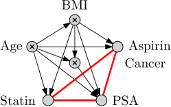
Figure 1: Causal dag with unoriented edges in red. Shaded and crossed nodes represent manipulative and non-manipulative variables respectively. psa is the outcome of interest.

Contributions We make the following contributions:

$\bullet$ We generalize the causal global optimization problem to settings where the graph structure is fully or partially unknown.

$\bullet$ We offer the first solution to this problem which we call Causal Entropy Optimization (ceo). ceo models the causal effects via a set of surrogate models that account for both graph and observation uncertainty.

$\bullet$ We introduce an information-theoretic acquisition function, which we call causal entropy search (ces) that addresses the trade-off between learning the causal graph and identifying the best intervention. ces encompasses existing acquisitions used for bo and experimental design for structure learning as special cases, and could be adapted to solve other active learning tasks.

$\bullet$ We demonstrate across synthetic and real-world causal graphs how accounting for uncertainty leads to faster convergence to the global optimum compared to cbo. In addition, we show how exact knowledge of the causal structure is not always needed for efficient causal global optimization.

2 Background and Problem Statement

We consider a probabilistic causal model [49] consisting of a directed acyclic graph $\mathcal{G}$ (dag) and a four-tuple $\langle\mathbf{U},\mathbf{V},F,p(\mathbf{U})\rangle$, where $\mathbf{U}$ is a set of exogenous background variables distributed according to $p(\mathbf{U})$, $\mathbf{V}$ is a set of observed endogenous variables and $F=\{f_{1},\dots,f_{|\mathbf{V}|}\}$ is a set of functions constituting the structural causal model (scm) such that $v_{i}=f_{i}(pa_{i},u_{i})$ with $\text{pa}_{i}$ denoting the parents of $V_{i}$. Within $\mathbf{V}$, we distinguish between non-manipulative variables $\mathbf{C}$ that cannot be intervened on, continuous treatment variables $\mathbf{X}$ that can be set to specific values and a single output variable $Y$ representing the agent’s outcome of interest – see Fig. 1 for an example. Under the Markov Assumption, each variable $V_{i}$ is conditionally independent of its non-descendants given its parents, such that the joint distribution factorises as: $p(\mathbf{V}\mid\mathcal{G})=\prod_{V_{j}\in\mathbf{V}}p(V_{j}\mid\mathbf{Pa}_{j}^{\mathcal{G}},\mathcal{G})$. Denote by $\mathcal{P}(\mathbf{X})$ the power set of $\mathbf{X}$ giving all possible interventions we can perform in the graph. The set $\mathbf{X}_{I}\in\mathcal{P}(\mathbf{X})$ represents one such intervention set with $\mathbf{V}_{I}=\mathbf{V}\setminus\mathbf{X}_{I}$ being the corresponding set of non-intervened variables. We assume causal sufficiency [52] and perfect interventions [50] so that, for any set $\mathbf{X}_{I}$, the interventional distribution $p(\mathbf{V}_{I}\mid\text{do}(\mathbf{X}_{I}=\mathbf{x}_{I}))$ resulting from setting $\mathbf{X}_{I}$ to a value $\mathbf{x}_{I}$ obeys the following truncated factorization:

$$p(\mathbf{V}_{I}\mid\text{do}(\mathbf{X}_{I}=\mathbf{x}_{I}),\mathcal{G})=\prod_{V_{j}\in\mathbf{V}_{I}}p(V_{j}\mid\mathbf{Pa}_{j}^{\mathcal{G}})\Bigr{|}_{\mathbf{X}_{I}=\mathbf{x}_{I}}$$

where the vertical line represents evaluation of the expression at $\mathbf{X}_{I}=\mathbf{x}_{I}$.
Notation Note that, throughout, lowercase denotes realizations of random variables (r.v.), while uppercase denotes the r.v. We denote collected data by $\mathcal{D}=\{\{(\mathbf{x}_{I}^{(i)},\mathbf{v}_{I}^{(i)})\}_{i=1}^{N}\}_{\mathbf{X}_{I}\in\textsc{{es}}}$ where the exploration set (es) is $\textsc{{es}}=\mathcal{P}(\mathbf{X})$ or $\textsc{{es}}\subseteq\mathcal{P}(\mathbf{X})$ if only a subset of interventions can be implemented in the system (e.g. if $\mathcal{P}(\mathbf{X})$ is too large). Here, $\mathbf{v}_{I}^{(i)}$ represents one set of values of the non-intervened variables $\mathbf{V}_{I}$ in a mutilated graph where $\mathbf{X}_{I}$ is set to $\mathbf{x}_{I}^{(i)}$. Further, $\mathbf{v}_{I}^{(i)}$ includes both a value for the target variable $y^{(i)}$ and a value for the remaining variables, denoted by $\mathbf{v}_{I_{Y}}^{(i)}=\mathbf{v}_{I}^{(i)}\setminus y^{(i)}$. The dataset $\mathcal{D}$ includes all data, that is observational data ($\mathcal{D}^{O}$) which correspond to $I=\varnothing$ and interventional data ($\mathcal{D}^{I}$). Every time we intervene in the system we collect $N>1$ samples from each interventional distribution, but the framework equally handles $N=1$. See App. Section A for a table describing the full notation.

Problem statement We consider the causal global optimization problem introduced by Aglietti et al. [2] and generalize it to settings with an unknown causal graph. Given $\mathcal{D}$, we seek to identify the interventional set and corresponding values optimizing the causal effect in the true causal graph $\mathcal{G}$:

$$\mathbf{X}_{I}^{\star},\mathbf{x}_{I}^{\star}=\underset{\begin{subarray}{c}\mathbf{X}_{I}\in\mathcal{P}(\mathbf{X})\\ \mathbf{x}_{I}\in D\left(\mathbf{X}_{I}\right)\end{subarray}}{\operatorname*{arg\,min}}\mathbb{E}[Y\mid\text{do}(\mathbf{X}_{I}=\mathbf{x}_{I}),\mathcal{G}]\text{,}$$ (1)

where $D\left(\mathbf{X}_{I}\right)$ denotes the interventional domain of $\mathbf{X}_{I}$ and the causal effect depends on the true graph $\mathcal{G}$. Solving the problem in Eq. 1 is challenging as evaluating $\mathbb{E}[Y\mid\text{do}(\mathbf{X}_{I}=\mathbf{x}_{I}),\mathcal{G}]$ requires intervening in the real system at a cost, which we assume to be given by $\textsc{Co}(\mathbf{X}_{I},\mathbf{x}_{I})$. While Eq. 1 is the objective of cbo, since the graph is unknown the problem becomes more challenging.

Remark: Notice that, when the graph is known, one can solve the problem in Eq. 1 resorting to cbo. When the graph is unknown, there is no existing unified solution for the problem. This paper offers such a solution and shows how, accounting for graph uncertainty, one can match the performance of cbo, which requires knowledge of the true graph, in terms of convergence speed to the optimum.

3 Methodology

There are three main ingredients to our solution to the problem in Eq. 1: a set of surrogate models for the causal effects on the target node (Section 3.1) accounting for different sources of uncertainty, a posterior over the graph structure (Section 3.2), computed exploiting observational and interventional data, and an information-theoretic acquisition function (Section 3.3) balancing the trade-off between optimization and structure learning. We now detail each ingredient and provide the pseudocode for ceo in Algorithm 1.

3.1 Inference on the causal effects

Prior Surrogate Models For each set $\mathbf{X}_{I}\in\textsc{{es}}$ we place a Gaussian process [gp, 68] prior on $f_{I}(\mathbf{x}_{I})=\mathbb{E}[Y\mid\text{do}(\mathbf{X}_{I}=\mathbf{x}_{I}),\mathcal{G}]$ and construct a prior mean and kernel function that incorporates our current belief about the graph together with the observational and interventional data. Specifically, we define $f_{I}(\mathbf{x}_{I})\sim\mathcal{GP}(m_{I}(\mathbf{x}_{I}),k_{I}(\mathbf{x}_{I},\mathbf{x}_{I}^{\prime}))$ with:

$$m_{I}(\mathbf{x}_{I})=\widehat{\mathbb{E}}[Y\mid\text{do}(\mathbf{X}_{I}=\mathbf{x}_{I})]\qquad k_{I}(\mathbf{x}_{I},\mathbf{x}_{I}^{\prime})=k(\mathbf{x}_{I},\mathbf{x}_{I}^{\prime})+\widehat{\mathbb{V}}[Y\mid\text{do}(\mathbf{X}_{I}=\mathbf{x}_{I})],$$ (2)

where $k(\cdot,\cdot)$ is a problem-dependent kernel function of choice. As in the surrogate model of cbo, we set $m_{I}$ as an empirical estimate of the underlying true function using observational data. However, here we additionally incorporate the uncertainty over the graph by introducing latent variable $G$:

$$\widehat{\mathbb{E}}[Y\mid\text{do}(\mathbf{X}_{I}=\mathbf{x}_{I})] =\mathbb{E}{\left[\hat{\mathbb{E}}{\left[Y|\text{do}(\mathbf{X}_{I}=\mathbf{x}_{I}),G\right]}\right]}$$ (3)

$$\widehat{\mathbb{V}}[Y\mid\text{do}(\mathbf{X}_{I}=\mathbf{x}_{I})] =\mathbb{E}{\left[\hat{\mathbb{V}}[Y\mid\text{do}(\mathbf{X}_{I}=\mathbf{x}_{I}),G]\right]}+\mathbb{V}[\hat{\mathbb{E}}{\left[Y\mid\text{do}(\mathbf{X}_{I}=\mathbf{x}_{I}),G\right]}]\text{,}$$ (4)

where outer expectations/variances are w.r.t a probability mass function on the r.v. $G$, i.e. $P(G)$; $\hat{\mathbb{E}}$ denotes that the expectation involves some approximation. Here, the approximation arises because we use $\hat{p}(Y\mid\text{do}(\mathbf{X}_{I}=\mathbf{x}_{I}),G=g)$, an estimate of the interventional distribution computed via the do-calculus with only observational data . Note that, when collecting data, $P(G)$ will be replaced by $P(G\mid\mathcal{D})$, which also includes interventions. Thus, our models combine observational and interventional data. Computing this posterior will be discussed in detail in Section 3.2.

Surrogate Model Likelihood For each intervention set $\mathbf{X}_{I}\in\textsc{{es}}$ and value $\mathbf{x}_{I}^{(i)}$, we assume the output $y$ to be a noisy realisation of the objective function $y=f_{I}(\mathbf{x}_{I})+\nu$ at $\mathbf{x}_{I}^{(i)}$ where $\nu\sim\mathcal{N}(0,s^{2})$. Indeed, every time we perform $\text{do}(\mathbf{X}_{I}=\mathbf{x}_{I}^{(i)})$, we obtain a single sample $\mathbf{v}_{I}^{(i)}$ from the resulting interventional distribution $p(\mathbf{V}_{I}|\text{do}(\mathbf{X}_{I}=\mathbf{x}_{I}^{(i)}),\mathcal{G})$. Noisy observations were not considered by cbo, which made a simplifying assumption, and complicate the identification of the optimal intervention.

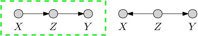
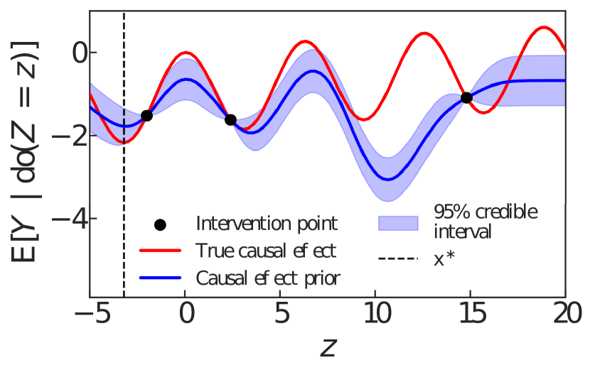
(a)

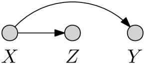
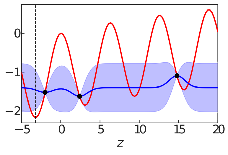
(b)

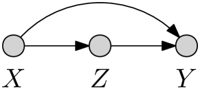
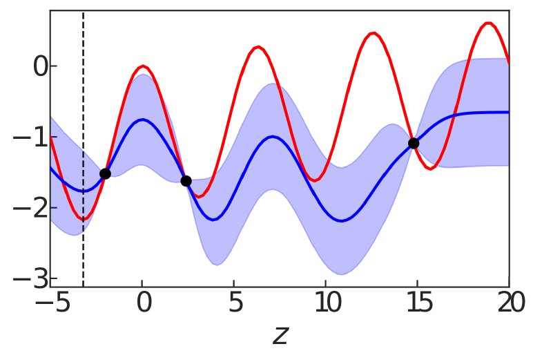
(c)

Figure 2: Each figure plots the true underlying causal effect function $\mathbb{E}[Y\mid\text{do}(Z=z),G=\mathcal{G}]$ in red, while showing different surrogate models arising from Eq. 3 and Eq. 4 when assuming each of the graphs of top of the plot is the correct one. The surrogate models share hyper-parameters so the differences only stems from alternative causal assumptions. The true dag $\mathcal{G}$ is shown inside the dashed box in Fig. 2(a). Vertical dashed line indicates the global optimum. Note that both the true graph and the second dag above (a) result in the same surrogate model.

Posterior Surrogate Models Given the Gaussian likelihood, the posterior distribution $p(f_{I}\mid\mathcal{D})$ can be derived analytically and will also be a gp with mean $m_{I}(\mathbf{X}\mid\mathcal{D})$ and covariance functions $k_{I}(\mathbf{x}_{I},\mathbf{x}_{I}^{\prime}\mid\mathcal{D})$ computed by standard gp updates [68, p. 19].

3.2 Inference on the causal graph

Given $\mathcal{D}$, we update the prior distribution on $G$ to get $P(G\mid\mathcal{D})$, so that we can account for the updated uncertainty in the surrogate models.

We follow the setting of von Kügelgen et al. [63], considering a discrete uniform prior distribution on $G$ with $P(G=g)=\frac{1}{|R_{G}|}$, and graphs can be enumerated. This is appropriate for intended applications of cbo, where a manageable number of graphs representing alternative causal hypotheses is maintained. However, we note that in our framework only expectations of the graph posterior are required.

Graph Likelihood In order to define the graph likelihood,we assume an additive noise model with i.i.d. Gaussian noise terms. For every $g$ and $X_{j}\in\mathbf{X}$, we have:

$$X_{j}=f_{j}(\mathbf{Pa}_{j}^{G=g})+\epsilon_{j},\;\;f_{j}\mid(\mathbf{Pa}_{j}^{G=g}=\mathbf{x},\theta_{j})\sim\mathcal{GP}(0,k_{j}(\mathbf{x},\mathbf{x}^{\prime};\theta_{j}))$$ (5)

with $\epsilon_{j}\sim\mathcal{N}(0,\sigma^{2}_{j})$ and where $\theta_{j}$ represents a set of hyper-parameters. Further, $\mathbf{x}$ and $\mathbf{x}^{\prime}$ are two values for the parents of $V_{j}$ in $G=g$ and $k_{j}$ is a kernel function of choice. Exploiting the available data we can then compute $p(f_{j}\mid\mathbf{Pa}_{j}^{G},\mathcal{D}^{O})$ in closed form. Hence, each term in the truncated factorization is a gp marginal likelihood (details in App. Section B.)

Graph Posterior Given the prior distribution on $G$ and the likelihood, we can compute the posterior distribution on $G$ in closed form as $P(G\mid\mathcal{D})\propto p(\mathcal{D}|G)P(G)$ due to the tractability of gps. Importantly, this also allows us to compute the expectations w.r.t. $P(G|\mathcal{D})$ without approximations in both Eqs. 3 and 4 and later in the acquisition function. Regarding convergence to $\delta_{G=\mathcal{G}}$, the key requirements needed are: causal sufficiency; that $R_{G}$ includes $\mathcal{G}$; all variables can be manipulated; infinite samples can be obtained from each node; causal minimality. See Appendix B for details.

Effect of graph knowledge on optimization It is important to emphasize that while computing $P(G\mid\mathcal{D})$ and using it in the surrogate model provides proper uncertainty quantification, exact knowledge of the causal structure is not always needed for more efficient causal optimization.

Indeed, different graphs may lead to equivalent surrogate models. For instance, consider the example in Fig. 2 showing different causal graphs and the associated surrogate models, when three interventions are collected. Here the true dag is given in Fig. 2(a) (green dashed box) alongside an alternate causal dag. The surrogate models for these structures are equivalent, and shown in the plot below. Indeed, the do-calculus for the left dag and right dag of Fig. 2(a) gives the same result, even if the latter dag is wrong. Given our surrogate model construction in (Eq. 2), this implies the same prior mean and covariance for the causal effects associated with both graphs. Therefore, for the purpose of causal optimization, the dags in Fig. 2(a) are the same.

As demonstrated experimentally in Section 5, it is thus wasteful to intervene to find the true graph first, and only after perform causal optimization. This motivates our joint approach, which automatically balances structure learning and optimization by picking interventions that are reducing the uncertainty of $P(G\mid\mathcal{D})$ when doing so enables faster identification of the optimum. Next, we describe how to achieve this balance by proposing a new acquisition function.

3.3 Acquisition function: Causal Entropy Search

We propose an acquisition function that combines Bayesian structure learning and causal optimization into a single objective in order to balance the two tasks. To do so, we start by framing the tasks of causal optimization and structure learning, respectively, as gaining information about the global optimum value $y^{\star}=\min(\text{or}\max)_{I}y^{\star}_{I}$ and about $G$. This information gain can be quantified by considering the reduction in uncertainty in an appropriately defined joint distribution on $y^{\star}$ and $G$. While a distribution on the graph, $P(G\mid\mathcal{D})$, was defined in Section 3.2, the distribution on $y^{\star}$ is implicitly induced by the surrogate models defined in Section 3.1.

Our acquisition is thereby defined as the conditional mutual information (mi) denoted by $\mathbb{I}(\cdot;\cdot\mid\cdot)$ between the random variables $(y^{\star},G)$ and the outcome of the experiment $\left(\mathbf{v}_{Y},y\right)$, given data $\mathcal{D}$. An experiment in the context of a causal dag consists of performing $\text{do}(\mathbf{X}_{I}=\mathbf{x}_{I})$ and observing a sample $\mathbf{v}_{I}=(y,\mathbf{v}_{Y})$ from the resulting interventional distribution. Therefore, in ceo we seek an intervention set $\mathbf{X}_{I}^{\text{best}}$ and corresponding value $\mathbf{x}_{I}^{\text{best}}$ such that:

$$\mathbf{X}_{I}^{\text{best}},\mathbf{x}_{I}^{\text{best}} =\operatorname*{arg\,max}_{\mathbf{X}_{I}\in\textsc{{es}},\leavevmode\nobreak\ \mathbf{x}_{I}\in D\left(\mathbf{X}_{I}\right)}\alpha_{\textsc{ceo}}(\mathbf{X}_{I},\mathbf{x}_{I})$$

$$\alpha_{\textsc{ceo}}(\mathbf{X}_{I},\mathbf{x}_{I}) =\frac{\mathbb{I}\left[\left(y^{\star},G\right);\left(\mathbf{X}_{I},\mathbf{x}_{I},\mathbf{v}_{Y},y\right)\mid\mathcal{D}\right]}{\textsc{Co}(\mathbf{X}_{I},\mathbf{x}_{I})}$$ (6)

where the denominator $\textsc{Co}(\mathbf{X}_{I},\mathbf{x}_{I})$ provides the mi per unit of cost. We call the acquisition function in Eq. 6 Causal Entropy Search (ces).

Assume, for the moment, that we have access to $p(y^{\star},G)$ and the associated posterior. We write its joint entropy as:

$$\mathbb{H}[p(y^{\star},G\mid\mathcal{D})]=-\sum_{G}\int\mathrm{d}y^{\star}p(G,y^{\star}\mid\mathcal{D})\log p(G,y^{\star}\mid\mathcal{D})\text{.}$$ (7)

The work in [42, Lemma 2.3 and Eq. 2.2] shows that conditional MI and joint entropies can be rigorously defined in an analogue way to their fully continuous/discrete counterparts. The book [12] gives conditions on densities required for the differential entropy to exist and be bounded. We can then use Eq. 7 to evaluate the numerator of ces, i.e. Eq. 6, which can be written as:

$$\mathbb{E}_{p(\mathbf{v}_{Y},y\mid\text{do}(\mathbf{X}_{I}=\mathbf{x}_{I}),\mathcal{D})}\Big{[}\mathbb{H}[p(y^{\star},G\mid\mathcal{D})]-\mathbb{H}[p(y^{\star},G\mid\mathcal{D}\cup\left(\mathbf{x}_{I},\mathbf{v}_{Y},y\right))]\Big{]}\text{.}$$

This is the reduction in entropy observed on average in the joint distribution on $(y^{\star},G)$ when performing $\text{do}(\mathbf{X}_{I}=\mathbf{x}_{I})$ and observing $\mathbf{v}_{Y}=(\mathbf{v}_{Y},y)$. We note that computing this term does not require intervening in the real system. For a given intervention we “fantasize” (a concept often used in bo [69]) about the outcomes $\mathbf{v}_{Y}$ we would get by simulating what would happen in the system under $\text{do}(\mathbf{X}_{I}=\mathbf{x}_{I})$. This can be done in ceo by using the surrogate models and the fitted scm functions. Note that this formulation automatically takes into account noisy observations, which often motivates entropy-based acquisitions in bo [17]. We now discuss how to define and obtain $p(y^{\star},G)$, and approximate $\mathbb{H}[p(y^{\star},G)]$.

Table 1: Causal Entropy Search compared to related objectives in boed for structure learning and bo algorithms. Entropy Search (es) and Max-value es are used within the standard a-causal bo problem. Multi-Task bo is also used for a-causal optimization with multiple functions, but when the function containing the optimum is known. The objective in [63] is also based on mi, but only targets the graph structure. ces considers intervention sets, intervention values and the graph structure when the function containing the optimum is unknown.

Acquisition	Objective
ces (ours)	$\frac{\mathbb{I}\left[\left(y^{\star},G\right);\left(\mathbf{X}_{I},\mathbf{x}_{I},\mathbf{v}_{Y},y\right)\mid\mathcal{D}\right]}{\textsc{Co}(\mathbf{X}_{I},\mathbf{x}_{I})}$
Entropy Search [29]	$\mathbb{I}\left[(\mathbf{x},y);\mathbf{x}^{\star}\right|\mathcal{D}]$
Max-value Entropy Search [66]	$\mathbb{I}\left[(\mathbf{x},y);y^{\star}\right|\mathcal{D}]$
Multi-Task bo [59]	$\frac{\mathbb{I}\left[(\mathbf{x}^{\text{task}},y);\mathbf{x}^{\star}\right|\mathcal{D}]}{\textsc{Co}(\text{task})}$
Causal discovery via bo [63]	$\mathbb{I}\left[G;\left(\mathbf{X}_{I},\mathbf{x}_{I},\mathbf{v}_{I}\right)\mid\mathcal{D}\right]$

Algorithm 1 ceo

1:Input: $\mathcal{D}$, $P(G)$, $H$ (N. of iterations)

2:Output: $\mathbf{X}_{I}^{\star},\mathbf{x}_{I}^{\star},P(G\mid\mathcal{D}_{H})$.

3:Initialise: Set $\mathcal{D}_{0}=\mathcal{D}$.

4:Compute $p(\mathcal{D}_{0}\mid G=g)$ for each $g\in R_{G}$.

5:Compute $P(G\mid\mathcal{D}_{0})$.

6:Compute $m_{I}(\mathbf{x}_{I})$ and $k_{I}(\mathbf{x}_{I},\mathbf{x}_{I}^{\prime})$ using the do-calculus for each $\mathbf{X}_{I}\in\textsc{{es}}$ (Eq. 3 and Eq. 4).

7:for $h=1,...,H$ do

8:   Compute $\alpha_{\textsc{ceo}}(\mathbf{X}_{I},\mathbf{x}_{I})$ for each $\mathbf{X}_{I}\in\textsc{{es}}$ and each $\mathbf{x}_{I}$ in the acquisition points with ces (Algorithm 2 in App.).

9:   Obtain the optimal set-value pair $(\mathbf{X}_{I}^{h},\mathbf{x}_{I}^{h})$.

10:   Intervene on the system and augment the dataset $\mathcal{D}_{h}=\mathcal{D}_{h-1}\cup(\mathbf{x}_{I}^{h},\mathbf{v}_{I}^{h})$.

11:   Compute $P(G\mid\mathcal{D}_{h})$ and every $p(f_{I}\mid\mathcal{D}_{h})$.

12:end for

13:Return $(\mathbf{X}_{I}^{\star},\mathbf{x}_{I}^{\star}),P(G|\mathcal{D}_{H})$

Joint posterior over $y^{\star}$ and $G\leavevmode\nobreak\ \leavevmode\nobreak\$ Computing ces requires defining $p(y^{\star},G)$, obtaining its posterior given $\mathcal{D}$ and computing Eq. 7. We model the joint distribution as $p(y^{\star},G\mid\mathcal{D})=P(G\mid y^{\star},\mathcal{D})p(y^{\star}|\mathcal{D})$. We can thus write Eq. 7 as the sum of: $-\sum_{G}\int\mathrm{d}y^{\star}P(G\mid y^{\star},\mathcal{D})p(y^{\star}\mid\mathcal{D})\log P(G\mid y^{\star},\mathcal{D})$ and $\mathbb{H}(p(y^{\star}\mid\mathcal{D}))$. In turn, evaluating these two terms require computing $P(G\mid y^{\star},\mathcal{D})$ and sampling from $p(y^{\star}\mid\mathcal{D})$. The former can be achieved by updating the posterior on $G$ to get $P(G\mid\mathcal{D}\cup(\mathbf{x}^{\star},\mathbf{v}_{Y}^{\star},y^{\star}))$ and marginalizing over $\mathbf{x}^{\star}$ and $\mathbf{v}_{Y}^{\star}$ (see App. Section C.1 for details).

However, since $p(y^{\star}\mid\mathcal{D})$ is not in available closed form, and a simple Monte Carlo approximation is computationally expensive, we propose a heuristic approximation that works in practice. Specifically, we approximate the distribution of $y^{\star}$ to be a mixture of the intervention-specific distributions on the optimal targets, where the weights are given by the probability of each intervention set being optimal:

$$p(y^{\star}\mid\mathcal{D})=\sum_{y_{I}^{\star}:\mathbf{X}_{I}\in\textsc{{es}}}P(\mathbf{X}_{I}=\mathbf{X}^{\star})\leavevmode\nobreak\ p(y_{I}^{\star}\mid\mathcal{D}),$$ (8)

where $\mathbf{X}^{\star}$ is the intervention set in es which yields the global optimum. We can thus sample from Eq. 8 via standard mixture sampling techniques [48]. Notice that Eq. 8 is accounting for the fact that we do not know which intervention set and thus surrogate model is associated with the global optimum. See Table 1 for connections between the ces and related existing objectives.
Motivation of posterior approximation Notice that as we collect data and get closer to the optimum, we expect the weights of the mixture distribution Eq. 8 gradually concentrate around the optimal intervention set $\mathbf{X}^{\star}$, and $p(y^{\star}\mid\mathcal{D})$ turns into $p(y_{I}^{\star}\mid\mathcal{D})$ for the $\mathbf{X}_{I}$ s.t. $\mathbf{X}_{I}=\mathbf{X}^{\star}$. To model the belief over the optimal set $P(\mathbf{X}_{I}=\mathbf{X}^{\star})$, we employ a multi-armed bandit [38] perspective and define the weights via an upper confidence bound (UCB) policy – see App. Section H for details.
Computational complexity Let $N$ be the number of acquisition points i.e., given $\mathbf{X}_{I}$, we will consider $\{\mathbf{x}_{I}^{(n)}\}_{n=1}^{N}$ as candidate values to compare with ces. The total complexity of ces can be written: $\mathcal{O}(N\cdot\text{CES}(\mathbf{x})\cdot\sum_{\mathbf{X}_{I}\in\mathbf{ES}}|\mathbf{X}_{I}|)$. Here, $\text{CES}(\mathbf{x})$ denotes the time needed to compute ces for m specific value $\mathbf{x}$, regardless of its corresponding $\mathbf{X}_{I}$. Note this is valid for CBO also, replacing $\text{CES}(\mathbf{x})$ with $\text{CEI}(\mathbf{x})$, the acquisition used by CBO [2]. Here, $\text{CES}(\mathbf{x})$ involves approximating univariate marginals $p(y_{I}^{\star}\mid\mathcal{D})$ and the mixture Eq. 8. We do this with Kernel Density Estimation (KDE); the complexity of these operations depend on the accuracy needed to estimate these marginals. Finally, since the number of graphs in our setting is tractable, we can compute expectations w.r.t $P(G)$ without approximations and with negligible cost w.r.t to the rest.

4 Related work

Causal Effect Estimation A variety of approaches to estimate causal effects from observational data have been proposed, including those based on propensity scores [51], instrumental variables [6] or scms [49]. On the contrary, there have been few methods combining interventional and observational data [54]. Focusing on scm methods, apart from a few exceptions [31, 30], causal effects are estimated assuming exact knowledge of $\mathcal{G}$.

Causal Discovery The majority of causal discovery (cd) methods focus on learning $\mathcal{G}$ using only observational data thus restricting the identification to the Markov equivalence class (mec) [61, 5, 56, 9, 18, 53, 32, 74]. The seminal work by Cooper and Yoo [11] first showed how experimental design can improve causal structure learning (which in general is known to be NP-hard [8]). Since this study, several papers have focused on learning $\mathcal{G}$ from a combination of interventional and observational data [60, 46, 15, 25, 26, 27, 66, 47, 70, 21, 4, 16]. However, all of these focus on finding the true graph by selecting the intervention set only. Our work additionally selects intervention values. Recently, von Kügelgen et al. [63] developed a bo framework for cd where variables are continuous and follow flexible non-linear relationships.

Optimal Causal Decision Making The literature on causal decision making has mainly focused on finding the optimal treatment regime using observational data [72, 7, 24]. The idea of identifying the optimal action or policy by performing interventions in a causal system has been explored in causal bandits [37], causal reinforcement learning [73] and, more recently, in bo [2, 1, 3]. Importantly, all these approaches assume exact knowledge of the causal relationships beforehand, an assumption that is often not met in practice. Recent work attempts to relax this for causal bandits [39, 65].

Entropy in Causality The use of information-theoretic concepts such as entropy in a causal setting has been receiving increased interest. Kocaoglu et al. [34] introduces the framework “Entropic Causal Inference’, which exploits an entropy condition on a exogenous variable to find the causal direction between two categorical nodes from observational data (extended in [10]); a related notion, “common entropy”, for two discrete random variables is discussed in [35] which improves classic causal discovery algorithms such as PC and FCI. The works [58, 44] discuss the use of entropy among more than two variables.

5 Experiments

We demonstrate ceo on a benchmark synthetic example used in [2] as well as real-world applications for which a dag is available and can be used as a simulator. Without loss of generality, we will always minimize causal effects rather than maximize. Results are averaged over 12 replicates of different initial $\mathcal{D}^{I}$, while $\mathcal{D}^{O}$ is fixed. We set $|\mathcal{D}^{I}_{0}|=2$ and $|\mathcal{D}^{O}_{0}|=200$ (initial data) unless otherwise specified. Full experimental details including scm details, kernel functions used, hyper-parameter optimization can be found in Section K of the supplement. As a reminder for key notation, recall $\mathcal{G}$ denotes the true causal graph; $y^{\star}$ denotes the best value of the causal effect across $\mathbf{ES}$.

Experiments Roadmap & Baselines We compare the performance of ceo against cbo which is the state-of-the-art algorithm addressing the causal global optimization problem. However, as cbo assumes knowledge of the graph, we run it first assuming the true graph $\mathcal{G}$ and then assuming each of the wrong graphs. In general, cbo with $\mathcal{G}$ is expected to perform better, especially when the graph structure is particularly informative for the cbo prior. However, this need not be the case in all experiments. Indeed, in one of our real examples, cbo equipped with $\mathcal{G}$ performs worse than ceo. To further highlight the benefit of our joint method, in Section 5.2 we compare against an algorithm that first identifies the causal graph by optimizing the mi as considered by von Kügelgen et al. [63], and then runs cbo to select the optimal action retaining the interventional data collected when learning about the graph. This is to show that jointly considering structure learning and causal optimization leads to better performance than a sequential approach. We refer to this method as cd-cbo. Notice that we cannot compare directly to von Kügelgen et al. [63] as in their work the mi is optimized via bo rather than computed as in ceo. Finally, notice also that causal discovery methods which do not (1) collect interventions with active learning (2) select both intervention sets and values and (3) assume continuous variables, are not applicable to the problem setting thus we do not consider them as an alternative to von Kügelgen et al. [63] for cd-cbo.

Performance measures

Table 2: Average gap $\pm$ one standard error computed across 12 replicates initialized with different $\mathcal{D}$. Higher values are better, and $0\leq$ gap $\leq 1$. The best result for each experiment in bold.

Method	Synthetic (Fig. 2(a))	Health (Fig. 1)	Epi (Fig. 4)	$\text{Epi}^{+}$ (Fig. 9 App. J)
ceo	$\textbf{0.75}\pm 0.03$	$0.62\pm 0.07$	$\textbf{0.59}\pm 0.06$	$\textbf{0.65}\pm\textbf{0.03}$
cbo w. $G=\mathcal{G}$	$0.66\pm 0.04$	$\textbf{0.71}\pm 0.05$	$0.50\pm 0.05$	$0.50\pm 0.03$
cbo w. $G\neq\mathcal{G}$	$0.59\pm 0.03$	$0.62\pm 0.06$	$0.50\pm 0.06$	$0.53\pm 0.03$

We evaluate performance by assessing the convergence speed to the optimum value of $Y$ as measured by the total cumulative cost of interventions taken where the cost of a single intervention is given by the number of variables in the intervened set. Further, we also evaluate our approach using the gap metric introduced in Aglietti et al. [3, Eq. (4)]. Note that $0\leq\textsc{gap}\leq 1$ and that higher values are better.

5.1 Synthetic example

We start by considering data generated by the chain graph $X\rightarrow Z\rightarrow Y$ as per Fig. 2(a) (green dashed box). We consider all possible alternative dags with three nodes as alternative causal hypotheses, except for those which do not make sense for causal optimization: graphs with any isolated nodes or where the target $Y$ is not a sink. See App. Section I for the full list of graphs and the true scm.

Convergence results are given in Fig. 3, while we show the evolution of the posterior on the true graph over iterations in App. Section D. Note how cbo run under incorrect causal assumptions does not converge to the global optimum, whereas ceo matches the performance of cbo run with the true graph even if the graph posterior has not converged. This is confirmed by the gap values in Table 2 where ceo outperforms both cbo algorithms across 12 replicates.

5.2 Comparison with learning the structure first, then performing cbo (cd-cbo)

We now study how ceo compares against an algorithm that first performs causal discovery and, once the graph has been identified, solves the optimization problem via cbo. We refer to this as cd-cbo. We consider the graph learned once it has more than $90\%$ of posterior mass. In Fig. 3(a) , notice the significantly worse performance at optimization of cd-cbo. This is due to the fact that, while the mi correctly identifies $\mathcal{G}$ after a few samples for most graphs, the graph in Fig. 2(c) is very hard to distinguish from $\mathcal{G}$ (for the given scm) as the terms in the truncated factorization give similar likelihood values. Therefore, the posterior never gets concentrated around a single graph despite the high number of selected interventions, and the optimization task is never solved. This reflects the benefit of a joint approach, where the graph is learned along optimization of the effect, and only to the extent to which it is useful for optimization. Additional results are presented in Appendix N.

5.3 Real examples

We now study the performance of ceo with causal dags used in two real-world settings: one in healthcare to model the level of Prostate Specific Antigen (psa) and one in epidemiology to model the level of hiv virus load. These graphs exhibit a significantly more complex dependency structure than the chain graph of the synthetic example. For the graphs considered here, we found our posterior to converge immediately as soon as initial data $\mathcal{D}$ is provided, or after one/two interventions. ceo can take advantage of this, and simply optimize the mi for $y^{\star}$.

Healthcare The scm for this real-world application results in causal effects that are linear functions of their inputs, observed with standard white Gaussian noise. We designed four incorrect graphs which represent plausible hypotheses a doctor may have in this context (App. Section K). Due to the simplicity of the underlying true functions, one can see that the greediness of ei (used by cbo) grants it better performance on average. ceo still consistently outperforms cbo on the wrong graphs. This also shows evidence that while exact knowledge of the graph is not always required for efficient optimization, it can be better on average than incorrect knowledge of it.

Epidemiology In this example, adapted from [28], the goal is to subministrate doses for two potential treatments, which we denote as $T$ and $R$, (see [28] for details) to minimize HIV viral load. The associated dag is shown in Fig. 4. Fig. 3(c) shows how, in this more challenging scenario, both competitor methods perform worse. Indeed, the multimodal nature of the causal effects and the high observation noise characterizing this example penalise cbo and its ei acquisition function, which is known to be more greedy than entropy based one [17]. While this has been observed in a-causal bo, it is even more problematic when exploring and comparing multiple functions as in cbo.

Extended Epidemiology: To conclude, we test the algorithm on a larger graph obtained by adding confounders to the Epidemiology dag. The resulting dag includes 10 nodes, and the associated wrong graphs are created by removing the same edges from the original graph as in the Epidemiology experiment. Even under this situation, as in the previous Epidemiology experiment, we find that ceo generally performs better than cbo (with both wrong and true). Indeed, a larger graph implies a larger product in the truncated factorization term; this can imply further overconfidence in the cbo surrogate model, whereas ceo averages over multiple plausible hypotheses.

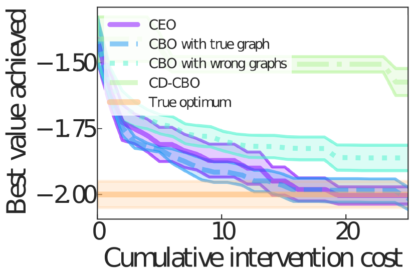
(a) Synthetic.

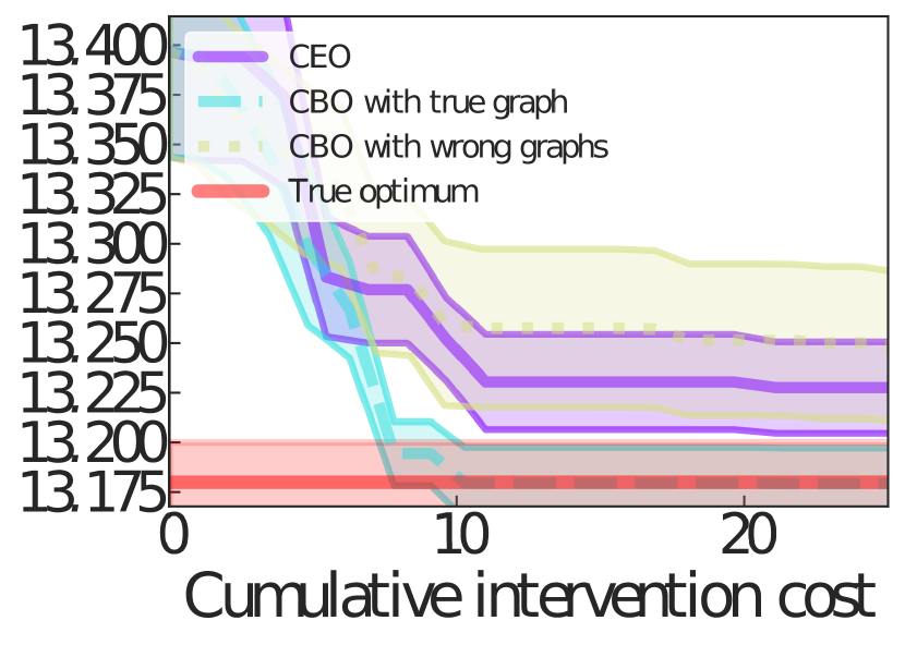
(b) Healthcare.

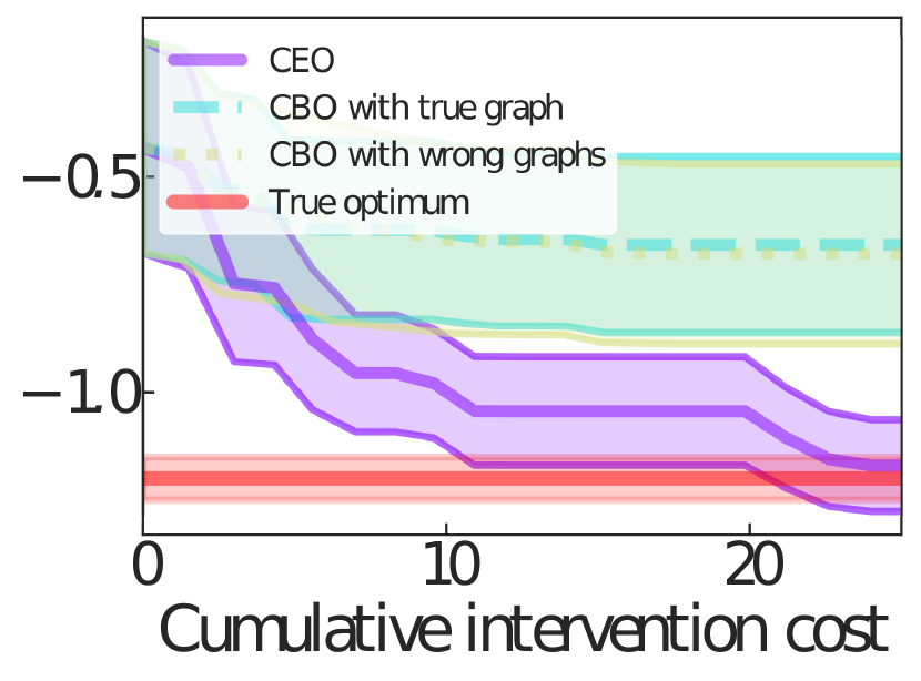
(c) Epidemiology.

(d) Ext. Epidemiology

Figure 3: Convergence plot for ceo and competitor methods across replicates. In the Healthcare and Epidemiology examples, the graph is found immediately by the posterior with the initial $\mathcal{D}^{O}$ and $\mathcal{D}^{I}$; therefore cd-cbo simply reduces to cbo. Shaded areas are $\pm$ one standard error. We plot $\pm 0.05$ around the global optimum shaded in red. Vertical axis shows best value of the causal effect achieved, horizontal shows cumulative intervention cost.

6 Discussion & Conclusions

Figure 4: True dag used for the epidemiology experiment. For the full support of $P(G)$, and scm equations, see App. Section J. Crossed variables are non-manipulative.

We proposed ceo, a framework that allows an experimenter to efficiently solve the causal global optimization problem when the graph is unknown. ceo handles continuous variables with flexible nonparametric relationships, while still allowing for a closed-form posterior over graphs that combines observational and interventional data. Our experiments with synthetic and real-world dags show that ceo allows the experimenter to reach the global optimum with significantly reduced cost compared to cbo when the graph is unknown, and sometimes even when the graph is known. Our acquisition, ces, allows to learn the graph only to the extent to which it is useful for optimization, and it is robust to observation noise.

A limitation of ceo is its restriction to continuous variables, which inherits from cbo. Further, a significant computational effort is required to efficiently approximate the ces objective. However, the formulation of ces can be seen as an active-learning objective of independent interest, and thus opens promising avenues for future work (e.g. joint causal effect estimation and structure learning). Further, our surrogate model definition could also allow for approximating expectations over the graph (e.g. exploiting the rich literature on MCMC with dynamic programming for structure learning [14, 71]) to help scalability of posterior inference in very large graphs. Future work could attempt to find an optimal or near-optimal experiment design criterion.

Acknowledgments

TD acknowledges support from a UKRI Turing AI acceleration Fellowship [EP/V02678X/1].

Causal Entropy Optimization: Supplementary Material

Appendix A Nomenclature

Symbol		Description
$\mathbf{V}$		Observed endogenous variables
$\mathbf{U}$		Set of exogenous background variables
$F$		Set of deterministic functions
$\mathbf{C}$		Non-manipulative variables
$\mathbf{X}$		Manipulative variables
$Y$		Output variable
$\mathcal{P}(\mathbf{X})$		Set of all possible interventions which can be performed in the graph
$\mathbf{Pa}_{j}^{\mathcal{G}}$		Parents of each variable $V_{j}\in\mathbf{V}$ given by $\mathcal{G}$
$N$		Number of samples collected from each interventional distribution
$\text{pa}_{i}$		Denotes the parents of $V_{i}$
$\mathbf{X}_{I}$		One possible intervention set out of a total $|\mathcal{P}(\mathbf{X})|$
$\mathbf{x}_{I}$		Corresponding values of intervened set of variables $\mathbf{X}_{I}$
$\mathbf{V}_{I}$		Corresponding set of non-intervened variables following intervention $\mathbf{X}_{I}$
$\mathbf{V}_{Y}$		Denotes $\mathbf{V}_{I}\setminus Y$
$D(\mathbf{X}_{I})$		Intervention domain
ES		Exploration set, equivalent to or subset of $\mathcal{P}(\mathbf{X})$
$\mathcal{D}$		Samples of manifestations of variables in $\mathcal{G}$ following intervention $\mathbf{X}_{I}$
$\mathbf{X}_{I}^{\star}$		Optimal intervention set
$\mathbf{x}_{I}^{\star}$		Optimal intervention level(s)
$\mathcal{G}$		True causal graph
$G$		Graph latent random variable
$P(G)$		Discrete prior over causal graphs
$R_{G}$		Support of graph distribution
$g$		One of the possible graphs in $P(G)$
$m_{I}(\mathbf{x}_{I})$		Mean function used in gp prior on $\mathbb{E}[Y\mid\text{do}(\mathbf{X}_{I}=\mathbf{x}_{I}),\mathcal{G}]$
$\mathbb{I}(\mathbf{A};\mathbf{B}|\mathbf{C})$		Conditional mutual information between sets $\mathbf{A}$ and $\mathbf{B}$ on $\mathbf{C}$
$\mathbb{H}(p(x))$		Entropy if $x$ is discrete, differential entropy if $x$ is continuous
$\textsc{Co}(\mathbf{X}_{I},\mathbf{x}_{I})$		Cost of performing intervention $\text{do}(\mathbf{X}_{I}=\mathbf{x}_{I})$
$\mathcal{N}_{x}(0,1)\Bigr{|}_{X=x}$		Evaluate expression (e.g. $\mathcal{N}_{x}(0,1)$ ) at $X=x$

Appendix B Further discussion on graph posterior and likelihood

Eq. 3 and Eq. 4 can also be seen as estimators of the true average causal effect $\mathbb{E}[Y\mid\text{do}(\mathbf{X}_{I}=\mathbf{x}_{I}),\mathcal{G}]$ and the variance of the interventional distribution $\mathbb{V}[Y\mid\text{do}(\mathbf{X}_{I}=\mathbf{x}_{I}),\mathcal{G}]$. Unsurprisingly, the mean estimator minimizes the error for a risk function with MSE loss in this context [30]. Both estimators are consistent, in the sense that: (1) as $P(G)\rightarrow\delta_{G=\mathcal{G}}$ and as $\widehat{p}(Y\mid\text{do}(\mathbf{X}_{I}=\mathbf{x}_{I}),G=g)\rightarrow p(Y\mid\text{do}(\mathbf{X}_{I}=\mathbf{x}_{I}),G=g)$ (ensured by do-calculus, when the effect is identifiable). Further, as $P(G)\rightarrow\delta_{G=\mathcal{G}}$ (a Dirac mass at $\mathcal{G}$), the first term in Eq. 4 converges to $\mathbb{V}_{\hat{p}(Y\mid\text{do}(\mathbf{X}_{I}=\mathbf{x}_{I}),\mathcal{G})}[Y]$, while the second term vanishes.

Posterior convergence

There are standard conditions in our setting that ensure that the graph is identified. The following assumptions in our setting:

1. Causal sufficiency (i.e. no hidden confounders)

2. All variables (except the target) can be manipulated (i.e. intervened on)

3. Infinite samples (observational and interventional) can be obtained from each node

4. Causal minimality; i.e. the joint in line 74 does not Markov-factorize w.r.t. to any sub-graph of $\mathcal{G}$

5. The support of $P(G)$ includes $\mathcal{G}$

are sufficient to guarantee convergence of the posterior to a Dirac mass on the true graph, in the limit as interventions are performed. This is independent of how interventions are collected. That we can intervene on all nodes also guarantees us identifiability of the interventional Markov-equivalence classes [27]. Finally, we are not aware of finite sample guarantees that apply to our specific setting.

Graph likelihood full expression

Denote by $\mathbf{X}^{O}$ and $\mathbf{y}^{O}$ the observational inputs and outputs in $\mathcal{D}^{O}$ and by $pa_{j,I}^{g}$ the values for the parents of $V_{j}$ in $G=g$ resulting from an intervention on $\mathbf{X}_{I}=\mathbf{x}_{I}^{(i)}$. We can write the likelihood evaluated at a single interventional point $(\mathbf{x}_{I}^{(i)},\mathbf{v}_{I}^{(i)})$ as:

$$\prod_{V_{j}\in\mathbf{V}_{I}}\mathcal{N}_{V_{j}}(m_{j},\Sigma_{j})\Bigr{|}_{\begin{subarray}{c}V_{j}=v_{j}^{(i)}\end{subarray}}\;\;\text{with}\;\;A_{j}=k_{j}(pa_{j,I}^{g},\mathbf{X}^{O})[k_{j}(\mathbf{X}^{O},\mathbf{X}^{O})+\sigma_{j}^{2}I]^{-1}$$ (9)

$$m_{j}=A_{j}\mathbf{y}^{O},\;\;\Sigma_{j}=k_{j}(pa_{j,I}^{g},pa_{j,I}^{g})-A_{j}k_{j}(\mathbf{X}^{O},pa_{j,I}^{g})$$ (10)

where $k_{j}$ represent the prior kernel functions of $f_{j}$ and $m_{j}$, $\Sigma_{j}$ correspond to the standard posterior predictive gp parameters [68, p.17]. Note that, when the intervened variables are parents of $V_{j}$, the values of $pa_{j,I}^{g}$ are replaced by the $\mathbf{x}_{I}^{(i)}$ values.

Exploring the full space of dags

Methodologies for exploring the full space of dags are well-studied (i.e. defining a posterior over a very large space), and return an approximate solution employing sophisticated mcmc schemes (e.g. over the space of node orderings) in the context of Bayesian structure learning [41, 18, 36, 62]. Our setting is complementary to this research: once a sophisticated approximate posterior is provided via representative samples, this can be incorporated in our framework without adjustments. Therefore, on the structure learning side our work is more related to [63], where also a small number of dags, continuous $\mathbf{X}$ and flexible nonparametric priors for sems are considered; however, they are not interested in causal optimization.

Appendix C Causal Entropy Search acquisition computation

C.1 Joint entropy details

Algorithm 2 ces

1:Inputs:

• Initial data $\mathcal{D}=(\mathcal{D}^{O},\mathcal{D}^{I})$

• Surrogate models: $f_{I}(\mathbf{x}_{I})$ for $\mathbf{X}_{I}\in\textsc{{es}}$, which have been fitted on $\mathcal{D}$

• Current graph posterior: $P(G|\mathcal{D})$

• Intervention sets es

• Corresponding acquisition points $\{\mathbf{x}_{I}^{(s)}\}_{s=1}^{S}$ (using S acquisition points per set).

2:Outputs: $\mathbf{X}_{I}^{\text{best}},\mathbf{x}_{I}^{\text{best}}$, maximizers of Eq. 6

3:for all $\mathbf{X}_{I}\in\textsc{{es}}$ do

4:   Get samples $\{y_{I}^{\star,(j)}\}_{j=1}^{J}$ approximately distributed from $p(y_{I}^{\star}|\mathcal{D})$ using Thompson sampling: $(\mathbf{x}_{I}^{\star,(j)},y_{I}^{\star,(j)})=\operatorname*{arg\,min}(\operatorname*{arg\,max})_{\mathbf{x}_{I}}f_{I}^{(j)}(\mathbf{x}_{I}),\min(\max)_{\mathbf{x}_{I}}f_{I}^{(j)}(\mathbf{x}_{I})$ with $f_{I}^{(j)}\sim\mathcal{GP}(m_{I}(\mathbf{x}_{I}),k_{I}(\mathbf{x}_{I},\mathbf{x}_{I}^{\prime}))$ as per Eq. 2. Store each $\mathbf{x}_{I}^{\star,(j)}$, associated to each $y_{I}^{\star,(j)}$

5:   Fit a kde estimate $\widehat{p}(y_{I}^{\star}|\mathcal{D})$ to the samples $\{y_{I}^{\star,(j)}\}_{j=1}^{J}$

6:   Compute $P(\mathbf{X}_{I}=\mathbf{X}_{I}^{\star})$ as in Appendix H

7:end for

8:Obtain samples $\{y_{k}^{\star}\}_{k=1}^{K}$ from $p(y^{\star}|\mathcal{D})$ by sampling from the mixture in Eq. 8; keeping track of each associated $\mathbf{x}^{\star,k}$

9:Fit kde estimate $\widehat{p}(y^{\star}|\mathcal{D})$ to the samples $\{y^{\star,k}\}_{k=1}^{K}$

10:Note: up to here, computations do not depend on acquisition points.

11:if  $\mathbb{H}[p(G|\mathcal{D})]$ is $\approx 0$ (i.e. ceo is sure that it has found the graph) then

12:   Approximate $\mathbb{H}(p(y^{\star}|\mathcal{D}))$ with the entropy of the kde estimate $\mathbb{H}(\widehat{p}(y^{\star}|\mathcal{D}))$ via quadrature

13:   for all $\mathbf{X}_{I}\in\textsc{{es}}$ do

14:      for all $\mathbf{x}_{I}^{(s)}\in\{\mathbf{x}_{I}^{(s)}\}_{s=1}^{S}$ do

15:         Update (a copy of) the surrogate model $f_{I}(\mathbf{x}_{I})$ with $\mathbf{x}_{I}^{(s)}$

16:         Generate fantasy observation by performing $\text{do}(\mathbf{X}_{I}=\mathbf{x}_{I}^{(s)})$: sample $\mathbf{v}_{Y}^{l}\sim p(\mathbf{v}_{Y}^{l}|\text{do}(\mathbf{x}_{I}^{(s)}))$ using ancestor sampling with sem functions estimated on $\mathcal{D}$ , whereas $y^{l}\sim p(Y|\text{do}(\mathbf{x}_{I}^{(s)}),\mathcal{D})$ is given by the surrogate model on $Y$ , for $l=1,\dots,L$.

17:         Repeat steps 3 to 9 to get an updated set $\{\widehat{p}(y^{\star}|\mathcal{D}\cup(\mathbf{x}_{I}^{(s)},\mathbf{v}_{Y}^{l},y^{l}))\}_{l=1}^{L}$

18:         Compute the average change in entropy, conditioned on fantasy observations: $\frac{1}{L}\sum_{l=1}^{L}\mathbb{H}(\widehat{p}(y^{\star}|\mathcal{D}))-\mathbb{H}(\widehat{p}(y^{\star}|\mathcal{D}\cup(\mathbf{x}_{I}^{(s)},\mathbf{v}_{Y}^{l},y^{l})))$

19:      end for

20:   end for

21:   Return $\mathbf{x}_{I}^{(s)}$ maximizing its change in entropy as computed in step 18

22:else if $\mathbb{H}[p(G|\mathcal{D})]$ is not $\approx 0$ then

23:   Compute joint entropies $\mathbb{H}[p(y^{\star},G|\mathcal{D})]$ as in Eq. 11 and $y^{\star}$ samples obtained in step 8

24:   Do steps 13 - 20, but for these joint entropies, for all $\mathbf{x}_{I}^{(s)},\mathbf{X}_{I}$: $\frac{1}{L}\sum_{l=1}^{L}\mathbb{H}[p(y^{\star},G|\mathcal{D})]-\mathbb{H}[p(y^{\star},G|\mathcal{D}\cup(\mathbf{x}_{I}^{(s)},\mathbf{v}_{Y}^{l},y^{l}))]$

25:end if

26:Return: $\mathbf{x}^{\text{best}}$ as the one associate with larger entropy reduction among the $\{\mathbf{x}_{I}^{(s)}\}_{s=1}^{S}$, and its associated $\mathbf{X}^{\text{best}}$

For simplicity we omit conditioning on $\mathcal{D}$ on all terms, and write the joint entropy as:

$$\mathbb{H}[p(y^{\star},G)] =-\sum_{G}\int\mathrm{d}y^{\star}p(G,y^{\star})\log p(G,y^{\star})$$ (11)

$$=-\sum_{G}\int\mathrm{d}y^{\star}p(G|y^{\star})p(y^{\star})\log p(G|y^{\star})-\sum_{G}\int p(G|y^{\star})p(y^{\star})\log p(y^{\star})$$ (12)

$$=-\sum_{G}\int\mathrm{d}y^{\star}p(G|y^{\star})p(y^{\star})\log p(G|y^{\star})-\int p(y^{\star})\log p(y^{\star})$$ (13)

We approximate the challenging term (the first) with Monte Carlo samples from our mixture distribution $p(y^{\star}|\mathcal{D})$ (Eq. 8) and keep track of the $\mathbf{x}^{\star}$ associated with each sample of $y^{\star}$ to update the graph posterior. More accurate approximations could be considered in future work. The second term we approximate as described in Algorithm 2, which details the complete algorithm for ces.

Appendix D Graph posterior evolution plots

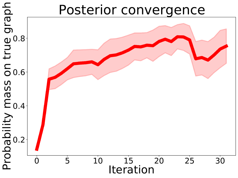
(a)

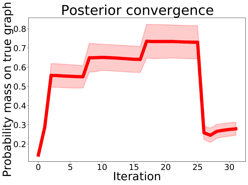
(b)

Figure 5: Evolution of $P(G=\mathcal{G})$ across iterations in the experiment using the synthetic graph. (a) is the posterior as given by cd-cbo, whereas (b) is that given by ceo. As discussed in Section 5, we found this an interesting example where the true graph is hard to distinguish from an alternative one, but causal optimization can still proceed efficiently. Note that in both healthcare and epidemiology examples we found the graph to be identified easily by our posterior.

Appendix E Further discussion on Causal Entropy Search and related literature

Compared to acquisition functions in prior related works [2, 67, 59], several important challenges arise specific to our goals as specified by Eq. 1: to start with, the acquisition used in cbo cannot be straightforwardly extended to our setting. Firstly, because it is not clear how to incorporate our graph prior in a principled manner. Secondly, as explained in Section 3.1, we cannot assume that we can observe the causal effect exactly, since observations from the sem are noisy, and the family of expected-improvement (ei) acquisitions are known to be inappropriate in this setting [17, 20]. We addressed these challenges by introducing an information-theoretic acquisition function. These types of objectives are widely used in boed [13], active learning [40] as well as many bo approaches [29, 67, 45]. The information-theoretic approach is often advocated in bo because, contrasted to approaches like ei that largely judge optimization performance based solely on having found high objective function values, it seeks data that is maximally informative about a variable of interest [20]. In practice, these approaches can be better suited to challenging noisy problems, multimodal and non-smooth functions, or optimization with multiple information sources [17]. It is worth keeping in mind that there is no uniformly best acquisition across all settings.

Output space vs input space ES We decided to frame causal optimization as learning about $y^{\star}$ rather than $\mathbf{x}^{\star}$. The question of whether to perform output-space ES (what we do) versus input-space ES has been studied before in bo; see [20, §6] and [45]. However, a crucial difficulty is added in causal optimization: there are multiple surrogate models, each with different input space and dimensionality; one for each intervention set $\mathbf{X}_{I}\in\textsc{{es}}$ we want to consider. Having multiple surrogates is similar to the setting of multi-task bo [59]; however (1) our tasks do not share input space and (2) we do not know which task actually contains the global optimum. Therefore, while in principle learning about $\mathbf{x}^{\star}$ could be done, it would be computationally expensive and inference-wise challenging to define a distribution over a variable with varying (and potentially large) dimensionality. On the other hand, all causal effects share $Y$, which is one dimensional. Future work could consider inference techniques for dimension-varying parameters like reversible-jump mcmc [23].

Appendix F Further discussion on surrogate models

A surrogate model for each graph?

Notice that one can think of a very different way to incorporate uncertainty: we could define distinct surrogate models for each $g$ in the support $R_{G}$ of $P(G)$. We do not take this approach for several reasons: (1) it would not extend to a setting where we need to approximate expectations under $P(G)$ with sampling (hence it is not scalable in this sense); (2) it would require $|R_{G}|\cdot|\textsc{{es}}|$ kernel hyperparameters to store and update at every iteration; (3) finally, modelling the true causal effect by marginalizing the graph in this approach would lead to a weighted mixture of gps, rendering inference and bo complicated.

Appendix G Further derivations

The variance term in Eq. 4 is computed as

$$\mathbb{V}[\hat{\mathbb{E}}{\left[Y\mid\text{do}(\mathbf{X}_{I}=\mathbf{x}_{I}),G\right]}]=\mathbb{E}{\left[\left[\widehat{\mathbb{E}}[Y|\text{do}(\mathbf{X}_{I}=\mathbf{x}_{I}),G]\right]^{2}\right]}-(m_{I}(\mathbf{x}_{I}))^{2}.$$ (14)

Appendix H Belief over the optimal set

We compute $P(\mathbf{X}_{I}=\mathbf{X}_{I}^{\star})$ as:

$$P(\mathbf{X}_{I}=\mathbf{X}_{I}^{\star})=\frac{e^{\mu_{I}^{\star}+\beta\cdot\sigma_{I}^{\star}}}{\sum_{I^{\prime}}e^{\mu_{I^{\prime}}^{\star}+\beta\cdot\sigma_{I^{\prime}}^{\star}}}$$ (15)

when maximizing a causal effect, with signs reversed when minimizing. Here, $\mu_{I}^{\star}$ is the minimum of the mean function of surrogate model $f_{I}$, and $\sigma_{I}^{\star}$ the standard deviation of the univariate Gaussian with mean at that point. We did not explore adaptive tuning of $\beta$ which we fixed to $0.1$. Guarantees for UCB can be found in e.g. [20].

H.1 Parametric assumptions

Firstly, the additive Gaussian noise assumption (let us call it AGN- additive Gaussian noise) combined with GPs on the structural equations allows us to define the graph likelihood in closed form. This also implies that GP posteriors on the structural functions are available in closed form. When AGN does not hold, one would need to resort to the literature on Variational GPs, which allows one to perform inference with GPs with non-Gaussian likelihoods. Secondly, the AGN assumption also allows us to deal with noisy Bayesian optimization [20]. Recall that, even if we knew the graph, we do not get to observe $\mathbb{E}[Y\mid\text{do}({\mathbf{X}_{I}}={\mathbf{x}_{I}}),G]$, but can only get samples from $p(Y\mid\text{do}({\mathbf{X}_{I}}={\mathbf{x}_{I}}),G)$. BO with non-Gaussian noise is an active area of research, see e.g. [16] who allow for sub-Gaussian likelihood noises. The optimization becomes more sophisticated, and note that CEO (and CBO) needs to deal with multiple surrogate models (one for each $\mathbf{X}_{I}$). Therefore, extending these methods from the BO setting to CBO and CEO is a future area of research.
Finally, beyond the previously discussed additive Gaussian noise assumption, in our experiments we used radial basis function kernels, consistently with previous works on CBO. These were appropriate kernels for the SCMs we studied in the experiments; however, for nonstationary causal effect functions one could use nonstationary GP kernels.

Appendix I Synthetic: graphs and true sem

For the sem of the synthetic graph, see the Supplementary material of [2]. For all experiments, we used standard radial basis function (RBF) kernels, and optimized hyperparameters with type $II$ maximum likelihood.

(a)

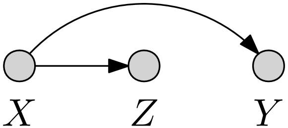
(b)

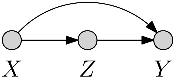
(c)

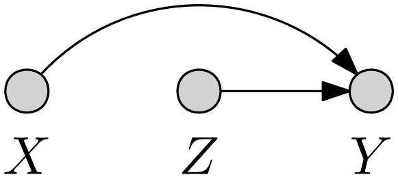
(d)

(e)

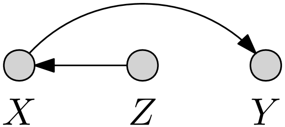
(f)

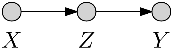
(g)

Figure 6: Graph prior $P(G)$ used for the synthetic experiment s.t. $|R_{G}|=6$. The true dag is shown in Fig. 6(g).

Appendix J Epidemiology: graphs and true sem

We use a modified (more challenging and nonliner) version of the sem only partially specified in [28]:

$$B =\mathcal{U}[-1,1]$$ (16)

$$T =\mathcal{U}[4,8]$$ (17)

$$L =\text{expit}(0.5\cdot T+U)$$ (18)

$$R =4+L\cdot T$$ (19)

$$Y =0.5+\cos(4\cdot T)+\sin(-L+2\cdot R)+U+\epsilon\qquad\text{with}\leavevmode\nobreak\ \leavevmode\nobreak\ \epsilon\leavevmode\nobreak\ \leavevmode\nobreak\ \sim\mathcal{N}(0,1)$$ (20)

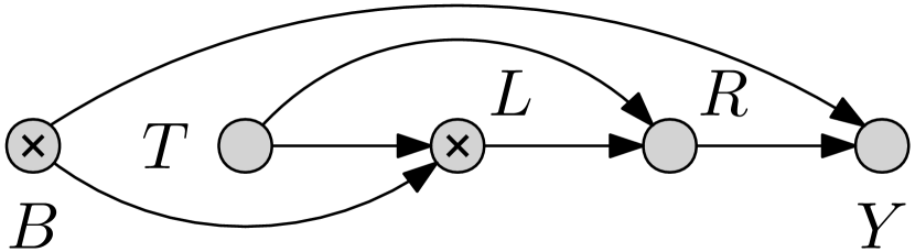
(a)

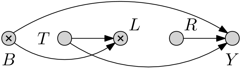
(b)

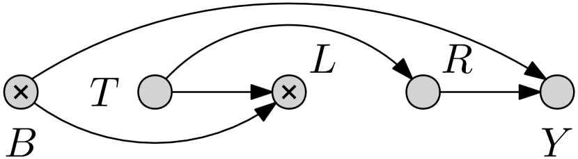
(c)

(d)

Figure 7: Graph prior $P(G)$ used for the epidemiology experiment s.t. $|R_{G}|=3$. The true dag is shown in Fig. 7(d).

Appendix K Healthcare: : graphs and true sem

For the sem see the Supplementary material of [2]. In this example, we had initial points $|\mathcal{D}^{{I}}|=2$.

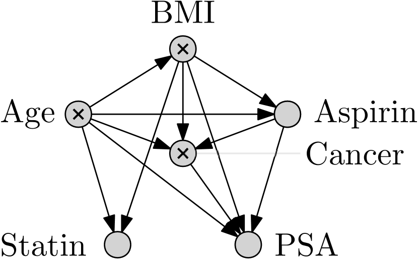
(a)

(b)

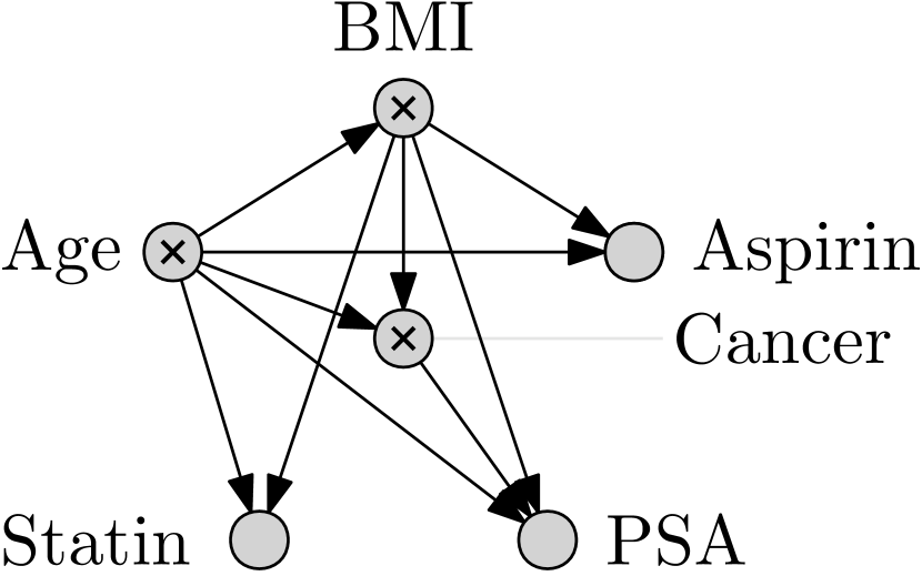
(c)

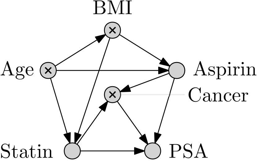
(d)

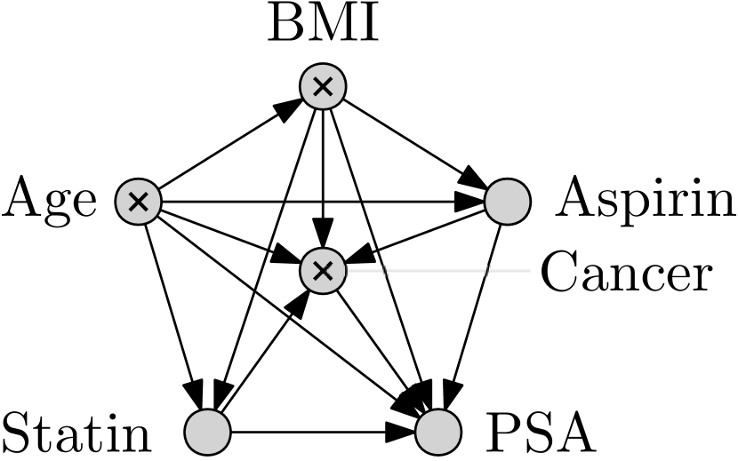
(e)

Figure 8: Graph prior $P(G)$ used for the health experiment s.t. $|R_{G}|=4$. The true dag is shown in Fig. 8(e).

Appendix L Entropy in Causality

There is a large literature on the use of information theoretic concepts with applications to causal inference, discovery and counterfactual reasoning. The information-geometric approach to causal discovery [32] attempts to lift the strict conditional independence requirement of classical algorithms like PC [57], by defining independence as orthogonality in information space. They find that in important examples this induces a desirable asymmetry between cause and effect. Miklin et al. [44] find use in entropies between variables of a causal Bayesian network in deriving so-called causal inequalities, which are bounds on certain quantities that characterize the behaviour of the underlying system represented by the CBN. Recently, Kocaoglu et al. [34] introduced a framework, “Entropic Causal Inference”, where the causal direction between two categorical variable can be discerned from observational data based on an interesting condition on the entropy of the exogenous variable.

Appendix M Computational Complexity

We provide here more details on computational complexity.
We have now added a paragraph in Section 3.3 about complexity and a new Section in the Supplement with more details The complexity of CEO is driven by the computation of CES. The parameters influencing these are: $|\mathbf{ES}|$, $\max_{I}|\mathbf{X}_{I}|$, the number of acquisition points $N$ (i.e., how many values of the intervened variable to consider, assuming the same number for all $\mathbf{X}_{I}$). Therefore, the total complexity of the acquisition is $\mathcal{O}(N\cdot\text{CES}(\mathbf{x})\cdot\sum_{\mathbf{X}_{I}\in\mathbf{ES}}|\mathbf{X}_{I}|)$. Here, $\text{CES}(\mathbf{x})$ denotes the time needed to compute CES for m specific value $\mathbf{x}$, regardless of its corresponding $\mathbf{X}_{I}$. Note this is valid for CBO also, replacing $\text{CES}(\mathbf{x})$ with $\text{CEI}(\mathbf{x})$, the acquisition used by CBO. However,$\text{CEI}(\mathbf{x})$ is cheaper than $\text{CES}(\mathbf{x})$. The biggest reason in practice is that CEI operations can be more easily vectorized. CES operations however can be parallelized over both $\mathbf{ES}$ and values of $\mathbf{x}_{I}$. Our implementation indeed uses KDEs, but it does so only to estimate univariate marginal distributions, which is not very expensive (no curse of dimensionality). Graph sizes: Since in our setting the number of nodes is not too large, there is a tractable number of graphs that can be enumerated, therefore omitted in the above Big-O notation. As mentioned in Appendix B, larger spaces of graphs could be explored in future work by sampling with MCMC as common in the structure learning literature, losing however our closed form expectations over the graph. Work that explores the full space of DAGs with many nodes will necessarily introduce additional approximations. We also discussed scalability in the limitations in Section 6. It is a general limitation, not restricted to CEO, that in causal global optimization problems one needs to train $|\mathbf{ES}|$ GPs ( in general $|\mathbf{ES}|$ will scale as $2^{|\mathbf{X}|}$), which does not scale with large graphs (here exact GP inference is cubic in the number of collected interventions).

Appendix N Further experimental details and additional results

We provide here additional experimental results. In Table 3 and Fig. 9 we show that, as in our previous experiment, CD-CBO performs worse than ceo, and in this case slightly better than CBO on the true graph. Since as we mentioned in Section 5, in this example we initially found that our acquisition finds the graph too fast (i.e., at initialization), and therefore it would not be possible to compare to CD-CBO, to provide this additional comparison we updated all graph posteriors (of all methods) only with interventions and not with observational data. This only amplifies the signal between the difference among CD-CBO and CBO, and has no other side-effects on the performance comparison; note that if the graph is found immediately, then CD-CBO is CBO.

Table 3: Average gap $\pm$ one standard error computed across 12 replicates initialized with different $\mathcal{D}$. Higher values are better, and $0\leq$ gap $\leq 1$. The best result for each experiment in bold.

Method	Synthetic	Epidemiology (Fig. 4)
ceo	0.75 $\pm 0.03$	$0.58\pm 0.05$
cbo w. $G=\mathcal{G}$	$0.66\pm 0.04$	0.62$\pm 0.02$
cbo w. $G\neq\mathcal{G}$	$0.59\pm 0.035$	$0.46\pm 0.05$
$\textsc{cd}-\textsc{cbo}$	$0.39\pm 0.04$	$0.52\pm 0.04$

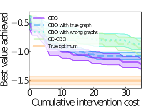
Figure 9: Additional results for a comparision with CD-CBO on the Epidemiology example.

References

- Aglietti et al. [2020a] V. Aglietti, T. Damoulas, M. Álvarez, and J. González. Multi-task causal learning with gaussian processes. In Advances in Neural Information Processing Systems, volume 33, 2020a.
- Aglietti et al. [2020b] V. Aglietti, X. Lu, A. Paleyes, and J. González. Causal bayesian optimization. In International Conference on Artificial Intelligence and Statistics, pages 3155–3164. PMLR, 2020b.
- Aglietti et al. [2021] V. Aglietti, N. Dhir, J. González, and T. Damoulas. Dynamic causal bayesian optimization. Advances in Neural Information Processing Systems, 34, 2021.
- Agrawal et al. [2019] R. Agrawal, C. Squires, K. Yang, K. Shanmugam, and C. Uhler. Abcd-strategy: Budgeted experimental design for targeted causal structure discovery. In K. Chaudhuri and M. Sugiyama, editors, Proceedings of Machine Learning Research, volume 89 of Proceedings of Machine Learning Research, pages 3400–3409. PMLR, 16–18 Apr 2019.
- Andersson et al. [1997] S. A. Andersson, D. Madigan, M. D. Perlman, et al. A characterization of markov equivalence classes for acyclic digraphs. Annals of statistics, 25(2):505–541, 1997.
- Angrist and Imbens [1995] J. Angrist and G. Imbens. Identification and estimation of local average treatment effects, 1995.
- Atan et al. [2018] O. Atan, J. Jordon, and M. van der Schaar. Deep-treat: Learning optimal personalized treatments from observational data using neural networks. In Proceedings of the AAAI Conference on Artificial Intelligence, volume 32, 2018.
- Chickering [1996] D. M. Chickering. Learning bayesian networks is np-complete. In Learning from data, pages 121–130. Springer, 1996.
- Chickering [2002] D. M. Chickering. Optimal structure identification with greedy search. Journal of machine learning research, 3(Nov):507–554, 2002.
- Compton et al. [2022] S. Compton, K. Greenewald, D. A. Katz, and M. Kocaoglu. Entropic causal inference: Graph identifiability. In International Conference on Machine Learning, pages 4311–4343. PMLR, 2022.
- Cooper and Yoo [1999] G. F. Cooper and C. Yoo. Causal discovery from a mixture of experimental and observational data. In Proceedings of the Fifteenth Conference on Uncertainty in Artificial Intelligence, UAI’99, page 116–125, San Francisco, CA, USA, 1999. Morgan Kaufmann Publishers Inc. ISBN 1558606149.
- Cover [1999] T. M. Cover. Elements of information theory. John Wiley & Sons, 1999.
- Drovandi et al. [2017] C. C. Drovandi, C. Holmes, J. M. McGree, K. Mengersen, S. Richardson, and E. G. Ryan. Principles of experimental design for big data analysis. Statistical science: a review journal of the Institute of Mathematical Statistics, 32(3):385, 2017.
- Eaton and Murphy [2007a] D. Eaton and K. Murphy. Bayesian structure learning using dynamic programming and mcmc. Uncertainty in Artificial Intelligence, 2007a.
- Eaton and Murphy [2007b] D. Eaton and K. Murphy. Exact bayesian structure learning from uncertain interventions. In Artificial intelligence and statistics, pages 107–114. PMLR, 2007b.
- Faria et al. [2022] G. R. A. Faria, A. Martins, and M. A. Figueiredo. Differentiable causal discovery under latent interventions. In Conference on Causal Learning and Reasoning, pages 253–274. PMLR, 2022.
- Frazier [2018] P. I. Frazier. Bayesian optimization. In Recent Advances in Optimization and Modeling of Contemporary Problems, pages 255–278. INFORMS, 2018.
- Friedman and Koller [2003] N. Friedman and D. Koller. Being Bayesian about network structure; a Bayesian approach to structure discovery in Bayesian networks. Machine learning, 50(1):95–125, 2003.
- Gamella and Heinze-Deml [2020] J. L. Gamella and C. Heinze-Deml. Active invariant causal prediction: Experiment selection through stability. arXiv preprint arXiv:2006.05690, 2020.
- Garnett [2022] R. Garnett. Bayesian Optimization. Cambridge University Press, 2022. in preparation.
- Ghassami et al. [2018] A. Ghassami, S. Salehkaleybar, N. Kiyavash, and E. Bareinboim. Budgeted experiment design for causal structure learning. In International Conference on Machine Learning, pages 1724–1733. PMLR, 2018.
- Glymour et al. [2019] C. Glymour, K. Zhang, and P. Spirtes. Review of causal discovery methods based on graphical models. Frontiers in genetics, 10:524, 2019.
- Green [1995] P. J. Green. Reversible jump markov chain monte carlo computation and bayesian model determination. Biometrika, 82(4):711–732, 1995.
- Håkansson et al. [2020] S. Håkansson, V. Lindblom, O. Gottesman, and F. D. Johansson. Learning to search efficiently for causally near-optimal treatments. arXiv preprint arXiv:2007.00973, 2020.
- Hauser and Bühlmann [2012] A. Hauser and P. Bühlmann. Characterization and greedy learning of interventional markov equivalence classes of directed acyclic graphs. The Journal of Machine Learning Research, 13(1):2409–2464, 2012.
- Hauser and Bühlmann [2014] A. Hauser and P. Bühlmann. Two optimal strategies for active learning of causal models from interventional data. International Journal of Approximate Reasoning, 55(4):926–939, 2014.
- Hauser and Bühlmann [2015] A. Hauser and P. Bühlmann. Jointly interventional and observational data: estimation of interventional markov equivalence classes of directed acyclic graphs. Journal of the Royal Statistical Society: Series B (Statistical Methodology), 77(1):291–318, 2015.
- Havercroft and Didelez [2012] W. Havercroft and V. Didelez. Simulating from marginal structural models with time-dependent confounding. Statistics in medicine, 31(30):4190–4206, 2012.
- Hennig and Schuler [2012] P. Hennig and C. J. Schuler. Entropy search for information-efficient global optimization. Journal of Machine Learning Research, 13(6), 2012.
- Horii [2021] S. Horii. Bayesian model averaging for causality estimation and its approximation based on gaussian scale mixture distributions. In International Conference on Artificial Intelligence and Statistics, pages 955–963. PMLR, 2021.
- Hyttinen et al. [2015] A. Hyttinen, F. Eberhardt, and M. Järvisalo. Do-calculus when the true graph is unknown. In UAI, pages 395–404. Citeseer, 2015.
- Janzing et al. [2012] D. Janzing, J. Mooij, K. Zhang, J. Lemeire, J. Zscheischler, P. Daniušis, B. Steudel, and B. Schölkopf. Information-geometric approach to inferring causal directions. Artificial Intelligence, 182:1–31, 2012.
- Kocaoglu et al. [2017a] M. Kocaoglu, A. Dimakis, and S. Vishwanath. Cost-optimal learning of causal graphs. In International Conference on Machine Learning, pages 1875–1884. PMLR, 2017a.
- Kocaoglu et al. [2017b] M. Kocaoglu, A. G. Dimakis, S. Vishwanath, and B. Hassibi. Entropic causal inference. In Thirty-First AAAI Conference on Artificial Intelligence, 2017b.
- Kocaoglu et al. [2020] M. Kocaoglu, S. Shakkottai, A. G. Dimakis, C. Caramanis, and S. Vishwanath. Applications of common entropy for causal inference. Advances in neural information processing systems, 33:17514–17525, 2020.
- Kuipers and Moffa [2017] J. Kuipers and G. Moffa. Partition mcmc for inference on acyclic digraphs. Journal of the American Statistical Association, 112(517):282–299, 2017.
- Lattimore et al. [2016] F. Lattimore, T. Lattimore, and M. D. Reid. Causal bandits: Learning good interventions via causal inference. arXiv preprint arXiv:1606.03203, 2016.
- Lattimore and Szepesvári [2020] T. Lattimore and C. Szepesvári. Bandit algorithms. Cambridge University Press, 2020.
- Lu et al. [2021] Y. Lu, A. Meisami, and A. Tewari. Causal bandits with unknown graph structure. Advances in Neural Information Processing Systems, 34, 2021.
- MacKay [1992] D. J. MacKay. Information-based objective functions for active data selection. Neural computation, 4(4):590–604, 1992.
- Madigan et al. [1995] D. Madigan, J. York, and D. Allard. Bayesian graphical models for discrete data. International Statistical Review/Revue Internationale de Statistique, pages 215–232, 1995.
- Marx et al. [2021] A. Marx, L. Yang, and M. van Leeuwen. Estimating conditional mutual information for discrete-continuous mixtures using multi-dimensional adaptive histograms. In Proceedings of the 2021 SIAM International Conference on Data Mining (SDM), pages 387–395. SIAM, 2021.
- Masegosa and Moral [2013] A. R. Masegosa and S. Moral. An interactive approach for bayesian network learning using domain/expert knowledge. International Journal of Approximate Reasoning, 54(8):1168–1181, 2013.
- Miklin et al. [2017] N. Miklin, A. A. Abbott, C. Branciard, R. Chaves, and C. Budroni. The entropic approach to causal correlations. New Journal of Physics, 19(11):113041, 2017.
- Moss [2021] H. Moss. General-purpose Information-theoretical Bayesian Optimisation: A thesis by acronyms. PhD thesis, Lancaster University, 2021.
- Murphy [2001] K. P. Murphy. Active learning of causal bayes net structure. Technical report, 2001.
- Ness et al. [2017] R. O. Ness, K. Sachs, P. Mallick, and O. Vitek. A bayesian active learning experimental design for inferring signaling networks. In International Conference on Research in Computational Molecular Biology, pages 134–156. Springer, 2017.
- Owen [2013] A. B. Owen. Monte Carlo theory, methods and examples. 2013.
- Pearl [2009] J. Pearl. Causality. Cambridge university press, 2009.
- Peters et al. [2017] J. Peters, D. Janzing, and B. Schölkopf. Elements of causal inference: foundations and learning algorithms. The MIT Press, 2017.
- Rosenbaum and Rubin [1983] P. R. Rosenbaum and D. B. Rubin. The central role of the propensity score in observational studies for causal effects. Biometrika, 70(1):41–55, 1983.
- Sgouritsa [2015] E. Sgouritsa. Causal Discovery Beyond Conditional Independencies. PhD thesis, University of Tubingen, 2015.
- Shimizu et al. [2006] S. Shimizu, P. O. Hoyer, A. Hyvärinen, A. Kerminen, and M. Jordan. A linear non-gaussian acyclic model for causal discovery. Journal of Machine Learning Research, 7(10), 2006.
- Silva [2016] R. Silva. Observational-interventional priors for dose-response learning. arXiv preprint arXiv:1605.01573, 2016.
- Silva and Gramacy [2010] R. Silva and R. B. Gramacy. Gaussian process structural equation models with latent variables. arXiv preprint arXiv:1002.4802, 2010.
- Spirtes et al. [2000a] P. Spirtes, C. Glymour, R. Scheines, S. Kauffman, V. Aimale, and F. Wimberly. Constructing bayesian network models of gene expression networks from microarray data. 2000a.
- Spirtes et al. [2000b] P. Spirtes, C. N. Glymour, R. Scheines, and D. Heckerman. Causation, prediction, and search. MIT press, 2000b.
- Steudel and Ay [2015] B. Steudel and N. Ay. Information-theoretic inference of common ancestors. Entropy, 17(4):2304–2327, 2015.
- Swersky et al. [2013] K. Swersky, J. Snoek, and R. P. Adams. Multi-task bayesian optimization. In C. J. C. Burges, L. Bottou, M. Welling, Z. Ghahramani, and K. Q. Weinberger, editors, Advances in Neural Information Processing Systems, volume 26. Curran Associates, Inc., 2013.
- Tong and Koller [2001] S. Tong and D. Koller. Active learning for structure in bayesian networks. In International joint conference on artificial intelligence, volume 17, pages 863–869. Citeseer, 2001.
- Verma and Pearl [1991] T. Verma and J. Pearl. Equivalence and synthesis of causal models. UCLA, Computer Science Department, 1991.
- Viinikka and Koivisto [2020] J. Viinikka and M. Koivisto. Layering-mcmc for structure learning in bayesian networks. In J. Peters and D. Sontag, editors, Proceedings of the 36th Conference on Uncertainty in Artificial Intelligence (UAI), volume 124 of Proceedings of Machine Learning Research, pages 839–848. PMLR, 03–06 Aug 2020.
- von Kügelgen et al. [2019] J. von Kügelgen, P. K. Rubenstein, B. Schölkopf, and A. Weller. Optimal experimental design via bayesian optimization: active causal structure learning for gaussian process networks. In NeurIPS 2019 Workshop Do the right thing: machine learning and causal inference for improved decision making. NeurIPS, Dec. 2019.
- Vowels et al. [2021] M. J. Vowels, N. C. Camgoz, and R. Bowden. D’ya like dags? a survey on structure learning and causal discovery. arXiv preprint arXiv:2103.02582, 2021.
- Wang and Zhou [2021] T.-Z. Wang and Z.-H. Zhou. Actively identifying causal effects with latent variables given only response variable observable. Advances in Neural Information Processing Systems, 34, 2021.
- Wang et al. [2017] Y. Wang, L. Solus, K. D. Yang, and C. Uhler. Permutation-based causal inference algorithms with interventions. arXiv preprint arXiv:1705.10220, 2017.
- Wang and Jegelka [2017] Z. Wang and S. Jegelka. Max-value entropy search for efficient bayesian optimization. In International Conference on Machine Learning, pages 3627–3635. PMLR, 2017.
- Williams and Rasmussen [2006] C. K. Williams and C. E. Rasmussen. Gaussian processes for machine learning, volume 2. MIT press Cambridge, MA, 2006.
- Wilson et al. [2018] J. Wilson, F. Hutter, and M. Deisenroth. Maximizing acquisition functions for bayesian optimization. Advances in neural information processing systems, 31, 2018.
- Yang et al. [2018] K. Yang, A. Katcoff, and C. Uhler. Characterizing and learning equivalence classes of causal dags under interventions. In International Conference on Machine Learning, pages 5541–5550. PMLR, 2018.
- Zemplenyi and Miller [2021] M. Zemplenyi and J. W. Miller. Bayesian optimal experimental design for inferring causal structure. arXiv preprint arXiv:2103.15229, 2021.
- Zhang et al. [2012] B. Zhang, A. A. Tsiatis, E. B. Laber, and M. Davidian. A robust method for estimating optimal treatment regimes. Biometrics, 68(4):1010–1018, 2012.
- Zhang [2020] J. Zhang. Designing optimal dynamic treatment regimes: A causal reinforcement learning approach. In International Conference on Machine Learning, pages 11012–11022. PMLR, 2020.
- Zhang et al. [2015] K. Zhang, Z. Wang, J. Zhang, and B. Schölkopf. On estimation of functional causal models: general results and application to the post-nonlinear causal model. ACM Transactions on Intelligent Systems and Technology (TIST), 7(2):1–22, 2015.