What Quantum Strings can tell us about
Quantum Gravity

Abstract

I describe the recent progress in resolving two problems of nonperturbative bosonic string inherited from 1980’s. Both the lattice and KPZ-DDK no-go theorems can be bypassed thanks to specific features of the theory with diffeomorphism invariance.

Institute of Theoretical and Experimental Physics, Moscow E-mail: makeenko@itep.ru

PACS: 11.25.Pm, 11.15.Pg

1 Introduction

This Talk is based on the recent papers [2, 1] written partially in collaboration with Jan Ambjørn. Accurate references to the cited results of other authors can be found there. While the papers are relatively new, the problems they are devoted are inherited from 1980’s and were formulated as two no-go theorems for string existence.

1) The non-perturbative regularization of the Nambu-Goto string by a hypercubic lattice does not scale to a continuum string for the embedding space dimension $d\geq 2$ as found by Durhuus, Fröhlich, Jonsson (1984). Analogously the regularization of the Polyakov string by dynamical triangulation scales to continuum only for $d\leq 1$ but does not for $d>1$ as shown by Ambjørn, Durhuus (1987).

2) The string susceptibility index of (closed) Polyakov’s string, calculated by Knizhnik-Polyakov-Zamolodchikov (1988), David (1988), Distler-Kawai (1989) using the conformal theory technique, is not real for $1<d<25$

$$\gamma_{\rm str}=(1-{h})\frac{d-25-\sqrt{(d-1)(d-25)}}{12}+2\qquad\framebox{{genus} $h$}$$

The possible solutions of these two problems are described in my talk and rely on subtleties in quantum field theory enjoying diffeomorphism invariance like Strings(!) and Gravity(?):

1) The continuum limit is not as in usual quantum field theory: the Lilliputian scaling regime versus an infinite correlation length.

2) The Nambu-Goto and Polyakov strings are told apart by higher derivative terms in the emergent action which are classically suppressed with the UV cuttoff $\Lambda\to\infty$ as $\sim\Lambda^{-2}$ but revive quantumly as $\Lambda^{-2}\times\Lambda^{2}\sim 1$.

2 Mean-field ground state of bosonic string

The action of the Polyakov string is quadratic in the target-space coordinate $X^{\mu}$ and has an independent metric tensor $\rho_{ab}$. The Nambu-Goto string can also be written like it by introducing the Lagrange multiplier $\lambda^{ab}$. The two string formulations are expected to be equivalent as shown classically by Polyakov (1981) and at one loop by Fradkin, Tseytlin (1982). The general argument is given in the book by Polyakov (1987).

We consider a closed bosonic string winding once around compactified dimension of circumference $\beta$ and propagating through an (Euclidean) time $L$ (topology of a cylinder or a torus). There are no tachyonic states if $\beta$ is large enough. Choosing the world-sheet parameters $\omega_{1},\omega_{2}\in\omega_{L}\times\omega_{\beta}$ inside a rectangle, the classical ground state $X^{\mu}_{\rm cl}$ and $\rho^{ab}_{\rm cl}$ is usual and $\lambda^{ab}_{\rm cl}=\rho^{ab}_{\rm cl}\sqrt{\rho_{\rm cl}}$ simplifies to $\lambda^{ab}_{\rm cl}=\delta^{ab}$ in the conformal gauge $\rho_{ab}=\rho\delta_{ab}$ for $\omega_{L}/\omega_{\beta}=L/\beta$.

Let us do the Gaussian path integral over $X^{\mu}_{\rm q}$ by splitting $X^{\mu}=X^{\mu}_{\rm cl}+X^{\mu}_{\rm q}$:

$$S_{\rm ind}=K_{0}\int{\rm d}^{2}\omega\,\sqrt{\rho}+\frac{K_{0}}{2}\int{\rm d}^{2}\omega\,\lambda^{ab}\left(\partial_{a}X_{\rm cl}\cdot\partial_{b}X_{\rm cl}-\rho_{ab}\right)+\frac{d}{2}{\rm tr}\,\log{\cal O},$$

where the operator ${\cal O}=-\frac{1}{\sqrt{\rho}}\partial_{a}\lambda^{ab}\partial_{b}$ reproduces the Laplacian $\Delta$ for $\lambda^{ab}=\rho^{ab}\sqrt{\det\rho}$. An additional ghost determinant also emerges as usual in the conformal gauge. The action is called induced (or emergent). It coincides with the effective action for smooth fields.

Two-dimensional determinants diverge and have to be regularized. For Schwinger’s proper-time regularization the integrals over $\tau$ are simply cut from below at $a^{2}=1/4\pi\Lambda^{2}$. We use instead Pauli-Villars’ regularization by Ambjørn, Y.M. (2017)

$$\det({\cal O})\big{|}_{\rm reg}\equiv\frac{\det({\cal O})\det({\cal O}+2M^{2})}{\det({\cal O}+M^{2})^{2}}$$

when

$${\rm tr}\,\log{\cal O}\big{|}_{\rm reg}=-\int_{0}^{\infty}\frac{{\rm d}\tau}{\tau}\,{\rm tr}\,{\,\rm e}^{-\tau{\cal O}}\left(1-{\,\rm e}^{-\tau M^{2}}\right)^{2},\quad~{}~{}\Lambda^{2}=\frac{M^{2}}{2\pi}\log 2$$

is convergent at finite regulator mass $M$ and divergent as $M\to\infty$.

For Pauli-Villars’ regularization a beautiful diagrammatic technique applies and the det’s can be exactly computed for certain metrics by the Gel’fand-Yaglom technique to compare with the Seeley expansion which starts with the term $1/\tau$ in two dimensions. For $\tau\sim 1/\Lambda^{2}$ the higher terms are suppressed as $R/\Lambda^{2}$ for smooth fields but revive if they are not.

It is easy to compute the effective action $S_{\rm eff}$ for diagonal and constant $\lambda^{ab}=\bar{\lambda}\delta^{ab}$ and $\rho_{ab}=\bar{\rho}\delta_{ab}$. Omitting the boundary terms for $L\gg\beta$, the minimum of $S_{\rm eff}$ is reached at the quantum ground state

$$\bar{\lambda}=\frac{1}{2}\left(1+\frac{\Lambda^{2}}{K_{0}}+\sqrt{\left(1+\frac{\Lambda^{2}}{K_{0}}\right)^{2}-\frac{2d\Lambda^{2}}{K_{0}}}\right),\qquad\bar{\rho}\propto\frac{{\bar{\lambda}}}{\sqrt{\Big{(}1+\frac{\Lambda^{2}}{K_{0}}\Big{)}^{2}-\frac{2d\Lambda^{2}}{K_{0}}}}$$

as found by Ambjørn, Y.M. (2017). The minimization over $\omega_{\beta}/\omega_{L}$ is also needed at the saddle point.

The approximation describes a mean field which takes into account an infinite set of pertubative diagrams about the classical vacuum. Then $\lambda^{ab}$ and $\rho_{ab}$ do not fluctuate in the mean-field approximation which becomes exact at large $d$.

It is like the two-dimensional $O(N)$ sigma model at large $N$, where the Lagrange multiplier does not fluctuate (summing the bubble graphs). The large-$N$ vacuum is very close to the physical vacuum even for $N=3$.

The square root in $\bar{\lambda}$ and $\bar{\rho}$ is well-defined for ${d\geq 2}$ if

$$K_{0}>K_{*}=\left(d-1+\sqrt{d^{2}-2d}\right)\Lambda^{2}\stackrel{{\scriptstyle d\to\infty}}{{\to}}2d\Lambda^{2}$$

The perturbation theory is recovered by expanding in $1/K_{0}\sim\hbar$. Then ${\bar{\lambda}}$ ranges between 1 (the classical value) and the (quantum) value

$${\bar{\lambda}}_{*}=\frac{1}{2}\left(d-\sqrt{d^{2}-2d}\right)\stackrel{{\scriptstyle d\to\infty}}{{\to}}\frac{1}{2}$$

A natural question is as to why the minimum of the action is reached at constant $\bar{\rho}$ and $\bar{\lambda}$. I shall confirm it in Sect. 5 by showing a stability of this ground state under fluctuations.

3 Two scaling regimes: Gulliver’s vs. Lilliputian

The mean-field ground state energy is like found by Alvarez (1981), Arvis (1983)

$$E_{N}(\beta)=K_{0}{\bar{\lambda}}\sqrt{\beta^{2}+\frac{1}{K_{0}{\bar{\lambda}}}\left(-\frac{\pi(d-2)}{3}+8N\right)}$$

and does not scale because $K_{0}>K_{*}\sim\Lambda^{2}$ for ${\bar{\lambda}}$ to be real ($>{\bar{\lambda}}_{*}$). Let us choose $\beta^{2}$ slightly larger $\beta^{2}_{\rm min}=\frac{\pi(d-2)}{3K_{*}{\bar{\lambda}}_{*}}$ for not to have a tachyon. It is clear that the ground-state energy $E_{0}(\beta)$ can be made finite by fine tuning $\beta$.

This scaling does not exist for excited states and thus is particle-like similar to the lattice regularizations of a string, where only the lowest mass scales to finite while excitations scale to infinity, reproducing the results by Durhuus, Fröhlich, Jonsson (1984), Ambjørn, Durhuus (1987).

Let us ‘‘renormalize’’ the units of length

$$L_{R}=\sqrt{\frac{{\bar{\lambda}}}{{\bar{\lambda}}-{\bar{\lambda}}_{*}}}\,L,\qquad\beta_{R}=\sqrt{\frac{{\bar{\lambda}}}{{\bar{\lambda}}-{\bar{\lambda}}_{*}}}\,\beta$$

to obtain a finite effective action

$$S_{\rm mf}=K_{R}\;L_{R}\sqrt{\beta_{R}^{2}-\frac{\pi(d-2)}{3K_{R}}},\qquad K_{R}=K_{0}({\bar{\lambda}}-{\bar{\lambda}}_{*})$$

The renormalized string tension $K_{R}$ scales to finite if $K_{0}\to K_{*}$ reproducing the Alvarez-Arvis spectrum of the continuum string. The average area is also finite recovering the minimal area for large $\beta_{R}$.

The Lilliputian scaling regime is analogous to the zeta-function regularization except for the nonlinearities, but the bare length in target space is of order of the cutoff. This is why it was called Lilliputian. Such a scaling exists because $\bar{\rho}\to\infty$ as $K_{0}\to K_{*}$.

For this reason the cutoff in parameter space is $\Delta\omega=1/(\Lambda\sqrt[4]{g})$ which fixes the maximal number of modes in the mode expansion to be $n_{\rm max}\sim\Lambda\sqrt[4]{g}\omega_{\beta}$. Classically $\sqrt[4]{g}\omega_{\beta}=\beta$ but quantumly $\sqrt[4]{g}\omega_{\beta}\propto\frac{\sqrt{K_{0}}\,\beta}{\sqrt{K_{R}}}$ is much larger.

The Lilliputian scaling describes continuum because infinitely smaller distances can be probed $\Longrightarrow$ classical music can be played on the Lilliputian strings. Gulliver’s tools are too coarse to resolve the Lilliputian world. This is why the lattice string regularizations of 1980’s never reproduce canonical quantization.

4 Instability of the classical ground state

The semiclassical (or one-loop) correction due to zero-point fluctuations was first computed by Brink, Nielsen (1973)

$$S_{1l}=\left[K_{0}-\frac{(d-2)}{2}\Lambda^{2}\right]L\beta-\frac{\pi(d-2)L}{6\beta}$$

To make it finite, it is custom to introduce the renormalized string tension

$$K_{R}=K_{0}-\frac{(d-2)}{2}\Lambda^{2}$$

which is kept finite as $\Lambda\to\infty$. Then it is assumed it works order by order of the perturbative expansion about the classical ground state, so $K_{R}$ can be made finite by fine tuning $K_{0}$.

We see however that the mean-field action $S_{\rm mf}$ never vanishes with changing $K_{0}$ (except for $\beta=\beta_{\rm min}$). Thus the one-loop correction simply lowers for $d>2$ the energy of the classical ground state which may indicate its instability.

To check a (in)stability of the ground state, let us add the source term

$$S_{\rm src}=\frac{K_{0}}{2}\int{\rm d}^{2}\omega\,j^{ab}\rho_{ab}$$

and define the field $\rho_{ab}(j)$ in the usual way. Minimizing for constant $j^{ab}=j\delta^{ab}$, Ambjørn, Y.M. (2017) found the ‘‘effective potential’’ in the mean-field approximation

$$\Gamma(\bar{\rho})=\left(1+\frac{\Lambda^{2}}{K_{0}}\right)\bar{\rho}-\sqrt{\frac{2d\Lambda^{2}}{K_{0}}\bar{\rho}(\bar{\rho}-\bar{\rho}_{\rm cl})}$$

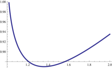
Figure 1: Plot of the effective potential $\Gamma[\bar{\rho}]$ illustrating an instability of the classical ground state at $\bar{\rho}=\bar{\rho}_{\rm cl}$. The minimum is reached at the mean-field ground state.

fig01

It is plotted in Fig. LABEL:fig01 versus $\bar{\rho}/\bar{\rho}_{\rm cl}$. The classical ground state $\bar{\rho}=\bar{\rho}_{\rm cl}$ (at the left end) is unstable and a stable minimum occurs at the mean-field value (the same as before) if $K_{0}>K_{*}$.

In the Lilliputian scaling regime $\Gamma[\bar{\rho}]$ is finite near the minimum and is given by a quadratic form which is positive defined, illustrating the global stability under fluctuations. The nonlinearity results in the string susceptibility $\gamma_{\rm str}=1/2$ for a cylinder and a torus as shown by Ambjørn, Y.M. (2017), (2021) which is quite different from $\gamma_{\rm str}=1$ of KPZ-DDK.

5 Fluctuations about the mean field

Expanding the effective action about the mean-field ground state, $\lambda^{ab}=\bar{\lambda}\delta^{ab}+\delta\lambda^{ab}(\omega)$ and $\rho=\bar{\rho}+\delta\rho(\omega)$, we observe the same stability of quadratic wavy fluctuations as about the classical ground state because of the background independence. We have a positive definite quadratic form for imaginary $\delta\lambda^{ab}$ and real $\delta\rho$. Again typical $\delta\lambda\sim 1/\Lambda$ so $\lambda^{ab}$ is localized. Thus only $\rho$ propagates to macroscopic distances and its smooth fluctuations are described by the usual Liouville action which is stable for $2<d<26$.

This is not however the whole story because of the private life of the fluctuating fields that occurs at the distances $\sim\Lambda^{-1}$ but is nevertheless observable as demonstrated by Y.M. (2021). I shall now describe this issue.

Let us set $\lambda^{z\bar{z}}=0$ and consider a simplified action ($\rho=\bar{\rho}{\,\rm e}^{\varphi}$)

$${\cal S}=\int\left[\frac{1}{4\pi b^{2}_{0}}\partial\varphi\bar{\partial}\varphi+\left(\lambda^{zz}\nabla\partial\varphi+\lambda^{\bar{z}\bar{z}}\bar{\nabla}\bar{\partial}\varphi\right)-d{\Lambda^{2}\bar{\rho}}{\,\rm e}^{\varphi}\lambda^{zz}\lambda^{\bar{z}\bar{z}}\right]\negthinspace,~{}~{}~{}b_{0}^{2}=\frac{6}{26-d}$$

where the last term with $\Lambda^{2}$ illustrates the statement of the previous paragraph about the localization. Integrating out $\lambda^{zz}$ and $\lambda^{\bar{z}\bar{z}}$ and integrating by parts, we find (only these two terms are independent)

$${\cal S}=\frac{1}{4\pi b_{0}^{2}}\int\left\{\partial\varphi\bar{\partial}\varphi+4\varepsilon{\,\rm e}^{-\varphi}\left[(\partial\bar{\partial}\varphi)^{2}+\partial\varphi\bar{\partial}\varphi\partial\bar{\partial}\varphi\right]\right\},\quad\varepsilon\propto\Lambda^{-2}$$

modulo boundary terms. The first additional term on the right-hand side appears already for Polyakov’s string from the Seeley expansion of the heat kernel but the second does not.

Thus, integrating over $X^{\mu}$, ghosts, Pauli-Villars’ regulators and $\lambda^{ab}$, we expect for the Nambu-Goto string the beyond Liouville action

$${\cal S}=\frac{1}{16\pi b_{0}^{2}}\int\sqrt{g}\left[g^{ab}\partial_{a}\varphi\partial_{b}\varphi+2m_{0}^{2}+\varepsilon R\left(R+Gg^{ab}\,\partial_{a}\varphi\partial_{b}\varphi\right)\right]$$

Here $\varphi=-\Delta^{-1}R$ becomes a local field in the conformal gauge. Once again, the $R^{2}$ appears already for the Polyakov string but the second (nonlocal) term with $G\neq 0$ is specific to the Nambu-Goto string.

Of course the higher-derivative terms are negligible classically for smooth metrics with $\varepsilon R\ll 1$, reproducing the Liouville action. However, the quartic derivative provides both a UV cutoff and also an interaction whose coupling constant is $\varepsilon$. We thus encounter uncertainties like $\varepsilon\times\varepsilon^{-1}$ so the higher-derivative terms revive quantumly. In other words the smallness of $\varepsilon$ is compensated by a change of the metric (the shift of $\varphi$) what is specific to the theory with diffeomorphism invariance.

The described procedure looks like an appearance of anomalies in quantum field theory. We may expect for this reason that possible yet higher-derivative terms will not change the results. An argument in favor of such a universality at $G=0$ was given by Y.M. (2021).

6 Comparison with KPZ-DDK

It is instructive to begin with the energy-momentum tensor of a scalar minimally coupled to gravity

$$-4b_{0}^{2}T_{ab}^{({\rm min})}=\partial_{a}\varphi\partial_{b}\varphi-\frac{1}{2}g_{ab}\partial^{c}\varphi\partial_{c}\varphi-\mu_{0}^{2}g_{ab}-\varepsilon\partial_{a}\varphi\partial_{b}\Delta\varphi-\varepsilon\partial_{a}\Delta\varphi\partial_{b}\varphi$$

$$\hskip 34.1433pt+\varepsilon g_{ab}\partial^{c}\varphi\partial_{c}\Delta\varphi+\frac{\varepsilon}{2}g_{ab}(\Delta\varphi)^{2}-G\varepsilon\partial_{a}\varphi\partial_{b}\varphi\Delta\varphi+G\frac{\varepsilon}{2}\partial_{a}\varphi\partial_{b}(\partial^{c}\varphi\partial_{c}\varphi)$$

$$\hskip 34.1433pt+G\frac{\varepsilon}{2}\partial_{a}(\partial^{c}\varphi\partial_{c}\varphi)\partial_{b}\varphi-G\frac{\varepsilon}{2}g_{ab}\partial^{c}\varphi\partial_{c}(\partial^{d}\varphi\partial_{d}\varphi)$$

The result by Gibbons, Pope, Solodukhin (2019) is reproduced at $G=0$.

Additional terms emerge for our diffeomorphism invariant action so the energy-momentum tensor as derived by Y.M. (2022) reads

$$-4b_{0}^{2}T_{ab} = -4b_{0}^{2}T_{ab}^{({\rm min})}-2(\partial_{a}\partial_{b}-g_{ab}\partial^{c}\partial_{c})(\varphi-\varepsilon\Delta\varphi+G\frac{\varepsilon}{2}g^{ab}\partial_{a}\varphi\partial_{b}\varphi)$$

$$+2G\varepsilon(\partial_{a}\partial_{b}-g_{ab}\partial^{c}\partial_{c})\frac{1}{\Delta}\partial^{d}(\partial_{d}\varphi\Delta\varphi)$$

It is conserved and traceless (!) thanks to diffeomorphism invariance in spite of $\varepsilon$ is dimensionful. Notice the nonlocality of the last term inherited from nonlocality of the covariant action.

The $T_{zz}$ component

$$-4b_{0}^{2}T_{zz}=(\partial\varphi)^{2}-2\varepsilon\partial\varphi\partial\Delta\varphi-2\partial^{2}(\varphi-\varepsilon\Delta\varphi)-G\varepsilon(\partial\varphi)^{2}\Delta\varphi$$

$$+G\varepsilon\Big{[}4\partial\varphi\partial({\,\rm e}^{-\varphi}\partial\varphi\bar{\partial}\varphi)-4\partial^{2}({\,\rm e}^{-\varphi}\partial\varphi\bar{\partial}\varphi)+\partial(\partial\varphi\Delta\varphi)+\frac{1}{\bar{\partial}}\partial^{2}(\bar{\partial}\varphi\Delta\varphi)\Big{]}$$

reproduces in two dimensions at $G=0$ the one by Kawai, Nakayama (1993).

Given $T_{zz}$ it is possible to perform á la DDK the computation of the conformal weight and the central charge at one loop about either the clasical of mean-field ground states. The results are the same because of the background independence. The operator products $T_{zz}(z){\,\rm e}^{\varphi(0)}$ and $T_{zz}(z)T_{zz}(0)$ are given at one loop by a bunch of diagrams most of which can be described by introducing

Figure 2: Diagrams for the operator products $T_{zz}(z){\,\rm e}^{\varphi(0)}$ or $T_{zz}(z)T_{zz}(0)$.

fi:2

an effective $T_{zz}$ for smooth fields similarly to DDK

$$-4b^{2}T_{zz}^{({\rm eff})}=(\partial\varphi)^{2}-2q\partial^{2}\varphi$$

For the conformal weight of ${\,\rm e}^{\varphi(0)}$, only this effective $T_{zz}$ contributes as $\varepsilon\to 0$ so we have $1=q-b^{2}$ as usual. For the central charge we have usual $6q^{2}/b^{2}+1$ from $T_{zz}^{({\rm eff})}$ but now the nonlocal term in $T_{zz}$ revives in the diagram k) and gives additionally $6G$. I shall momentarily return to this most interesting result. There is also a logarithmically divergent term whose appearance I link to the subtleties with conformal Ward identities for $G\neq 0$ because $T_{zz}$ is then not primary.

7 Algebraic check of DDK

To describe the one-loop renormalization in the standard way, we add Pauli-Villars’ regulators: Grassmann $Y$, $\bar{Y}$ (of mass squared $M^{2}$) and normal $Z$ (of mass squared $2M^{2}$) as proposed by Ambjørn, Y.M. (2017) at $\varepsilon=0$. This regularizes all involved divergences. To simplify formulas I keep below only $Y$ which is enough to compute finite parts. The regulator action reads

$${\cal S}_{\rm reg.}=\frac{1}{16\pi b_{0}^{2}}\int\sqrt{g}\left[g^{ab}\partial_{a}Y\partial_{b}Y+M^{2}Y^{2}+\varepsilon(\Delta Y)^{2}+G\varepsilon g^{ab}\partial_{a}Y\partial_{b}YR\right]$$

The regulators makes a contribution to the energy-momentum tensor which is quadratic in the regulator fields and local. The total energy-momentum tensor is conserved and traceless (!) in spite of the masses. We thus expect conformal invariance to be maintained quantumly what can be explicitly demonstrated by the one-loop and some two-loop calculations.

The renormalization of $b^{2}$ comes from the usual one-loop diagrams including tadpoles

$$\frac{1}{b^{2}}=\frac{1}{b_{0}^{2}}-\left(\frac{1}{6}-4+A+2G\int{\rm d}k^{2}\frac{\varepsilon}{(1+\varepsilon k^{2})}-\frac{1}{2}GA\right)+{\cal O}(b_{0}^{2})$$

Here $A(\varepsilon M^{2})\sim\sqrt{\varepsilon}M$ is the contribution of the tadpole.

The analogous one-loop renormalization of $q/b^{2}$ reads

$$\frac{q}{b^{2}}=\frac{1}{b_{0}^{2}}-\frac{1}{6}+2-\frac{1}{2}A-\frac{1}{2}G-G\int{\rm d}k^{2}\frac{\varepsilon}{(1+\varepsilon k^{2})}+\frac{1}{4}GA+{\cal O}(b_{0}^{2})$$

or, multiplying by $6b^{2}$,

$$\frac{6q^{2}}{b^{2}}=\left(\frac{q}{b^{2}}\right)^{2}\times 6b^{2}=\frac{6}{b_{0}^{2}}-1-6G+{\cal O}(b_{0}^{2})$$

This precisely confirms the above shift of the central charge by $6G$ obtained by the conformal field theory technique of DDK.

8 Conclusion

The classical (perturbative) ground state of the Nambu-Goto string is stable only for $d<2$. For $2<d<26$ the mean-field ground state is stable instead and we have the Lilliputian strings for $d>2$ versus Gulliver’s strings for $d\leq 2$. Higher-derivative terms in the beyond Liouville action for $\varphi$ revive, telling the Nambu-Goto and Polyakov strings apart. Two-dimensional conformal invariance is maintained by fluctuations in spite of dimensionful $\varepsilon$ but the central charge of $\varphi$ gets additional $6G$ at one loop.

All this is specific to the theory with diffeomorphism invariance. My final remark is about yet another diffeomorphism invariant theory – Gravity. The large-$d$ strings are described by bubble diagrams like the $O(N)$ sigma model but the large-$d$ gravity is described by planar diagrams like Yang-Mills as pointed out by Strominger (1981). This is the next level of complexity.

This work was supported by the Russian Science Foundation (Grant No.20-12-00195).

References

• [1] Ambjorn J., Makeenko Y. Scaling behavior of regularized bosonic strings, Phys. Rev. D 93 (2016) 066007 arXiv:1510.03390 [hep-th]; String theory as a Lilliputian world, Phys. Lett. B 756 (2016) 142 arXiv:1601.00540 [hep-th]; Stability of the nonperturbative bosonic string vacuum, Phys. Lett. B 770 (2017) 352 arXiv:1703.05382 [hep-th]; Scattering amplitudes of regularized bosonic strings, Phys. Rev. D 96 (2017) 086024 arXiv: 1704.03059 [hep-th]; The use of Pauli-Villars’ regularization in string theory, Int. J. Mod. Phys. A 32 (2017) 1750187 arXiv:1709.00995 [hep-th]; The susceptibility exponent of Nambu-Goto strings, Mod. Phys. Lett. A 36 (2021) 2150136 arXiv:2103.10259 [hep-th].
• [2] Makeenko Y. Mean field quantization of effective string, JHEP 1807 (2018) 104 arXiv:1802.07541 [hep-th]; Private life of the Liouville field that causes new anomalies in the Nambu-Goto string, Nucl. Phys. B 967 (2021) 115398 arXiv:2102.04753 [hep-th]; Opus on conformal symmetry of the Nambu-Goto versus Polyakov strings, arXiv:2204.10205 [hep-th].