Joint Privacy Enhancement and Quantization in Federated Learning

Abstract

fl is an emerging paradigm for training machine learning models using possibly private data available at edge devices. The distributed operation of FL gives rise to challenges that are not encountered in centralized machine learning, including the need to preserve the privacy of the local datasets, and the communication load due to the repeated exchange of updated models. These challenges are often tackled individually via techniques that induce some distortion on the updated models, e.g., local differential privacy (LDP) mechanisms and lossy compression. In this work we propose a method coined joint privacy enhancement and quantization (JoPEQ), which jointly implements lossy compression and privacy enhancement in federated learning (FL) settings. In particular, JoPEQ utilizes vector quantization based on random lattice, a universal compression technique whose byproduct distortion is statistically equivalent to additive noise. This distortion is leveraged to enhance privacy by augmenting the model updates with dedicated multivariate privacy preserving noise. We show that JoPEQ simultaneously quantizes data according to a required bit-rate while holding a desired privacy level, without notably affecting the utility of the learned model. This is shown via analytical LDP guarantees, distortion and convergence bounds derivation, and numerical studies. Finally, we empirically assert that JoPEQ demolishes common attacks known to exploit privacy leakage.

I Introduction

The unprecedented success of deep learning highly relies on the availability of data, often gathered by edge devices such as mobile phones, sensors, and vehicles. As such, data may be private, and there is a growing need to avoid leakage of private data while still being able to use it for training neural networks. fl [2, 3, 4, 5] is an emerging paradigm for training on edge devices, exploiting their computational capabilities [6]. FL avoids sharing the users’ data, as training is performed locally with periodic centralized aggregations of the models orchestrated by a server.

Learning in a federated manner is subject to several core challenges that are not encountered in traditional centralized machine learning [5, 4]. These include a repeated exchange of highly parameterized models between the server and the devices, possibly over rate-limited channels, notably loading the communication infrastructure and often resulting in considerable delays [7]. An additional challenge stems from the need to guarantee that the exchanged models preserve privacy with respect to the local datasets. It was recently shown that while learning on the edge does not involve data sharing, one can still extract private information, or even reconstruct the raw data, from the exchanged models updates, if these are not properly protected [8, 9, 10, 11].

Various methods have been proposed to tackle the above challenges: The communication overhead is often relaxed by reducing the volume of the model updates via lossy compression. This can be achieved by having each user transmit only part of its model updates by sparsifying or sub-sampling [12, 13, 14, 15, 16, 17]. An alternative approach discretizes the model updates via quantization, such that it is conveyed using a small number of bits [18, 19, 20, 21, 22, 23]. As for privacy preservation, the LDP framework is commonly adopted. LDP quantifies privacy leakage of a single data sample when some function of the local datasets, e.g., a trained model, is publicly available [24]. LDP can be boosted by corrupting the model updates with privacy preserving noise (PPN) [25], via splitting/shuffling [26] or dimension selection [27], and by exploiting the noise induced when communicating over a shared wireless channel [28, 29]. Prior works also studied the trade-offs between user privacy, utility, and transmission rate; providing utility [24] and convergence [30] bounds.

Several recent studies consider both challenges of compression and privacy in FL. The works [31, 32] quantize the local gradient with a differentially private 1-bit compressor. That is, the probability of each coordinate of the gradients to be encoded into one of two possible dictionary words is designed to satisfy the Gaussian mechanism; thus the communication burden is reduced while differential privacy (DP) is simultaneously guaranteed. However, these methods utilize fixed 1-bit quantizers, and cannot be configured into adaptable communication budget once available. In [33], the authors combine privacy and compression by converting the distortion induced by random lattice coding into a Gaussian noise which holds DP. To do so, they perturb the gradient by Gaussian noise prior to quantization, and the overall procedure then holds DP according to composition theorem of DP. The above works consider DP enhancements, providing users with privacy guarantees from untruthful adversaries, but fail to so for a potential untrusted FL third-party server; as can be guaranteed by LDP.

The recent work [34] proposed a compression method that holds LDP. This scheme, referred to in [34] as Minimum Variance Unbiased (MVU), utilizes dithered quantization to first transform the model updates into discrete-valued representations, that are subsequently perturbated to hold LDP. Yet, this scheme does not leverage the distortion already induced by quantization to enhance privacy via a joint design, but rather tackle each challenge separately in a cascaded fashion. Furthermore, the existing methods all individually perturb each sample of the model updates, thus not leveraging inter-sample correlations to enhance privacy. The fact that both compression and LDP enhancement typically involve the addition of some distortion to the model updates vector via, e.g., quantization or PPN, motivates the study of unified multivariate schemes for jointly boosting LDP and compression while maintaining the system utility in FL.

In this work we propose a dual-function mechanism for enhancing privacy while compressing the model updates in FL. Our proposed JoPEQ utilizes universal vector quantization techniques [35, 36], building upon their ability to transform the quantization distortion into an additive noise term with controllable variance regardless of the quantized data. We harness the resulting distortion as means to contribute to LDP enhancement, combining it with a dedicated additive PPN mechanism. For the latter, we specifically employ the highly useful yet less common approach of multivariate PPN [37], which can be naturally incorporated into established low-distortion vector quantization techniques. JoPEQ results in the local models recovered by the server simultaneously satisfying both desired LDP guarantees as well as bit-rate constraints, and does so without notably affecting the utility of the learned model. This is theoretically validated by both analytical LDP guarantees and convergence bound derivation. These findings are also consistently observed in our numerical study, which considers the federated training of different model architectures.

We design JoPEQ by extending the recently proposed FL quantization method of [21], which employs subtractive dithered quantization (SDQ) using randomized lattices for the local model weights. JoPEQ combines SDQ with a low-power PPN, carefully designed to yield an output that realizes an established LDP mechanism. We consider the multivariate multivariate $t$-distribution mechanism as well as the common scalar Laplace mechanism; both result in the local models being simultaneously quantized and private. We prove that the information recovered at the server side rigorously satisfies LDP guarantees, and characterize the regimes for which privacy can be achieved based solely on SDQ, i.e., while adding only a negligible level of artificial noise. Our numerical results demonstrate that JoPEQ achieves a lower level of overall distortion and yields more accurate models compared to using separate independent mechanisms for achieving compression and privacy, as well as to the scheme of [34]. Furthermore, we empirically demonstrate that JoPEQ is privacy preserving by demolishing the deep leakage from gradients (DLG) [8] and improved deep leakage from gradients (iDLG) [9] model inversion attacks, known to exploit privacy leakage and recover data samples from model updates.

The rest of this paper is organized as follows: Section II briefly reviews the FL system model and related preliminaries in quantization and privacy. Section III presents JoPEQ, theoretically analyzes its LDP guarantees and compression properties, deriving of distortion and convergence bounds. JoPEQ is numerically evaluated in Section IV, while Section V provides concluding remarks.

Throughout this paper, we use boldface lower-case letters for vectors, e.g., $\boldsymbol{x}$, boldface upper-case letters for matrices, e.g., $\boldsymbol{X}$, and calligraphic letters for sets, e.g., $\mathcal{X}$. The stochastic expectation, trace, variance, and $\ell_{1},\ell_{2}$ norms are denoted by $\mathds{E}\{\cdot\}$, $\operatorname{tr}(\cdot)$, $\operatorname*{\text{Var}}(\cdot)$ and ${\|\cdot\|}_{1},\|\cdot\|$, respectively, while $\mathbb{C}$ and $\mathbb{R}$ are the sets of complex and real numbers, respectively.

II System Model and Preliminaries

In this section we present the system model of FL with quantization and LDP constraints. We begin by recalling some relevant basics in FL and quantization in Subsections II-A-II-B respectively, after which we provide LDP preliminaries in Subsection II-C, and formulate our problem in Subsection II-D.

II-A Federated Learning

In FL, a server trains a model parameterized by $\boldsymbol{w}\in\mathbb{R}^{m}$ using data available at a group of $K$ users indexed by $1,\ldots,K$. These datasets, denoted $\mathcal{D}_{1},\dots,\mathcal{D}_{K}$, are assumed to be private. Thus, as opposed to conventional centralized learning where the server can use $\mathcal{D}=\bigcup_{k=1}^{K}\mathcal{D}_{k}$ to train $\boldsymbol{w}$, in FL the users cannot share their data with the server. Let $F_{k}(\boldsymbol{w})$ be the empirical risk of a model $\boldsymbol{w}$ evaluated over the dataset $\mathcal{D}_{k}$. The training goal is to recover the $m\times 1$ optimal weights vector $\boldsymbol{w}^{\rm opt}$ satisfying

$$\boldsymbol{w}^{\rm opt}=\operatorname*{arg\,min}_{\boldsymbol{w}}\left\{F(\boldsymbol{w})\triangleq\sum_{k=1}^{K}\alpha_{k}F_{k}\left(\boldsymbol{w}\right)\right\},$$ (1)

where the averaging coefficients are typically set to $\alpha_{k}=\frac{\lvert\mathcal{D}_{k}\rvert}{\lvert\mathcal{D}\rvert}$.

Generally speaking, FL involves the distribution of a global model to the users. Each user locally trains this global model using its own data, and sends back the model update [5]. The users thus do not directly expose their private data as training is performed locally. The server then aggregates the models into an updated global model and the procedure repeats iteratively.

Arguably the most common FL scheme is federated averaging (FedAvg) [2], where the server updates the global model by averaging the local models. Letting $\boldsymbol{w}_{t}$ denote the global parameters vector available at the server at time step $t$, the server shares $\boldsymbol{w}_{t}$ with the users, who each performs $\tau$ training iterations using its local $\mathcal{D}_{k}$ to update $\boldsymbol{w}_{t}$ into $\boldsymbol{w}^{k}_{t+\tau}$. The user then shares with the server the model update, i.e., $\boldsymbol{h}^{k}_{t+\tau}=\boldsymbol{w}^{k}_{t+\tau}-\boldsymbol{w}_{t}$. The server in turn sets the global model to be

$$\boldsymbol{w}_{t+\tau}\triangleq\boldsymbol{w}_{t}+\sum_{k=1}^{K}\alpha_{k}\boldsymbol{h}^{k}_{t+\tau}=\sum_{k=1}^{K}\alpha_{k}\boldsymbol{w}^{k}_{t+\tau},$$ (2)

where it is assumed for simplicity that all users participate in each FL round. The updated global model is again distributed to the users and the learning procedure continues.

When the local optimization at the users side is carried out using stochastic gradient descent (SGD), then FedAvg specializes the local SGD method [38]. In this case, each user of index $k$ sets $\boldsymbol{w}_{t}^{k}=\boldsymbol{w}_{t}$, and updates its local model via

$$\boldsymbol{w}^{k}_{t+1}\xleftarrow{}\boldsymbol{w}^{k}_{t}-\eta_{t}\nabla F^{i^{k}_{t}}_{k}\left(\boldsymbol{w}^{k}_{t}\right),$$ (3)

where $i^{k}_{t}$ is the sample index chosen uniformly from $\mathcal{D}_{k}$, and $\eta_{t}$ is the step-size. The fact that FL involves the users sharing their updated local models $\boldsymbol{w}^{k}_{t+\tau}$ with the server gives rise to the core challenges in terms of communication overload and privacy considerations. This motivates the incorporation of quantization and privacy enhancement techniques, discussed in the following subsections.

II-B Quantization Preliminaries

Vector quantization is the encoding of a set of continuous-amplitude quantities into a finite-bit representation [39]. The design of vector quantizers often relies on statistical modelling of the vector to be quantized [40, Ch. 23], which is likely to be unavailable in FL [21]. Vector quantizers which are invariant of the underlying distribution are referred to as universal vector quantizers; a leading approach to implement such quantizers is based on lattice quantization [35]:

Definition II.1 (Lattice Quantizer).

A lattice quantizer of dimension $L\in\mathbb{Z}^{+}$ and generator matrix $\boldsymbol{G}\ \in\mathbb{R}^{L\times L}$ maps $\boldsymbol{x}\in\mathbb{R}^{L}$ into a discrete representation $Q_{\mathcal{L}}(\boldsymbol{x})$ by selecting the nearest point in the lattice $\mathcal{L}\triangleq\{\boldsymbol{G}\boldsymbol{l}:\boldsymbol{l}\in\mathbb{Z}^{L}\}$, i.e.,

$$Q_{\mathcal{L}}(\boldsymbol{x})=\mathop{\arg\min}_{\boldsymbol{z}\in\mathcal{L}}\|\boldsymbol{x}-\boldsymbol{z}\|.$$ (4)

To apply $Q_{\mathcal{L}}$ to a vector $\boldsymbol{x}\in\mathbb{R}^{ML}$, it is divided into $[\boldsymbol{x}_{1},\ldots,\boldsymbol{x}_{M}]^{T}$, and each sub-vector is quantized separately. A lattice $\mathcal{L}$ partitions $\mathbb{R}^{L}$ into cells centered around the lattice points, where the basic cell is $\mathcal{P}_{0}=\{\boldsymbol{x}:Q_{\mathcal{L}}(\boldsymbol{x})=\mathbf{0}\}$. The number of lattice points in $\mathcal{L}$ is countable but infinite. Thus, to obtain a finite-bit representation, it is common to restrict $\mathcal{L}$ to include only points in a given sphere of radius $\gamma$, and the number of lattice points dictates the number of bits per sample $R$. An event in which the input does not reside in this sphere is referred to as overloading, and quantizers are typically designed to avoid this [39]. In the special case of $L=1$ with $\boldsymbol{G}=\Delta_{\rm Q}>0$, $Q_{\mathcal{L}}(\cdot)$ specializes conventional scalar uniform quantization $Q(\cdot)$:

Definition II.2 (Uniform Quantizer).

A mid-tread scalar uniform quantizer with support $\gamma$ and spacing $\Delta_{\rm Q}$ is defined as

$$Q(x)=\begin{cases}\Delta_{\rm Q}\left\lfloor\frac{x}{\Delta_{\rm Q}}+\frac{1}{2}\right\rfloor&\text{if }x<\lvert\gamma\rvert\\ \operatorname*{\text{sign}}(x)\cdot\gamma&\text{else},\end{cases}$$ (5)

where $R~{}=~{}\log_{2}\big{(}2\gamma/\Delta_{\rm Q}\big{)}$ bits are used to represent $x$.

The straightforward application of lattice quantization yields a distortion term $\boldsymbol{e}\triangleq Q_{\mathcal{L}}(\boldsymbol{x})-\boldsymbol{x}$ that is deterministically determined by $\boldsymbol{x}$. It is thus often combined with probabilistic quantization techniques, and particularly with dithered quantization (DQ) and SDQ [41, 42], defined below:

Definition II.3 (DQ).

The dithered lattice quantization of $\boldsymbol{x}\in\mathbb{R}^{L}$ is given by

$$Q^{\rm DQ}_{\mathcal{L}}(\boldsymbol{x})=Q_{\mathcal{L}}(\boldsymbol{x}+\boldsymbol{d}),$$ (6)

where $\boldsymbol{d}$ denotes the dither signal, which is independent of $\boldsymbol{x}$ and is uniformly distributed over the basic lattice cell $\mathcal{P}_{0}$.

Definition II.4 (SDQ).

The subtractive dithered lattice quantization of $\boldsymbol{x}\in\mathbb{R}^{L}$ is given by

$$Q^{\rm SDQ}_{\mathcal{L}}(\boldsymbol{x})=Q^{\rm DQ}_{\mathcal{L}}(\boldsymbol{x})-\boldsymbol{d}=Q_{\mathcal{L}}(\boldsymbol{x}+\boldsymbol{d})-\boldsymbol{d}.$$ (7)

A key property of SDQ stems from the fact that its resulting distortion can be made independent of the quantized value. This arises from the following theorem, stated in [42, 36]:

Theorem II.5.

For a set of $L\times 1$ vectors $\{\boldsymbol{x}_{i}\}_{i=1}^{M}$ within the lattice support, i.e., $\Pr(\|\boldsymbol{x}_{i}\|\leq\gamma)=1$, the distortion vectors $\boldsymbol{e}_{i}\triangleq Q^{\rm SDQ}_{\mathcal{L}}(\boldsymbol{x}_{i})-\boldsymbol{x}_{i}$ are i.i.d., uniformly distributed over $\mathcal{P}_{0}$ and mutually independent of $\{\boldsymbol{x}_{i}\}_{i=1}^{M}$.

Theorem II.5 implies that when the quantizer is not overloaded, the distortion induced by SDQ can be effectively modeled as white noise uniformly distributed over $\mathcal{P}_{0}$.

II-C Local Differential Privacy Preliminaries

One of the main motivations for FL is the need to preserve the privacy of the users’ data. Nonetheless, the concealment of the dataset of the $k$th user, $\mathcal{D}_{k}$, in favor of sharing the weights trained using this data $\boldsymbol{w}_{t}^{k}$ was shown to be potentially leaky [8, 9, 10, 11]. Therefore, to satisfy the privacy requirements of FL, initiated privacy mechanisms are necessary [31].

Considering a users-server setting, privacy is commonly quantified in terms of DP [43, 44] and LDP [45, 46]. While both provide users with privacy guarantees from untruthful adversaries, the former further assumes a trusted third-party server. As this assumption does not necessarily hold for FL, to alleviate the privacy concerns of each user the commonly adopted framework is that of LDP, defined as follows:

Definition II.6 ($\epsilon$-LDP [47]).

A randomized mechanism $\mathcal{M}$ satisfies $\epsilon$-LDP if for any pairs of input values $v,v^{\prime}$ in the domain of $\mathcal{M}$ and for any possible output $y$ in it, it holds that

$$\Pr[\mathcal{M}(v)=y]\leq e^{\epsilon}\Pr[\mathcal{M}(v^{\prime})=y].$$ (8)

Definition II.6 can be interpreted as a bundle between stochasticity and privacy: if two different inputs are probable (up to some margin or privacy budget) to be associated with the same algorithm output, then privacy is preserved as each data sample is not uniquely distinguishable. A smaller $\epsilon$ means stronger privacy protection, and vice versa. A common mechanism to achieve $\epsilon$-LDP is based on Laplacian PPN. By letting $\operatorname*{\text{Laplace}}\left(\mu,b\right)$ be the Laplace distribution with location $\mu$ and scale $b$, the Laplace mechanism is defined as follows:

Theorem II.7 ([48]).

Given any function $f:\mathds{D}\to\mathbb{R}^{d}$ where $\mathds{D}$ is a domain of datasets, the Laplace mechanism defined as

$$\mathcal{M}^{\rm Laplace}\left(f(x),\epsilon\right)=f(x)+{\left[z_{1},\dots,z_{d}\right]}^{T},$$ (9)

is $\epsilon$-LDP. In (9), $z_{i}\overset{\acs{iid}}{\sim}\operatorname*{\text{Laplace}}\left(0,\Delta f/\epsilon\right)$, with

$$\Delta f\triangleq\max_{x,y\in\mathds{D}}\left\|f(x)-f(y)\right\|.$$

Theorem II.7 concerns multivariate data, yet uses i.i.d. univariate Laplace random perturbations, and thus fails to exploit spatial correlations in the data for privacy. In particular, the statistical dependence between different variables in each data sample can be exploited for lowering the overall added distortion while keeping the privacy budget unchanged [37, 49, 50, 51]. This is achieved using high-dimensional privacy preserving mechanisms, which engage multivariate PPNs. While the straightforward multivariate Laplacian PPN fails to satisfy $\epsilon$-LDP when $d>1$ [37], one can guarantee privacy by introducing multivariate perturbations obeying the $t$-distribution. In particular, letting $\mathbf{t}^{d}_{\nu}(\boldsymbol{\mu},\mathbf{\Sigma})$ denote the $d$-dimensional $t$-distribution with location, scale matrix, and degrees-of-freedom $\boldsymbol{\mu}$, $\mathbf{\Sigma}$, and $\nu$ respectively, such a PPN satisfies LDP guarantees as stated in the following theorem:

Theorem II.8 ([37]).

Given any function $f:\mathds{D}\to\mathbb{R}^{d}$, define

$$\mathcal{M}^{\rm t\text{-}dist}\left(f(x),\epsilon\right)=f(x)+\mathbf{t};\quad\mathbf{t}{\sim}\mathbf{t}^{d}_{\nu}(\boldsymbol{\mu},\mathbf{\Sigma}).$$ (10)

Then, $\mathcal{M}^{\rm t\text{-}dist}$ satisfies $\epsilon$-LDP, for

$$\exp(\epsilon)={\left[\frac{1+c^{2}/\nu}{1+(c-\Delta)^{2}/\nu}\right]}^{(\nu+d)^{2}},$$ (11)

where here $c\triangleq\frac{1}{2}\left(\Delta+\sqrt{\Delta^{2}+4\nu}\right)$ and

$$\Delta\triangleq\max_{x,y\in\mathds{D}}\|\mathbf{\Sigma}^{-1/2}\left(f(x)-f(y)\right)\|.$$

The mapping (10) is referred to as multivariate $t$-distribution mechanism. Both Laplace and multivariate $t$-distribution mechanisms use PPN to guarantee privacy. While the former is more commonly used in FL, e.g., [52], the latter further leverages spatial correlation in multivariate data to enable privacy enhancement with lower power perturbations [37].

II-D Problem Formulation

Our goal is to design a mechanism which jointly meets both quantization and privacy constraints in FL. Since users are unlikely to have prior knowledge of the model parameters distribution, we are interested in methods which are universal. Such schemes can be formulated as mappings of the local updates $\boldsymbol{h}_{t}^{k}\in\mathbb{R}^{d}$ at the $k$th user into $\tilde{\boldsymbol{h}}_{t}^{k}\in\mathbb{R}^{d}$ available at the server, while meeting the following requirements:

1. Privacy: the mapping of $\boldsymbol{h}_{t}^{k}$ into $\tilde{\boldsymbol{h}}_{t}^{k}$ must be $\epsilon$-LDP with respect to $\mathcal{D}_{k}$ for a given privacy budget $\epsilon$.

2. Compression: the conveying of $\tilde{\boldsymbol{h}}_{t}^{k}$ from the user to the server should involve at most $R$ bits per sample.

3. Universality: the scheme must be invariant to the distribution of $\boldsymbol{h}_{t}^{k}$.

Notice that by R1 we are focusing on achieving LDP in each time instance, i.e., for each $t$. This is known to enable privacy enhancement in multi-round FL training procedures [26].

Evidently, requirements R1-R3 can be satisfied by first adding PPN to meet R1, followed by universal quantization to satisfy R2-R3, as both techniques are invariant to the distribution of $\boldsymbol{h}_{t}^{k}$. However, these FL quantization and privacy boosting schemes can be modelled as corrupting the weights with some random noise (e.g., Thm. II.5 for SDQ, Thm. II.7 for Laplace mechanism, and Thm. II.8 for multivariate $t$-distribution mechanism). Thus, using separate mechanisms may result in an overall noise which degrades the accuracy of the trained model beyond that needed to meet R1-R3. Based on these observations, in the sequel we study a joint design.

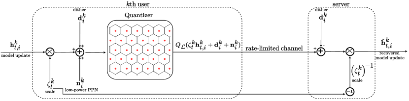
Figure 1: Overview of JoPEQ, where the left dashed box represents the encoding by the $k$th user, while the right dashed box describes the server decoding.

III Joint Privacy Enhancement and Quantization

In this section we introduce JoPEQ, deriving its steps in Subsection III-A, after which we provide an analysis and discuss its properties in Subsections III-B-III-C, respectively.

III-A JoPEQ

We design JoPEQ to exploit the inherent stochasticity of probabilistic quantized FL to enhance privacy, relaxing the need to manually introduce possibly dominant PPN separately. We tackle both FL challenges of communication overload and privacy consideration simultaneously by employing the unique distortion properties of SDQ for implementing established privacy enhancing mechanisms. This is achieved by first corrupting the model updates $\boldsymbol{h}_{t}^{k}$ with a low-power PPN followed by compressing via SDQ. The PPN is carefully designed such that the local model available at the server holds a desirable LDP preserving mechanism, e.g., multivariate $t$-distribution mechanism or Laplace mechanism, yielding an output that is both quantized and privacy preserving.

JoPEQ is divided into two main stages of encoding and decoding, carried out by the user and the server, respectively, with a preliminary initialization stage conducted when the FL procedure commences. These steps are detailed below and illustrated in Fig. 1. As the mechanism description is identical for each of the local users participating in the FL process, we henceforth focus only on the $k$th user.

III-A1 Initialization

The first step sets of the privacy budget $\epsilon$, dictated by the application requirements, and the compression scheme parameters, that are based on [21]. The latter includes sharing a common seed $s_{k}$ between each user and the server, that serves as a source of common randomness; fixing the lattice dimension $L$ and its radius $\gamma$; and forming the generator matrix $\mathbf{G}$ (that dictates the lattice $\mathcal{L}$ and its basic cell $\mathcal{P}_{0}$), which is determined by the bit-rate $R$ [53, Ch. 2].

III-A2 Encoding

The encoding stage takes place at the user sides when the round of local training is finished and the model updates $\boldsymbol{h}_{t}^{k}$ are ready to be transmitted. The updates are encoded into finite bit representations using a combination of SDQ and the addition of a carefully designed PPN to result with an $\epsilon$-LDP mechanism.

Quantization: JoPEQ builds upon the compression scheme of [21], which is implemented via scaling followed by SDQ (Def. II.4) with lattice quantization (Def. II.1). In particular, this operation involves the scaling of $\boldsymbol{h}^{k}_{t}$ by a coefficient $\zeta_{t}^{k}$ and its division into $M\triangleq\left\lceil\frac{d}{L}\right\rceil$ distinct $L\times 1$ sub-vectors, applying the $L$-dimensional lattice quantizer on each $\{\zeta_{t}^{k}\boldsymbol{h}_{t,i}^{k}\}_{i=1}^{M}$. The scaling coefficient $\zeta_{t}^{k}$ guarantees that the quantizer is unlikely to be overloaded, i.e., that the sub-vectors lie inside the unit $L$-ball with high probability. A candidate setting is thus $\zeta_{t}^{k}=\left(\frac{3}{\sqrt{M}}\|\boldsymbol{h}^{k}_{t}\|\right)^{-1}$, approaching three times the standard deviation of the sub-vectors when they are zero-mean and i.i.d., thus assuring no overloading with probability of over $88\%$ by Chebyshev’s inequality [54].

To implement SDQ, the user randomizes the dither signals $\boldsymbol{d}_{i}^{k}\in\mathbb{R}^{L}$ independently of $\boldsymbol{h}^{k}_{t,i}$ for each $i\in\{1,\ldots,M\}$, where $\boldsymbol{d}_{i}^{k}$ is uniformly distributed over $\mathcal{P}_{0}$. Unlike [21], which considers solely compression, JoPEQ does not directly quantize $\boldsymbol{h}^{k}_{t,i}$, but rather first distorts it with PPN $\boldsymbol{n}^{k}_{i}$ for enhancing privacy. The vectors which are conveyed from the $k$th user to the server are thus $\{Q_{\mathcal{L}}(\zeta_{t}^{k}\boldsymbol{h}^{k}_{t,i}+\boldsymbol{d}^{k}_{i}+\boldsymbol{n}^{k}_{i})\}_{i=1}^{M}$ at a bit-rate of at most $R$ bits per sample due the lattice quantizer $Q_{\mathcal{L}}(\cdot)$; the associated overhead in conveying the scalar $\zeta_{t}^{k}$ is assumed to be negligible compared to conveying $\boldsymbol{h}_{t}^{k}$.

Privacy enhancement: The PPN signals $\{\boldsymbol{n}^{k}_{i}\}^{M}_{i=1}$ are randomized by the $k$th user. Unlike the dither, which the server can also generate with the shared seed, the PPN uses a local seed and thus cannot be recreated by the server. The PPN $\boldsymbol{n}^{k}_{i}$ is generated for each $i\in\{1,\dots,M\}$ in an i.i.d. fashion from a multivariate distribution with the characteristic function $\Phi_{\boldsymbol{n}}:\mathbb{R}^{L}\mapsto\mathbb{C}$. We propose two settings for $\Phi_{\boldsymbol{n}}$ in Theorems III.1-III.2, for which JoPEQ realizes a multivariate $t$-distribution mechanism and a Laplace mechanism, respectively.

III-A3 Decoding

The server receives the DQ of $\{\zeta_{t}^{k}\boldsymbol{h}^{k}_{t,i}+\boldsymbol{n}^{k}_{i}\}_{i=1}^{M}$, which can be modeled as a distorted scaled version of $\{\boldsymbol{h}^{k}_{t,i}\}_{i=1}^{M}$. Since the server has access to the shared seed $s_{k}$ used to generate the dither and also to the scaling coefficient $\zeta_{t}^{k}$, this distortion can reduced by implementing SDQ [42] and re-scaling. This results in the server obtaining $\tilde{\boldsymbol{h}}^{k}_{t}$ as the stacking of $\{\tilde{\boldsymbol{h}}^{k}_{t,i}\}_{i=1}^{M}$ given by

$$\tilde{\boldsymbol{h}}^{k}_{t,i} =(\zeta_{t}^{k})^{-1}\cdot\left(Q_{\mathcal{L}}(\zeta_{t}^{k}\boldsymbol{h}^{k}_{t,i}+\boldsymbol{n}^{k}_{i}+\boldsymbol{d}^{k}_{i})-\boldsymbol{d}^{k}_{i}\right)$$ (12)

$$=(\zeta_{t}^{k})^{-1}\cdot Q_{\mathcal{L}}^{\rm SDQ}(\zeta_{t}^{k}\boldsymbol{h}^{k}_{t,i}+\boldsymbol{n}^{k}_{i}).$$ (13)

The decoding procedure of JoPEQ is carried out at the server side, from whom privacy should be preserved. Decoding involves dither subtraction and inverse scaling. Dither subtraction is known to reduce the variance of the overall distortion [42], and is thus beneficial in terms of improving the accuracy of the global model aggregated via FedAvg [21]. Yet, since (12) is less distorted, and thus potentially more leaky, than $\{(\zeta_{t}^{k})^{-1}\cdot Q_{\mathcal{L}}(\zeta_{t}^{k}\boldsymbol{h}^{k}_{t,i}+\boldsymbol{n}^{k}_{i}+\boldsymbol{d}^{k}_{i})\}_{i=1}^{M}$ due to dither subtraction, we focus our privacy enhancement and analysis on $\tilde{\boldsymbol{h}}^{k}_{t}$. The overall algorithm is summarized below as Algorithm 1.

Data: Local model updates at the $k$th user at time step $t$, $\boldsymbol{h}^{k}_{t}$, decomposed into $\{\boldsymbol{h}^{k}_{t,i}\}_{i=1}^{M}$;

Result: Representation of local model updates $\tilde{\boldsymbol{h}}_{t}^{k}$ to be aggregated using FedAvg;

Initialization:

1      Shared seed $s_{k}$, lattice $\mathcal{L}$, and privacy budget $\epsilon$;

2

Encode (at the $k$th user side, for each $i$):

3      Randomize the dither signal $\boldsymbol{d}^{k}_{i}$, uniformly distributed over $\mathcal{P}_{0}$, using seed $s_{k}$;

4       Randomize the PPN signal $\boldsymbol{n}^{k}_{i}$, obeying the characteristic function $\Phi_{\boldsymbol{n}}$;

5       Convey $Q_{\mathcal{L}}(\zeta_{t}^{k}\boldsymbol{h}^{k}_{t,i}+\boldsymbol{d}^{k}_{i}+\boldsymbol{n}^{k}_{i})$ and $\zeta_{t}^{k}$ to server;

6

Decode (at the server side, for each $i$):

7      Recreate the dither signal $\boldsymbol{d}^{k}_{i}$ using seed $s_{k}$;

8       Compute $\tilde{\boldsymbol{h}}^{k}_{t,i}$ using (13);

9

Algorithm 1 JoPEQ

III-B Analysis

Next, we analyze the performance of JoPEQ, characterizing its privacy and compression guarantees, after which we study its associated distortion and convergence properties.

III-B1 Privacy

The encoding procedure of JoPEQ is designed to jointly support privacy by adding PPN and compression via lattice quantization. When scaling by $\zeta_{t}^{k}$ yields vanishing overloading probability, the setting of the PPN characteristic function can guarantee that $\tilde{\boldsymbol{h}}^{k}_{t,i}$ is equivalent to the model updates $\boldsymbol{h}^{k}_{t,i}$ corrupted by a desired distortion profile. This is stated in the following theorem:

Theorem III.1.

Given a fixed $\zeta_{t}^{k}$ that yields vanishing overloading probability, let the PPN be generated with the characteristic function $\Phi_{\boldsymbol{n}}(\boldsymbol{t})$, which for all $\boldsymbol{t}\in\mathbb{R}^{L}$ is defined as:

$$\Phi_{\boldsymbol{n}}(\boldsymbol{t})={\left(\int_{\mathcal{P}_{0}}\frac{\cos\left({\boldsymbol{t}}^{T}\boldsymbol{e}\right)}{\lvert\mathcal{P}_{0}\rvert}d\boldsymbol{e}\right)}^{-1}\times\\ \exp(i\boldsymbol{t}^{T}\boldsymbol{\mu})\frac{\|\sqrt{\nu}\boldsymbol{\Sigma}^{1/2}\boldsymbol{t}\|^{\nu/2}}{2^{\nu/2-1}\Gamma(\nu/2)}K_{\nu/2}\left(\|\sqrt{\nu}\boldsymbol{\Sigma}^{1/2}\boldsymbol{t}\|\right),$$ (14)

where $\Gamma(\cdot),K(\cdot)$ are the gamma and the third kind modified Bessel functions respectively. Then, the distortion at the output of JoPEQ, $\tilde{\boldsymbol{h}}^{k}_{t,i}-\boldsymbol{h}^{k}_{t,i}$, is mutually independent of $\boldsymbol{h}^{k}_{t,i}$ and obeys an i.i.d. $\mathbf{t}^{d}_{\nu}(\boldsymbol{\mu},\mathbf{\Sigma})$ distribution, which satisfies (11).

Proof:

The proof is given in Appendix -A. ∎

JoPEQ can also hold other privacy mechanisms, such as the Laplace mechanism. The latter is commonly used when working with scalar quantities, instead of the multivariate $t$-distribution mechanism which is more complex yet is capable of achieving lower distortion for the same privacy budget [37]. The necessary adaptation for its implementing Laplace mechanism by JoPEQ is formulated in the following theorem.

Theorem III.2.

Given a fixed $\zeta_{t}^{k}$ that yields vanishing overloading probability, let the PPN be generated with the characteristic function $\Phi_{\boldsymbol{n}}(\boldsymbol{t})$, $\boldsymbol{t}=\left[t_{1}\dots,t_{L}\right]^{T}\in\mathbb{R}^{L}$, given by:

$$\Phi_{\boldsymbol{n}}(\boldsymbol{t})={\left(\int_{\mathcal{P}_{0}}\frac{\cos\left({\boldsymbol{t}}^{T}\boldsymbol{e}\right)}{\lvert\mathcal{P}_{0}\rvert}d\boldsymbol{e}\right)}^{-1}\prod_{l=1}^{L}\frac{1}{{1+{\left(2t_{l}/\epsilon\right)}^{2}}}.$$ (15)

Then, the distortion at the output of JoPEQ, $\tilde{\boldsymbol{h}}^{k}_{t,i}-\boldsymbol{h}^{k}_{t,i}$, is mutually independent of $\boldsymbol{h}^{k}_{t,i}$ and its entries obey an i.i.d. $\operatorname*{\text{Laplace}}\left(0,{2}/{\epsilon}\right)$ distribution.

Proof:

The proof is given in Appendix -B. ∎

As shown in Appendices -A and -B, the characteristic functions in (14) and (15) are respectively obtained by exploiting the mutual independence of the SDQ error and the quantized value. Hence, our ability to rigorously support privacy is a direct consequence of using universal dithered quantization.

Theorems III.1-III.2 imply that the unified effect of the PPN and SDQ in JoPEQ can implement established LDP mechanisms. This is achieved in addition to compressing $\boldsymbol{h}^{k}_{t}$. Thus, combining Theorems III.1-III.2 with Theorems II.7-II.8 guarantees privacy as stated in the following corollary:

Corollary 1.

JoPEQ with multivariate PPN randomized via either (14) or (15) is $\epsilon$-LDP with respect to $\mathcal{D}_{k}$.

III-B2 Compression

While Corollary 1 focuses on the privacy guarantees of JoPEQ, Algorithm 1 also implements compression. In particular, JoPEQ is designed to exploit the distortion induced by quantization, which is dictated by the bit-rate $R$, for privacy enhancement, such that PPN is only added to complement the remaining level of perturbation needed for a desired privacy budget $\epsilon$ to be obtained. In fact, in some settings one can meet the privacy guarantees based almost solely on the distortion induced by SDQ, while using PPN with infinitesimally small variance, as stated below:

Theorem III.3.

When the lattice generator matrix $\boldsymbol{G}$ equals the $L\times L$ identity matrix (up to some scalar factor), then JoPEQ with bit-rate $R$ and with PPN of an infinitesimally small variance randomized from (15) is $\epsilon$-LDP when

$$5\approx\sqrt{24}\leq \gamma\epsilon/2^{R}.$$ (16)

Proof:

The proof is given in Appendix -C. ∎

The setting for which Theorem III.3 is formulated, i.e., that $\boldsymbol{G}$ is the scaled identity matrix, implies that it uses uniform scalar quantizers, as in, e.g., [18, 19]. While Theorem III.3 rigorously holds for a specific family of quantizers, it reveals how JoPEQ jointly balances its privacy and compression requirements R1-R2: the stronger the privacy requirement is (smaller $\epsilon$), the more coarse the quantization (smaller $R$) that can support it without effectively injecting PPN.

III-B3 Weights Distortion

In the end of its pipeline, JoPEQ results with an $\epsilon$-LDP mechanism applied to the model updates. Consequently, it inherently induces some distortion, being introduced in the FL training process, namely, the model update $\boldsymbol{h}^{k}_{t}$ is transformed into the distorted version $\tilde{\boldsymbol{h}}^{k}_{t}$. Accordingly, the global model of (2), $\boldsymbol{w}_{t+\tau}$, which is the desired outcome of FedAvg, is changed into

$$\tilde{\boldsymbol{w}}_{t+\tau}\triangleq\boldsymbol{w}_{t}+\sum_{k=1}^{K}\alpha_{k}\tilde{\boldsymbol{h}}^{k}_{t+\tau}.$$ (17)

We next show that, under common assumptions used in FL analysis, the effect of the distortion in Theorems III.1-III.2 can be mitigated while recovering the desired $\boldsymbol{w}_{t+\tau}$ as $\tilde{\boldsymbol{w}}_{t+\tau}$. Thus, the accuracy of the global learned model can be maintained, despite the excessive distortion induced by JoPEQ.

To begin, set the scaling factor to $\zeta_{t}^{k}=\left(\frac{3}{\sqrt{M}}\|\boldsymbol{h}^{k}_{t}\|\right)^{-1}$ and define $\sigma^{2}$ as the variance of the LDP mechanism, e.g., $\sigma^{2}=\nu\frac{\operatorname{tr}\left(\mathbf{\Sigma}\right)}{\nu-2}$ for the multivariate $t$-distribution mechanism. Next, we adopt the following assumptions on the local datasets and on the stochastic gradient vector $\nabla F_{k}^{i}\left(\boldsymbol{w}\right)$:

1. Each dataset $\mathcal{D}_{k}$ is comprised i.i.d. samples. However, different datasets can be statistically heterogeneous, i.e., arise from different distributions.

2. The expected squared $\ell_{2}$-norm of the vector $\nabla F_{k}^{i}\left(\boldsymbol{w}\right)$ in (3) is bounded by some $\xi^{2}_{k}>0$ for all $\boldsymbol{w}\in\mathbb{R}^{m}$.

The statistical heterogeneity in Assumption AS1 is a common characteristic of FL [3, 4, 55]. It is consistent with Requirement R3, which does not impose any specific distribution structure on the underlying statistics of the training data. Such heterogeneity implies that the loss surfaces can differ between users, hence the dependence on $k$ in Assumption AS2, often employed in distributed learning studies [21, 56, 38, 57].

We can now bound the distance between the recovered model $\tilde{\boldsymbol{w}}_{t+\tau}$ of (17) and the desired one $\boldsymbol{w}_{t+\tau}$, as stated next:

Theorem III.4.

When AS2 holds, the mean-squared distance between $\tilde{\boldsymbol{w}}_{t+\tau}$ and $\boldsymbol{w}_{t+\tau}$ satisfies

$$\mathds{E}\left\{\|\tilde{\boldsymbol{w}}_{t+\tau}-\boldsymbol{w}_{t+\tau}\|^{2}\right\}\leq 9\tau\sigma^{2}\left(\sum_{t^{\prime}=t}^{t+\tau-1}\eta_{t^{\prime}}^{2}\right)\sum_{k=1}^{K}\alpha_{k}^{2}\xi^{2}_{k},$$ (18)

Proof:

The proof is given in Appendix -D. ∎

Theorem III.4 implicitly suggests that when the aggregation is fairly balanced, the recovered model can be made arbitrarily close to the desired one by increasing the number of edge users participating in the FL training procedure. Taking conventional averaging as an example, where each $\alpha_{k}=1/K$, we get that (18) decreases as $1/K$. Furthermore, if $\max\alpha_{k}\propto 1/{K^{c}}$ for some $c>1/2$ , which essentially means that the updated model is dominated by a small part of the participating users, then the distortion vanishes in the aggregation process as $K$ grows. Besides, when the step-size $\eta_{t}$ gradually decreases, which is known to contribute to the convergence of FL [38, 56], it follows from Theorem III.4 that the distortion decreases accordingly, further revealing its effect as the FL iterations progress, discussed next.

III-B4 Federated Learning Convergence

To study the convergence of FedAvg with JoPEQ, we further introduce the following assumptions, inspired by FL convergence studies in, e.g., [21, 56, 38]:

1. The local objective functions $\{F_{k}(\cdot)\}^{K}_{k=1}$ are all $\rho_{s}$-smooth, i.e., for all $\boldsymbol{w}_{1},\boldsymbol{w}_{2}\in\mathbb{R}^{m}$ it holds that

   $$F_{k}(\boldsymbol{w}_{1})-F_{k}(\boldsymbol{w}_{2})\leq(\boldsymbol{w}_{1}-\boldsymbol{w}_{2})^{T}\nabla F_{k}(\boldsymbol{w}_{2})\\ +\frac{1}{2}\rho_{s}{\|\boldsymbol{w}_{1}-\boldsymbol{w}_{2}\|}^{2}.$$

2. The local objective functions $\{F_{k}(\cdot)\}^{K}_{k=1}$ are all $\rho_{c}$-strongly convex, i.e., for all $\boldsymbol{w}_{1},\boldsymbol{w}_{2}\in\mathbb{R}^{m}$ it holds that

   $$F_{k}(\boldsymbol{w}_{1})-F_{k}(\boldsymbol{w}_{2})\geq(\boldsymbol{w}_{1}-\boldsymbol{w}_{2})^{T}\nabla F_{k}(\boldsymbol{w}_{2})\\ +\frac{1}{2}\rho_{c}{\|\boldsymbol{w}_{1}-\boldsymbol{w}_{2}\|}^{2}.$$

Assumptions 3-4 hold for a range of objective functions used in FL, including $\ell_{2}$-norm regularized linear regression and logistic regression [21]. To proceed, following AS1 and as in [56, 21], we define the heterogeneity gap,

$$\psi\triangleq F(\boldsymbol{w}^{\rm opt})-\sum_{k=1}^{K}\alpha_{k}\min_{\boldsymbol{w}}F_{k}(\boldsymbol{w}),$$ (19)

where $\boldsymbol{w}^{\rm opt}$ is defined in (1). Notice that (19) quantifies the degree of heterogeneity: if the training data originates from the same distribution, $\psi$ tends to zero as the training size grows, and is positive otherwise.

The following theorem characterizes JoPEQ convergence in conventional FL with local SGD training:

Theorem III.5.

Set $\varphi\triangleq\tau\max\left(1,4\rho_{s}/\rho_{c}\right)$ and consider JoPEQ-aided FL satisfying AS1-4. Under this setting, local SGD with step-size $\eta_{t}=\frac{\tau}{\rho_{c}(t+\varphi)}$ for each $t\in\mathbb{N}$ satisfies

$$\mathds{E}\left\{F(\boldsymbol{w}_{t})\right\}-F(\boldsymbol{w}^{\rm opt})\leq\\ \frac{\rho_{s}}{2(t+\varphi)}\max\bigg{(}\frac{\rho^{2}_{c}+\tau^{2}b}{\tau\rho_{c}},\varphi\|\boldsymbol{w}_{0}-\boldsymbol{w}^{\rm opt}\|^{2}\bigg{)};$$ (20)

$$b\triangleq\left(1+36\tau^{2}\sigma^{2}\right)\sum_{k=1}^{K}\alpha^{2}_{k}\xi^{2}_{k}+6\rho_{s}\psi+8(\tau-1)^{2}\sum_{k=1}^{K}\alpha_{k}\xi^{2}_{k},$$

where $\boldsymbol{w}^{\rm opt},\ \psi$ are defined in (1), (19) respectively.

Proof:

The proof is given in Appendix -E. ∎

According to Theorem III.5, JoPEQ with local SGD converges at a rate of $\mathcal{O}(1/t)$. This asymptotic rate implies that as the number of iterations $t$ progresses, the learned model converges to $\boldsymbol{w}^{\rm opt}$ with a difference decaying at the same order of convergence as FL with neither privacy nor compression constraints [38, 56]. Nonetheless, it is noted that the need to compress the model updates and enhance their privacy yields an additive term in the coefficient $b$ which depends on the the privacy level $\epsilon$. This implies that FL typically converges slower when stricter privacy constraints are imposed.

III-C Discussion

The proposed JoPEQ is a dual-function mechanism for enhancing privacy while quantizing the model updates in FL. It builds upon the usage of randomized lattices as an effective quantization method which results in a distortion acting as additive noise independent of the input to be quantized. Not only is this perturbation is mitigated by averaging in FedAvg, as shown in Theorems III.4-III.5, but it can also be harnessed for privacy enhancement, as proved in Corollary 1. JoPEQ exploits this property and the inherent high-dimensional structure of the model updates to transform probabilistic compression into a multivariate privacy enhancement mechanism. It does so such that beyond the imposed quantization distortion, the excess perturbation exhibited due to privacy considerations (the artificial addition of the PPN) is relatively minor, particularly when the quantization distortion is dominant, as indicated by Theorem III.3. Altogether, JoPEQ satisfies R1-R3 without notably affecting the utility of the learned model, compared with using separate privacy enhancement and quantization, as numerically demonstrated in Section IV.

JoPEQ is designed to result in $\tilde{\boldsymbol{h}}_{t}^{k}$ being the updates $\boldsymbol{h}_{t}^{k}$ corrupted by i.i.d. perturbations which implement a conventional LDP mechanism, i.e., multivariate $t$-distribution mechanism or Laplace mechanism. Nonetheless, one can consider extending our methodology to alternative high-dimensional privacy mechanisms, such as those based on $\ell_{2}$-mechanisms [37, 49, 50, 51]. Alternatively, the extension of JoPEQ to other univariate privacy mechanisms, such as those based on the common Gaussian noise [31] (which rely on a slightly less restrictive definition of LDP compared with Def. II.6), can also be studied. These are all left for future work. Furthermore, JoPEQ is expected to enhance privacy also from external adversaries, due to LDP post-processing property [58]. Since adversaries cannot reduce the local updates distortion via subtractive dithering (as they do not share the users’ seeds), JoPEQ is likely to provide higher privacy protection from them. Still, since FL is motivated by the need to avoid sharing local data with a centralized server, characterizing LDP guarantees from external adversaries is left for future work.

JoPEQ is backed by rigorous LDP guarantees, and is also empirically demonstrated in Section IV to demolish attacks designed to exploit privacy leakage. Nonetheless, we can still identify possible privacy-related aspects which one has to account for. First, the distortion induced by SDQ relies on the using of a shared seed between the server and each user. When the seed is generated by the server, one can envision a scenario in which the seed is maliciously designed to affect the procedure, motivating having the seed $s_{k}$ generated by the $k$th user rather than by the server. Moreover, our privacy guarantees are characterized assuming vanishing overloading probability, where in practice one may wish to quantize with some small level of overloading. Finally, JoPEQ involves sharing a scaling coefficient which depends on the norm of the complete model update vector. Thus, while the SDQ output is proved to be privacy preserving, the server may still know the norm of the model updates from the scaling coefficient. These last two aspects can possibly be addressed by applying some non-scaled fixed truncation to the model updates at the users’ side, along the probable cost of affecting the overall utility. We leave the study of these cases for future investigation.

IV Experimental Study

In this section we numerically evaluate JoPEQ and compare it to other approaches realize quantization and privacy in FL in Subsection IV-A. Afterwards, we empirically validate the ability of JoPEQ to mitigate privacy leakage upon model inversion mechanism in Subsection IV-B. The source code used in our experimental study, including all the hyper-parameters, is available online at https://github.com/langnatalie/JoPEQ.

IV-A JoPEQ Evaluation Performance

IV-A1 MNIST Dataset

We first consider the federated training of a handwritten digit classification model using the MNIST dataset [59]. The data, comprised of $28\times 28$ gray-scale images divided into $60,000$ training examples and $10,000$ test examples, is uniformly distributed among $K=10$ users. In each FL iteration, the users train their models using local SGD with learning rate $0.1$.

We evaluate our framework using three different architectures: a linear regression model; a multi-layer perceptron (MLP) with two hidden layers and intermediate ReLU activations; and a convolutional neural network (CNN) composed of two convolutional layers followed by two fully-connected ones, with intermediate ReLU activations and max-pooling layers. All three models use a softmax output layer.

We compare JoPEQ with five other baselines:

FL:

vanilla FL, without privacy or compression constraints.

FL+SDQ:

FL with SDQ-based compression without privacy.

FL+Lap:

FL with Laplace mechanism, without compression.

FL+Lap+SDQ:

the separate application of Laplace mechanism and SDQ.

MVU:

the scheme of [34], which introduces discrete-valued LDP-preserving perturbation to the quantized representation of the model update.

We use scalar quantizers, i.e., the lattice dimension is $L=1$. For SDQ, we set $\gamma=2R+1/\epsilon$ which numerically assures non-overloaded quantizers with high probability.

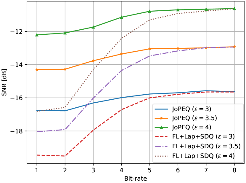
Figure 2: SNR in received models versus compression bit-rate.

We begin by numerically validating that JoPEQ indeed minimizes the excess distortion compared to individual compression and privacy enhancement operating with the same R1-R2. To that aim, we evaluate the average SNR observed at the server before FedAvg, which we compute as the estimated variance of the model weights and divide it by the estimated variance of the distortion, i.e.,

$$\text{SNR}\triangleq\frac{1}{K}\sum_{k=1}^{K}\operatorname*{\text{Var}}(\boldsymbol{h}^{k}_{t})/\operatorname*{\text{Var}}(\boldsymbol{h}^{k}_{t}-\tilde{\boldsymbol{h}}^{k}_{t}).$$

The resulting SNR values of JoPEQ are compared with FL+SDQ+Lap for different privacy budgets $\epsilon\in\{3,3.5,4\}$ in Fig. 2. We observe that JoPEQ yields excess distortion which hardly grows when the bit-rate is decreased, as opposed to separate quantization and Laplace mechanism. The gains of JoPEQ in excess distortion are thus dominant in the low bit regime, where quantization induces notable distortion harnessed by JoPEQ for privacy.

Next, we evaluate how the reduced excess distortion of JoPEQ translates into improved learning.

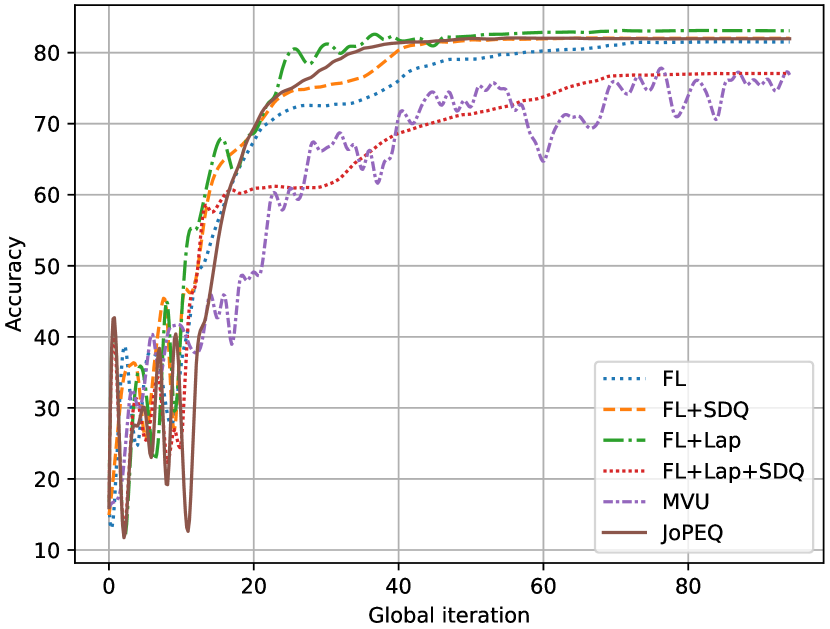
Figure 3: Convergence profile of different scalar FL schemes.

To that aim, we depict in Fig. 3 the validation learning curves for the linear regression model with $R=1$ and $\epsilon=4$. Fig. 3 demonstrates that JoPEQ attains almost equivalent performance compared to the alternatives of FL+SDQ and FL+Lap (which only meet either R1 or R2), while simultaneously satisfying both R1 and R2. We further observe that the disjoint FL+Lap+SDQ as well as the MVU scheme of [34] suffer from excessive distortion as a result of using distinct quantization and privacy mechanism, which deteriorates performance.

TABLE I: Test accuracy results for MNIST

	Linear	MLP	CNN
FL	0.84	0.75	0.79
FL+SDQ	0.84	0.76	0.84
FL+Lap	0.85	0.70	0.77
FL+Lap+SDQ	0.78	0.55	0.75
JoPEQ	0.84	0.70	0.79

In Table I we report the baselines test accuracy of the converged models for different examined architectures, which demonstrates that JoPEQ is beneficial regardless of the model specific design. It is noted that when training deep models, adding a minor level of distortion can improve the converged model, see, e.g., [60, 61]. Hence, FL without privacy or compression does not always achieve the best performance.

IV-A2 CIFAR-10 Dataset

FL is next implemented for the distributed training of natural image classification model using the CIFAR-10 dataset [62]. This set is comprised of $32\times 32$ RGB images divided into $50,000$ training examples and $10,000$ test examples, uniformly distributed among $K=30$ users; each uses local SGD with learning rate $0.1$. The architecture is a CNN composed of three convolutional layers followed by four fully-connected ones, with intermediate ReLU activations, max-pooling and dropout layers, and a softmax output layer.

While MNIST was used to validate scalar encoders ($L=1$), here we consider multivariate approaches as baselines:

FL:

vanilla FL, without privacy or compression constraints.

FL+SDQ$(L=2)$:

SDQ-based compression is now used with lattice dimension $L=2$.

FL+$t$-dist:

denotes the integration of multivariate $t$-distribution mechanism in FL and replaces FL+Lap.

FL+$t$-dist+SDQ$(L=2)$:

the separated application of multivariate $t$-distribution mechanism and SDQ$(L=2)$.

We set the multivariate $t$-distribution parameters to $\boldsymbol{\mu}=\boldsymbol{0}$ and $\mathbf{\Sigma}=s^{2}\boldsymbol{I}_{2}$ where $\boldsymbol{I}_{2}$ denotes the $2\times 2$ identity matrix, and $s^{2},\nu$ are extracted using (11) once $\epsilon$ is given. For SDQ$(L=2)$, we set $\gamma=1.5\times\left(1+s^{2}\nu/(\nu-2)\right)$, numerically assuring low overloading probability.

TABLE II: Test accuracy and SNR results for CIFAR-10

	$R=2,\epsilon=2$		$R=2,\epsilon=3$		$R=1,\epsilon=3$
	Acc.	SNR	Acc.	SNR	Acc.	SNR
FL	0.73	$\infty$	0.73	$\infty$	0.73	$\infty$
FL+SDQ$(L=2)$	0.72	3.53	0.72	3.53	0.72	-5.34
FL+$t$-dist	0.67	-23.51	0.7	-15.55	0.7	-15.55
FL+$t$-dist+SDQ$(L=2)$	0.67	-21.81	0.7	-15.46	0.68	-17.1
JoPEQ	0.68	-21.29	0.71	-14.49	0.7	-14.91

Table II reports the test accuracy and SNR results of the converged baselines for $R\in\{1,2\}$ and $\epsilon\in\{2,3\}$. Comparing the columns of $R=2,\epsilon=2$ and $R=2,\epsilon=3$ demonstrates the privacy budget influence. As expected, higher $\epsilon$ results with less distortion and consequently higher SNR. FL+SDQ$(L=2)$ is invariant to changes in $\epsilon$ values and is the second best, in terms of both accuracy and SNR, after FL without compression and privacy considerations, which suffers from no excess distortion.

The two rightmost columns in Table II highlight the bit-rate effect. Except for FL and FL+$t$-dist, that are bit-rate invariant, all baselines show an improvement for $R=2$ compared to $R=1$. For $R=1,\epsilon=3$ JoPEQ shows the most notable gains compared to the disjoint approach. At the same time, in this extremest bit-rate of $R=1$, the saving in data traffic is the most prominent: in the considered CNN architecture for instance, there are $1.7\cdot 10^{5}$ learnable weights, that are also the amount of bits need to be transmitted in each iteration, instead of $\approx 10^{7}$ bits as in the conventional way where each model parameter is represented with double precision.

IV-B Privacy Leakage Mitigation Evaluation

To empirically validate the ability of JoPEQ to enhance privacy and limit the ability of data leakage attacks, we next assess JoPEQ’s defense performance against model inversion attacks. We consider attacks based on the DLG attack mechanism proposed in [8] applied to invert model updates of neural networks into data samples. In particular, the original DLG generates dummy gradients from dummy inputs, and optimizes the latter to minimize the distance between the former and the real gradients, to yield a successful reconstruction of the training data from the model calculated gradients. This approach was enhanced in [9], which proposed iDLG, that extends DLG to separately reconstruct the label beforehand. In order to examine JoPEQ abilities versus challenging attacks, we use iDLG and take another step further by supplying the attacker with the ground truth label as part of the input.

To that aim, our setup is the one used in [9] and includes the same task (image classification), dataset (CIFAR-10), model architecture (LeNet [63]), and optimizer (L-BFGS [64]). In order to evaluate the results and the quality of the reconstructed images compared to the ground truth, we use structural similarity index measure (SSIM) [65], which is known to reflect image similarity, in addition to mean squared error (MSE). We note that the privacy leakage exploited by DLG can be applied to a general training procedure involving gradients, regardless of whether or not the latter is conducted in a federated manner. Therefore, to focus solely on the ability of JoPEQ to guarantee privacy, we consider a single user. In particular, the raw gradients are either forwarded directly to the iDLG mechanism, or processed beforehand by JoPEQ. Similarly to Subsection IV-A, we also apply iDLG to gradients distorted by SDQ-based compression and by Laplace mechanism.

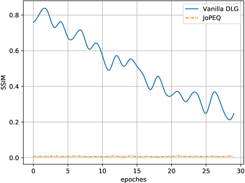
Figure 4: The SSIM score of vanilla DLG and JoPEQ versus epoch number.

We first validate that the ability of JoPEQ to defend from model inversion attacks does not depend on the model training stage, i.e., it can be activated in any given iteration or epoch number. Fig. 4 reports the SSIM score achieved by iDLG applied directly to the gradients (coined vanilla DLG), through $30$ epochs of training, averaged upon the first $70$ CIFAR-10 images; and the results with the incorporation of JoPEQ, for $\epsilon=3$ and $R=8$. Evidently, vanilla DLG struggles more as the training progresses since the gradients tend to be sparser and less informative. However, JoPEQ manages to preserve the privacy from the first iteration, having its associated SSIM metric consistently approaches zero.

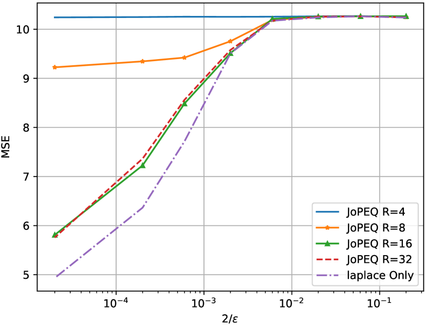
Figure 5: MSE defense score of Laplace mechanism and JoPEQ with different bit-raters, for different privacy budgets.

Next, we evlauate the impact of JoPEQ’s bit-rate budget, given a specific privacy budget $\epsilon$, on its privacy preservation performance under DLG attack, and also compared that to the reference performance of Laplace mechanism. The resulting tradeoff between DLG reconstruction MSE and $2/\epsilon$ are shown in Fig. 5. For fairly loose privacy guarantees, i.e., high $\epsilon$ values, JoPEQ achieves better privacy enhancement compared to Laplace mechanism, i.e., better than that specified by $\epsilon$, as it leads to inferior reconstruction reflected from the high MSE values. For very strong privacy guarantees, JoPEQ with all examined bit-rates as well as Laplace mechanism successfully demolish the input reconstruction, and result with the highest MSE value. Furthermore, an interesting interpretation can be given to the curve describing JoPEQ with $R=4$, which saturates even in the regime of high $\epsilon$ values. According to Theorem III.3, the associated privacy enhancement here is effectively achieved by JoPEQ based solely on its compression-induced distortion, and thus does not involve the introduction of additional PPN.

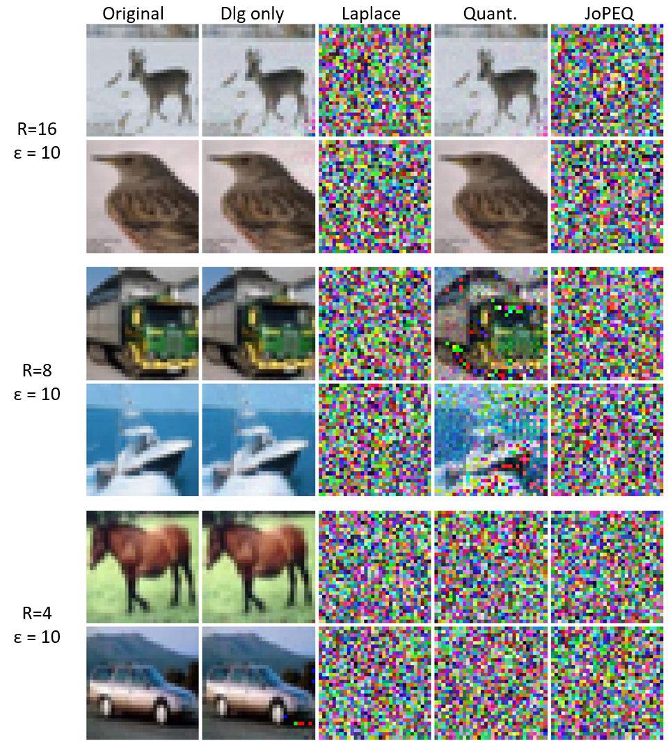
Figure 6: Baselines performances for representative CIFAR-10 examples.

Finally, we visually compare between the baselines performances for several representative images in Fig. 6. As expected, vanilla DLG results in perfect reconstruction and fails under Laplace mechanism integration, for privacy budget of $\epsilon=10$. As for SDQ-based compression, refined quantization holds no privacy defence while a crude one degrades the ability of DLG to reconstruct the image used for training. For quantization with $R=8$, the reconstruction is only damaged up to some extent, but JoPEQ with this same bit-rate can finish up the task, and systematically achieves the same ability to demolish model inversion attacks as the Laplace mechanism. This further assures that JoPEQ, in addition to its being a compression mechanism, is also associated with privacy enhancements.

V Conclusions

We proposed JoPEQ, a unified scheme for jointly compressing and enhancing privacy in FL. JoPEQ utilizes the stochastic nature of SDQ to boost privacy, combining it with a dedicated PPN to yield an exact desired level of distortion satisfying privacy. We proved that JoPEQ can realize different LDP mechanisms, and analyzed its associated distortion and convergence, showing that (under some common assumptions) it achieves similar asymptotic convergence profile as FL without privacy and compression considerations. We applied JoPEQ for the federated training of different models. We numerically demonstrated that it outcomes with less distorted and more reliable models compared with other applications of compression and privacy in FL, while approaching the performance achieved without these constraints, and demolishing common model inversion attacks aim at leaking private date.

-A Proof of Theorem III.1

To prove the theorem, we first note that by (13) and Theorem II.5, it holds that

$$\tilde{\boldsymbol{h}}^{k}_{t,i} =(\zeta_{t}^{k})^{-1}\cdot Q_{\mathcal{L}}^{\rm SDQ}(\zeta_{t}^{k}\boldsymbol{h}^{k}_{t,i}+\boldsymbol{n}^{k}_{i})$$

$$=(\zeta_{t}^{k})^{-1}\cdot(\zeta_{t}^{k}\boldsymbol{h}^{k}_{t,i}+\boldsymbol{n}^{k}_{i}+\boldsymbol{e}^{k}_{i})$$ (-A.1)

$$=\boldsymbol{h}^{k}_{t,i}+(\zeta_{t}^{k})^{-1}(\boldsymbol{n}^{k}_{i}+\boldsymbol{e}^{k}_{i}).$$ (-A.2)

Observing (-A.1), the private scaled updates $\zeta_{t}^{k}\boldsymbol{h}^{k}_{t,i}$ lie in the unit $L$-ball, thus the sensitivity $\left(\Delta\triangleq\max_{x,y\in\mathds{D}}{\|f(x)-f(y)\|}_{2}\right)$ is upper bounded by $\sqrt{2}$. This motivates a specific design of $\boldsymbol{n}^{k}_{i}$ resulting in $\boldsymbol{n}^{k}_{i}+\boldsymbol{e}^{k}_{i}$ representing a multivariate $t$-distribution mechanism (Thm. II.8). Following LDP post-processing property [58], this also implies $\epsilon$-LDP for the non-scaled weights of (-A.2). To do so, we first note the following straightforward lemma, which follows from Thm. II.5:

Lemma -A.1.

$\boldsymbol{e}_{i}^{k}$ and $\boldsymbol{n}_{i}^{k}$ are mutually independent $\forall i,k$.

Next we observe the characteristic function of the overall distortion term. Letting $\boldsymbol{t}={\left[t_{1},\dots,t_{L}\right]}^{T}\in\mathbb{R}^{L}$, by Lemma -A.1 the characteristic function is given by

$$\Phi_{\boldsymbol{n}_{i}^{k}+\boldsymbol{e}_{i}^{k}}(\boldsymbol{t})=\Phi_{\boldsymbol{n}_{i}^{k}}(\boldsymbol{t})\Phi_{\boldsymbol{e}_{i}^{k}}(\boldsymbol{t}),$$ (-A.3)

Recall that $\boldsymbol{e}_{i}^{k}$ distributes uniformly over the basic lattice cell $\mathcal{P}_{0}$, which is also symmetric. Consequently, we can write

$$\Phi_{\boldsymbol{e}_{i}^{k}}(\boldsymbol{t})=\int_{\mathcal{P}_{0}}{\lvert\mathcal{P}_{0}\rvert}^{-1}{\cos\left({\boldsymbol{t}}^{T}{\boldsymbol{e}^{\prime}}_{i}^{k}\right)}d{\boldsymbol{e}^{\prime}}_{i}^{k}.$$ (-A.4)

For (-A.1) to satisfy the multivariate $t$-distribution mechanism, the overall distortion $\boldsymbol{n}^{k}_{i}+\boldsymbol{e}^{k}_{i}$ must be distributed as $\mathbf{t}^{d}_{\nu}(\boldsymbol{\mu},\mathbf{\Sigma})$ which holds (11). Therefore, by [66], for $\boldsymbol{t}\in\mathbb{R}^{d}$ and $\nu>0$ the characteristic function of $\boldsymbol{n}^{k}_{i}+\boldsymbol{e}^{k}_{i}$ satisfies

$$\Phi_{\boldsymbol{n}^{k}_{i}+\boldsymbol{e}^{k}_{i}}(\boldsymbol{t})=\exp(i\boldsymbol{t}^{T}\boldsymbol{\mu})\frac{\|\sqrt{\nu}\boldsymbol{\Sigma}^{1/2}\boldsymbol{t}\|^{\nu/2}}{2^{\nu/2-1}\Gamma(\nu/2)}K_{\nu/2}\left(\|\sqrt{\nu}\boldsymbol{\Sigma}^{1/2}\boldsymbol{t}\|\right).$$ (-A.5)

Finally, combining (-A.3), (-A.4) and (-A.5), we obtain (14).

-B Proof of Theorem III.2

The proof outline is identical to that of Appendix -A with the a single difference in the definition of $\Phi_{\boldsymbol{n}^{k}_{i}+\boldsymbol{e}^{k}_{i}}(\boldsymbol{t})$. For (-A.1) to satisfy Laplace mechanism, the entries of $\boldsymbol{n}^{k}_{i}+\boldsymbol{e}^{k}_{i}\triangleq{\left[n^{k}_{i,1}+e^{k}_{i,1},\dots,n^{k}_{i,L}+e^{k}_{i,L}\right]}^{T}$ must obey an i.i.d. $\operatorname*{\text{Laplace}}\left(0,{2}/{\epsilon}\right)$ distribution. Therefore, the characteristic function of $\boldsymbol{n}^{k}_{i}+\boldsymbol{e}^{k}_{i}$ satisfies

$$\Phi_{\boldsymbol{n}^{k}_{i}+\boldsymbol{e}^{k}_{i}}(\boldsymbol{t}) =\prod_{l=1}^{L}\Phi_{n^{k}_{i,l}+e^{k}_{i,l}}\left(t_{l}\right)=\prod_{l=1}^{L}\frac{1}{1+{\left(2t_{l}/\epsilon\right)}^{2}},$$

proving the theorem.

-C Proof of Theorem III.3

Assuming JoPEQ operates with a lattice quantizer of dimension $L=1$ and holds the Laplace mechanism, the $l$th entry of $\boldsymbol{n}^{k}_{i}+\boldsymbol{e}^{k}_{i}$ satisfies

$$\operatorname*{\text{Var}}[n^{k}_{i,l}+e^{k}_{i,l}]=\operatorname*{\text{Var}}\left[\operatorname*{\text{Laplace}}\left(\mu=0,b=2/\epsilon\right)\right]=2b^{2}.$$

On the other hand, using Lemma -A.1,

$$\operatorname*{\text{Var}}[n^{k}_{i,l}+e^{k}_{i,l}]=\operatorname*{\text{Var}}[n^{k}_{i,l}]+\operatorname*{\text{Var}}[e^{k}_{i,l}].$$

That is, for infinitely small variance PPN, JoPEQ with dynamic rage $\gamma$ and bit-rate $R$ holds $\epsilon$-LDP as long as

$$2b^{2}\leq \operatorname*{\text{Var}}[e^{k}_{i,l}]\overset{(a)}{=}\operatorname*{\text{Var}}\left[\mathcal{U}\left(\frac{-\Delta_{\rm Q}}{2},\frac{\Delta_{\rm Q}}{2}\right)\right]={\Delta_{\rm Q}^{2}}/{12},$$

where (a) follows from Theorem II.5 using $L=1$, and $\mathcal{U}(\cdot)$ denotes the continuous uniform distribution. Substituting the fact that $\Delta_{\rm Q}=2\gamma/2^{R}$ and $b=2/\epsilon$ we obtain

$$2(2/\epsilon)^{2}\leq {(2\gamma/2^{R})^{2}}/{12},$$ (-C.1)

which is equivalent to $\sqrt{24}\leq\varphi\epsilon/2^{R}$, concluding the proof.

-D Proof of Theorem III.4

Our proof follows a similar outline to that used in [21], with the introduction of additional arguments for handling privacy constraints, in addition to those of quantization. The unique characteristics of JoPEQ’s error, which follow from the SDQ strategy presented in Section III, allow us to rigorously incorporate its contribution into the overall proof flow.

In order to bound $\mathds{E}\left\{\|\tilde{\boldsymbol{w}}_{t+\tau}-\boldsymbol{w}_{t+\tau}\|^{2}\right\}$ let us first express the weights distortion term $\tilde{\boldsymbol{w}}_{t+\tau}-\boldsymbol{w}_{t+\tau}$, where $\tilde{\boldsymbol{w}}_{t+\tau},\boldsymbol{w}_{t+\tau}$ are defined in (17), (2) respectively. We denote by $\{\boldsymbol{v}_{i}\}_{i=1}^{M}$ the decomposition of a vector $\boldsymbol{v}$ into $M$ distinct $L\times 1$ sub-vectors. It is easy to verify that for $\zeta_{t}^{k}=\left(\frac{3}{\sqrt{M}}\|\boldsymbol{h}^{k}_{t}\|\right)^{-1}$ we have

$$\tilde{\boldsymbol{w}}_{t+\tau,i}=\boldsymbol{w}_{t+\tau,i}+\sum_{k=1}^{K}\alpha_{k}\underbrace{\left(\tilde{\boldsymbol{h}}^{k}_{t+\tau,i}-\boldsymbol{h}^{k}_{t+\tau,i}\right)}_{=3\|\boldsymbol{h}^{k}_{t+\tau}\|(\boldsymbol{n}^{k}_{i}+\boldsymbol{e}^{k}_{i})/\sqrt{M}}.$$

Consequently,

$$\mathds{E}\left\{\|\tilde{\boldsymbol{w}}_{t+\tau}-\boldsymbol{w}_{t+\tau}\|^{2}\right\}\overset{(a)}{=}$$

$$\mathds{E}\left\{\mathds{E}\left\{\left.\left\|\sum_{i=1}^{M}\sum_{k=1}^{K}\alpha_{k}\frac{3}{\sqrt{M}}\|\boldsymbol{h}^{k}_{t+\tau}\|(\boldsymbol{n}^{k}_{i}+\boldsymbol{e}^{k}_{i})\right\|^{2}\right|\boldsymbol{h}^{k}_{t+\tau}\right\}\right\}\overset{(b)}{=}$$

$$\mathds{E}\left\{9\sum_{k=1}^{K}\alpha_{k}^{2}\|\boldsymbol{h}^{k}_{t+\tau}\|^{2}\mathds{E}\left\{\left.\left\|(\boldsymbol{n}^{k}_{i}+\boldsymbol{e}^{k}_{i})\right\|^{2}\right|\boldsymbol{h}^{k}_{t+\tau}\right\}\right\}=$$

$$\mathds{E}\left\{9\sigma^{2}\sum_{k=1}^{K}\alpha_{k}^{2}\|\boldsymbol{h}^{k}_{t+\tau}\|^{2}\right\},$$ (-D.1)

where (a) follows from the law of total expectation. According to either Theorem II.8 or II.7, $\{\boldsymbol{n}^{k}_{i}+\boldsymbol{e}^{k}_{i}\}$ are i.i.d. with $\mathds{E}\left\{\left\|(\boldsymbol{n}^{k}_{i}+\boldsymbol{e}^{k}_{i})\right\|^{2}\right\}=\sigma^{2}$ . Therefore, (b) holds by the triangle equality. Next, if we iterate recursively over (3), the model update $\boldsymbol{h}^{k}_{t+\tau}=\boldsymbol{w}^{k}_{t+\tau}-\boldsymbol{w}_{t}$ can be written as the sum of the stochastic gradients $\boldsymbol{h}^{k}_{t+\tau}=-\sum_{t^{\prime}=t}^{t+\tau-1}\eta_{t^{\prime}}\nabla F_{k}^{i^{k}_{t^{\prime}}}\left(\boldsymbol{w}^{k}_{t^{\prime}}\right)$; where stochasticity stems from the uniformly distributed random indexes $i^{k}_{t^{\prime}}$. To utilize this, we first apply the law of total expectation to (-D) to yield

$$\mathds{E}\left\{\|\tilde{\boldsymbol{w}}_{t+\tau}-\boldsymbol{w}_{t+\tau}\|^{2}\right\}=$$

$$\mathds{E}\left\{9\sigma^{2}\sum_{k=1}^{K}\alpha_{k}^{2}\mathds{E}\left\{\left.\left\|\sum_{t^{\prime}=t}^{t+\tau-1}\eta_{t^{\prime}}\nabla F_{k}^{i^{k}_{t^{\prime}}}\left(\boldsymbol{w}^{k}_{t^{\prime}}\right)\right\|^{2}\right|\left\{\boldsymbol{w}^{k}_{t^{\prime}}\right\}\right\}\right\}\overset{(a)}{\leq}$$

$$\mathds{E}\left\{9\sigma^{2}\sum_{k=1}^{K}\alpha_{k}^{2}\tau\sum_{t^{\prime}=t}^{t+\tau-1}\eta_{t^{\prime}}^{2}\mathds{E}\left\{\left.\|\nabla F_{k}^{i^{k}_{t^{\prime}}}\left(\boldsymbol{w}^{k}_{t^{\prime}}\right)\|^{2}\right|\left\{\boldsymbol{w}^{k}_{t^{\prime}}\right\}\right\}\right\}\overset{(b)}{\leq}$$

$$9\tau\sigma^{2}\left(\sum_{t^{\prime}=t}^{t+\tau-1}\eta_{t^{\prime}}^{2}\right)\sum_{k=1}^{K}\alpha_{k}^{2}\xi^{2}_{k},$$ (-D.2)

where (a) follows from Jensen’s inequality $\|\sum_{t^{\prime}=t}^{t+\tau-1}\boldsymbol{v}_{t}\|^{2}\leq\tau\sum_{t^{\prime}=t}^{t+\tau-1}\|\boldsymbol{v}_{t}\|^{2}$, viewing the $\ell_{2}$-norm as a real convex function; and (b) holds since $\mathds{E}\left\{\|\nabla F_{k}^{i^{k}_{t^{\prime}}}\left(\boldsymbol{w}^{k}_{t^{\prime}}\right)\|^{2}\right\}\leq\xi^{2}_{k}$ by AS2. Finally, (-D) proves the theorem.

-E Proof of Theorem III.5

In the sequel we follow [21] and first derive a recursive bound on the weights error, from which we conclude the FL convergence bound.

-E1 Recursive Bound on Weights Error

Recall that every $\tau$ local SGD iterations, the $k$th user performs a transmission, that once done with JoPEQ integration, its effect can be modeled as additional noise via $\tilde{\boldsymbol{h}}^{k}_{t}=\boldsymbol{h}^{k}_{t}+\text{err}_{t}^{k}$. Thus, $\text{err}_{t}^{k}=\boldsymbol{0}$ when $t$ is an integer multiple of $\tau$ and otherwise, by Appendix -A, each $L\times 1$ sub-vector of $\text{err}_{t}^{k}$ scaled by $\zeta_{t}^{k}$ obeys the multivariate $t$-distribution $\mathbf{t}^{d}_{\nu}(\boldsymbol{\mu},\mathbf{\Sigma})$ which holds (11). The overall procedure can be compactly written as

$$\boldsymbol{w}^{k}_{t+1}=$$

$$\begin{cases*}\boldsymbol{w}^{k}_{t}-\eta_{t}\nabla F_{k}^{i^{k}_{t}}\left(\boldsymbol{w}^{k}_{t}\right)+\underbrace{\text{err}_{t}^{k}}_{=0}\quad\text{ if }t+1\neq n\cdot\tau,\ n\in\mathbb{N},\\ \sum_{k^{\prime}=1}^{K}\alpha_{k^{\prime}}\left(\boldsymbol{w}^{k^{\prime}}_{t}-\eta_{t}\nabla F_{k^{\prime}}^{i^{k^{\prime}}_{t}}\left(\boldsymbol{w}^{k^{\prime}}_{t}\right)+\text{err}_{t}^{k^{\prime}}\right)\quad\text{ else}.\end{cases*}$$

As in [21], we next define $\boldsymbol{v}_{t}\triangleq\sum_{k=1}^{K}\alpha_{k}\boldsymbol{w}^{k}_{t}$, and the averaged noisy stochastic as well as the full gradients

$$\tilde{\boldsymbol{g}}_{t} \triangleq\sum_{k=1}^{K}\alpha_{k}\left(\nabla F_{k}^{i^{k}_{t}}\left(\boldsymbol{w}^{k}_{t}\right)-\frac{1}{\eta_{t}}\text{err}_{t}^{k}\right),$$ (-E.1)

$$\boldsymbol{g}_{t} \triangleq\sum_{k=1}^{K}\alpha_{k}\nabla F_{k}\left(\boldsymbol{w}^{k}_{t}\right),$$ (-E.2)

respectively. Note that for the specific choice of $\mathbf{t}^{d}_{\nu}(\boldsymbol{0},\mathbf{\Sigma})$ JoPEQ’s error is zero-mean, and it further holds that $\mathds{E}\{\tilde{\boldsymbol{g}}_{t}\}=\boldsymbol{g}_{t}$ and $\boldsymbol{v}_{t+1}=\boldsymbol{v}_{t}-\eta_{t}\tilde{\boldsymbol{g}}_{t}$.

The resulting model is thus equivalent to that used in [21, App. C], and therefore, by assumptions 3-4 it follows that if $\eta_{t}\leq\frac{1}{4\rho_{s}}$ then

$$\mathds{E}\left\{\left\|\boldsymbol{v}_{t+1}-\boldsymbol{w}^{\rm opt}\right\|^{2}\right\}\leq(1-\eta_{t}\rho_{c})\mathds{E}\left\{\left\|\boldsymbol{v}_{t}-\boldsymbol{w}^{\rm opt}\right\|^{2}\right\}\\ +6\rho_{s}\eta^{2}_{t}\psi+\eta^{2}_{t}\mathds{E}\left\{\left\|\tilde{\boldsymbol{g}}_{t}-\boldsymbol{g}_{t}\right\|^{2}\right\}\\ +2\mathds{E}\left\{\sum_{k=1}^{K}\alpha_{k}\left\|\boldsymbol{v}_{t}-\boldsymbol{w}^{k}_{t}\right\|^{2}\right\},$$ (-E.3)

where $\boldsymbol{w}^{\rm opt},\ \psi$ are defined in (1), (19) respectively. We further bound the summands in (-E.3), using Lemmas C.1 and C.2 in [21, App. C]

$$\eta^{2}_{t}\mathds{E}\left\{\left\|\tilde{\boldsymbol{g}}_{t}-\boldsymbol{g}_{t}\right\|^{2}\right\}\leq\left(1+36\tau^{2}\sigma^{2}\right)\eta_{t}^{2}\sum_{k=1}^{K}\alpha_{k}^{2}\xi^{2}_{k},$$ (-E.4)

$$\mathds{E}\left\{\sum_{k=1}^{K}\alpha_{k}\left\|\boldsymbol{v}_{t}-\boldsymbol{w}^{k}_{t}\right\|^{2}\right\}\leq 4(\tau-1)^{2}\eta_{t}^{2}\sum_{k=1}^{K}\alpha_{k}\xi^{2}_{k}.$$ (-E.5)

Next, we define $\delta_{t}\triangleq\mathds{E}\left\{\left\|\boldsymbol{v}_{t}-\boldsymbol{w}^{\rm opt}\right\|^{2}\right\}$. When $t=n\cdot\tau,\ n\in\mathbb{N}$, the term $\delta_{t}$ represents the $\ell_{2}$-norm of the error in the weights of the global model. Integrating (-E.4) and (-E.5) into (-E.3), we obtain the following recursive relationship on the weights error:

$$\delta_{t+1} \leq(1-\eta_{t}\rho_{c})\delta_{t}+\eta^{2}_{t}b,\text{ where }$$ (-E.6)

$$b \triangleq\left(1+36\tau^{2}\sigma^{2}\right)\sum_{k=1}^{K}\alpha^{2}_{k}\xi^{2}_{k}+6\rho_{s}\psi+8(\tau-1)^{2}\sum_{k=1}^{K}\alpha_{k}\xi^{2}_{k}.$$

The relationship in (-E.6) is used in the sequel to prove the FL convergence bound stated in Theorem III.5.

-E2 FL Convergence Bound

We set the step-size $\eta_{t}$ to take the form $\eta_{t}=\frac{\beta}{t+\varphi}$ for some $\beta>0$ and $\varphi\geq\max(4\rho_{s}\beta,\tau)$, for which $\eta_{t}\leq\frac{1}{4\rho_{s}}$ and $\eta_{t}\leq 2\eta_{t+\tau}$, implying that (-E.3), (-E.4) and (-E.5) hold. Under such settings, in [21, App. C] is it proved by induction that for $\lambda\geq\max\left(\frac{1+\beta^{2}b}{\beta\rho_{c}},\varphi\delta_{0}\right)$, it holds that $\delta_{t}\leq\frac{\lambda}{t+\varphi}$ for all integer $t\geq 0$. Finally, the smoothness of the objective 3 implies that

$$\mathds{E}\{F(\boldsymbol{w}_{t})-F(\boldsymbol{w}^{\rm opt})\}\leq\frac{\rho_{s}}{2}\delta_{t}\leq\frac{\rho_{2}\lambda}{2(t+\varphi)}.$$ (-E.7)

Setting $\beta=\frac{\tau}{\rho_{c}}$ results in $\varphi\geq\tau\max(1,4\rho_{s}/\rho_{c})$ and $\lambda\geq\max(\frac{\rho^{2}_{c}+\tau^{2}b}{\tau\rho_{c}},\varphi\delta_{0})$, once substituted into (-E.7), proves (20).

References

- [1] N. Lang and N. Shlezinger, “Joint privacy enhancement and quantization in federated learning,” in IEEE International Symposium on Information Theory (ISIT), 2022, pp. 2040–2045.
- [2] B. McMahan, E. Moore, D. Ramage, S. Hampson, and B. A. y Arcas, “Communication-efficient learning of deep networks from decentralized data,” in Artificial intelligence and statistics. PMLR, 2017, pp. 1273–1282.
- [3] P. Kairouz, H. B. McMahan, B. Avent, A. Bellet, M. Bennis, A. N. Bhagoji, K. Bonawitz, Z. Charles, G. Cormode, R. Cummings et al., “Advances and open problems in federated learning,” Foundations and Trends® in Machine Learning, vol. 14, no. 1–2, pp. 1–210, 2021.
- [4] T. Li, A. K. Sahu, A. Talwalkar, and V. Smith, “Federated learning: Challenges, methods, and future directions,” IEEE Signal Process. Mag., vol. 37, no. 3, pp. 50–60, 2020.
- [5] T. Gafni, N. Shlezinger, K. Cohen, Y. C. Eldar, and H. V. Poor, “Federated learning: A signal processing perspective,” IEEE Signal Process. Mag., vol. 39, no. 3, pp. 14–41, 2022.
- [6] J. Chen and X. Ran, “Deep learning with edge computing: A review.” Proc. IEEE, vol. 107, no. 8, pp. 1655–1674, 2019.
- [7] M. Chen, N. Shlezinger, H. V. Poor, Y. C. Eldar, and S. Cui, “Communication-efficient federated learning,” Proceedings of the National Academy of Sciences, vol. 118, no. 17, 2021.
- [8] L. Zhu and S. Han, “Deep leakage from gradients,” in Federated learning. Springer, 2020, pp. 17–31.
- [9] B. Zhao, K. R. Mopuri, and H. Bilen, “iDLG: Improved deep leakage from gradients,” arXiv preprint arXiv:2001.02610, 2020.
- [10] Y. Huang, S. Gupta, Z. Song, K. Li, and S. Arora, “Evaluating gradient inversion attacks and defenses in federated learning,” Advances in Neural Information Processing Systems, vol. 34, 2021.
- [11] H. Yin, A. Mallya, A. Vahdat, J. M. Alvarez, J. Kautz, and P. Molchanov, “See through gradients: Image batch recovery via gradinversion,” in Proceedings of the IEEE/CVF Conference on Computer Vision and Pattern Recognition, 2021, pp. 16 337–16 346.
- [12] Y. Lin, S. Han, H. Mao, Y. Wang, and W. J. Dally, “Deep gradient compression: Reducing the communication bandwidth for distributed training,” arXiv preprint arXiv:1712.01887, 2017.
- [13] D. Alistarh, T. Hoefler, M. Johansson, N. Konstantinov, S. Khirirat, and C. Renggli, “The convergence of sparsified gradient methods,” Advances in Neural Information Processing Systems, vol. 31, 2018.
- [14] P. Han, S. Wang, and K. K. Leung, “Adaptive gradient sparsification for efficient federated learning: An online learning approach,” in IEEE International Conference on Distributed Computing Systems (ICDCS), 2020, pp. 300–310.
- [15] J. Konečnỳ, H. B. McMahan, F. X. Yu, P. Richtárik, A. T. Suresh, and D. Bacon, “Federated learning: Strategies for improving communication efficiency,” arXiv preprint arXiv:1610.05492, 2016.
- [16] C. Hardy, E. Le Merrer, and B. Sericola, “Distributed deep learning on edge-devices in the parameter server model,” in Workshop on Decentralized Machine Learning, Optimization and Privacy, 2017, p. 1.
- [17] A. F. Aji and K. Heafield, “Sparse communication for distributed gradient descent,” arXiv preprint arXiv:1704.05021, 2017.
- [18] D. Alistarh, D. Grubic, J. Li, R. Tomioka, and M. Vojnovic, “QSGD: Communication-efficient SGD via gradient quantization and encoding,” Advances in Neural Information Processing Systems, vol. 30, pp. 1709–1720, 2017.
- [19] A. Reisizadeh, A. Mokhtari, H. Hassani, A. Jadbabaie, and R. Pedarsani, “Fedpaq: A communication-efficient federated learning method with periodic averaging and quantization,” in International Conference on Artificial Intelligence and Statistics. PMLR, 2020, pp. 2021–2031.
- [20] J. Bernstein, Y.-X. Wang, K. Azizzadenesheli, and A. Anandkumar, “signSGD: Compressed optimisation for non-convex problems,” in International Conference on Machine Learning. PMLR, 2018, pp. 560–569.
- [21] N. Shlezinger, M. Chen, Y. C. Eldar, H. V. Poor, and S. Cui, “UVeQFed: Universal vector quantization for federated learning,” IEEE Trans. Signal Process., vol. 69, pp. 500–514, 2020.
- [22] S. P. Karimireddy, Q. Rebjock, S. Stich, and M. Jaggi, “Error feedback fixes signsgd and other gradient compression schemes,” in International Conference on Machine Learning. PMLR, 2019, pp. 3252–3261.
- [23] S. Horvath, C.-Y. Ho, L. Horvath, A. N. Sahu, M. Canini, and P. Richtárik, “Natural compression for distributed deep learning,” arXiv preprint arXiv:1905.10988, 2019.
- [24] M. Kim, O. Günlü, and R. F. Schaefer, “Federated learning with local differential privacy: Trade-offs between privacy, utility, and communication,” in IEEE International Conference on Acoustics, Speech and Signal Processing (ICASSP), 2021, pp. 2650–2654.
- [25] K. Wei, J. Li, M. Ding, C. Ma, H. H. Yang, F. Farokhi, S. Jin, T. Q. Quek, and H. V. Poor, “Federated learning with differential privacy: Algorithms and performance analysis,” IEEE Trans. Inf. Forensics Security, vol. 15, pp. 3454–3469, 2020.
- [26] L. Sun, J. Qian, X. Chen, and P. S. Yu, “LDP-FL: Practical private aggregation in federated learning with local differential privacy,” arXiv preprint arXiv:2007.15789, 2020.
- [27] R. Liu, Y. Cao, M. Yoshikawa, and H. Chen, “Fedsel: Federated SGD under local differential privacy with top-k dimension selection,” in International Conference on Database Systems for Advanced Applications. Springer, 2020, pp. 485–501.
- [28] M. Seif, R. Tandon, and M. Li, “Wireless federated learning with local differential privacy,” in IEEE International Symposium on Information Theory (ISIT), 2020, pp. 2604–2609.
- [29] D. Liu and O. Simeone, “Privacy for free: Wireless federated learning via uncoded transmission with adaptive power control,” IEEE J. Sel. Areas Commun., vol. 39, no. 1, pp. 170–185, 2020.
- [30] T. Liu, B. Di, B. Wang, and L. Song, “Loss-privacy tradeoff in federated edge learning,” IEEE J. Sel. Topics Signal Process., vol. 16, no. 3, pp. 546–558, 2022.
- [31] L. Lyu, “DP-SIGNSGD: When efficiency meets privacy and robustness,” in IEEE International Conference on Acoustics, Speech and Signal Processing (ICASSP), 2021, pp. 3070–3074.
- [32] Y. Zhang, D. Liu, and O. Simeone, “Leveraging channel noise for sampling and privacy via quantized federated langevin monte carlo,” in IEEE International Workshop on Signal Processing Advances in Wireless Communication (SPAWC), 2022.
- [33] S. Amiri, A. Belloum, S. Klous, and L. Gommans, “Compressive differentially private federated learning through universal vector quantization,” in AAAI Workshop on Privacy-Preserving Artificial Intelligence, 2021.
- [34] K. Chaudhuri, C. Guo, and M. Rabbat, “Privacy-aware compression for federated data analysis,” in The 38th Conference on Uncertainty in Artificial Intelligence, 2022.
- [35] R. Zamir and M. Feder, “On universal quantization by randomized uniform/lattice quantizers,” IEEE Trans. Inf. Theory, vol. 38, no. 2, pp. 428–436, 1992.
- [36] ——, “On lattice quantization noise,” IEEE Trans. Inf. Theory, vol. 42, no. 4, pp. 1152–1159, 1996.
- [37] M. Reimherr and J. Awan, “Elliptical perturbations for differential privacy,” in Advances in Neural Information Processing Systems, vol. 32, 2019.
- [38] S. U. Stich, “Local SGD converges fast and communicates little,” in The International Conference on Learning Representations, 2019.
- [39] R. M. Gray and D. L. Neuhoff, “Quantization,” IEEE Trans. Inf. Theory, vol. 44, no. 6, pp. 2325–2383, 1998.
- [40] Y. Polyanskiy and Y. Wu, “Lecture notes on information theory,” Lecture Notes for 6.441 (MIT), ECE563 (University of Illinois Urbana-Champaign), and STAT 664 (Yale), 2012-2017.
- [41] S. P. Lipshitz, R. A. Wannamaker, and J. Vanderkooy, “Quantization and dither: A theoretical survey,” Journal of the audio engineering society, vol. 40, no. 5, pp. 355–375, 1992.
- [42] R. M. Gray and T. G. Stockham, “Dithered quantizers,” IEEE Trans. Inf. Theory, vol. 39, no. 3, pp. 805–812, 1993.
- [43] X. Yang, T. Wang, X. Ren, and W. Yu, “Survey on improving data utility in differentially private sequential data publishing,” IEEE Trans. Big Data, 2017.
- [44] J. M. Abowd, “The US census bureau adopts differential privacy,” in Proceedings of the 24th ACM SIGKDD International Conference on Knowledge Discovery & Data Mining, 2018, pp. 2867–2867.
- [45] S. P. Kasiviswanathan, H. K. Lee, K. Nissim, S. Raskhodnikova, and A. Smith, “What can we learn privately?” SIAM Journal on Computing, vol. 40, no. 3, pp. 793–826, 2011.
- [46] Y. Wang, Y. Tong, and D. Shi, “Federated latent dirichlet allocation: A local differential privacy based framework,” in Proceedings of the AAAI Conference on Artificial Intelligence, vol. 34, no. 04, 2020, pp. 6283–6290.
- [47] T. Wang, X. Zhang, J. Feng, and X. Yang, “A comprehensive survey on local differential privacy toward data statistics and analysis,” Sensors, vol. 20, no. 24, p. 7030, 2020.
- [48] C. Dwork, F. McSherry, K. Nissim, and A. Smith, “Calibrating noise to sensitivity in private data analysis,” Journal of Privacy and Confidentiality, vol. 7, no. 3, pp. 17–51, 2016.
- [49] K. Chaudhuri, C. Monteleoni, and A. D. Sarwate, “Differentially private empirical risk minimization.” Journal of Machine Learning Research, vol. 12, no. 3, 2011.
- [50] D. Kifer and A. Machanavajjhala, “Pufferfish: A framework for mathematical privacy definitions,” ACM Transactions on Database Systems (TODS), vol. 39, no. 1, pp. 1–36, 2014.
- [51] J. Awan and A. Slavković, “Structure and sensitivity in differential privacy: Comparing k-norm mechanisms,” Journal of the American Statistical Association, vol. 116, no. 534, pp. 935–954, 2021.
- [52] Y. Zhao, J. Zhao, M. Yang, T. Wang, N. Wang, L. Lyu, D. Niyato, and K.-Y. Lam, “Local differential privacy-based federated learning for internet of things,” IEEE Internet Things J., vol. 8, no. 11, pp. 8836–8853, 2020.
- [53] J. H. Conway and N. J. A. Sloane, Sphere Packings, Lattices and Groups. Springer Science & Business Media, 2013, vol. 290.
- [54] K. Ferentios, “On Tcebycheff’s type inequalities,” Trabajos de Estadistica y de Investigacion Operativa, vol. 33, no. 1, p. 125, 1982.
- [55] N. Shlezinger, S. Rini, and Y. C. Eldar, “The communication-aware clustered federated learning problem,” in IEEE International Symposium on Information Theory (ISIT), 2020, pp. 2610–2615.
- [56] X. Li, K. Huang, W. Yang, S. Wang, and Z. Zhang, “On the convergence of fedavg on non-iid data,” arXiv preprint arXiv:1907.02189, 2019.
- [57] Y. Zhang, M. J. Wainwright, and J. C. Duchi, “Communication-efficient algorithms for statistical optimization,” Advances in neural information processing systems, vol. 25, 2012.
- [58] X. Xiong, S. Liu, D. Li, Z. Cai, and X. Niu, “A comprehensive survey on local differential privacy,” Security and Communication Networks, vol. 2020, 2020.
- [59] L. Deng, “The MNIST database of handwritten digit images for machine learning research,” IEEE Signal Process. Mag., vol. 29, no. 6, pp. 141–142, 2012.
- [60] G. An, “The effects of adding noise during backpropagation training on a generalization performance,” Neural computation, vol. 8, no. 3, pp. 643–674, 1996.
- [61] T. Sery, N. Shlezinger, K. Cohen, and Y. C. Eldar, “Over-the-air federated learning from heterogeneous data,” IEEE Trans. Signal Process., vol. 69, pp. 3796–3811, 2021.
- [62] A. Krizhevsky, V. Nair, and G. Hinton, “Cifar-10 (canadian institute for advanced research).” [Online]. Available: http://www.cs.toronto.edu/~kriz/cifar.html
- [63] Y. LeCun, B. Boser, J. S. Denker, D. Henderson, R. E. Howard, W. Hubbard, and L. D. Jackel, “Backpropagation applied to handwritten zip code recognition,” Neural computation, vol. 1, no. 4, pp. 541–551, 1989.
- [64] D. C. Liu and J. Nocedal, “On the limited memory bfgs method for large scale optimization,” Mathematical programming, vol. 45, no. 1, pp. 503–528, 1989.
- [65] Z. Wang, A. C. Bovik, H. R. Sheikh, and E. P. Simoncelli, “Image quality assessment: from error visibility to structural similarity,” IEEE Trans. Image Process., vol. 13, no. 4, pp. 600–612, 2004.
- [66] D.-K. Song, H.-J. Park, and H.-M. Kim, “A note on the characteristic function of multivariate t distribution,” Communications for Statistical Applications and Methods, vol. 21, no. 1, pp. 81–91, 2014.